


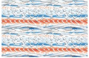


1. Introduction
The unsteady flows are ubiquitous in nature and their transitions from laminar to turbulent are fundamental issues of concern in hydrodynamic stability theory. Other than being the prototype problem in the dynamics of sediment transport along coastal areas, the characteristics of boundary layers induced by oscillatory flow, pulsatile flow and solitary waves have been found to be essential for other fields such as biological processes (e.g. Xu et al. Reference Xu, Varshney, Ma, Song, Riedl, Avila and Ho2020; Xu, Song & Avila Reference Xu, Song and Avila2021). Compared with its steady counterpart, the instantaneous shifting pressure gradient and velocity profile substantially alter the stability characteristics and further complicate the relevant transition scenarios to turbulence. Much has been contributed to the understanding of the instabilities of the most canonical unsteady boundary layer generated by oscillatory flow or equivalently by sinusoidally oscillating plate, also known as a Stokes boundary layer, from the perspectives of coherent structures (Sarpkaya Reference Sarpkaya1993; Özdemir, Hsu & Balachandar Reference Özdemir, Hsu and Balachandar2014; Xiong et al. Reference Xiong, Qi, Gao, Xu, Ren and Cheng2020), linear stability analyses (Kerczek & Davis Reference Kerczek and Davis1974; Hall Reference Hall1978; Blennerhassett & Bassom Reference Blennerhassett and Bassom2006; Thomas et al. Reference Thomas, Davies, Bassom and Blennerhassett2014) and statistical features (Hino et al. Reference Hino, Kashiwayanagi, Nakayama and Hara1983; Sleath Reference Sleath1987; Jensen, Sumer & Fredsoe Reference Jensen, Sumer and Fredsoe1989). The theoretical solution of the Stokes boundary layer explicitly provides the time-dependent distribution of streamwise velocity along the wall-normal direction (Stokes Reference Stokes1851). The velocity profile is merely dependent on one dimensionless parameter, i.e. the Reynolds number defined by  $Re_\delta = U_{0m}^*\delta ^*/\nu ^*$, where
 $U_{0m}^*$ is the velocity amplitude of the oscillatory free-stream flow and
 $\nu ^*$ is the kinematic viscosity of the fluid. In addition, the boundary-layer thickness
 $\delta ^*$ is evaluated by
 $\delta ^*=\sqrt {2\nu ^*/\varOmega ^*}$ with
 $\varOmega ^*$ being the oscillatory frequency. However, the bypass nature characterised by the onset of streaky structures in numerical and experimental observations at
 $Re_\delta >500$ (Costamagna, Vittori & Blondeaux Reference Costamagna, Vittori and Blondeaux2003; Carstensen, Sumer & Fredsøe Reference Carstensen, Sumer and Fredsøe2010) has not been well elaborated by the theoretical studies. The secondary instabilities arising from the transient growth and nonlinear saturation of the primary instability are possibly responsible for the large deviation of the critical Reynolds numbers that were obtained from numerical or experimental studies and linear modal stability analyses, e.g.
 $Re_{\delta,cr}=\infty$ (instantaneous instability theory, Hall Reference Hall1978, Reference Hall2003) and
 $Re_{\delta,cr}=1416$ (Floquet instability theory, Blennerhassett & Bassom Reference Blennerhassett and Bassom2002, Reference Blennerhassett and Bassom2006). An ultimate objective of this study is to provide a universal understanding on the role of the Orr mechanism and the lift-up effect corresponding to the formation of different two-dimensional (2-D) and three-dimensional (3-D) coherent structures. Their evolution, competition, interaction and the final breakdown to turbulence under the unsteady pressure gradient are our primary interests.
It is well known that Tollmien–Schlichting (T–S) waves originally arise as the primary 2-D instabilities in steady shear flows. T–S waves correspond to exponentially growing eigenmodes of the Orr–Sommerfeld and Squire (OSS) equations, and readers may refer to Schmid & Henningson (Reference Schmid and Henningson2001) for details. As indicated in the schematic diagram of figure 1, the modal growth of T–S waves, after reaching the critical magnitude, leads to the emergence of secondary 3-D instabilities in the form of  $\varLambda$-/hairpin vortices with aligned or staggered spatial patterns corresponding to the Klebanoff (K) mode and Herbert (H) mode, respectively (Herbert Reference Herbert1988). However, the transition scenarios by modal growth of perturbations have rarely been observed in the Stokes boundary layer. It is believed that the instantaneous inflectional mean profile resulting from reverse flow leads to the transient growth of 2-D waves and to the onset of spanwise vortices (figure 1). These quasi-2-D coherent structures, referred to as vortex tubes by Carstensen et al. (Reference Carstensen, Sumer and Fredsøe2010) and Sumer et al. (Reference Sumer, Jensen, Sorensen, Fredsøe, Liu and Carstensen2010), are observed in oscillatory and solitary wave boundary layers. In the 2-D numerical study of Scandura (Reference Scandura2013), it was demonstrated that for both unsteady boundary layers these vortex tubes consist of an array of counter-rotating vortex pairs with almost identical configurations and similar spatial-temporal characteristics. The latest experimental effort by Nayak & Das (Reference Nayak and Das2021), employing particle image velocimetry measurement, identified similar coherent vortices developed in a transient pipe flow with trapezoidal velocity variation. The above results suggest that the non-modal growth mechanism may apply for more generalised unsteady boundary-layer flows with the inflectional point located in the high-shear region. The optimal initial perturbation for the maximum transient amplification of an oscillatory boundary layer has been determined by Biau (Reference Biau2016) through non-modal stability analyses. Unlike the instantaneous or Floquet stability analysis for the steady or periodic time-dependent base flow, the non-modal stability analysis (alternatively named transient stability analysis) is carried out on aperiodic base flow with an arbitrary period of time. The perturbation amplification by non-modal growth is reminiscent of the classic Orr mechanism observed in steady shear flow with a homogeneous strain rate, which signifies the absorption of energy from the mean shear by vortex tilting. Whereas the time-dependent and heterogeneous strain rate along the velocity profile of an oscillatory wave boundary layer renders considerable modulation of the classic Orr mechanism, to manifest such a difference, the terminology ‘Orr-like mechanism’ is adopted and the corresponding physics will be discussed in § 3.1.
Schematic diagram of transition scenarios of steady or unsteady parallel boundary-layer flows.

As sketched in figure 1, the secondary instabilities of the vortex tube, which generally occur with increasing  $Re_\delta$ and disturbance level, are classified into two categories according to various experimental (Carstensen et al. Reference Carstensen, Sumer and Fredsøe2010; Sumer et al. Reference Sumer, Jensen, Sorensen, Fredsøe, Liu and Carstensen2010) and direct numerical simulations (DNS) (Costamagna et al. Reference Costamagna, Vittori and Blondeaux2003; Özdemir, Hsu & Balachandar Reference Özdemir, Hsu and Balachandar2013; Özdemir et al. Reference Özdemir, Hsu and Balachandar2014; Xiong et al. Reference Xiong, Qi, Gao, Xu, Ren and Cheng2020) studies. For the first type, 3-D deformation of the vortex tube is analogous to the scenario of K-type transition for T–S waves, such as the formation of
 $\varLambda$-vortices close to the bottom wall and their evolution into hairpin-like vortices (see figure 9 of Costamagna et al. Reference Costamagna, Vittori and Blondeaux2003 and figure 4 of Özdemir et al. Reference Özdemir, Hsu and Balachandar2013). It was pointed out that the flow may or may not develop into a fully turbulent state after showing the ‘transitional’ characteristics. As the vortex tube strengthens with Reynolds number and/or 2-D disturbance level rather than 3-D disturbance level, the Crow or elliptical instabilities will dominate the flow behaviour once the vortex tube completely leaves the wall due to self-induced velocity. The coupled interaction of two counter-rotating vortices intrinsically gives rise to spanwise waviness and the formation of rib vortices, as quantitatively demonstrated in Xiong et al. (Reference Xiong, Qi, Gao, Xu, Ren and Cheng2020). For solitary wave flows, the numerical results shown in figure 5 of Özdemir et al. (Reference Özdemir, Hsu and Balachandar2013) and figure 21 of Önder & Liu (Reference Önder and Liu2020) indicate that these rollers themselves break into fine turbulent structures in the free stream, which also resemble the experimental observations in supplementary movie 1 of Sumer et al. (Reference Sumer, Jensen, Sorensen, Fredsøe, Liu and Carstensen2010). It should be noted that the free-stream turbulence (FST) resulting from the breakdown of vortex tubes is somewhat independent of boundary-layer transition, although the latter may be triggered by the former in the subsequent deceleration phase in a Stokes boundary layer. After roll-up of the vortex tube from the wall, its trajectory is determined by the summation and ratio of the circulation of each vortex component with opposite vorticity, whose values are sensitive to the level and distribution of external disturbances. In addition, FST resulting from the secondary instability of vortex tubes does not trigger boundary-layer transition if located far away from the wall. These conclusions were taken by Xiong et al. (Reference Xiong, Qi, Gao, Xu, Ren and Cheng2020) to account for abnormal transitional phenomena initiated by disturbances of different amplitudes. As observed by Özdemir et al. (Reference Özdemir, Hsu and Balachandar2014), the intermittently turbulent state of a Stokes boundary layer is self-sustained for the cases with moderate initial disturbances rather than the case with a higher amplitude. Despite the stronger vortex tube induced by the latter case, it has already been ejected to the free stream without giving rise to the bypass transition in the boundary layer.
Although the onset of vortex tubes characterises the disturbed flow regime of an unsteady boundary layer, the ultimate transition to turbulence has to be marked by the inception of low-speed streaks and their subsequent meandering and breakdown into turbulent spots (Carstensen et al. Reference Carstensen, Sumer and Fredsøe2010; Sumer et al. Reference Sumer, Jensen, Sorensen, Fredsøe, Liu and Carstensen2010). Compared with the only slight modulation of the mean flow profile induced by vortex tubes, turbulent spots come along with violent and scattered transverse swirling motion and intensive fluctuations of the velocity and wall-shear stress (WSS) with a magnitude one order higher than that of the vortex tube. Once the intermittently turbulent state is reached, the growth and decay of the perturbation show a rather regular dependence on the deceleration and acceleration phases driven by the successive adverse pressure gradient (APG) and favourable pressure gradient (FPG), respectively. When the Reynolds number exceeds the last critical value, turbulence prevails throughout the entire cycle of oscillatory flow (Jensen et al. Reference Jensen, Sumer and Fredsoe1989). The bypass transition is used to describe the scenario where the aforementioned 2-D instability by the Orr-like mechanism is bypassed and is no longer the precursor of the burst of turbulence (Vaughan & Zaki Reference Vaughan and Zaki2011). Instead, the bypass transition exposed to strong external disturbances follows the formation of streaks and streamwise vortices as well as the onset of secondary instabilities (Brandt, Schlatter & Dan Reference Brandt, Schlatter and Dan2004). The physical mechanism for streak amplification is known as the lift-up effect (Landahl Reference Landahl1980). It is interpreted as the energy absorption from the mean flow to feed the streaks by lifting the low-speed fluid upwards from the near-wall region while pushing the high-speed fluid downwards. By adopting the forced OSS equations and the corresponding adjoint equations, Schmid (Reference Schmid2007) established the framework of non-modal analysis to determine the optimal external forcing with a prescribed magnitude, which may represent FST, wall roughness or other external disturbances, to achieve the maximum amplification of perturbation energy. It provides the specific quantification of transient growth to interpret the sub-critical characteristics of the bypass transitions. Önder & Liu (Reference Önder and Liu2020) proposed an extension of this approach to time-dependent flows by constructing a Lagrangian functional of the optimisation problem and revealed the receptivity of the solitary wave flow based on it. It was found that the steady streamwise-constant forcing, to drive a pair of counter-rotating vortices, delivers the largest amplification on streaks per energy input in the acceleration phase. An analogical numerical scheme is adopted by the present study with a minor modification to adapt for the oscillatory boundary layer, as briefed in § 2.1 and detailed in Appendix A. As shown in figure 1, the secondary instabilities of streaky structures with symmetric and anti-symmetric forms are also known as varicose and sinuous modes, respectively (Andersson et al. Reference Andersson, Brandt, Bottaro and Henningson2001; Asai, Minagawa & Nishioka Reference Asai, Minagawa and Nishioka2002). They are also the focus of this paper for their rich physics in the following transition process that is directly responsible for generating turbulent spots. The involvement of nonlinear interactions among streamwise vortices/streaks and unstable T–S-like waves may further complicate the problem and lead to more intensive growth, which is referred to as vortex–wave interaction (VWI) by Hall & Sherwin (Reference Hall and Sherwin2010).
The present study aims to reveal comprehensive scenarios of non-modal instabilities of an oscillatory boundary layer subject to different types and levels of finite-amplitude disturbances, including the optimal initial disturbance, the distributed forcing and the wall roughness. A fixed Reynolds number is selected at  $Re_\delta =775$ for all stability analyses and direct numerical simulations throughout the paper if not otherwise specified. The rest of the paper is organised as follows: the computational methods of non-modal analysis and DNS are generally introduced in § 2 while the detailed derivation and validation are presented in Appendices A–C; the linear and nonlinear growth of the primary and secondary instabilities relevant to vortex tubes is discussed in § 3; the inception and further instabilities of streaky structures subject to the optimal forcing excitation are investigated in § 4; the more realistic DNS results for the bypass transition of an oscillatory boundary layer over a rough wall are demonstrated and interpreted in § 5; finally, conclusions are drawn in § 6.
2. Computational methods
2.1. Linear non-modal growth analyses for theoretical Stokes flow
The algorithms of linear non-modal growth analyses for theoretical Stokes flow employed in §§ 3.1 and 4.1 are introduced as follows. In our formulation,  $x^*$,
 $y^*$ and
 $z^*$ denote the coordinates in the streamwise, vertical and spanwise directions, which correspond to the velocity components
 $u^*$,
 $v^*$ and
 $w^*$, respectively. The normalisation of coordinate, velocity, pressure, time and frequency is performed by
 $\boldsymbol {x} =\boldsymbol {x}^*/\delta ^*$,
 $\boldsymbol {u}=\boldsymbol {u}^*/U^*_{0m}$,
 $p=p^*/(\rho ^*U_{0m}^{*2})$,
 $t=t^*\varOmega ^*$ and
 $f=f^*/\varOmega ^*$. The normalised period the flow oscillation is
 $T=2{\rm \pi}$. Hence, figure 2 displays the normalised velocity profiles
 $U_0(y,t)= \sin {t}+\exp (-y)\sin (y-t)$ at certain discrete phases of a half-period from
 $t/T = 1/4$ to 3/4, and the inflectional points and the position for flow reversal are marked. The non-modal growth analyses are conducted upon the theoretical base flow
 $\boldsymbol {U}=[U_0,0,0 ]^{{\rm T}}$.
Base flows  $U_0(y,t)$ in the deceleration phase (
 $1/4\le t/T\le 1/2$) and the subsequent acceleration phase (
 $1/2\le t/T\le 3/4$) are visualised by the background contours, and velocity profiles at certain instants are plotted in black curves. Blue solid line denotes the position for
 $U_0=0$. Dotted lines mark the first and second inflection points along the velocity profile, which are coloured according to the absolute spanwise vorticity
 $| \omega _z |$.

In § 3.1, we only consider the transient growth of the initial disturbance, while in § 4.1 the presence of the external forcing with finite amplitude  $A_f$ and given frequency
 $\varOmega _f$ is taken into consideration to represent the pre-existing background perturbations. The perturbation fields and the forcing excitation are generally composed of the Fourier modes
 $\hat {\boldsymbol {u}}=[\hat {u},\hat {v},\hat {w}]^{{\rm T}}$,
 $\hat {p}$ and
 $\hat {\boldsymbol {f}}=[\hat {f}_u,\hat {f}_v,\hat {f}_w]^{{\rm T}}$, respectively
 $$\begin{gather} {[}\tilde{u}, \tilde{v}, \tilde{w}, \tilde{p}](x, y, z, t) = \iint_{-\infty}^{\infty}[\hat{u}, \hat{v}, \hat{w}, \hat{p}](y,t)\,{\rm e}^{{\rm i}(\alpha x+\beta z)}\,{\rm d}\alpha \,{\rm d}\beta, \end{gather}$$
 $$\begin{gather} {[}f_u, f_v, f_w](x, y, z, t) = \iiint_{-\infty}^{\infty}[\hat{f}_u, \hat{f}_v, \hat{f}_w](y)\,{\rm e}^{{\rm i}(\alpha x+\beta z+\varOmega_f t)}\,{\rm d}\alpha \,{\rm d}\beta \,{\rm d}\varOmega_f, \end{gather}$$
where  $\alpha$ and
 $\beta$ denote the wavenumbers in the streamwise and spanwise directions, respectively. The objective of the non-modal analysis is to search for the optimal initial perturbation and optimal forcing of a single Fourier component with definite
 $\alpha$,
 $\beta$ and
 $\varOmega _f$, which receives the maximum growth of perturbation energy during
 $t_0\le t\le t_f$ at the definite
 $Re_\delta$
 \begin{equation} G=G(\alpha, \beta, \varOmega_f, t_0, t_f, Re_\delta) = \max_{\|\,\hat{\boldsymbol{f}}\|^2=A_f}{\frac{\|\,\hat{\boldsymbol{u}}(t_f)\|^2}{\|\,\hat{\boldsymbol{u}}(t_0)\|^2}}, \end{equation}
where  $t_0$ and
 $t_f$ refer to the initial and final phases of an arbitrary period of time
 $\Delta t=t_f- t_0$ for the unsteady parallel flow, and
 $\|{\cdot }\|^2$ denotes the norm of a vector field.
Following the framework presented in Schmid (Reference Schmid2007), the linearised Navier–Stokes (LNS) equations and continuity equation are simplified to OSS equations through the derivation steps reproduced in Appendix A (see (A1)–(A12)). As a result, the final compact expression reads as
 \begin{equation}
\frac{2}{Re_\delta}\frac{{\rm d}}{{\rm
d}t}\left(\begin{array}{@{}c@{}} \hat{v} \\ \hat{\omega}_y
\end{array}\right)=\left(\begin{array}{@{}cc@{}}
\boldsymbol{\mathsf{L}}_{OS} & \boldsymbol{\mathsf{0}}\\ \boldsymbol{\mathsf{L}}_{C} &
{\boldsymbol{\mathsf{L}}_{SQ}} \end{array}\right)
\left(\begin{array}{@{}c@{}} \hat{v} \\ \hat{\omega}_y
\end{array}\right)+\exp({{\rm i}\varOmega_f}t)
\boldsymbol{\mathsf{B}} \left(\begin{array}{@{}c@{}} \hat{f}_u \\
\hat{f}_v \\ \hat{f}_w \end{array}\right),
\end{equation}
where the differential operators have been converted to the matrix forms to facilitate the implementation of the forward integration of the discrete perturbation fields of vertical velocity  $\hat {v}$ and vertical vorticity
 $\hat {\omega }_y (\equiv {\rm i}\beta \hat {u}-{\rm i}\alpha \hat {w})$. It is noted that the upright notations are used to distinguish discretised expressions from the continuous operators or variables in the italic font. The inverse transformation from
 $\hat {v}$ and
 $\hat {\omega }_y$ to the primitive discrete fields
 $\hat {u}$ ad
 $\hat {w}$ is as follows:
 \begin{equation} {{\hat{u}}} =
\frac{{\rm
i}}{k^2}(\alpha{\boldsymbol{\mathsf{D}}}{\hat{v}}-\beta{{\hat{\omega}_y)}},
\quad{{\hat{w}}} = \frac{{\rm
i}}{k^2}(\beta\boldsymbol{\mathsf{D}}\hat{v}+\alpha{\hat{\omega}_y)}, \end{equation}
where  $k=\sqrt {\alpha ^2+\beta ^2}$ denotes the total wavenumber.
The kinetic energy of perturbation fields and the amplitude of the external forcing are evaluated by the norm of a vector field
 $$\begin{gather} E_k(\hat{\boldsymbol{u}})=\|\,\hat{\boldsymbol{u}}\|^2=\frac{1}{2k^2}\int_0^{y_{max}} \left(k^2|\hat{v}|^2+\left|\frac{\partial\hat{v}}{\partial y}\right|^2+|\hat{\omega}_y|^2\right){{\rm d} y}, \end{gather}$$
 $$\begin{gather}A_f=\|\,\hat{\boldsymbol{f}}\|^2=\frac{1}{2}\int_0^{y_{max}}
(|\,\hat{f}_u|^2+|\,\hat{f}_v|^2+|\,\hat{f}_w|^2)\,{{\rm d} y}.
\end{gather}$$
The Orr–Sommerfeld, Squire matrices and coupling matrix denote the corresponding differential operations
 \begin{equation} \left.\begin{gathered}
\boldsymbol{\mathsf{L}}_{OS}=\boldsymbol{\mathsf{M}}^{{-}1}\left(-{\rm
i}\alpha \boldsymbol{\mathsf{U}}\boldsymbol{\mathsf{M}}+{\rm i}\alpha
\boldsymbol{\mathsf{U}}^{\prime\prime}+\frac{1}{Re_\delta}\boldsymbol{\mathsf{M}}^2\right),\\
{\boldsymbol{\mathsf{L}}_{SQ}}={-}{\rm
i}\alpha\boldsymbol{\mathsf{U}}+\frac{1}{Re_\delta}\boldsymbol{\mathsf{M}},\quad
\boldsymbol{L_{C}}={-}{\rm i}\beta\boldsymbol{\mathsf{U}}^\prime,
\end{gathered}\right\}
\end{equation}
and the differential matrix for external forcing is constructed by:
 \begin{equation}
\boldsymbol{\mathsf{B}}=\left(\begin{array}{@{}ccc@{}} -{\rm
i}\alpha\boldsymbol{\mathsf{M}}^{{-}1}\boldsymbol{\mathsf{D}} &
-k^2\boldsymbol{\mathsf{M}}^{{-}1} & -{\rm
i}\beta\boldsymbol{\mathsf{M}}^{{-}1}\boldsymbol{\mathsf{D}}\\ {\rm i}\beta
\boldsymbol{\mathsf{I}} & \boldsymbol{\mathsf{0}} & -{\rm i}\alpha
\boldsymbol{\mathsf{I}} \end{array}\right),
\end{equation}
where  $\boldsymbol{\mathsf{I}}$ denotes the identity matrix. The further elucidation of the detailed expressions of the Laplacian matrix
 $\boldsymbol{\mathsf{M}}$ and the derivative matrix
 $\boldsymbol{\mathsf{D}}$ is presented in Appendix A. The diagonal matrices are
 $\boldsymbol{\mathsf{U}}$ and
 $\boldsymbol{\mathsf{U}}^{\prime }$,
 $\boldsymbol{\mathsf{U}}^{\prime \prime }$, whose values are assigned by the base flow, the first- and second-order spatial derivatives, respectively. The spatial discretisation of these variables and operators is performed by employing the open-source code provided in Weideman & Reddy (Reference Weideman and Reddy2000). As detailed in Appendix A, the differentiation matrix suite is based on the spectral method and the Chebyshev polynomials. The boundary constraints for stability analyses require zero conditions for
 $\hat {v}$,
 $\boldsymbol{\mathsf{D}}\hat {v}$ and
 $\hat {\omega }_y$ at both ends
 $y=0$ and
 $y_{max}$ (Mao & Sherwin Reference Mao and Sherwin2011). The domain limit with
 $y_{max}=20$, the number of Chebyshev collocation points
 $101$ and the time step
 $\delta t/T = 10^{-5}$ have been demonstrated to reach good convergence since the relative error of the results compared with the ones for
 $\delta t/T = 10^{-6}$ is less than 1 %.
The optimisation problem to search for maximum energy amplification  $G$ defined in equation (2.3) is mathematically equivalent to finding the peak of the Lagrangian functional (Schmid Reference Schmid2007; Önder & Liu Reference Önder and Liu2020)
 \begin{align}
{\mathcal{L}}(\hat{\boldsymbol{u}},\hat{\boldsymbol{u}}^+,\hat{\boldsymbol{u}}_{0},\hat{\boldsymbol{u}}^+_{0},\hat{\boldsymbol{f}},\gamma)
&=
\frac{\|\hat{\boldsymbol{u}}(t_f)\|^2}{\|\hat{\boldsymbol{u}}_0\|^2}
+ \langle \hat{\boldsymbol{u}}^+,
\boldsymbol{\mathsf{L}}(t)\hat{\boldsymbol{u}} -
\boldsymbol{\mathsf{B}}\hat{\boldsymbol{f}}\,{\rm e}^{{\rm
i}\omega_ft} \rangle\nonumber\\ &\quad
+\hat{\boldsymbol{u}}^+_0(\hat{\boldsymbol{u}}(t_0)-\hat{\boldsymbol{u}}_{0})+
\gamma(E(\hat{\boldsymbol{f}}) - A_f),
\end{align}
where  $\gamma$ is the Lagrangian multiplier of the excitation energy. The superscript ‘
 $+$’ denotes the adjoint operator or variables and the angle bracket
 $\langle {\cdot } \rangle$ represents the inner product of vectors related to the temporal and spatial integral in the vertical direction. The first term on the right-hand side denotes the functional to be maximised while the second and third terms are the functionals to implement the governing equations and initial conditions, respectively. The variance with respect to
 $\gamma$ enforces the magnitude
 $A_f$ to constrain the excitation energy. By employing the optimal conditions derived from the stationary point of the Lagrangian, the adjoint OSS equations are obtained and also rewritten in the compact form
 \begin{equation}
\frac{2}{Re_\delta}\frac{{\rm d}}{{\rm
d}t}\left(\begin{array}{@{}c@{}} {\hat{v}}^+ \\
{\hat{\omega}_y}^+
\end{array}\right)=\left(\begin{array}{@{}cc@{}}
{\boldsymbol{\mathsf{L}}_{OS}}^+ & {\boldsymbol{\mathsf{L}}_{C}}^+\\
\boldsymbol{\mathsf{0}} & {\boldsymbol{\mathsf{L}}_{SQ}}^+
\end{array}\right)\left(\begin{array}{@{\,}c@{}} {\hat{v}}^+ \\
{\hat{\omega}_y}^+ \end{array}\right).
\end{equation}
The detailed steps of derivation are elaborated in Appendix A (see (A13)–(A19)). The aforementioned boundary constraints for direct variables also apply to the adjoint variables, and the adjoint differential matrices of (2.11) are defined as follows:
 \begin{equation} \left.\begin{gathered}
{\boldsymbol{\mathsf{L}}_{OS}}^+{=}\boldsymbol{\mathsf{M}}^{{-}1}\left(-{\rm
i}\alpha \boldsymbol{\mathsf{UM}} -2{\rm i}\alpha
\boldsymbol{\mathsf{U}}^{\prime}\boldsymbol{\mathsf{D}}
-\frac{1}{Re_\delta}\boldsymbol{\mathsf{M}}^2\right),\\
{\boldsymbol{\mathsf{L}}_{SQ}}^+{=}-{\rm
i}\alpha\boldsymbol{\mathsf{U}}-\frac{1}{Re_\delta}\boldsymbol{\mathsf{M}},\quad
{\boldsymbol{\mathsf{L}}_{C}}^+{=} -{\rm
i}\beta\boldsymbol{\mathsf{M}}^{{-}1}\boldsymbol{\mathsf{U}}^\prime.
\end{gathered}\right\}
\end{equation}
The steps of optimisation for an arbitrary time-dependent base flow during  $t_0\le t\le t_f$ consist of the iterative looping between the forward integration described in (2.4) and the backward integration by the adjoint (2.11) until reaching convergence. A random initial disturbance or forcing is assigned at the first loop and updated after forward–backward integration following the practice of Corbett & Bottaro (Reference Corbett and Bottaro2001)
 \begin{equation} \left.\begin{gathered} \hat{v}^+ (y, t_f)={-}\frac{1}{2k^2E_k(\hat{\boldsymbol{u}}(y,t_0))}\hat{v} (y, t_f),\\ \hat{\omega}_y^+ (y, t_f)=\frac{1}{2k^2E_k(\hat{\boldsymbol{u}}(y,t_0))}\hat{\omega}_y (y, t_f),\\ \hat{v}(y, t_0)={-}2k^2\frac{{E_k(\hat{\boldsymbol{u}}(y, t_0))}^2}{E_k(\hat{\boldsymbol{u}}(y, t_f))}\hat{v}^+(y,t_0),\\ \hat{\omega}_y(y, t_0)=2k^2\frac{{E_k(\hat{\boldsymbol{u}}(y, t_0))}^2}{E_k(\hat{\boldsymbol{u}}(y, t_f))}\hat{\omega}_y^+(y, t_0). \end{gathered}\right\} \end{equation}
The distribution of the forcing excitation is assigned after each iteration according to a temporal integration of the adjoint fields that is similar to Önder & Liu (Reference Önder and Liu2020)
 $$\begin{gather} \hat{f}_u={-}\frac{1}{2\gamma}\int_{t_0}^{t_f}\left({\rm i}\alpha \frac{\partial \hat{v}^+}{\partial y}+{\rm i}\beta\hat{\omega}_y^+\right){\rm e}^{-{\rm i}\varOmega_f t}\,{\rm d}t, \end{gather}$$
 $$\begin{gather}\hat{f}_v={-}\frac{1}{2\gamma}\int_{t_0}^{t_f}k^2\hat{v}^+\,{\rm e}^{-{\rm i}\varOmega_f t}\,{\rm d}t. \end{gather}$$
 $$\begin{gather}\hat{f}_w=\frac{1}{2\gamma}\int_{t_0}^{t_f}\left(-{\rm i}\beta \frac{\partial \hat{v}^+}{\partial y}+{\rm i}\alpha\hat{\omega}_y^+\right){\rm e}^{-{\rm i}\varOmega_f t}\,{\rm d}t, \end{gather}$$
where  $\gamma$ scales the forcing excitation to desirable
 $A_f$. Although the above numerical scheme is applicable for non-modal analysis for maximum response to optimal background perturbation, it degenerates to the optimisation problem for optimal initial perturbation at
 $A_f=0$ whose results are validated against those of Biau (Reference Biau2016).
2.2. Optimal growth of 2-D nonlinear perturbation and 3-D secondary instabilities
The importance of secondary instabilities in boundary-layer transition has been recognised regardless of the corresponding primary instabilities originating from the Orr-like mechanism or the lift-up effect. The emergence of 3-D instability is investigated by the non-modal growth analysis upon the nonlinearly saturated 2-D base flows. To achieve the most disturbed 2-D flows induced by optimal initial perturbations with the prescribed finite amplitude  $E_0=\|\hat {\boldsymbol {u}}_0\|^2$, a nonlinear optimisation approach is developed by considering the nonlinear advection term
 $\hat {\boldsymbol {u}}\boldsymbol{\cdot}\boldsymbol {\nabla }\boldsymbol {\hat {\boldsymbol {u}}}$. The iterative evolution algorithm comprises of the forward integration and the backward integration of the following equations:
 $$\begin{gather} \frac{\partial \hat{\boldsymbol{u}}}{\partial t}={-}\frac{Re_\delta}{2}\boldsymbol{u}_{2D}\boldsymbol{\cdot}\boldsymbol{\nabla}\hat{\boldsymbol{u}} -\frac{Re_\delta}{2}\hat{\boldsymbol{u}}\boldsymbol{\cdot}\boldsymbol{\nabla}\boldsymbol{u}_{2D} -\frac{Re_\delta}{2}\boldsymbol{\nabla}\hat{p}+\frac{1}{2}\nabla^2\hat{\boldsymbol{u}} \quad {\rm with} \ \boldsymbol{\nabla}\boldsymbol{\cdot}\hat{\boldsymbol{u}}=0, \end{gather}$$
 $$\begin{gather} \hspace{-3pc}-\frac{\partial \hat{\boldsymbol{u}}^+}{\partial t}=\frac{Re_\delta}{2}\boldsymbol{u}_{2D}\boldsymbol{\cdot}\boldsymbol{\nabla}\hat{\boldsymbol{u}}^+{-}\frac{Re_\delta}{2}\hat{\boldsymbol{u}}^+\boldsymbol{\cdot}(\boldsymbol{\nabla}\boldsymbol{u}_{2D})^{{\rm T}}\nonumber\\ \hspace{5pc} -\frac{Re_\delta}{2}\boldsymbol{\nabla}\hat{p}^+{+}\frac{1}{2}\nabla^2\hat{\boldsymbol{u}}^+ \quad {\rm with} \ \boldsymbol{\nabla}\boldsymbol{\cdot}\boldsymbol{\hat{u}^+}=0, \end{gather}$$
where the adjoint fields are also denoted by the ‘ $+$’ superscript and the 2-D disturbed flow
 $\boldsymbol {u}_{2D}=\boldsymbol {U}+\hat {\boldsymbol {u}}$ implies the superposition of theoretical solution and disturbance field. Substituting
 $\boldsymbol {u}_{2D}$ into (2.17) yields the original linear term and the nonlinear advection term so that the nonlinear evolution of the 2-D perturbation is involved in the iteration. The corresponding initial conditions are updated at the beginning of forward and backward integration of each iterative loop
 \begin{equation} \hat{\boldsymbol{u}}( t_0)=\frac{E_0}{\|\hat{\boldsymbol{u}}^+(t_0)\|}\hat{\boldsymbol{u}}^+(t_0),\quad \hat{\boldsymbol{u}}^+ ( t_f)=\hat{\boldsymbol{u}}(t_f). \end{equation}
This approach is an extension of the linear non-modal analysis to search for the optimal initial perturbation responsible for the largest energy growth (Schmid Reference Schmid2007). Nevertheless, the nonlinear advection term must be additionally evaluated at the forward step while the disturbed field  $\boldsymbol {u}_{2D}$ has to be stored for reconstruction along with theoretical base flow
 $\boldsymbol {U}$ at the backward step. After the most disturbed 2-D flow is obtained by reaching the convergence of the above iteration, the non-modal growth analyses of 3-D secondary instabilities are then performed by assuming
 $\hat {\boldsymbol {u}}$ as the 3-D disturbance field with a definite spanwise wavenumber
 $\hat {\boldsymbol {u}}_{3D}=\tilde {\boldsymbol {u}}(x,y,t)\,\textrm {e}^{\textrm {i}\beta z}$ so that the advection term recovers a linear form. Since the framework of linear transient (non-modal) growth analyses has already been built in an open-source computational library Nektar++ (Cantwell et al. Reference Cantwell2015; Moxeyet al. Reference Moxey2020), the above numerical approaches are easily implemented with some minor modifications to deal with the nonlinear term.
A local Lagrangian interpolation of order  $N_L$ is employed to reconstruct the instantaneous
 $\boldsymbol {u}_{2D}$ from the stored flow fields at checkpoints with a total number
 $N_s$. Otherwise, excessively large memory or space is required to save the perturbation field at every time step (Mao & Sørensen Reference Mao and Sørensen2018). Lastly, a similar approach is performed on the same mesh to investigate the non-modal growth of the optimal 3-D instability of a single Fourier mode
 $\hat {\boldsymbol {u}}_{3D}(x,y,z,t)=\tilde {\boldsymbol {u}}(x,y,t)\,\textrm {e}^{\textrm {i}\beta z}$. The expressions of the evolution equations and initial-condition updating are also similar to (2.17)–(2.19), where
 $\hat {\boldsymbol {u}}$ and
 $\hat {\boldsymbol {u}}^+$ need to be replaced by
 $\hat {\boldsymbol {u}}_{3D}$ and
 $\hat {\boldsymbol {u}}^+_{3D}$, respectively. The mesh partition is designated with 19
 $h$-elements in the vertical direction of length
 $L_y = 38.75$ with an expansion ratio of 1.19. And 20
 $h$-element meshes are equivalently spaced in the
 $x$-direction with length
 $L_x=4{\rm \pi}$, corresponding to the streamwise wavelength
 $L_\alpha =2{\rm \pi} /\alpha$ of
 $\alpha = 0.5$. The polynomial order
 $N_p = 7$ for
 $p$-type refinement within each
 $h$-element is adopted to achieve high-order accuracy.
2.3. Three-dimensional direct numerical simulations
The cases investigated by 3-D DNS in §§ 3.3, 4.2 and 5 differ in numerical set-up due to distinct objectives. The evolution of secondary instabilities from vortex tubes and streaks are respectively validated against the DNS results in §§ 3.3 and 4.2. The coupled interaction between different coherent structures is demonstrated by the more realistic DNS, where the perturbations are induced by random wall roughness rather than artificial disturbances, as detailed in § 5. All of them adopt the quasi-3-D approach in-built by Nektar++ (Rocco Reference Rocco2014) to discretise the computational domain. As indicated in table 1, the computational domain consists of a spectral/ $hp$ mesh over a 2-D plane and a Fourier expansion along the other direction. The Fourier discretisation is implemented in the spanwise direction in §§ 3.3 and 5 and in the streamwise direction in § 4.2. A different Fourier direction is selected hereby because Fourier decomposition is convenient for implementing the decomposition of the secondary instability. Except for the body force to drive the flow oscillation, the optimal forcing term
 $\hat {\boldsymbol {f}}^{opt}\exp (\textrm {i}\varOmega _ft)$ obtained in § 4.1 is introduced to Navier–Stokes (N-S) equations to amplify the streak nonlinearly from the theoretical initial condition, and the tertiary forcing term with a random distribution and a prescribed amplitude is imposed to trigger the secondary instability of streaks. Additionally, the other numerical set-ups for DNS over the random wall roughness are specified in § 5, where the 3-D topology of the bottom is implemented by the coordinate transformation. A stabilisation technique of spectral vanishing viscosity, adopted in the precursor study (Xiong et al. Reference Xiong, Qi, Gao, Xu, Ren and Cheng2020), is applied to the 25 % highest Fourier modes to enhance the controlled artificial dissipation. To eliminate aliasing errors, the 3/2 padding rule is activated on the advection term, as proposed by Kirby & Sherwin (Reference Kirby and Sherwin2006).


3. The linear and nonlinear evolution of a vortex tube
The optimal 2-D disturbances and the maximum energy growth with respect to different initial and final phases are obtained in § 3.1 to determine the most favourable scenario for the amplification of disturbance waves. The nonlinear growth of 2-D perturbations and the evolution of the vortex tube are investigated in § 3.2. Last, the 3-D instabilities evolved from the vortex tube are resolved from the linear non-modal growth analyses and DNS results in § 3.3 to illustrate the physical mechanisms of different transition pathways.
3.1. Optimal initial perturbation with phase dependency
As indicated in figure 3, the non-modal energy amplification in response to optimal initial perturbations displays a strong phase dependency. The results are obtained at  $Re_\delta = 775$ for the convenience of comparison with the available experimental and numerical data achieved at the identical
 $Re_\delta = 775$ (Carstensen et al. Reference Carstensen, Sumer and Fredsøe2010; Scandura Reference Scandura2013). We focus on the optimal energy growth
 $G$ in the space of
 $t_0/T-\Delta t/T$ at a set of fixed wavenumbers
 $(\alpha,\beta )=(0.5,0)$, as shown in figure 3(a). Our preliminary results, although not presented here, have confirmed that optimal initial perturbation is always two-dimensional (
 $\beta =0$), while the most amplified streamwise wavenumbers, consistent with the results reported in Carstensen et al. (Reference Carstensen, Sumer and Fredsøe2010), Scandura (Reference Scandura2013) and Biau (Reference Biau2016), range roughly between 0.3 and 0.8 but they all exhibit similar characteristics of temporal evolution. Therefore, the analyses are performed in a subspace of controlling parameters to save computational cost. It is seen that
 $t_0$ is crucial for the overall growth
 $G$ and
 $t_f$ affects the sensitivity of the growth rate of
 $G$ with respect to the evolution time. Figure 3(
 $b$) shows the temporal energy evolution of optimal initial perturbations with different
 $t_0$ in the same time duration length
 $\Delta t/T=0.2$. The results indicate that the interval of
 $0.1T$ between
 $t/T=0.4$ and 0.5 is a crucial temporal range for amplification of a 2-D disturbance in an oscillatory boundary layer.
The non-modal energy growth in response to the optimal initial perturbation for  $(\alpha,\beta )=(0.5, 0)$ of an oscillatory boundary layer at
 $Re_\delta =775$. (a) Contour of the optimal energy growth
 $G$ in the space of
 $t_0/T-\Delta t/T$, and the final phase
 $t_f/T=(t_0+\Delta t)/T$ from 0.2 to 1.4 is denoted by the yellow dotted lines. The red and blue crosses mark the corresponding maximum and minimum energy growth, respectively. (b) The instantaneous traces of energy evolution for
 $t_0/T=0.2\unicode{x2013} 0.6$ with an interval of 0.1 and the same evolution time
 $\Delta t/T=0.2$.

The perturbation fields of three typical cases for  $t_0/T=0.2$, 0.4 and 0.6 are visualised in figure 4. The tilting configuration of unstable waves is reminiscent of the Orr mechanism (Orr Reference Orr1907), which has been recognised as the dominant physical origin of the transient growth of perturbations in the parallel shear flow. The Orr mechanism signifies the energy transfer from mean shear flow via the only non-vanishing component
 $-\hat {u}\hat {v}U^\prime$ of the Reynolds stress production term in the Reynolds–Orr equation (Schmid & Henningson Reference Schmid and Henningson2001). Therefore, a train of 2-D vorticity waves with a tilted configuration against the direction of the mean shear rate is the most efficient configuration as long as
 $-\hat {u}\hat {v}U^\prime$ is positive throughout the domain. The inclined perturbation wave would experience the transient energy amplification by undergoing a clockwise rotation driven by the mean shear base flow (Jiao, Hwang & Chernyshenko Reference Jiao, Hwang and Chernyshenko2021). Biau (Reference Biau2016) demonstrated strong amplifications of instabilities in a half-period of oscillatory boundary-layer flows due to the Orr mechanism and the exponential scaling of the optimal growth of perturbation energy with
 $Re_\delta$. At sufficiently large
 $Re_\delta$, similar non-modal growth may also give rise to sub-critical transition to turbulence for the other unsteady flows such as solitary wave boundary layers (Verschaeve, Pedersen & Tropea Reference Verschaeve, Pedersen and Tropea2018) as well as pulsatile and oscillatory pipe flows (Xu et al. Reference Xu, Song and Avila2021). Based on the above understanding, we will further justify why the transient growth rate is much larger at certain phases of an oscillatory boundary-layer flow.
Linear evolution of spanwise vorticity  $\omega _z$ for the optimal perturbations of (a)
 $(t_0/T,t_f/T)=(0.2,0.4)$, (b)
 $(0.4,0.6)$ and (c)
 $(0.6,0.8)$. The yellow dashed lines denote the position of inflection points and the white dashed lines denote the positions for maximum absolute
 $\omega _z$. The energy of perturbation fields is normalised to unity to facilitate the comparison.

At the initial instant shown in figure 4, the white dashed lines, marking the peak position of perturbation waves, generally overlap with one of the instantaneous inflectional points denoted by the yellow dashed lines. Despite the existence of multiple inflection points, the initial perturbations for  $t_0/T = 0.4$ and 0.6 are concentrated at the lower inflection points because high background shear yields strong perturbation growth. The two layers of vorticity waves tilting towards opposite directions observed at the initial instant of
 $t_0/T=0.2$ and 0.6 are attributed to the opposite sign of
 $U^\prime$ of corresponding shear layers. The lower shear layers of the two anti-tilting shear layers disappear soon after the initial instants, primarily because the perturbation shown in figure 4 is normalised to unity after evolution time
 $\Delta t/T = 0.1$. This observation implies that perturbations in the lower shear layers grow much slower than those in the upper shear layers due to the absence of an inflectional point in the lower shear layers. The upper vorticity waves of three cases all separate into two segments relative to the corresponding inflection points at which they initially peaked. The physical explanation for the splitting of vorticity waves is that the crest and trough of sinusoidal vorticity perturbation located near the inflection point are mainly advected to opposite directions with respect to the reference frame moving with the velocity of the inflection point. The steepening and amplification of the low-amplitude vorticity perturbations lead to the swirling motion of vortex structures (Scandura Reference Scandura2013; Xiong et al. Reference Xiong, Qi, Gao, Xu, Ren and Cheng2020).
Wavelet analyses are performed to quantify the instantaneous frequency and the dominating propagation speed of the perturbations. Since a complex mode of perturbation field  $\hat {\boldsymbol {u}}$ consists of the real and imaginary components, the variation of the norm of each component conveys the wave information so that the instantaneous norm of the real component
 $E_\textrm {Re}=E(\textrm {Re}(\hat {\boldsymbol {u}}))$ is firstly plotted in figure 5 for further discussion. The overall variation of the curves is decomposed into the mean part,
 $\bar {E} = E(\hat {\boldsymbol {u}})/2$, and the pure fluctuation part,
 $E_f = (E_\textrm {Re}-\bar {E})$. Following the guide provided by Torrence & Compo (Reference Torrence and Compo1998), the wavelet analyses are carried out by taking the Morlet basis function
 \begin{equation} \varphi_0(\eta)={\rm \pi}^{{-}1/4}\exp({\rm i}\varOmega_0 \eta)\exp(-\eta^2/2), \end{equation}
where  $\varOmega _0$ is the non-dimensional frequency. According to Farge (Reference Farge1992), it is set to 6 to conform with the admissibility condition. The non-dimensional time
 $\eta =t/s_j$ is determined by different time scales
 $s_j=(2\delta t)2^{j\delta t}$ (
 $j=1, 2,\ldots, J$). The required amount for different time scales is calculated by
 $J=\delta t^{-1}\log _2(N/2)$, where
 $N$ is the overall length of the input time-series data. It is obvious that the wave speed
 $u_c$ for all cases is generally in line with the velocity of the inflection point,
 $|U(y_I)|$, where
 $y_I$ denotes the vertical position of the inflectional point. It also demonstrates that the disturbance wave is the most amplified if it remains stationary in the co-moving reference frame with the local inflection point.
The instantaneous kinetic energy of the real component of the Fourier mode  $E_\textrm {Re}$ and wavelet analyses of perturbation waves of (a)
 $(t_0/T,t_f/T)=(0.2,0.4)$, (b)
 $(0.4,0.6)$ and (c)
 $(0.6,0.8)$. The wavelet energy spectrum is calculated from the normalised fluctuation
 $\tilde {E}_f$. The contours of wavelet energy spectrum
 $A_w(t/T,f)$ are coloured by
 $\tilde {A}_w=A_w/\max (A_w)$, where
 $\max (A_w)$ is the corresponding maximum. The white dashed line in each contour indicates the instantaneous dominant frequency that is extracted from the wavelet spectrum and is equivalently converted into wave speed by
 $u_c=fL_\alpha /Re_\delta$, where
 $L_\alpha =2{\rm \pi} /\alpha$ denotes the streamwise wavelength corresponding to
 $\alpha = 0.5$. The red dotted line denotes
 $|U(y_I)|$, namely the absolute value of the velocity of the inflection point where the vorticity wave is centred in figure 4.

In summary, the linear evolution of optimal perturbations is highly dependent on the initial phase because a short time interval prior to the flow reversal is most favourable for the amplification of a tilted perturbation wave, when the inflectional point located in the high-shear region enhances its transient growth by the Orr mechanism.
3.2. The nonlinear evolution of a 2-D vortex tube
The influence of the phase and the initial amplitude on the characteristics of vortex tubes are further discussed in this section by 2-D DNS and nonlinear non-modal growth analyses. A random perturbation  $\boldsymbol {u}_0$ in a zero-mean Gaussian distribution is superimposed with the theoretical solution to serve as the initial condition at a given phase
 $t_0/T$ for 2-D DNS. Here,
 $\boldsymbol {u}_0$ is scaled to reach an expected amplitude
 $E_0 = \|\boldsymbol {u}_0\|/S$ over the computational area
 $S$ by varying the variance
 $\sigma$. As indicated in figure 6(a), the different initial phases lead to a change of the peak perturbation energy
 $\max (E(t))$ that is larger than 8 orders of magnitude. With the decrease of
 $E_0$, the evolution of perturbation waves asymptotically approaches the prediction by linear non-modal stability analyses. In contrast, the peak perturbation energy
 $\max (E(t))$ is almost independent of the initial phase for
 $E_0>10^{-3}$. This suggests that the increase of initial perturbation energy strengthens the nonlinear effect and leads to a larger deviation from the linear prediction of the phase effect on perturbation amplification.
The 2-D nonlinear results for the evolution of vortex tube. (a) Peak energy of perturbation  $\max (E(t))$ during
 $t_0/T< t/T< t_0/T+0.5$. The random disturbance with the amplitude
 $E_0 = \|\boldsymbol {u}_0\|/S$ and the Gaussian distribution is imposed on the theoretical solution at
 $t_0/T$ to initialise each simulation, where
 $S=L_x\times L_y$ is the area of the 2-D computational domain. The white dashed line at
 $t_0/T = 0.325$ implies the initial phase for the maximum response predicted in figure 3(a). (b) The instantaneous normalised WSS
 $\tau _w=\tau ^*_w \delta ^*/({\rho ^*\nu ^*U^*_{0m}})$.

The WSS is an important physical quantity in studies of the Stokes boundary layer due to its relevance to engineering applications. Figure 6(b) shows a comparison of the analytical prediction and measurements of the instantaneous normalised WSS, defined by  $\tau _w = \tau _w^*\delta ^*/(\rho ^*\nu ^*U^*_{0m})$, in response to initial perturbations of four amplitudes imposed at the optimal initial phase
 $t_0/T = 3/8$. The propagation of vorticity waves induced by the smallest initial perturbation (
 $E_0=5.9\times 10^{-11}$) and the second smallest perturbation (
 $E_0=6.0\times 10^{-9}$) does not leave significant kinks in the variation of
 $\tau _w$. Instead, the large deviation of
 $\tau _w$ from the analytical solution for
 $E_0=6.2\times 10^{-8}$ and
 $6.0\times 10^{-7}$ is induced by the passing of vortex tubes over the probe point. The amplitude of fluctuation reaches the peak within a short interval around
 $t/T=0.45$ and is comparable in amplitude to the variation of the WSS during the entire oscillatory motion for
 $E_0=6.0\times 10^{-7}$. The abrupt onset of the most intensive fluctuation of
 $\tau _w$ is followed by a monotonic decay in amplitude and an increase in frequency, which is similar to the results reported in Carstensen et al. (Reference Carstensen, Sumer and Fredsøe2010) and Scandura (Reference Scandura2013). The monotonic decay of
 $\tau _w$ occurs because the production term vanishes due to the zero-mean shear rate once the vortex tube enters the free stream. The vortex tube dissipates by viscosity, while its influence on WSS exponentially decreases with increasing distance.
The evolution trends of  $\log (E)$ at different
 $E_0$ values are similar to each other in figure 7(a). The peak energy for the case with the strongest initial perturbation is reached at a much earlier phase than the rest. Once the perturbation energy reaches its peak, it retains a relatively steady amplitude due to nonlinear saturation and monotonically decays by dissipation in the long term. Figure 8(a,b) shows that vortex pairs start to roll up into the free stream shortly after flow reversal and are gradually diffused and dissipated in the free stream with time. The evolution process of the vortex pairs is responsible for the instantaneous variation patterns of WSS and the perturbation energy described above. In comparison, the instantaneous perturbation energy and flow fields obtained by nonlinear non-modal growth analyses are exhibited in figures 7(b) and 8(c,d), respectively. The receptivity stage experienced by random initial disturbances is not observed for the growth of the optimal initial disturbance. This leads to more rapid growth at an early stage and a much lower threshold
 $E_0$ for triggering the onset of a nonlinear vortex tube. The nonlinear saturation is observed shortly after
 $t/T=1/2$ for the cases with considerable amplitudes of initial perturbations regardless of the optimal or random ones.
Instantaneous 2-D perturbation energy for different  $E_0$ imposed at
 $t_0/T=3/8$. (a) Random initial perturbation by DNS; (b) optimal initial perturbation by nonlinear non-modal growth analyses.

Nonlinear evolution of spanwise vorticity  $\omega _z$. Two-dimensional DNS results visualised by filled contours of overall flow fields and contour lines of the perturbation fields of two cases presented in figure 7(a): (a)
 $E_0=6.2\times 10^{-8}$; (b)
 $E_0=6.0\times 10^{-7}$. Results by nonlinear non-modal growth analyses of two cases presented in figure 7(b): (
 $c$)
 $E_0=3.6\times 10^{-12}$; (
 $d$)
 $E_0=1.4\times 10^{-11}$.

The contours of  $\omega _z$ in figure 8 indicate that the spanwise vorticity contours directly obtained from nonlinear non-modal analyses are highly consistent with those decomposed from the overall DNS results. For the first instants shown in figure 8(a–d), the perturbation fields are similar to those obtained from the linear stability analyses shown in figure 4(b). The slight difference between the positive and negative vorticity components of the perturbation field is attributed to the interaction between the perturbation and mean flow fields, which are absent in the linear stability analysis. The peak of the overall waviness is caused by the superposition of the mean shear and a perturbation of the same sign while the trough is induced by those of opposite sign. The increase of inclination angle between the vorticity wave and wall is primarily due to the Orr mechanism. The self-induced velocity by the interaction between the positive and negative vortices intrinsically leads to the roll-up motion observed in figure 8. The final departure of the vortex pairs from the wall to the free stream is identical to the flow mechanism demonstrated analytically by Xiong et al. (Reference Xiong, Qi, Gao, Xu, Ren and Cheng2020).
Briefly speaking, the results of nonlinear evolution of the 2-D instability exhibit phase-dependent characteristics similar to those of linear non-modal analyses. The increase of disturbance amplitude leads to the growth of perturbation energy and WSS until the nonlinear saturation is reached. On the other hand, the interaction between a pair of counter-rotating vortices induces the roll-up motion to actuate themselves into the free stream.
3.3. Secondary instabilities of vortex tube
In the present study, the optimal 3-D instability with different spanwise wavenumbers  $\beta$ is determined by employing the computational method outlined in § 2.2. The most disturbed 2-D flows
 $\boldsymbol {u}_{2D}(t)$ need to be acquired beforehand to serve as the base flow. The results displayed in figure 9(a) indicate that the base flow is susceptible to 3-D perturbation with
 $10^{-1}\le \beta \le 10^{0}$ while the peak transient growth generally increases with the strength of vortex tubes triggered by
 $E_0$. Based on the visualisation results shown in figure 10, the structures of the 3-D optimal perturbations are divided into two parts, namely the streaky structure in the near-wall region and the rib vortex around the vortex tube. Vortex tubes are identified by iso-surfaces of positive
 $Q$, which is the second invariant of
 $\boldsymbol {\nabla } \boldsymbol {u}$ (Hunt, Wray & Moin Reference Hunt, Wray and Moin1988). Mathematically,
 $Q$ is defined as
 \begin{equation} Q =(\|\boldsymbol{R}\|^2 - \| \boldsymbol{S} \|^2)/2, \end{equation}
where  $\boldsymbol {R}$ and
 $\boldsymbol {S}$ are the anti-symmetric and symmetric tensors decomposed from the gradient tensor
 $\boldsymbol {\nabla } \boldsymbol {u}$, respectively.
Energy growth  $G$ of 3-D linear optimal perturbation for 2-D nonlinear base flow
 $\boldsymbol {u}_{2D}=\boldsymbol {U}+\hat {\boldsymbol {u}}$ during the phase interval
 $(t_0/T,t_f/T) = (3/8, 7/8)$, where
 $\hat {\boldsymbol {u}}$ denotes 2-D nonlinear optimal perturbation with a definite initial amplitude
 $E_0$. (a) The overall optimal growth of a 3-D perturbation in the form of a single Fourier mode at the specific spanwise wavenumber
 $\beta$ ranging in
 $10^{-2}\le \beta \le 10^{1}$. (b) Instantaneous energy growth of three cases with
 $\beta =0.3$, 0.4 and 0.5 for corresponding
 $E_0$ specified in (a).

Visualisations of 3-D linear optimal perturbation at the same instant  $t/T\approx 0.86$. These secondary instabilities evolve from the 2-D nonlinear vortex tube of the same cases shown in figure 9(b):
 $(E_0, \beta ) = (1.9\times 10^{-13}, 0.3)$,
 $(3.6\times 10^{-12}, 0.4)$ and
 $(1.4\times 10^{-11}, 0.5)$ for (a–c), respectively. Iso-surfaces of vertical vorticity
 $\omega _y$, in which red/blue colour denotes positive/negative value, respectively, are superposed on the
 $Q$-criterion iso-surfaces of the base flow, whose black/grey colour scales with the value of
 $\omega _z$.

The near-wall streaks result from the lift-up effect induced by the 3-D instability of the vortex tube, while the formation of spanwise waviness or a rib vortex is similar to 3-D transition of the counter-rotating vortex pair in the free shear region. A more in-depth discussion of 3-D deformation of vortex tubes in an otherwise stationary fluid is presented in the recent studies of Dehtyriov, Hourigan & Thompson (Reference Dehtyriov, Hourigan and Thompson2019, Reference Dehtyriov, Hourigan and Thompson2020), which distinctly quantified non-modal growth of long-wave and short-wave disturbances corresponding to Crow and elliptical instabilities, respectively. The large transient growth implies that significant secondary instabilities are inevitably triggered by a strong 2-D initial perturbation even if the 3-D disturbance is quite low. The instantaneous growth of perturbation energy shown in figure 9(b) suggests that the peak transient growth for lower  $E_0$ is surprisingly higher than that for larger
 $E_0$ at the phase
 $t/T \approx 0.5$, which is opposite to the overall growth trend. A likely explanation is that the near-wall vortex tube corresponding to lower
 $E_0$ is initially more conducive to the growth of the wall-bounded streak structures. On the other hand, the elliptical instability of relatively higher wavenumber is mainly responsible for the growth of 3-D perturbation of vortex tubes themselves corresponding to higher
 $E_0$. Therefore, it is justified that, if considerable 3-D initial disturbance already exists in the background, the secondary instability takes place in the near-wall region at approximately the phase of flow reversal before the vortex tube enters the free stream by rolling-up motion. Otherwise, the secondary instability of the elliptical type will lead to the formation of a rib vortex around the vortex tube away from the wall, which corresponds to the two transition pathways identified by Özdemir et al. (Reference Özdemir, Hsu and Balachandar2013, Reference Özdemir, Hsu and Balachandar2014).
The above prediction is validated by DNS tests, in which the amplitudes of 2-D and 3-D initial perturbations ( $E_0^{2D}$ and
 $E_0^{3D}$) are individually controlled and both of them are superimposed with theoretical base flow
 $\boldsymbol {U}$ to serve as the initial condition at
 $t_0/T=3/8$. The 2-D perturbation has a random distribution in the
 $x-y$ plane but is homogeneous along the
 $z$ direction while the 3-D perturbation is randomly distributed. Their amplitudes are controlled to investigate different transition scenarios corresponding to the onset of the secondary instability. The flow visualisation shown in figure 11(a) is consistent with the results through linear stability analysis although the nonlinear effect gives rise to the minor waviness on the vortex tube, especially on the weak component with positive
 $\omega _z$. As
 $E_0^{2D}$ is increased one order higher, the iso-contours displayed in figure 11(c) indicate that the elliptical instability leads to significant deformation of the spanwise vortex with positive
 $\omega _z$ evolving into a rib vortex. Meanwhile, more streaks are induced on the wall from the interaction between the distorted vortex tube and the boundary layer. This transitional process is ubiquitous in coastal areas, where the wave boundary layer is generated by oscillatory flow over the sand ripple with a quasi-2-D geometry. While
 $E_0^{3D}$ is raised to the same magnitude as
 $E_0^{2D}$, a different transition scenario, known as K-type transition, is observed in figure 11(b). These principal transitional behaviours are the focus of the present work. They are found to be largely affected by the initial conditions and well consistent with the prediction by non-modal growth analyses.
Visualisations of DNS tests 1–3 for the secondary instabilities evolving from a vortex tube by iso-surfaces of  $\omega _y$ and
 $Q$-criterion. The corresponding amplitudes of 2-D initial perturbations and 3-D initial perturbations
 $(E_0^{2D}, E_0^{3D})$ are: (a)
 $(10^{-7}, 10^{-12})$; (b)
 $(10^{-7}, 10^{-7})$; (c)
 $(10^{-6}, 10^{-12})$.

The long-term responses of the above tests are tracked in figure 12, where the instantaneous perturbation energy is decomposed into components contributed by  $u$,
 $v$ and
 $w$ separately. It is well known that the 2-D vortex tube is not self-sustainable in the absence of prominent secondary instabilities (Akhavan, Kamm & Shapiro Reference Akhavan, Kamm and Shapiro1991; Carstensen et al. Reference Carstensen, Sumer and Fredsøe2010; Scandura Reference Scandura2013; Özdemir et al. Reference Özdemir, Hsu and Balachandar2014; Biau Reference Biau2016). The energy components
 $u$ and
 $v$ of test 1 almost monotonically decay after reaching the peak. The energy components of
 $u$ and
 $v$ of test 3 experience a higher transitional peak than that of test 2, while the amplitude
 $w$-component remains at approximately the same order of magnitude as that observed in test 1, implying that the perturbation energy is initially dominated by intensive and homogeneous swirling motion of vortex tubes at that moment. For test 2, the transition pathway is analogous to K-type transition of a steady boundary layer and three components of the perturbation energy contributed by
 $u$,
 $v$ and
 $w$ all reach
 $10^{-4}$ soon after flow reversal. After the first burst of turbulence in the first half-cycle, tests 2 and 3 share a similar self-sustaining pattern featuring alternatively increasing and decreasing perturbation energy, whose trajectories resemble the shape of a peanut in the polar coordinate system. The self-sustaining mechanisms are characterised by the stages of inception by free-stream turbulence, growth of streaks under APG and breakdown of coherent structures. Readers can refer to Salon, Armenio & Crise (Reference Salon, Armenio and Crise2007), Carstensen et al. (Reference Carstensen, Sumer and Fredsøe2010), Mazzuoli, Vittori & Blondeaux (Reference Mazzuoli, Vittori and Blondeaux2011) and Xiong et al. (Reference Xiong, Qi, Gao, Xu, Ren and Cheng2020) for a detailed description of the self-sustaining motion and statistical features of an oscillatory boundary layer in the intermittently or fully turbulent regime.
Instantaneous perturbation energy contributed by velocity components  $u$ (blue),
 $v$ (red) and
 $w$ (green) over three periods in polar coordinates is displayed in (a–c). The cases are identical to those visualised in figure 11. The cross-comparison of each velocity component in logarithmic coordinates among these three cases, denoted accordingly by solid (test 1), thick dashed (test 2) and thin dotted (test 3) curves are shown in (d–f).

4. The inception and secondary instabilities of streaky structures
In the previous sections, the transitional scenarios of the Stokes boundary layer initiated from T–S-like waves have been systematically investigated. As indicated in figure 1, the bypass transition featuring the primary inception of the streaky structures is another important route to turbulence for parallel boundary-layer flows. In § 4.1, we focus on the linear non-modal growth of the perturbations in the Stokes boundary layer subject to an optimal forcing excitation of finite amplitude as well as the mechanism for the inception of streaks. The amplitudes of nonlinear streaks are quantified in § 4.2, based on which the influences of amplitudes of the forcing excitation and the optimal initial perturbation on the growth of streaks are discussed. Furthermore, two kinds of secondary instabilities of streaks are identified and their deterministic factors are discussed in § 4.3. Lastly, the corresponding pathways of the streak breakdown responsible for the burst of turbulence are analysed in § 4.4.
4.1. The optimal forcing excitation for the inception of streaks
The optimisation algorithm to implement the linear non-modal growth analysis with an optimal forcing excitation is introduced in § 2.1, whose framework is similar to that proposed by Önder & Liu (Reference Önder and Liu2020). Compared with the orderly transition originating from 2-D primary instabilities, the linear non-modal analysis for the bypass transition is more complicated. Two additional parameters, namely  $A_f$ and
 $\varOmega _f$, are introduced to characterise the amplitude and frequency of forcing excitation in addition to
 $Re_\delta$,
 $t_0$,
 $t_f$,
 $\alpha$ and
 $\beta$. It is unrealistic and unnecessary to traverse the entire large parameter space spanned by all of them so a few simplifications are implemented by referring to the conclusions of Önder & Liu (Reference Önder and Liu2020). They demonstrated that for the boundary-layer flows induced by a solitary wave the most dangerous environmental excitation prior to flow reversal is a pair of counter-rotating forcing cells that directly drives the streamwise vortex pair. Due to the lift-up effect, these structures efficiently amplify the streamwise-constant low- and high-speed streaks featuring alternate deficit and surplus of streamwise velocity with respect to the mean flow, respectively. We have verified that streamwise-constant (
 $\alpha =0$,
 $\beta \neq 0$) excitation is also the most dangerous one for oscillatory boundary-layer flows in the acceleration phase. It is noted that the 2-D mode (
 $\alpha \neq 0$,
 $\beta = 0$) is still the optimal perturbation in a time interval containing the late deceleration phase, because this phase is critical for the growth of 2-D instabilities. To investigate the early transient behaviour associated with the bypass transition, especially the inception of streaks, we only focus on the optimal streamwise-constant forcing excitation and corresponding optimal initial condition with
 $\alpha = 0$ in this section. Additionally, the frequency of the optimal forcing excitation asymptotically approaches zero frequency with an increasing terminal time so that the steady assumption (
 ${\varOmega _f} = 0$) is employed as a compromise between optimality and simplicity.
The phase-dependent energy growth subject to forcing excitation with a definite amplitude  $A_f = 10^{-4}$ and spanwise wavenumber
 $\beta = 0.5$ is shown by the contour plotted in figure 13(a). Unlike the strong phase dependency for non-modal energy growth of 2-D initial perturbations (see figure 3a), the optimal forcing excitation leads to a generally more stable growth of 3-D instability. Although the maximum response is not identified in this contour, the local peak response for the initial phase
 $t_0/T = 0$ is obtained at
 $t_f/T \approx 0.6$. In fact, the long-term prediction by this approach is not applicable because of the non-validity of using the theoretical solution as the base flow after the flow reversal. It has already been demonstrated that 2-D instabilities may have been nonlinearly saturated after the first half-cycle under the condition of high-level disturbances. The markers of black crosses indicate the lowest positions of the contour with each value. Their coordinates physically signify the initial phase and the shortest duration length required to reach each level of energy growth. It is seen that, for low energy growth, the shortest
 $\Delta t/T$ is required for
 $t_0/T \approx 0.25$, while, for the large energy growth, the initial phase shifts towards
 $t_0/T = 0$.
The non-modal energy growth in response to optimal forcing excitation at  $Re_\delta = 775$. (a) Contour of the optimal energy growth for forcing excitation with
 $A_f=10^{-4}$ and
 $\beta =0.5$ in response to different initial phase
 $t_0/T$ and duration length of time interval
 $\Delta t/T$. The black crosses denote the point with the shortest
 $\Delta t/T$ required to reach a specific energy growth. (b) The optimal energy growth for forcing excitation with different
 $A_f$ and
 $\beta$. The initial and final phases are fixed at
 $(t_0/T, t_f/T) = (0,0.5)$.

In figure 13(b), the optimal energy growth with respect to different  $A_f$ and
 $\beta$ is examined for the fixed time interval
 $(t_0/T,t_f/T)=(0,0.5)$. The results show that an oscillatory boundary layer is more receptive to forcing excitation with spanwise wavenumber
 $\beta \in (0.5, 1)$. The peak response varies almost linearly with
 $A_f$ while the wavenumber for the peak response, approximately at 0.75, is almost independent of
 $A_f$. We note that the magnitude of the peak response, which reaches approximately
 $10^5$ for
 $A_f = 10^{-4}$, is still far less than that of the non-modal growth induced by T–S-like 2-D instability, as previously mentioned. It is inferred that the transition of the oscillatory boundary layer in a relatively undisturbed state must commence from the amplification of primary 2-D instabilities. This process is bypassed only by the earlier formation of a nonlinear streaky structure triggered by high-level 3-D disturbances.
The configuration of the optimal forcing at  $(A_f, t_0/T, t_f/T, \beta )=(10^{-4}, 0, 0.6, 1)$ and the associated optimal initial perturbation is displayed in figure 14(a,b), indicating that the optimal forcing excitation for both takes the similar form of a pair of counter-rotating cells. This kind of structure is conducive to activating the lift-up process by continuously amplifying the counter-rotating vortices, which in turn redistribute the momentum from the mean flow to intensify the streak. Due to the unsteady nature of an oscillatory base flow, the steady forcing may not monotonically amplify perturbations. As indicated in figure 14(c), the contour of the energy production term
 $-\hat {u}\hat {v} U^\prime$ is divided into two parts about the dashed line, which marks the instantaneous position for a local peak point for streamwise velocity. While the higher part absorbs the energy from mean shear to feed the perturbation field, the lower part delivers energy out from the perturbation because of the opposite sign of
 $U^\prime$ in the near-wall region, which justifies a local peak obtained at
 $t_f/T \approx 0.6$ for the initial phase
 $t_0/T = 0$.
Optimal forcing excitation and corresponding optimal perturbation at  $(A_f, t_0, t_f, \beta )=(10^{-4}, 0, 0.6, 1)$. (a) Filled contours of the normalised forcing magnitude
 $\tilde {\boldsymbol {f}}=|\hat {\boldsymbol {f}}|/\max (|\hat {\boldsymbol {f}}|)$ and contour lines of the streamfunction corresponding to the transverse forcing components as
 $\hat {f}_u = \partial \varPsi /\partial y$ and
 $\hat {f}_v = \partial \varPsi /\partial x$. The solid and dashed lines denote the positive and negative levels of
 $\varPsi$. (b) Filled contours of streamwise component of normalised optimal initial perturbation
 $\tilde {u}(t_0)$ and contour lines of the streamfunction to denote the transverse components
 $\hat {v}(t_0)$ and
 $\hat {w}(t_0)$. (c) Contours of normalised energy production term
 $\tilde {P}=-\hat {u}\hat {v} U^\prime$ in the Reynolds–Orr equation at
 $t_f = 0.6$. The dashed line denotes the local peak point for streamwise velocity.

4.2. The nonlinear growth of streaks
As for the nonlinear evolution of streaks, the final output is simultaneously dependent on the amplitude of the optimal input perturbation  $E_0$ and the optimal forcing excitation
 $A_f$. Instead of full 3-D DNS, a series of 2D3C simulations are carried out to obtain the streak amplitude. The terminology 2D3C denotes that three velocity components are only resolved in a 2-D
 $y$–
 $z$ plane by assuming homogeneity along the
 $x$-direction. This approach is adopted to exclude the influence of the instabilities induced by the Orr mechanism and inflectional point on the streak amplitude.
Following the practice of Andersson et al. (Reference Andersson, Brandt, Bottaro and Henningson2001), the definition of streak amplitude  $A_u$ is adopted
 \begin{equation} A_u (t) = \tfrac{1}{2}(\max\{\tilde{u}(y,z,t)\}-\min\{\tilde{u}(y,z,t)\}), \end{equation}
where  $\tilde {u}(y,z,t) = u(y,z,t)-\bar {u} |_z(y,t)$ stands for the streamwise velocity directly associated with the streak field. The results shown in figure 15(a) manifest that
 $A_u$ becomes increasingly insensitive to the growth of
 $E_0$ with the increase in
 $A_f$. Furthermore, an abnormal decrease is observed for the curve of
 $A_f= 10^{-4}$ and
 $E_0\ge 10^{-7}$, which is due to the tilting down of the low-speed streak after the occurrence of wake instability. Generally, the amplification of streak is more dependent on the forcing excitation, but it seems that the sufficiently large initial perturbation or the large forcing amplitude individually results in the nonlinear saturation after
 $A_u$ reaches the order of 0.1.
The amplitude of nonlinear streaks  $A_u$ in response to different amplitudes of the optimal forcing excitation
 $A_f$ and the optimal input perturbation
 $E_0$ for
 $(t_0/T, t_f/T, \beta ) = (0, 0.5, 1)$: (a) the final response at
 $t_f/T = 0.5$; (b) the instantaneous variation of
 $A_u$ for specific sets of
 $(A_f, E_0)$.

As shown in figure 15(b), the significant amplification of streaks is achieved at the early stage of simulation, after which the streak amplitude remains in quasi-equilibrium or gradually decays. According to the scaling analysis proposed by Waleffe (Reference Waleffe1995), the streaks of  ${{O}}(1)$ need to be sustainably forced by the steady streamwise vortices of
 ${{O}}(1/Re_\delta )$. For low initial optimal perturbations, the equilibrium state is only relevant to
 $A_f$, because the influence of initial conditions on the steady streamwise vortices is negligible compared with that of the continuous input by forcing excitation. On the other hand, a high-amplitude streak transiently induced by a relatively large initial optimal perturbation may not be able to be maintained if insufficient extra energy is imposed. However, we note that a transient peak of streak amplitude is crucial for the onset of secondary instabilities of the streak and the subsequent nonlinear effect may lead to the large deviation of the later results using the 2D3C approach from realistic situations.
4.3. Secondary instabilities of streaky structures
Although the inception of streaks is regarded as the harbinger of the bypass transition, the transition to turbulent flow is finalised by the formation of turbulent spots. The onset of secondary instabilities of streaky structures and their breakdown have been an extensively investigated topic of turbulent transition, especially for steady boundary layers (e.g. Andersson et al. Reference Andersson, Brandt, Bottaro and Henningson2001; Asai et al. Reference Asai, Minagawa and Nishioka2002; Brandt et al. Reference Brandt, Schlatter and Dan2004). A list of experimental and numerical studies on oscillatory boundary layers, including Sarpkaya (Reference Sarpkaya1993), Carstensen et al. (Reference Carstensen, Sumer and Fredsøe2010) and Mazzuoli et al. (Reference Mazzuoli, Vittori and Blondeaux2011), also suggested the onset of turbulent spots. The twisting and turning motions of the streaks before their eventual breakdown signify the onset of secondary instabilities for the originally streamwise-constant flow structure. The classification of secondary instabilities of streaks into varicose (V) mode and sinuous (S) modes has already been well accepted (Saric Reference Saric1994; Andersson et al. Reference Andersson, Brandt, Bottaro and Henningson2001; Vaughan & Zaki Reference Vaughan and Zaki2011; Hack & Zaki Reference Hack and Zaki2014). The former is in the form of a symmetric perturbation with respect to the centreline of the low-speed streak while the latter features an anti-symmetric pattern. The varicose mode is attributed to the inner instability of the normal-to-wall shear layer, which resembles that of T–S waves but displays a spanwise modulation. As indicated by the example shown in figure 16(a), it usually occurs when the spanwise wavelength of the streak is longer than the boundary-layer thickness. The vertical shear is still significantly stronger than the horizontal shear such that the position of inflectional points is aligned with the upper critical layer of  $u = u_c$. In contrast, the sinuous mode is ascribed to outer instability and is similar to the wake-type instability that leads to vortex shedding after a bluff body. Because of the relatively high streak amplitude, the thickness of the boundary layer is comparable to the width of streaks and the spanwise shear prevails over the vertical shear above the viscous sub-layer, as displayed in figure 16(b). In addition, the critical layer is more consistent with the curves of inflectional points for the spanwise shear rather than the vertical shear. This provides an intuitive understanding on the appearance of different kinds of secondary instabilities.
The contours of the streamwise velocity field  $u$, its spanwise derivative
 $\partial u/\partial z$ and vertical derivative
 $\partial u/\partial y$ to demonstrate (a) inner and (b) outer instabilities of streaks at
 $t/T = 0.5$, which are induced by
 $(A_f,E_0)=(10^{-6},10^{-7})$ and
 $(10^{-5},10^{-7})$, respectively. The black solid lines denote the critical layer for
 $u = u_c$. The yellow dashed lines mark the position for inflectional points with respect to spanwise and vertical directions.

As the transition scenarios depend on the streak amplitude, Önder & Liu (Reference Önder and Liu2020) investigated the threshold of  $A_u$ for secondary instabilities in a solitary boundary layer. They concluded that the streaks become highly unstable to sinuous instability for
 $A_u$ reaching 15 % of the free-stream velocity at the respective phase. Otherwise, the streaks remain stable until the varicose instability develops after the APG phase. A series of tests are carried out to classify the secondary instabilities of streaks in response to different forcing excitation
 $A_f$ and amplitude of initial optimal perturbation
 $E_0$. These so-called quasi-DNS tests only employ a single harmonic Fourier expansion in the
 $x$-direction for numerical efficiency. The V and S modes are identified by the symmetric or anti-symmetric pattern of
 $u_\textrm {Re}^1$, where the combination of the subscript and superscript denotes the real component of the first Fourier mode.
The regime map shown in figure 17 indicates that the parameter space of the V mode is approximately bounded in a rectangular region. Two almost invariant threshold values  $A_f \approx 3.2\times 10^{-5}$ and
 $E_0 \approx 6.3\times 10^{-7}$ correspond to two limit conditions of low initial perturbation or low forcing excitation, respectively. The curve for streak amplitude
 $A_u = 0.1$ determined from the results of figure 15(a) is also plotted in comparison with the regime boundary. We note that this value is much lower than the counterpart critical
 $A_u \approx 0.26$ required for the Blasius boundary layer (Andersson et al. Reference Andersson, Brandt, Bottaro and Henningson2001; Brandt & Henningson Reference Brandt and Henningson2002), which is possibly due to the smaller free-stream velocity in the FPG phase of oscillatory flow. The enclosed region by this curve of
 $A_u = 0.1$ is approximately a trapezoid partly overlapping with the regime of the V mode. However, the regime boundary is above the curve of
 $A_u = 0.1$ at the low
 $E_0$ limit while the latter is located rightward beyond the regime boundary at the low
 $A_f$ limit. By referring to figure 15(b), it could be deduced that, if relatively large optimal perturbation already exists at
 $t_0 = 0$, the threshold of
 $A_u$ for the S mode is reached at an earlier phase than those of the cases with lower
 $E_0$. Therefore, the decrease of
 $E_0$ renders an increasing time interval required for the growth of
 $A_u$ while the critical value of
 $A_u$ simultaneously increases in the acceleration phase. In conclusion, the appearance of secondary instabilities is dependent not only on the final streak amplitude itself but also on the initial amplitude of streaks and the continuous environmental disturbances in the transitional process.
Classification of secondary instabilities of streaks into varicose (V) and sinuous (S) modes in the parameter space of  $A_f-E_0$. The flows in the critical points display ambiguous features between symmetric and anti-symmetric patterns due to mode competition. The dashed line denotes the streak amplitude
 $A_u = 0.1$, which is extracted by interpolating the results of figure 15(a).

4.4. The streak breakdown into turbulence
So far we have not considered the nonlinear effect of secondary instabilities and their interaction with the base streaky flow structures. In the following, the nonlinear evolution of streaks and secondary instabilities will be demonstrated by three typical DNS results. The streak amplitude is controlled by  $A_f$ with
 $E_0$ invariably equivalent to
 $10^{-10}$ and a random environmental noise is introduced by a tertiary forcing term
 $A_\epsilon$. Figure 18(a) compares the evolution of secondary instabilities among these cases by the trajectory of
 $E^1_\textrm {Re}$, namely the norm of the real velocity components in the first harmonic mode. The energy of the pure streaky fields
 $E_s$, which is obtained by subtracting the 1-D mean flow from the zero Fourier mode, has also been simultaneously recorded and plotted in the same figure to facilitate the discussion. For test 1, the intermediate excitation forcing with
 $A_f = 10^{-6}$ only gives rise to a mild streak amplitude
 $A_u \approx 0.07$, which is far below the threshold for the S mode. Meanwhile, the secondary instability triggered by the random disturbance of
 $A_\epsilon = 10^{-17}$ still falls in the linear stage despite the abrupt amplification just prior to the flow reversal. Due to the same nature of the vertical inflectional instability, the evolution of the varicose mode in an oscillatory boundary layer is similar to that of the T–S-like wave in many aspects, including the most receptive phase and the propagation speed
 $u_c$ (figure 18
 $b$). The wave speed
 $u_c$ is extracted from
 $E_\textrm {Re}^1$ via the wavelet analysis which is introduced in § 3.1. In addition, the inclination pattern at each
 $x-y$ cross-section of the disturbance field also resembles what has been observed in figure 4. The patterns of the varicose mode shown in figures 19(a) and 20(a) share much similarity with the results of Floquet analysis on moderate-amplitude base streaks in a solitary boundary layer, as presented in Önder & Liu (Reference Önder and Liu2020).
The comparison of nonlinear evolution of streaks and secondary instability in response to different amplitudes of forcing excitation and random environmental noise  $(A_f, A_{\epsilon }) = (10^{-6}, 10^{-17})$,
 $(10^{-4}, 10^{-17})$ and
 $(10^{-6}, 10^{-10})$ for tests 1–3. (a) The instantaneous energy of streamwise-constant perturbation
 $E_s$ and the real component of the first harmonic mode
 $E_{\textrm {Re}}^1$. (b) The instantaneous wave speed of the secondary instability
 $u_c$ in comparison with
 $|U_0(y_I)|$, namely the absolute value of the velocity of the inflection point. The wave speed is converted from the instantaneous dominant frequency via the wavelet analyses of
 $E_{\textrm {Re}}^1$.

Three-dimensional visualisations to demonstrate three types of secondary instabilities of a finite-amplitude streak in an oscillatory boundary layer: (a) varicose mode (small  $A_\epsilon$); (b) sinuous mode; (c) varicose mode (large
 $A_\epsilon$). Iso-surfaces of vertical vorticity
 $\omega _y$, in which red/blue colour denotes positive/negative value, respectively, are superposed on the iso-surfaces of the streamwise velocity of the overall secondary perturbation field
 $u-u_s$, whose positive/negative values are denoted by grey/black colour, respectively. These results correspond to the last instant of 2-D visualisations for each test shown in figure 20.

Visualisations of nonlinear evolution of streaks and secondary instability, where (a–c) correspond to tests 1–3 presented in figure 18, respectively. Filled contours show the streamwise-constant component of streamwise velocity,  $u_s$, while contour lines indicate the secondary instability by
 $u_{\textrm {Re}}^1$. The peak values for the presented iso-lines are: (a)
 $u_{\textrm {Re}}^1= \pm 1.2\times 10^{-6}$,
 $\pm 8.0\times 10^{-6}$,
 $\pm 1.0\times 10^{-5}$; (b)
 $\pm 5.0\times 10^{-6}$,
 $\pm 5.0\times 10^{-4}$,
 $\pm 4.5\times 10^{-2}$; (c)
 $\pm 9.0\times 10^{-3}$,
 $\pm 3.0\times 10^{-2}$,
 $\pm 1.0\times 10^{-1}$.

As various studies have pointed out that the sinuous mode is the most dangerous disturbance for base streaks in the bypass transition of a steady boundary layer (Andersson, Berggren & Henningson Reference Andersson, Berggren and Henningson1999; Asai et al. Reference Asai, Minagawa and Nishioka2002; Brandt et al. Reference Brandt, Schlatter and Dan2004), our results further confirm that this conclusion is also valid for an oscillatory boundary layer. Within a very short interval about  $\Delta t/T = 0.15$ after the beginning of the APG phase,
 $E_\textrm {Re}^1$ as an indicator of the secondary instability bursts from the order of
 $10^{-17}$ to
 $10^{-4}$ if the streak amplitude reaches the threshold for the S mode by increasing
 $A_f$ to
 $10^{-4}$ (figure 18a). The amplification of the anti-symmetric disturbance, after reaching a comparable amplitude of
 $E_s$, leads to meandering deformation of the streak, as shown in figure 19(b), and hence it is called the sinuous mode. Unlike the strict alignment between
 $u_c$ and
 $|U(y_I)|$ for the V mode, the wave speed of the S mode quasi-periodically fluctuates around the velocity of the inflection point before breakdown, after which a large deviation between them is found. By comparing figure 20(b) with 16(b), it is inferred that the curve where the S mode instabilities are concentrated is simultaneously affected by the spanwise and vertical inflectional points.
The results of test 3 in this section indicate that the transition to turbulence also follows the pathway of the V mode instability as long as the amplitude of the secondary instability induced by environmental noise is sufficiently large to activate its nonlinear interaction with the base streak. This scenario, resulting from the strongly nonlinear interaction of streaks and T–S wave-like instabilities, actually resembles the K-type transition discussed in § 3.3, which originated from inflectional point instability with considerable 3-D perturbation. In the context of VWI, quite a few studies specialised in the interaction between T–S-like waves and streaks (Hall & Smith Reference Hall and Smith1991; Hall & Sherwin Reference Hall and Sherwin2010; Deguchi, Hall & Walton Reference Deguchi, Hall and Walton2013), which emphasised its importance in generating self-sustained coherent structures. In the context of the secondary instability of streaks, Asai et al. (Reference Asai, Minagawa and Nishioka2002) demonstrated that the transition led by the V mode features the appearance of hairpin vortices. Although such instability still possesses a symmetric pattern, the low-speed streak itself splits into two branches with respect to its central line. For each branch, a meandering variation along the streamwise direction is similar to that of the S mode (figure 19c). The splitting phenomenon indicated in the last instant in figure 20(c) along with its streamwise variation feature are similar to the velocity fields presented in figure 19 of Asai et al. (Reference Asai, Minagawa and Nishioka2002). Furthermore, the transitional phenomena and statistical characteristics at the later stage do not show much difference regardless of the amplification of the S or V mode. In conclusion, both S and V modes result in streak breakdown but the specific transition pathways are dependent on the streak amplitude and background disturbance level.
5. DNS for random wall roughness
5.1. DNS model
In the previous sections, the linear and nonlinear non-modal growths of vortex tubes and streaks were investigated in order to reveal the particular mechanisms responsible for the orderly and bypass transitions of an oscillatory boundary layer, where the initial perturbation and environmental excitation were artificially controlled to modulate the amplitude of primary instabilities and to trigger the corresponding secondary instabilities on purpose. The DNS tests are carried out in this section to investigate the transitional wave boundary layer induced by random wall roughness that is close to the natural condition on the seabed.
The main numerical set-ups in this section are finalised by referring to the combination of parameters in tables 1 and 2. A numerical configuration similar to that of Önder & Liu (Reference Önder and Liu2021) is adopted to take the advantage of the high efficiency of the quasi-3-D approach (Xu et al. Reference Xu, Mughal, Gowree, Atkin and Sherwin2017). The 3-D wall roughness of the physical domain is implemented on the smooth computational domain by coordinate transformation with an explicit or implicit treatment of the induced pressure term, depending on the trade-off of numerical cost and stability. The elevation of wall topography is characterised by the summation of a series of 2-D Fourier modes
The detailed numerical parameters for DNS tests in § 5. All cases employ the same topology to describe the wall roughness despite the different characteristic amplitudes,  $h$. Here,
 $N_p^1$,
 $N_p^2$ and
 $N_p^3$ denote the different interpolation orders of the Legendre basis for the
 $p$-type refinement for three sub-domains, which are divided by the vertical coordinate at
 $y_{s1}=0.2$ and
 $y_{s2}=2$. The explicit or implicit mapping denotes the option of treatment regarding to the spurious pressure term induced by coordinate transformation.

 \begin{equation} \left.\begin{gathered} \eta(x,z)=\varepsilon\sum_{n=0}^{N}\sum_{m={-}M}^{M}A_{nm}\cos\left(\frac{2{\rm \pi} nx}{L_x}+\frac{2{\rm \pi} mz}{L_z}+\phi_{nm}\right),\\ \varepsilon\sqrt{\left(\sum_{n=0}^{N}\sum_{m={-}M}^{M}A^2_{nm}\right)} = h, \end{gathered}\right\} \end{equation}
where  $A_{nm}>0$ and
 $\phi _{nm}$ are generated randomly in the range of
 $[0,1]$ and
 $[0,2{\rm \pi} ]$, respectively, except that
 $A_{00}=0$ is enforced to avoid pure translation. The factor
 $\varepsilon$ scales the ensemble of Fourier mode amplitudes to the total magnitude
 $h$ as required. The results exhibit more realistic responses to broadband perturbations because the only external disturbance is introduced by the wall roughness on the bottom with topology defined in (5.1). The wall topology shown in figure 21(a) is generated by (5.1) with
 $M=N=32$. The spectrum bandwidths of the streamwise and spanwise wavenumbers are
 $0.21\le \alpha \le 6.70$ and
 $0.31\le \beta \le 10.05$, respectively, both of which cover the range spanned by the most receptive disturbance. Therefore, roughness spectra with the cutoff mode at
 $M=N=32$ are sufficient to trigger the most dangerous perturbations. The dimensionless elevations of the peak and trough of the wall roughness are
 $\eta /h = 3.7$ (figure 21b) and
 $-$3.5 (figure 21c). The wall topology remains unchanged for cases in this section while the total magnitude of wall elevation
 $h$ is the only altered variable. Except for test 1 with the smallest roughness amplitude, the pressure term due to coordinate transformation is solved implicitly to increase the numerical stability. A sensitivity analysis presented in Appendix C indicated that the selected parameters of the numerical model are sufficient to obtain converged results.
The randomly generated bottom wall employed in § 5. (a) Contour of the roughness elevation  $\eta /h$, where the peak and trough are marked by the green and orange cross, respectively. The spanwise cross-sections for the (b) peak and (c) trough.

5.2. Results and discussion
Firstly, the instantaneous perturbation energy for  $h = 0.01$, 0.05 and 0.10 is plotted in figure 22 to provide an overview of instability growth. Except for the amplitude of overall perturbation, the summation of spanwise-constant (
 $m\neq 0, n=0$) and streamwise-constant (
 $m=0, n\neq 0$) components are evaluated as follows:
 \begin{equation} E(\bar{\tilde{\boldsymbol{u}}}|_z)=\sum_{m\neq0,n=0}\|\hat{\boldsymbol{u}}_{mn}\|, \quad E(\bar{\tilde{\boldsymbol{u}}}|_x)=\sum_{m=0,n\neq0}\|\hat{\boldsymbol{u}}_{mn}\|, \end{equation}
where the overline denotes the averaging operation and the subscript denotes the direction for averaging. We employ the values of  $E(\bar {\tilde {\boldsymbol {u}}}|_z)$ and
 $E(\bar {\tilde {\boldsymbol {u}}}|_x)$ to quantitatively differentiate the evolution of the spanwise and streaky coherent structures, respectively. The complex Fourier modes
 $\hat {\boldsymbol {u}}_{mn}$ are obtained by 2-D Fourier transformation with respect to the
 $z$- and
 $x$-directions and the order of Fourier mode
 $m$ or
 $n$ is converted to streamwise and spanwise wavenumbers as
 $\alpha =2{\rm \pi} m/L_z$ and
 $\beta =2{\rm \pi} n/L_x$.
Comparison of instantaneous kinetic energy based on the DNS results: (a)  $h = 0.01$; (b)
 $h = 0.05$; (c)
 $h = 0.10$. The solid, dot-dashed and dashed lines denote the overall perturbation
 $\tilde {\boldsymbol {u}}$, the streamwise-constant perturbation
 $\bar {\tilde {\boldsymbol {u}}}|_x$ and the spanwise-constant perturbation
 $\bar {\tilde {\boldsymbol {u}}}|_z$, respectively. The shaded area in each panel marks the crucial temporal range for transitional behaviours.

For  $h = 0.01$, the amplitude of the streamwise-constant component
 $E(\bar {\tilde {\boldsymbol {u}}}|_x)$ remains quite low during the first half-period, implying the insignificance of streak amplification at this stage. Meanwhile, the growth of
 $E(\bar {\tilde {\boldsymbol {u}}}|_z)$ has been activated just prior to flow reversal, but the overall perturbations are still dominated by the oblique terms of
 $\|\hat {\boldsymbol {u}}_{mn}\|$
 $(m, n\neq 0)$. In the subsequent FPG phase, the amplitude of streamwise-constant components catches up with and surpasses that of spanwise-constant components and finally takes over the overall perturbation after
 $t/T \approx 0.75$. The transitional scenarios are deduced from the above quantitative analysis in combination with the flow visualisations in figure 23(a) with corresponding movie 1. Two associated transition pathways corresponding to secondary instabilities of the vortex tube are simultaneously observed in the first two instants. They are respectively analogous to K-type transition in a steady boundary layer and Crow/elliptical instability of a counter-rotating vortex pair in free shear flow. More specifically, figure 24(a) displays that one of vortex tubes has already evolved into a
 $\varLambda$-vortex while the other one is more straight at
 $t/T = 0.609$, which gives rise to the formation of the spanwise waviness or rib vortex out from the vortex tube subsequently. The co-existence of both coherent structures implies the case of
 $h = 0.01$ is on a critical point, below which the initial disturbance amplification mechanism is governed by 2-D perturbations. At the third instant
 $t/T=0.938$ of figure 23(a), the pronounced streamwise vortices and their sinuous deformation signify the onset of the bypass transition, which is induced by the favourable 3-D perturbation inherited from the aforementioned transitional process.
Visualisations of DNS results for random wall roughness of different amplitudes: (a)  $h=0.01$; (b)
 $h=0.05$; (c)
 $h=0.10$. The contours show the distribution of instantaneous streamwise velocity
 $u$ at
 $y=1$. The values of
 $Q$-criterion employed to plot iso-surfaces of coherent structures for each panel are: (a)
 $6.6\times 10^{-4}$,
 $3.3\times 10^{-4}$,
 $3.3\times 10^{-4}$; (b)
 $3.3\times 10^{-3}$,
 $4.0\times 10^{-3}$,
 $3.3\times 10^{-3}$; (c)
 $6.6\times 10^{-4}$,
 $4.0\times 10^{-3}$,
 $1.3\times 10^{-2}$. It is noted that the original flow field is presented with spanwise and streamwise replication for the complete presentation of the coherent structures. Supplementary movies 1–3 are provided for reference.

The instantaneous flow visualisations in the  $x$–
 $z$ plane at the slice
 $y = 1$: (a)
 $\omega _z$-contour at
 $t/T = 0.609$ for the case of
 $h = 0.01$; (b)
 $u$-contour at
 $t/T=0.430$ for the case of
 $h=0.10$.

The increase of wall-roughness amplitude from  $h=0.01$ to 0.05 leads to a significant intensification of streaky structures during the first transitional process. Hence, the majority of the overall perturbation energy is constituted of
 $E(\bar {\tilde {\boldsymbol {u}}}|_x)$ just prior to flow reversal (figure 22b). In § 4.2, we have demonstrated that the symmetric perturbation of streak (V mode) is the most receptive during
 $t/T \in (0.4, 0.6)$ due to the coupling effect of the inflectional point instability and the Orr mechanism similar to those of T–S-like waves. This explanation is believed to be still valid here to account for the abrupt increase of
 $E(\bar {\tilde {\boldsymbol {u}}}|_z)$ around
 $t/T\approx 0.5$ in figure 22(b). In addition, the transitional patterns for
 $h=0.05$ share resemblance to those of test 3 in § 4.2. Actually, the symmetric streak breakdown due to the V mode secondary instability does not differ substantially from K-type transition, especially at the late stage. They are both finalised by twisting off and loss of coherency of the hairpin vortex, as shown in figure 23(b) with supplementary movie 2 available at https://doi.org/10.1017/jfm.2022.446.
With a wall-roughness amplitude on the bottom as large as  $h = 0.10$, the streak amplitude soon directly reaches the threshold for the onset of anti-symmetric instability in the first half-period according to figure 23(c) and supplementary movie 3. As a result, the growth of the spanwise-constant perturbation has little influence on the transitional behaviours, which is hinted at by the wide gap in the magnitude of the perturbation energy between overall perturbations and
 $E(\bar {\tilde {\boldsymbol {u}}}|_z)$ according to figure 22(c). The sinuous mode develops at a tremendously fast speed, which is marked by the short time interval from the bifurcation point of
 $E(\tilde {\boldsymbol {u}})$ and
 $E(\bar {\tilde {\boldsymbol {u}}}|_x)$ at
 $t/T=0.41$ to the peak point of
 $E(\tilde {\boldsymbol {u}})$ at
 $t/T=0.48$. From the point of view of the flow visualisations in figure 24(b), the streaks remain rather constant along the streamwise direction at
 $t/T = 0.430$, but the mild meandering structures signify the inception of the V mode instability. It is subsequently followed by the breakdown of streaks into short segments with intensive transverse swirling motion of the scattering vortex structures at
 $t/T = 0.469$ of figure 23(c).
The connection between the transitional characteristics and the WSS is illustrated in figure 25, where the average value  $\bar {\tau }_x$ and the standard variance
 $\sigma$ of instantaneous normalised WSS over the bottom plane are plotted. For
 $h = 0.01$, the average
 $\bar {\tau }_x$ is highly consistent with theoretical solution regardless of the appearance of hairpin vortices, vortex tubes and streaks, but these coherent structures contribute to the gentle growth of the divergent extent of the WSS represented by
 $\sigma$. For the same reason, the streak amplification is associated with the obvious increase of
 $\sigma$ during the FPG phase for
 $h = 0.05$ and 0.1, but the actual deviation of
 $\bar {\tau }_x$ from the theoretical prediction resulted from the complete development of the turbulent state in the second burst of turbulence at the beginning of the APG phase
 $t/T\approx 0.75$.
Instantaneous normalised WSS  $\tau _x$ for three full DNS cases with
 $h=0.01$, 0.05 and 0.10, where the solid lines denote the averaged value over the
 $x-z$ plane and the vertical bars corresponding to each line represent the standard variance
 $\sigma$ of
 $\tau _x$ over the plane. The theoretical solution
 $\tau _x = \cos (2{\rm \pi} t/T)+\sin (2{\rm \pi} t/T)$ is determined by the derivative of
 $U_0(y,t)$ with respect to
 $y$.

In figure 26, where the spectral components of each Fourier mode's energy  $E_{mn}$ are shown at fixed time instant
 $t/T =0.5$ for three DNS results, different transitional features with respect to different disturbance levels are further demonstrated. At this moment, the first transition is still at the early stage for the case of
 $h=0.01$ because the peak modes of
 $E_{mn}$ correspond to vortex tubes and their spanwise modulation. However, this moment for
 $h=0.05$ is in the middle of the first transition. The peak streamwise-constant mode
 $E_{02}$ and the peak spanwise-constant mode
 $E_{20}$ share approximately the same amplitude, although the oblique term
 $E_{21}$ still takes the largest energy. In contrast, the first transition for
 $h=0.10$ has finished prior to
 $t/T = 0.5$ and the breakdown of the coherent vortex structure has caused the wider distribution of energy in the spectra.
Energy spectra of each Fourier mode  $E_{mn} = \|\hat {\boldsymbol {u}}_{mn}\|$ at fixed time instant
 $t/T=0.5$ for (a)
 $h=0.01$, (b)
 $h=0.05$, (c)
 $h=0.10$, where
 $m$ and
 $n$ stand for the order of the Fourier mode in the streamwise and spanwise directions.

Finally, the roles of the lift-up effect and the Orr mechanism in transferring energy from the mean flow to feed the growth of coherent structures, namely the streak and vortex tube, are discussed by calculating the integral production of perturbation energy of all streamwise-constant components ( $\sum _{m=0,n\neq 0} P_{mn}$) and all spanwise-constant components (
 $\sum _{m\neq 0,n=0} P_{mn}$) for the same DNS results. Because of the orthogonal nature of the Fourier basis, the production term is evaluated individually for each Fourier mode
 \begin{equation} P_{mn}={-} \int_{\eta_{max}}^{L_y}\hat{u}_{mn}\hat{v}_{mn}U^\prime\, {{\rm d} y}, \end{equation}
where the mean flow  $U = \hat {u}_{00}$ is extracted from the zero Fourier mode and the lower limit for integration
 $\eta _{max} = 3.3h$ denotes the highest impediment on the bottom. This quantification is applicable to approximately account for the transient growth of two coherent structures in the transitional stage, which is one of the most concerning problems for the present study. Figure 27(a) indicates that the energy production of streaks generally increases during the FPG phase and decreases during the APG phase. The peak energy production for
 $h = 0.10$ at
 $t/T = 0.25$ is approximately
 $10^2$ times of that for
 $h = 0.05$ and
 $10^6$ times of that for
 $h = 0.01$, which suggests that the lift-up effect with respect to streak amplification is very sensitive to wall-roughness amplitude. In addition, the highest amplitude of energy production induced by the lift-up effect reaches
 ${{O}}(1)$, which is much larger than that induced by the Orr mechanism. On the other hand, the second peaks for streak of
 $h=0.05$ and 0.1 coincide at
 $t/T = 0.75$ due to saturation and anti-symmetric streak breakdown. As for energy production for spanwise-constant perturbations, the peak for
 $h = 0.01$ is reached at approximately
 $t/T = 5/8$ where secondary instabilities of the vortex tube have not played the dominant role in flow behaviours. It is concluded that the energy production by the Orr mechanism is not as sensitive to wall-roughness amplitude in comparison with the lift-up effect, as the peaks are of the same order of magnitude for the three cases. We also note that the peak for
 $h = 0.05$ is even higher and sharper than that for
 $h = 0.10$ because the evolution of vortex tubes has been suppressed by the high-amplitude streaks, while the high-frequency oscillations after the initial peak are induced by the fragments of coherent structure after the burst of turbulence.
Time series of integral production of perturbation energy of (a) streamwise-constant components ( $m=0,n\neq 0$) and (b) spanwise-constant components (
 $m\neq 0,n = 0$) for three DNS results of
 $h=0.01$, 0.05 and 0.1.

6. Conclusions
In this study, we investigated the non-modal growth of instabilities in an oscillatory boundary layer under different types of finite-amplitude disturbances by means of linear and nonlinear stability analyses as well as direct numerical simulations. The approach of linear non-modal growth analysis is adopted to determine the optimal initial perturbation and optimal forcing excitation to maximise the energy amplification of perturbations. In addition, a nonlinear optimisation approach is also developed to search for the most unstable 2-D base flows under definite initial disturbances. Furthermore, the emergence of secondary instabilities for such base flows is investigated by linear non-modal growth analysis again. A series of direct numerical simulations with artificially controlled the initial disturbance and/or environmental excitation was conducted to validate and extend the conclusions drawn from stability analyses. Finally, the transition of an oscillatory boundary layer over a randomly rough wall was modelled by three DNS tests with different roughness amplitudes, which represent a number of comprehensive transitional scenarios and the selective responses to broadband perturbations under different disturbance levels. A schematic diagram of transition pathways is plotted in figure 28 for a clear illustration of the main conclusions obtained from the paper:
(i) The sub-critical nature of the transition of an oscillatory boundary layer leads to a high dependency of transitional characteristics on the disturbance level. An optimal initial disturbance imposed at the favourable phase just prior to flow reversal may experience a substantial transient growth under the combined effect of the Orr mechanism and inflectional point instability, but these T–S wave-like instabilities vanish asymptotically rather than stepping into the nonlinear stage without sufficient initial amplitude.
(ii) With a moderately increasing 2-D disturbance level under a rather low 3-D disturbance level, the spanwise-constant coherent structure consisting of a pair of counter-rotating vortices, namely a vortex tube, becomes stronger and inclined to roll up with self-induced velocity after the nonlinear evolution of T–S wave-like instabilities. Although the passage of vortex tubes is able to leave observable fluctuations of WSS, it is unable to initiate the further transition to turbulence.
(iii) If 3-D disturbance is offered with a moderate level comparable to the 2-D disturbance, the secondary instability of the vortex tube results in the corresponding spanwise modulation. The wavy deformation of vortex tubes leading to the evolution into a
 $\varLambda$-vortex may mark the early stage of K-type transition, but is also insufficient to cause the burst of turbulence.
(iv) The streamwise-constant coherent streaky structures, namely the alternate low- and high-speed perturbations along with counter-rotating vortex pairs in the streamwise direction, are amplified by the lift-up effect in response to the favourable 3-D disturbance. The streaks themselves are stable if the amplitude of 3-D disturbance, which is either in form of an initial condition or continuously forced excitation, is below a certain threshold level.
(v) The turbulent transition scenario under the combined condition of a strong 2-D disturbance and a much weaker 3-D disturbance resembles the prototype of the wave boundary layer over a sand ripple on the seabed. The vortex tube is ejected into the free stream and is then wrapped by rib vortices evolved from Crow and elliptical instabilities. Although the following event of the vortex tube breakdown occurs away from the wall, the fragments of vortex disturbance may inspire the subsequent bypass transition of the boundary layer.
(vi) K-type transition and symmetric streak breakdown are two pathways for turbulent transition that take place on the premise of the co-existence of strong 2-D and 3-D disturbances that are of a comparable level. For K-type transition, the vortex tube develops as the primary instability and deforms into a hairpin vortex in the near-wall region due to strong secondary instability. For the latter route, the evolution of streaks initially plays a dominant role but the intensive varicose mode also leads to the appearance of hairpin vortices. Therefore, the two pathways differ in the types of primary instabilities but share a similar stage for the final burst of turbulence.
(vii) The anti-symmetric streak breakdown due to the sinuous secondary instability might be the most robust route for turbulent transition. It generally dominates the self-sustaining process regardless of the initial transitional behaviours once the turbulent state has first been established. Under sufficiently strong 3-D disturbance, the streak amplitude reaches the threshold value for wake-type instability in the FPG phase, which enables the rapidly growing sinuous deformation and the final breakdown during the APG phase. Meanwhile, the energy production of the spanwise coherent structure is suppressed by the high-amplitude streak so that the vortex tube is no longer observed in the region once covered by streaks.

Schematic diagram of transition pathways of the oscillatory boundary layer in response to non-modal growth of instabilities under different levels of 2-D and 3-D disturbance.

Supplementary movies
Supplementary movies are available at https://doi.org/10.1017/jfm.2022.446.
Acknowledgement
The authors would like to acknowledge Dr A. Gao from Imperial College for cooperative development of nonlinear version of transient growth analysis module in the framework of Nektar++. The fourth author, Professor L. Cheng, would like to acknowledge the support of Xinshi Foundation of South China University of Technology.
Funding
The authors would like to acknowledge the support from National Natural Science Foundation of China (No. 52088102, No. 51909055, No. 92152109), China Postdoctoral Science Foundation (No. 2019M652480).
Declaration of interests
The authors report no conflict of interest.
Appendix A. Derivation of the non-modal stability equations
Following Önder & Liu (Reference Önder and Liu2020), the general derivation steps of non-modal stability analysis based on the Orr–Sommerfeld and Squire equation are reproduced first. The LNS equations of the perturbation field  $\tilde {\boldsymbol {u}}=(\tilde {u},\tilde {v},\tilde {w})$ subject to the force perturbation
 $\boldsymbol {f}=(f_u,f_v,f_w)$ are as follows:
 $$\begin{gather} \frac{2}{Re_\delta}\frac{\partial u}{\partial t}+ U\frac{\partial u}{\partial x}+vU^\prime={-}\frac{\partial p}{\partial x}+\frac{1}{Re_\delta}\nabla^2u+f_u, \end{gather}$$
 $$\begin{gather}\frac{2}{Re_\delta}\frac{\partial v}{\partial t}+ U\frac{\partial v}{\partial x}={-}\frac{\partial p}{\partial y}+\frac{1}{Re_\delta}\nabla^2v+f_v, \end{gather}$$
 $$\begin{gather}\frac{2}{Re_\delta}\frac{\partial w}{\partial t}+ U\frac{\partial w}{\partial x}={-}\frac{\partial p}{\partial z}+\frac{1}{Re_\delta}\nabla^2w+f_w, \end{gather}$$
 $$\begin{gather}\frac{\partial u}{\partial x}+\frac{\partial v}{\partial y}+\frac{\partial w}{\partial z}=0. \end{gather}$$
By substituting (2.1)–(2.2) into (A1)–(A4), we derive
 $$\begin{gather} \frac{2}{Re_\delta}\frac{\partial \hat{u}}{\partial t}+ {\rm i}\alpha U\hat{u}+\hat{v}U^\prime={-}{\rm i}\alpha \hat{p}+\frac{1}{Re_\delta}\left(\frac{\partial^2}{\partial y^2}-k^2\right)\hat{u}+\hat{f}_u\,{\rm e}^{{\rm i}\varOmega_f t}, \end{gather}$$
 $$\begin{gather}\frac{2}{Re_\delta}\frac{\partial \hat{v}}{\partial t}+ {\rm i}\alpha U\hat{v}={-}\frac{\partial\hat{p}}{\partial y}+\frac{1}{Re_\delta}\left(\frac{\partial^2}{\partial y^2}-k^2\right)\hat{v}+\hat{f}_v\,{\rm e}^{{\rm i}\varOmega_f t}, \end{gather}$$
 $$\begin{gather}\frac{2}{Re_\delta}\frac{\partial \hat{w}}{\partial t}+ {\rm i}\alpha U\hat{w}={-}{\rm i}\beta \hat{p}+\frac{1}{Re_\delta}\left(\frac{\partial^2}{\partial y^2}-k^2\right)\hat{w}+\hat{f}_w\,{\rm e}^{{\rm i}\varOmega_f t}, \end{gather}$$
 $$\begin{gather}{\rm i}\alpha \hat{u} +\frac{\partial \hat{v}}{\partial y}+{\rm i}\beta \hat{w}=0, \end{gather}$$
where the total wavenumber is defined by  $k=\sqrt {\alpha ^2+\beta ^2}$.
Next, the pressure is eliminated by variable conversion. By subtracting (A6) $\times \textrm {i}\alpha$ from (A5)
 $\times \textrm {i}\beta$, an expression for the forced Squire equation, only containing the vertical vorticity
 $\hat {\omega }_y=\textrm {i}\beta \hat {u}-\textrm {i}\alpha \hat {v}$ and vertical velocity
 $\hat {v}(z, t)$, is derived
 \begin{equation} \left(\frac{2}{Re_\delta}\frac{\partial}{\partial t}+ {\rm i}\alpha U-\frac{1}{Re_\delta}\hat{\varDelta}\right)\hat{\omega}_y+{\rm i}\beta U^\prime\hat{v}=\hat{g}_{\omega_y} \,{\rm e}^{{\rm i}\varOmega_f t},\quad \hat{g}_{\omega_y}={\rm i}\beta\hat{f}_u-{\rm i}\alpha\hat{f}_w, \end{equation}
where  $\hat {\varDelta }=\partial ^2/\partial y^2-k^2$ represents the Laplacian operator. By combining equation (A8) and the summation of (A5)
 $\times \textrm {i}\alpha$ and (A6)
 $\times i\beta$ , the following equation is obtained:
 \begin{align} \frac{2}{Re_\delta}\frac{\partial}{\partial t}\left(-\frac{\partial \hat{v}}{\partial y}\right)+ {\rm i}\alpha U\left(-\frac{\partial \hat{v}}{\partial y}\right)+{\rm i}\alpha\hat{v}U^\prime= k^2\hat{p}+\frac{1}{Re_\delta}\hat{\varDelta}\left(-\frac{\partial \hat{v}}{\partial y}\right)+({\rm i}\alpha\hat{f}_u+{\rm i}\beta\hat{f}_w)\,{\rm e}^{{\rm i}\varOmega_ft}. \end{align}
The partial differential of the above equation with respect to  $y$ plus the (A7)
 $\times k^2$ yields the forced Orr–Sommerfeld equation
 \begin{equation} \left.\begin{gathered} \left[\left(\frac{2}{Re_\delta}\frac{\partial}{\partial t}+ {\rm i}\alpha U-\frac{1}{Re_\delta}\hat{\varDelta}\right)\hat{\varDelta}-{\rm i}\alpha U^{\prime\prime}\right]\hat{v}=\hat{g}_v\,{\rm e}^{{\rm i}\varOmega_f t},\\ \hat{g}_v={-}{\rm i}\alpha\frac{\partial \hat{f}_u}{\partial y}-{\rm i}\beta\frac{\partial \hat{f}_w}{\partial y}-k^2\hat{f}_v. \end{gathered}\right\} \end{equation}
The reconstructions of (A9) and (A11) are written in the matrix form of forced OSS equations
 \begin{align} &\left(\begin{array}{@{}cc@{}}
\hat{\varDelta} & 0\\ 0 & 1
\end{array}\right)\frac{2}{Re_\delta}\frac{{\rm d}}{{\rm
d}t} \left(\begin{array}{@{}c@{}} \hat{v} \\ \hat{\omega}_y
\end{array}\right)\nonumber\\ &\quad
=\left(\begin{array}{@{}cc@{}} -{\rm i}\alpha
U\hat{\varDelta}+{\rm i}\alpha
U^{\prime\prime}+\dfrac{1}{Re_\delta}\hat{\varDelta}^2 &
0\\ -{\rm i}\beta U^\prime & -{\rm i}\alpha
U+\dfrac{1}{Re_\delta}\hat{\varDelta} \end{array}\right)
\left(\begin{array}{@{}c@{}} \hat{v} \\ \hat{\omega}_y
\end{array}\right)\nonumber\\ &\qquad +\exp({{\rm
i}\varOmega_f}t)\left(\begin{array}{@{}ccc@{}} -{\rm
i}\alpha\dfrac{\partial}{\partial y} & -k^2 & -{\rm
i}\beta\dfrac{\partial}{\partial y}\\ {\rm i}\beta & 0 &
-{\rm i}\alpha \end{array}\right)\left(\begin{array}{@{}c@{}}
\hat{f}_u \\ \hat{f}_v \\ \hat{f}_w \end{array}\right)
\end{align}
whose the discrete version is identical to (2.4) by replacing the continuous variables  $\hat {v}$ and
 $\hat {\omega }_y$ with discrete fields
 $\hat {v}$ and
 $\hat {\omega }_y$, replacing the differential operators
 $\hat {\varDelta }$ and
 $\partial /\partial y$ with differential matrices
 $\boldsymbol{\mathsf{M}}$ and
 $\boldsymbol{\mathsf{D}}$ and replacing the constant fields with diagonal matrices. These matrix differential operators are implemented with convenience by the available Chebyshev matrix suite provided by Weideman & Reddy (Reference Weideman and Reddy2000), where the Chebyshev spectral collocation method is employed for spatial discretisation.
In order to find the maximum  $G$ subject to the unit kinetic perturbation and the optimal excitation disturbance, the Lagrangian functional defined in (2.10) is introduced. According to the first-order optimality conditions, the variation of
 ${\mathcal {L}}(\hat {\boldsymbol {u}},\hat {\boldsymbol {u}}^+,\hat {\boldsymbol {u}}_{0},\hat {\boldsymbol {u}}^+_{0},\hat {\boldsymbol {f}},\gamma )$ with respect to all variables has to be identically zero
 \begin{equation} \frac{\partial {\mathcal{L}}}{\partial \hat{\boldsymbol{u}}}=\frac{\partial {\mathcal{L}}}{\partial \hat{\boldsymbol{u}}^+}=\frac{\partial {\mathcal{L}}}{\partial \hat{\boldsymbol{u}}_0}=\frac{\partial {\mathcal{L}}}{\partial \hat{\boldsymbol{u}}_0^+}= \frac{\partial {\mathcal{L}}}{\partial \boldsymbol{f}}=\frac{\partial {\mathcal{L}}}{\partial \gamma} = 0. \end{equation}
Since the forced OSS (A12) is succinctly noted by  $\boldsymbol{\mathsf{L}}(t)\hat {\boldsymbol {u}}=\boldsymbol{\mathsf{B}}\hat {\boldsymbol {f}}\,\textrm {e}^{\textrm {i}\varOmega _ft}$, the adjoint fields and OSS equation have to satisfy
 $\boldsymbol{\mathsf{L}}(t)^+\hat {\boldsymbol {u}}^+=0$ and the following relationship:
 \begin{equation} \langle\hat{\boldsymbol{u}}^+, L\hat{\boldsymbol{u}}\rangle=\langle\hat{\boldsymbol{u}}, \boldsymbol{\mathsf{L}}^+\hat{\boldsymbol{u}}^+\rangle. \end{equation}
Therefore, the first and second stationary conditions of the Lagrangian functional with respect to  $\hat {\boldsymbol {u}}$ and
 $\hat {\boldsymbol {u}}^+$ are automatically met as
 $$\begin{gather}
\frac{\partial
{\mathcal{L}}}{\partial \hat{\boldsymbol{u}}}
=\frac{\partial \langle\hat{\boldsymbol{u}}^+,
\boldsymbol{\mathsf{L}}\hat{\boldsymbol{u}}-\boldsymbol{\mathsf{B}}\hat{\boldsymbol{f}}\,{\rm
e}^{{\rm i}\varOmega_ft}\rangle}{\partial
\hat{\boldsymbol{u}}}=\frac{\partial
\langle\hat{\boldsymbol{u}}^+,
\boldsymbol{\mathsf{L}}\hat{\boldsymbol{u}}\rangle}{\partial
\hat{\boldsymbol{u}}}=\frac{\partial
\langle\hat{\boldsymbol{u}},
\boldsymbol{\mathsf{L}}^+\hat{\boldsymbol{u}}^+\rangle}{\partial
\hat{\boldsymbol{u}}}=0,
\end{gather}$$
 $$\begin{gather}\frac{\partial
{\mathcal{L}}}{\partial
\hat{\boldsymbol{u}}^+}=\frac{\partial
\langle\hat{\boldsymbol{u}}^+,
\boldsymbol{\mathsf{L}}\hat{\boldsymbol{u}}-\boldsymbol{\mathsf{B}}\hat{\boldsymbol{f}}\,{\rm
e}^{{\rm i}\varOmega_ft}\rangle}{\partial
\hat{\boldsymbol{u}}^+}=0.
\end{gather}$$
The derivation of the specific expression of the adjoint operator  $\boldsymbol{\mathsf{L}}^+(t)$ involves the integration by parts of both sides of (A14) by employing the following boundary conditions:
 $$\begin{gather} \hat{\omega}_y(0,t)=\hat{\omega}_y(\infty,t)=\hat{\omega}^+(0,t)=\hat{\omega}_y^+(\infty,t)=0 \end{gather}$$
 $$\begin{gather}\hat{v}(0, t)=\frac{\partial \hat{v}}{\partial y}(\infty, t)=\hat{v}^+(0, t)=\frac{\partial \hat{v}^+}{\partial y}(\infty, t)=0. \end{gather}$$
Since the details of the integration by parts have been well documented in Schmid & Henningson (Reference Schmid and Henningson2001), the specific operations are skipped here and the final matrix expression of adjoint OSS equations is
 \begin{align} &\left(\begin{array}{@{}cc@{}}
\hat{\varDelta} & 0\\ 0 & 1
\end{array}\right)\frac{2}{Re_\delta}\frac{{\rm d}}{{\rm
d}t} \left(\begin{array}{@{}c@{}} \hat{v}^+ \\ \hat{\omega}_y^+
\end{array}\right)\nonumber\\ &\quad
=\left(\begin{array}{@{}cc@{}} -{\rm i}\alpha
U\hat{\varDelta}-2{\rm i}\alpha
U^\prime\dfrac{\partial}{\partial y}
-\dfrac{1}{Re_\delta}\hat{\varDelta}^2 & -{\rm i}\beta
U^\prime\\ 0 & -{\rm i}\alpha
U-\dfrac{1}{Re_\delta}\hat{\varDelta} \end{array}\right)
\left(\begin{array}{@{}c@{}} \hat{v}^+ \\ \hat{\omega}_y^+
\end{array}\right), \end{align}
which is equivalent to (2.11) if written in a discrete style. The optimisation problem in the iterations over forward temporal marching of (A12) and backward temporal marching of (A19), whose initial conditions are obtained by the third and fourth stationary conditions indicated in (A13), is
 \begin{equation} \hat{\boldsymbol{u}}(t_0)=\frac{\|\hat{\boldsymbol{u}}_0\|^4}{2\|\widehat{\boldsymbol{u}(t_f)}\|^2}\hat{\boldsymbol{u}}^+(t_0),\quad \hat{\boldsymbol{u}}^+(t_f)=\frac{2}{\|\hat{\boldsymbol{u}}_0\|^2}\hat{\boldsymbol{u}}(t_f), \end{equation}
which yields the scaling for each component shown in (2.13).
Finally, the formulation of the optimal forcing  $\hat {\boldsymbol {f}}$ with a given amplitude
 $A_f$ is derived from the fifth and sixth stationary conditions of the Lagrangian functional
 ${\mathcal {L}}$. According to the zero variation with respect to
 $\hat {\boldsymbol {f}}$, the directional variation for each component
 $(\hat {f}_u,\hat {f}_v,\hat {f}_w)$ must homogeneously vanish as
 $(\delta \hat {f}_u,\delta \hat {f}_v,\delta \hat {f}_w)$ are free variables
 \begin{equation} \frac{\partial {\mathcal{L}}}{\partial \hat{f}_u}\delta \hat{f}_u=\frac{\partial {\mathcal{L}}}{\partial \hat{f}_v}\delta \hat{f}_v=\frac{\partial {\mathcal{L}}}{\partial \hat{f}_w}\delta \hat{f}_w=0. \end{equation}
Readers can refer to Önder & Liu (Reference Önder and Liu2020) for the specific derivation process that is similar to that of the present study, except for some different notations, while the final expressions for the updating of the optimal excitation force are given directly in (2.14)–(2.16). The last stationary condition  $\partial {\mathcal {L}}/\partial \gamma = E(\hat {\boldsymbol {f}})-A_f = 0$ determines the value of
 $\gamma$, which has to scale the amplitude of forcing to
 $A_f$. The full iteration algorithm consists of an initial guess of
 $\hat {\boldsymbol {u}}_0$ and
 $\hat {\boldsymbol {f}}$ and looping between (A12) and (A19) with an update of the initial condition by (2.13) and forcing configuration by (2.14)–(2.16) until the desired convergence condition is reached.
Appendix B. The validation of the stability analysis
The numerical scheme of linear non-modal growth analyses for the theoretical Stokes flow, as introduced in § 2.1 and detailed in Appendix A, is first validated against Biau (Reference Biau2016), where the transient growth of a 2-D optimal initial disturbance ( $\alpha \neq 0$,
 $\beta = 0$) in an oscillatory boundary layer has been investigated. As shown in table 3, the relative errors of the order of peak energy growth between the two approaches are within 6 %, demonstrating the satisfactory accuracy of the present study. It is noted that their numerical set-ups are not completely equivalent, which may give rise to the minor difference between the results. In particular, Biau (Reference Biau2016) solved the linearised and adjoint linearised N-S equations in a 2-D domain while the present results in table 3 were obtained by solving the 1-D OSS and adjoint OSS equations.
Comparison of the peak energy growth  $G$ of 2-D perturbation (
 $\beta = 0$) between the present study (
 $G_2$) and Biau (Reference Biau2016) (
 $G_1$), which employs a different definition of the Reynolds number as
 $Re=U_{0m}\sqrt {T/\nu }$.

Despite the distinction in numerical set-ups, the visualisations of the optimal disturbance shown in figure 29(a,b) are in good agreement with figure 4(a,c) of Biau (Reference Biau2016), demonstrating that the present numerical scheme is capable of searching for the correct optimal initial disturbance and capturing the physics of transient growth. In addition, a convergence test on the spatial resolution has also been carried out. The results shown in figure 29(c,d,e) confirm that the number of collocation points  $N_y = 61$ is already sufficient to achieve convergent results of streamwise-constant optimal forcing excitation. To be more conservative,
 $N_y = 101$ is actually adopted for all tests calculated in §§ 3.1 and 4.1.
The instantaneous vorticity contours of the optimal disturbance for case 2 in table 3 at (a)  $t_0$ and (b)
 $t_f$ to facilitate the comparison with the identical case shown in figure 4(a,c) of Biau (Reference Biau2016). The convergence of the spatial resolution is demonstrated by showing the components of optimal forcing excitation (c,d,e)
 $|\,\hat {f}_u|$,
 $|\,\hat {f}_v|$ and
 $|\,\hat {f}_w|$ for
 $(\alpha,\beta,t_0/T, t_f/T)=(0,0.5,0.2,0.55)$, which are obtained by using different numbers of collocation points
 $N_y$.

The overall study is mainly focused on a single Reynolds number  $Re_\delta = 775$, which is of particular interest because of the rich transitional phenomena identified by various numerical and experimental studies at the same Reynolds number (Jensen et al. Reference Jensen, Sumer and Fredsoe1989; Vittori & Verzicco Reference Vittori and Verzicco1998; Costamagna et al. Reference Costamagna, Vittori and Blondeaux2003; Carstensen et al. Reference Carstensen, Sumer and Fredsøe2010; Mazzuoli et al. Reference Mazzuoli, Vittori and Blondeaux2011; Scandura Reference Scandura2013). To check the generalisation of the results obtained at
 $Re_\delta = 775$, the non-modal stability analyses are further carried out at
 $Re_\delta =500$ and 1000. According to the comparison of non-modal energy growth shown in figure 30, the optimal 2-D perturbation always reaches the peak in the half-cycle after flow reversal and the most receptive phase with respect to the fastest perturbation growth is still in the range
 $t/T=0.4\unicode{x2013} 0.5$. The vertical inflectional instability and Orr mechanism are applicable to account for the sub-critical transition of the Stokes boundary layer over a wide range of Reynolds number.
Comparison of the non-modal energy growth in response to optimal initial perturbation for  $(\alpha,\beta )=(0.5, 0)$ at (a)
 $Re_{\delta }=500$ and (b)
 $Re_{\delta }=1000$.

As introduced in § 2.2, we implemented the optimal growth analyses of 2-D nonlinear perturbation and 3-D instabilities in the framework of Nektar++. It is an extensively validated open-source library for DNS and hydrodynamic stability analysis. The 2-D mesh distribution described in § 2.2 is similar to that of Xiong et al. (Reference Xiong, Qi, Gao, Xu, Ren and Cheng2020), whose mesh independence has been validated. In addition, the convergence of local Lagrangian interpolation of order  $N_L$ and the total checkpoint number
 $N_s$ to reconstruct the unsteady base flow
 $\boldsymbol {u}_{2D}$ have been carefully checked. We confirmed that their further refinement makes a negligible difference in the results.
Appendix C. The validation of the DNS
For the DNS tests in § 5, the coordinate transformation technique is employed to map the stochastic wall roughness onto the smooth bottom boundary. Since it is an in-built module named as VCSMapping in Nektar++ and the detailed operations were elaborated in Önder & Liu (Reference Önder and Liu2021), we actually follow their practice to determine the mesh configuration and set up the numerical parameters as described in § 2.3. The numbers of  $h$-type elements are 10, 38 and 32 for these sub-domains from the bottom up, where the size of element increases exponentially with coefficients 1.08, 1.05 and 1.05, while 40
 $h$-elements are homogeneously distributed in the streamwise direction. The spanwise resolution by the number of Fourier modes temporally increases from 64 or 128 to 192 to compromise the accuracy and efficiency, which follows the criterion that the overall 3-D modal energy of the last 50 % Fourier modes has to be less than 1 % of the summation of the top half ones without the mean mode.
The convergence of spatial discretisation is demonstrated through a comparison of the energy spectra in the  $x$- and
 $z$-directions, which are extracted from the average flows of case 1 with different interpolation orders
 $N_p$ and Fourier mode numbers
 $N_z$. As demonstrated by the energy spectra exhibited in figure 31, the statistical convergence of the kinetic energy within the inertial and large-eddy scales has been reached at
 $N_p = 6$ and
 $N_z = 64$. Therefore, the physical phenomena are independent of a further increase in
 $N_p$ and
 $N_z$. However, to better resolve the coherent structure, we still choose
 $N_p = 7$ throughout the simulation and
 $N_z = 128/192$ after the first half-cycle.
Comparison of (a) the energy spectra with respect to streamwise wavenumbers for different interpolation orders  $N_p$ and (b) the energy spectra with respect to spanwise wavenumbers for different spanwise Fourier modes, which are obtained by averaging the flow fields from
 $t/T=1.25$ to
 $1.5$.



