1 Introduction
The transport (or transfer) of momentum in turbulent wall-bounded flows is relevant to several engineering and natural processes. This transfer of momentum is governed by the Reynolds shear stress (RSS),
 $uv$
, which is a product of the streamwise and wall-normal components (
 $u$
and
 $v$
, respectively) of the velocity fluctuations. The instantaneous events that contribute to RSS should be examined in order to develop understanding of momentum transport. A large body of work has quantified the instantaneous RSS events using quadrant analysis where the streamwise (
 $u$
) and wall-normal (
 $v$
) components of the velocity fluctuations can be used to classify RSS into four groups. There are Q1 events (
 $u>0$
,
 $v>0$
), Q2 events (
 $u<0$
,
 $v>0$
), Q3 events (
 $u<0$
,
 $v<0$
), and Q4 events (
 $u>0$
,
 $v<0$
). The Q2 and Q4 events are ejection and sweep events, respectively, and are defined as gradient-type motions, while the events Q1 and Q3 are called positive quadrant events, and are defined as countergradient-type motions. The relative contribution of each quadrant event to the total RSS, in different wall-bounded flows and at different Reynolds numbers, was quantified in previous studies (see Willmarth & Lu (Reference Willmarth and Lu1972), Lu & Willmarth (Reference Lu and Willmarth1973), Bogard, Wallace & Eckelmann (Reference Bogard, Wallace and Eckelmann1974), Nakagawa & Nezu (Reference Nakagawa and Nezu1977), Kim, Moin & Moser (Reference Kim, Moin and Moser1987), and Jiménez et al. (Reference Jiménez, Hoyas, Simens and Mizuno2010) among others).
One observation common to these studies was the dominance of the negative quadrant events over the positive quadrant events. In addition, in the close proximity to the wall, sweep events were found to contribute remarkably more to the total RSS than ejection events, while, at wall-normal distances
 $y^{+}>12$
, ejection events were noticed to be dominant. Willmarth & Lu (Reference Willmarth and Lu1972) quantified the contribution of each quadrant event at
 $y^{+}=30$
with hot-wire anemometry. They found that more than 80 % of the total RSS could be attributed to ejections (called bursts by the authors), while 43 % came from sweeps, and that they accounted respectively for 29 % and for 36 % of the total acquisition time. The percentage contribution of certain extreme ejection events in relation to their relatively short time span was evidence for the strong intermittency of these events. This inference led Willmarth & Lu (Reference Willmarth and Lu1972) to elaborate a method to quantify the level of intermittency of the RSS. The method was based on retaining only the RSS contributions following the criterion
 $|uv|\geqslant H|\overline{uv}|$
, where
 $\overline{uv}$
is the mean Reynolds stress at a given wall-normal location. For
 $H=5$
, approximately 50 % of the total RSS comes from ejections occurring during a time span shorter than 10 % of the total acquisition time. Later, Nakagawa & Nezu (Reference Nakagawa and Nezu1977) performed a similar experimental investigation in an open-channel flow, using hot-film anemometry. Their results compare remarkably well to the analysis of Willmarth & Lu (Reference Willmarth and Lu1972) in a turbulent boundary layer (TBL), even if only the wall-normal location
 $y^{+}=30$
was available for comparison. In the book of Bernard & Wallace (Reference Bernard and Wallace2002), the relative contributions of each quadrant were quantified and cross-compared at a range of different
 $Re_{\unicode[STIX]{x1D70F}}$
, from both direct numerical simulations (DNS) (Kim et al.
Reference Kim, Moin and Moser1987; Moser, Kim & Mansour Reference Moser, Kim and Mansour1999) and experiments (Wallace, Eckelman & Brodkey Reference Wallace, Eckelman and Brodkey1972). The results were found to be largely independent of Reynolds number.
After the detection criterion for the intense RSS events suggested by Willmarth & Lu (Reference Willmarth and Lu1972), several different methods were developed. Blackwelder & Kaplan (Reference Blackwelder and Kaplan1976) were the first to apply a conditional averaging technique (variable-interval time averaging, VITA) to detect one-dimensional sections of individual bursting events, from hot-wire anemometry time series. The authors estimated that the typical wall-normal extent of these events scales with
 $\unicode[STIX]{x1D708}/U_{\unicode[STIX]{x1D70F}}$
, where
 $\unicode[STIX]{x1D708}$
is the kinematic viscosity and
 $U_{\unicode[STIX]{x1D70F}}$
is the friction velocity, while the frequency of occurrence scales with
 $U_{\infty }/\unicode[STIX]{x1D6FF}$
. Strickland & Simpson (Reference Strickland and Simpson1975) proposed to use the autocorrelation function to quantify the typical time distance between two intense bursting events. Bogard & Tiederman (Reference Bogard and Tiederman1986) compared the accuracy of all the identification methods reported in the literature, and concluded that the method proposed by Willmarth & Lu (Reference Willmarth and Lu1972) to detect intense events was the most accurate in relation to flow visualization. Later, Lin et al. (Reference Lin, McWilliams, Moeng and Sullivan1996) performed large-eddy simulation (LES) of a planetary turbulent boundary layer with a focus on the coherent structures populating the flow. For the first time, tracking of conditionally sampled intense events enabled the authors to determine their evolution in time. It was observed that almost all the intense ejection events arise from the wall, while the sweep events tend to move downwards. In addition, the shape of conditionally sampled RSS events was found to be approximately circular away from the wall, while at the wall it was found to be more elongated. The study of momentum transport events in wall-bounded flows was also extended to the quantification of their spectral content. Antonia et al. (Reference Antonia, Teitel, Kim and Browne1992) presented cospectra of the streamwise and wall-normal velocity fluctuations from both experimental and numerical data with the aim of assessing the Reynolds number effects on the turbulent transport in a channel flow. Cospectra of a DNS channel flow at a range of Reynolds numbers were also computed by del Álamo et al. (Reference del Álamo, Jiménez, Zandonade and Moser2004), for scaling purposes. In a TBL, the effect of the Reynolds number on the motions contributing to the Reynolds stress was investigated based on cospectra, by Priyadarshana & Klewicki (Reference Priyadarshana and Klewicki2004). Later, cospectra of the streamwise and wall-normal velocity fluctuations were calculated to analyse the turbulent transport of the very-large-scale motions in a pipe flow, at different Reynolds numbers (Guala, Hommema & Adrian Reference Guala, Hommema and Adrian2006).
The different intense quadrant events, specifically ejections and sweeps, began to be associated with the vortices and their spatial organization. Adrian, Meinhart & Tomkins (Reference Adrian, Meinhart and Tomkins2000) proposed a conceptual model based on experimental data where the sweeps and ejections were associated with hairpin vortices (similar to Theodorsen’s work) that were arranged to form ‘hairpin packet’. The mechanism that leads to the formation of the hairpin packets was named autogeneration, after Zhou, Adrian & Balachandar (Reference Zhou, Adrian and Balachandar1996) and Zhou et al. (Reference Zhou, Adrian, Balachandar and Kendall1999). Their growth involves several processes, including self-induction, autogeneration and merging with other hairpin packets, as experimentally observed by Tomkins & Adrian (Reference Tomkins and Adrian2003). The formation of the hairpin paradigm provided an explanation for several features observed in wall turbulence. Low-momentum regions, intense bursting events, and transport of vorticity away from the wall could be intimately related to the formation and to the growth of the hairpin vortex packets. Alternately, Tanahashi et al. (Reference Tanahashi, Kang, Miyamoto, Shiokawa and Miyauchi2004) used DNS data and found that the spatial organization of intense vortices resembles that of homogeneous isotropic turbulence, which seemed to question the hairpin model. Following these observations, del Álamo et al. (Reference del Álamo, Jiménez, Zandonade and Moser2006) and Flores, Jiménez & del Álamo (Reference Flores, Jiménez and del Álamo2007), using three-dimensional numerical data, showed that the structures populating the logarithmic region of wall-bounded flows are ejections, sweeps, and clusters of vortices. The lifetime of the clusters of vortices was estimated to be shorter than the lifetime of both low-momentum streaks and ejections (del Álamo et al. Reference del Álamo, Jiménez, Zandonade and Moser2006). Regardless of the interpretation, it was clear that intense RSS events were critical in the outer layer of the wall flows. Ganapathisubramani, Longmire & Marusic (Reference Ganapathisubramani, Longmire and Marusic2003) found that hairpin packets (determined as a contiguous region of uniform streamwise velocity with pockets of RSS and flanked by intense vorticity) contribute more than 25 % to the RSS even though they occupy less than 4 % of the total area.
The increased importance of ejections and sweeps to the logarithmic layer motivated the investigations by Lozano-Durán, Flores & Jiménez (Reference Lozano-Durán, Flores and Jiménez2012) and Lozano-Durán & Jiménez (Reference Lozano-Durán and Jiménez2014), who examined the intense RSS events in a channel flow. For the first time the quadrant analysis was generalized to three dimensions. The intense quadrant events were identified with a criterion similar to Willmarth & Lu (Reference Willmarth and Lu1972), and separated into wall-attached and wall-detached families. Lozano-Durán et al. (Reference Lozano-Durán, Flores and Jiménez2012) observed that the wall-attached events are larger in size and carry most of the RSS. In addition, intense structures filling 8 % of the volume of the channel flow account for roughly 60 % of the total RSS. The majority of the wall-attached events are ejections and sweeps, while there are only very few positive quadrant events. Recently, Lozano-Durán & Jiménez (Reference Lozano-Durán and Jiménez2014) investigated the time evolution of the intense quadrant events populating a channel flow at
 $Re_{\unicode[STIX]{x1D70F}}=930$
–4200. They found that ejections and sweeps have a fairly narrow range of wall-normal velocities close to
 $U_{\unicode[STIX]{x1D70F}}$
and
 $-U_{\unicode[STIX]{x1D70F}}$
, respectively. In the streamwise direction, the ejections move more slowly by
 $1.5U_{\unicode[STIX]{x1D70F}}$
than the mean velocity, and the sweeps move more quickly, by approximately the same amount. The state-of-the-art work of Dong et al. (Reference Dong, Lozano-Durán, Sekimoto and Jiménez2017) compared the statistical behaviour of transport events in channel flows and in homogeneous shear turbulence. The spanwise pairing of sweeps and ejections with a vortex cluster in between was examined in particular. Several characteristics of the larger Reynolds-stress structures in channel flows were observed to be common to homogeneous shear turbulence. This evidenced that the presence of shear is significant to their formation, rather than the wall.
The above review shows the importance of RSS events to turbulent wall flows. However, most of the previous works, especially in tracking intense events, have focused on using numerical data in channel flows. Investigation of momentum transport in TBLs is still scarce. As explained by Lozano-Durán et al. (Reference Lozano-Durán, Flores and Jiménez2012), the largest quadrant events, which are also the most important contributors to the total RSS, extend often beyond the channel centreline. This cannot occur in a TBL, where the wall-normal extent of the RSS events is limited by the turbulent/non-turbulent interface. Therefore, different characteristics and spatial organization of the RSS events are expected for a TBL. Recently, de Kat & Ganapathisubramani (Reference de Kat and Ganapathisubramani2015a
) noticed that the negative quadrant events in a TBL are advected at much lower wall-normal velocities than in a channel flow. Furthermore, the spectral characterization of the RSS performed thus far is limited to the cospectra of the streamwise and wall-normal velocity fluctuations. These cospectra quantify the energy content of the RSS, but they do not show the spectral composition of the RSS fluctuations, which are the intense quadrant events. The geometrical structure of the negative quadrant events has been recently examined in TBLs at different Reynolds numbers, for scaling purposes (Morrill-Winter, Philip & Klewicki Reference Morrill-Winter, Philip and Klewicki2017). The study confirms the self-similarity of the
 $uv$
motions previously hypothesized theoretically (Townsend Reference Townsend1976, and Perry & Chong Reference Perry and Chong1982). Nonetheless, the estimate of the spatial extent of the
 $uv$
motions is based on time series, and the application of Taylor’s hypothesis could bias the results.
This paper attempts to address the above-mentioned gap in the literature. RSS events are analysed for the first time from time-resolved particle image velocimetry (PIV) data, in the logarithmic region of a TBL, at
 $Re_{\unicode[STIX]{x1D70F}}=2700$
. The field of view of the optical measurement is
 $1.85\unicode[STIX]{x1D6FF}\times 0.45\unicode[STIX]{x1D6FF}$
, and its vector spacing is
 $h^{+}=10$
. In the first part of the paper, the intense events are tracked in time with the aim of studying their advection velocity, intensity and size. Moreover, wavenumber–frequency power spectra of the RSS fluctuations are examined at different wall-normal locations, and the size of the RSS is statistically quantified based on autocorrelations. In the second part of the paper, a similar analysis is performed on ejections and sweeps, the largest RSS contributors. Wave velocities of momentum transport events are estimated based on wavenumber–frequency spectra, and compared to the local velocities of intense transport events obtained from time tracking. The preferential spatial organization of ejections and sweeps is assessed at different wall-normal locations. The ultimate goal of the paper is to propose a structural model for TBLs, which can possibly validate Townsend’s attached-eddy model and enhance its accuracy.
2 Experimental dataset and method of analysis
In the current work, we use a time-resolved PIV dataset of a turbulent boundary layer from de Kat & Ganapathisubramani (Reference de Kat and Ganapathisubramani2015b ). A brief summary of the dataset is given here, and for further experimental details the reader is referred to their work.
The turbulent boundary layer dataset consists of time-resolved PIV data in a streamwise–wall-normal plane. Nominal flow conditions at the measurement location (4.5 m downstream of a glass rod trip) in the water tunnel were: free-stream velocity,
 $U_{\infty }=0.67~\text{m s}^{-1}$
; boundary layer thickness,
 $\unicode[STIX]{x1D6FF}=0.1$
m; friction velocity,
 $U_{\unicode[STIX]{x1D70F}}=0.027~\text{m s}^{-1}$
; and corresponding Reynolds number,
 $Re_{\unicode[STIX]{x1D70F}}=2700$
. Four high-speed cameras were placed side by side to obtain a field of view with sufficiently large dimension in the streamwise direction. Each camera’s field of view was calibrated using a single calibration plate, which covered the complete combined field of view of all cameras and was aligned with the laser sheet.
Particle image pairs are acquired and processed using LaVision software DaVis 7.2. Images were preprocessed using a min–max normalization. Gaussian-weighted correlation started with an initial window size of
 $64\times 64$
pixels and finished at
 $16\times 16$
pixels with an overlap factor of 50 %. The resulting data covered an area of approximately
 $18.5~\text{cm}\times 4.5~\text{cm}$
(
 $1.85\unicode[STIX]{x1D6FF}\times 0.45\unicode[STIX]{x1D6FF}$
) with a spatial resolution of
 $h^{+}=10$
(window size
 $l^{+}=20$
) and a temporal resolution of
 $t^{+}=0.7$
. A total of approximately 50 000 velocity fields were obtained – 10 runs of 5000 images over 5 s each – spanning a time interval of more than
 $300\unicode[STIX]{x1D6FF}/U_{\infty }$
.
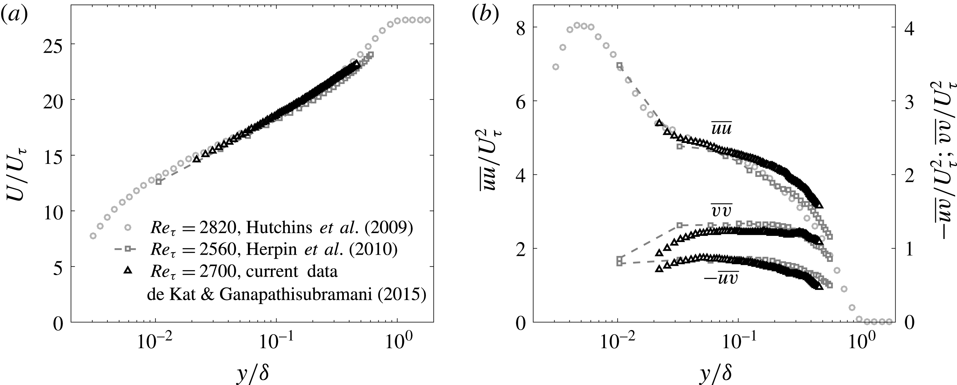
The resulting boundary-layer mean velocity and Reynolds stresses agree with previous studies at comparable Reynolds number (figure 1: Hutchins et al.
Reference Hutchins, Nickels, Marusic and Chong2009, and Herpin, Stanislas & Soria Reference Herpin, Stanislas and Soria2010). The observed overestimate of
 $\overline{uu}$
from the current dataset in comparison with measurements from the literature can be explained as differences in the level of free-stream turbulence intensity in the different facilities where experiments were performed. In particular, while the present dataset was obtained from measurements in a water tunnel, the datasets by Hutchins et al. (Reference Hutchins, Nickels, Marusic and Chong2009) and Herpin et al. (Reference Herpin, Stanislas and Soria2010) come from measurements in wind tunnels, which are typically characterized by lower levels of free-stream turbulence intensity.
2.1 Method for identification and tracking of intense momentum transport events
The main subjects of the present investigation are the intense Reynolds-stress events that populate the turbulent boundary layer. They are detected and statistically characterized in terms of extension, average intensity, and position of their weighted centroids. From the time-resolved data, the events are tracked across the time, which enables us to obtain the instantaneous local velocities of each event. In this section, we describe the method used for identification and tracking of the intense momentum transport events.
The noise in the PIV data was attenuated a posteriori by applying a regression filter, before calculating the Reynolds stress. The filtering of the data was performed both in time and in space. The filter replaces the value measured experimentally in a certain point of the domain, with the value obtained in the same point by least-squares fitting a polynomial function of the second order in
 $x$
(streamwise direction) and
 $y$
(wall-normal direction), and of the first order in the third dimension (time), in a
 $5\times 5\times 3$
neighbourhood around the point. Details on this regression filter are given by Elsinga et al. (Reference Elsinga, Adrian, van Oudheusden and Scarano2010). From these filtered velocity vector fields we obtained the instantaneous RSS fields (
 $uv$
). The criterion used for the detection of the intense transport events is analogous to Willmarth & Lu (Reference Willmarth and Lu1972), and is the following:
 $$\begin{eqnarray}|uv(x,y)|>H|\overline{uv}(y)|,\end{eqnarray}$$
where
 $uv(x,y)$
is the local Reynolds stress,
 $\overline{uv}(y)$
is the Reynolds stress averaged over the streamwise direction (figure 1), and
 $H$
is a coefficient. Analogous to previous studies on intense transport events, inhomogeneities along the streamwise direction are not accounted for in the identification criterion adopted in the present work (2.1). The levels of inhomogeneity of
 $\overline{uv}(y)$
along
 $x$
were checked in proximity to the wall (at
 $y^{+}<180$
), and found to be mild. In addition, the connected regions satisfying the criterion in (2.1) should be at least composed of nine points in order to be identified and tracked. This has the aim of discarding excessively small transport events, which can be the result of measurement error (spurious vectors or outliers, Adrian & Westerweel Reference Adrian and Westerweel2011).
The algorithm for the tracking of the intense transport events is also described in the present section. Two intense transport events
 $ev_{1}$
and
 $ev_{2}$
that are identified at two consecutive time instants, with
 $ev_{1}$
earlier in time with respect to
 $ev_{2}$
, are considered to be the same intense event if the following relationship holds:
 $$\begin{eqnarray}d_{\mathit{cent}}<D_{\mathit{box}},\end{eqnarray}$$
where
 $d_{\mathit{cent}}$
is the distance between the centroids of
 $ev_{1}$
and
 $ev_{2}$
, and
 $D_{\mathit{box}}$
is the diagonal of the smallest rectangle including all the points of
 $ev_{1}$
. As it can be noticed, the tracking algorithm presented here is based on the size of the first event, and on the distance between the centroids of
 $ev_{1}$
and
 $ev_{2}$
. The criterion is thus less stringent than the one used by Lozano-Durán & Jiménez (Reference Lozano-Durán and Jiménez2014) in their study, in that it is not necessary to have overlap between
 $ev_{1}$
and
 $ev_{2}$
in order to consider these to be the same event. The present tracking algorithm is applied to every intense transport event
 $ev_{2}$
located downstream with respect to an intense transport event
 $ev_{1}$
. This means that the connection between two or more
 $ev_{1}$
events with only one
 $ev_{2}$
event constitutes a merging of events, while when one
 $ev_{1}$
is connected with two or more
 $ev_{2}$
events, a splitting of events is observed.
Boundary layer statistics. (a) Mean profile, (b) Reynolds stresses.

3 Reynolds shear stress
In the first part of this section, the analysis is based on identification and tracking of the intense RSS events. The second part of the section is aimed at quantifying the contributions of the different frequencies and wavenumbers of the RSS fluctuations, and at assessing the spatial extent of the RSS structure at different wall-normal locations. These investigations are based on power spectra and autocorrelation functions.
3.1 Intense RSS events
In tracking the intense events contributing to the RSS, we distinguish between negative (
 $Q^{-}$
) and positive (
 $Q^{+}$
) events. The intense events were detected with the criterion reported in § 2.1 (2.1). A coefficient
 $H=1.8$
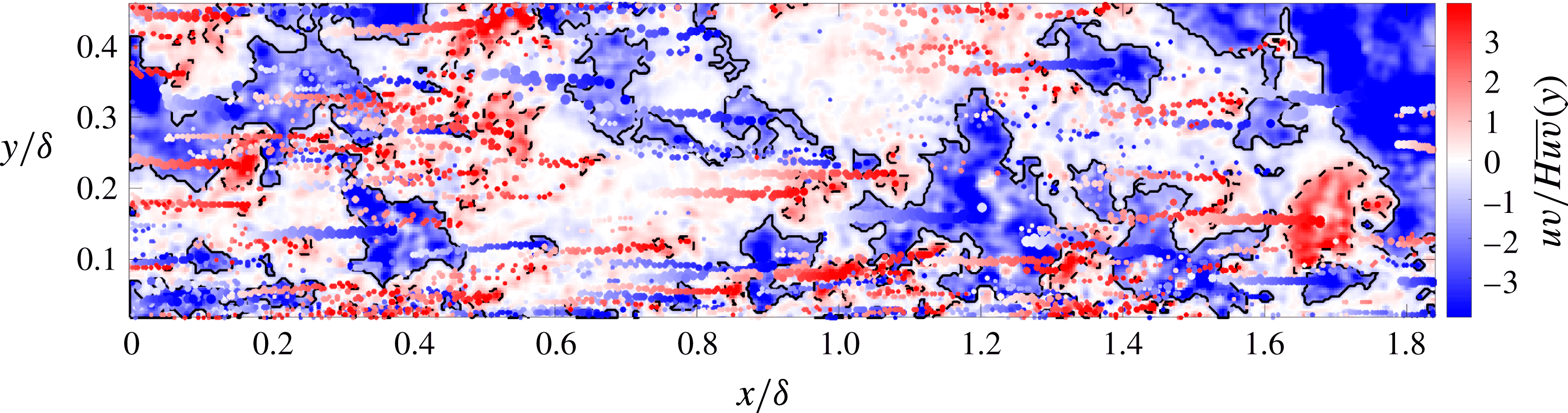
was chosen to identify the intense transport events. Supplementary movie 1, available at https://doi.org/10.1017/jfm.2017.841, shows the time evolution of the detected intense RSS events. Black continuous lines mark intense
 $Q^{-}$
events, while black dashed lines mark intense
 $Q^{+}$
events. Spots of different sizes and shades highlight the time development of weighted centroids of the intense events. In particular, the size of each spot is proportional to the extension of the related event, while its shade reflects the time span at which a given weighted centroid was detected. The time span covered in this movie is
 $1.33\unicode[STIX]{x1D6FF}/U_{\infty }$
. This means that the real flow is approximately 140 times faster than in the movie. The first snapshot of supplementary movie 1 is given in figure 2, where the time evolution of the weighted centroids of the intense quadrant events is also given. As it can be seen, the
 $Q^{+}$
events appear to be smaller and less numerous than the
 $Q^{-}$
events. Both the observations are confirmed when examining all the detected events. The total number of detected
 $Q^{-}$
events is
 $3.5\times 10^{6}$
, while the detected
 $Q^{+}$
events are
 $3.22\times 10^{6}$
.
Snapshot of positive and negative quadrant events of the RSS. Black dashed lines mark intense
 $Q^{+}$
events, while black continuous lines mark intense
 $Q^{-}$
events, both identified with the criterion shown in (2.1). Spots of different sizes and shades mark the time evolution of the weighted centroids of the intense events.

From the analysis of the intense RSS events, we found that the average of the total area of the
 $Q^{+}$
events is 11 % of the whole extension of the measurement plane, whereas the total area of the
 $Q^{-}$
events is 29 % of the whole extension of the measurement plane. The intense
 $Q^{+}$
events account for 70 % of the total positive quadrant RSS, while the intense
 $Q^{-}$
events accounts for 87 % of the total negative quadrant RSS. This is evidence that the largest contributions in terms of RSS are located within intense, intermittent, and physically small events, and that it is strongly inhomogeneous. Moreover, it is possible to quantify the distinct contributions to the total RSS given by the negative and the positive events.
 $Q^{-}$
events account for 150 % of the total RSS, and the
 $Q^{+}$
events account for only
 $-50\,\%$
of the total RSS. This shows that the largest contribution to the total RSS comes from
 $Q^{-}$
events, i.e. from ejection and sweep events. Therefore, it is of interest to separate the contributions of ejection and sweep events to the total RSS. We found that 53 % of the negative RSS comes from ejection events, while 47 % of the negative RSS from sweep events, which respectively accounts for 40 % and 35 % of the total RSS. These results are consistent with the measurements by Nagano & Tagawa (Reference Nagano and Tagawa1998) in a turbulent pipe flow, also reported in Wallace (Reference Wallace2016). As observed in several analyses from the literature (Robinson Reference Robinson1991; Lozano-Durán et al.
Reference Lozano-Durán, Flores and Jiménez2012; Lozano-Durán & Jiménez Reference Lozano-Durán and Jiménez2014, among others), the individual contributions of each of the quadrant events to the total RSS strongly depends on the wall-normal location. Therefore, it is of interest to quantify the relationship between the intensity of a RSS event, and its wall-normal position within the boundary layer. This analysis is performed for the intense positive and negative events, without distinguishing between ejection and sweep events, which are examined in detail in § 4.
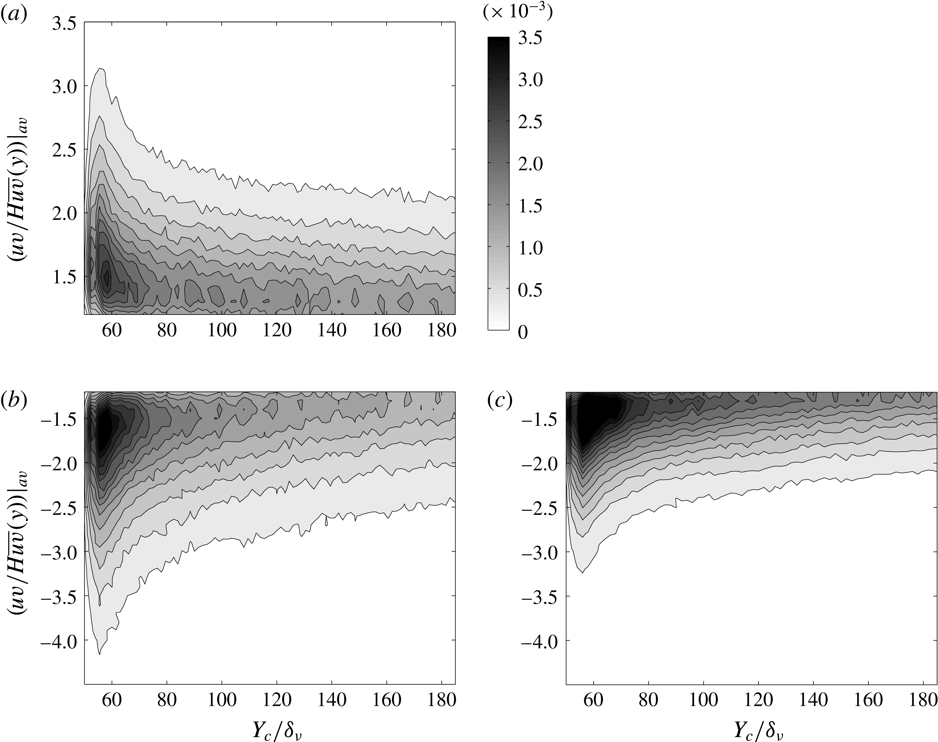
Joint probability density function between intensity of events and their wall-normal locations for a threshold of
 $H=1.8$
for positive (a) and negative (b) events and for a higher value of threshold
 $H=3.0$
, only for negative events (c).

Figure 3 shows joint probability density functions (j.p.d.f.s) between the intensity of the intense RSS events and the wall-normal position of their centroids
 $Y_{c}$
, non-dimensionalized by
 $\unicode[STIX]{x1D6FF}_{\unicode[STIX]{x1D708}}=\unicode[STIX]{x1D708}/U_{\unicode[STIX]{x1D70F}}$
. The RSS events are separated into positive (top) and negative (bottom) events. A coefficient
 $H=1.8$
was chosen to detect the intense events, while a higher threshold
 $H=3$
was applied to detect more intense
 $Q^{-}$
events. A total number of
 $3.22\times 10^{6}$
 $Q^{+}$
events was detected, while
 $3.50\times 10^{6}$
and
 $2.96\times 10^{6}$
 $Q^{-}$
events were identified using the coefficients
 $H=1.8$
and
 $H=3$
, respectively. Figure 3(a) shows that the
 $Q^{+}$
events are more uniformly distributed across the wall-normal positions within the flow, while in figure 3(b) the
 $Q^{-}$
events tend to be more preferentially located in proximity to the wall. The intensity of the events located at the wall is larger for the
 $Q^{-}$
events, as can be seen in figure 3(b). The range of intensities of
 $Q^{-}$
events decreases with increasing wall-normal distance, while this transition is smoother for
 $Q^{+}$
events. A similar trend was observed by Morrill-Winter et al. (Reference Morrill-Winter, Philip and Klewicki2017).
For
 $H=3$
, the distribution of intense
 $Q^{-}$
events across the wall-normal locations, presented in figure 3(c), appears to be similar to the one in figure 3(b). The range of intensities at the wall is smaller for
 $H=3$
. This is expected, and it can be explained with the choice of a larger threshold in the detection criterion. However, the qualitative shape of the j.p.d.f. seems to be insensitive to an almost 50 % increase in the coefficient of the threshold (from
 $H=1.8$
to
 $H=3$
). This is consistent with the observations of Lozano-Durán et al. (Reference Lozano-Durán, Flores and Jiménez2012), who reported that the results are qualitatively similar for large variations of the coefficient in the detection criterion.
This section establishes that the TBL data presented here have characteristics that are similar to other previous studies on analogous flows when it comes to RSS. Furthermore, it validates our method for identifying and quantifying these intense RSS events. In the following subsections, we will examine the data using spectral and spatial correlation methods in order to identify the space–time/Fourier domain evolution of these events.
3.2 Wavenumber–frequency power spectra of the RSS fluctuations
The RSS fluctuations can be decomposed into contributions of the different wavenumbers and frequencies, to quantify the scale dependence of fluctuations in momentum transport events. Power spectra were obtained from the time-resolved RSS
 $uv$
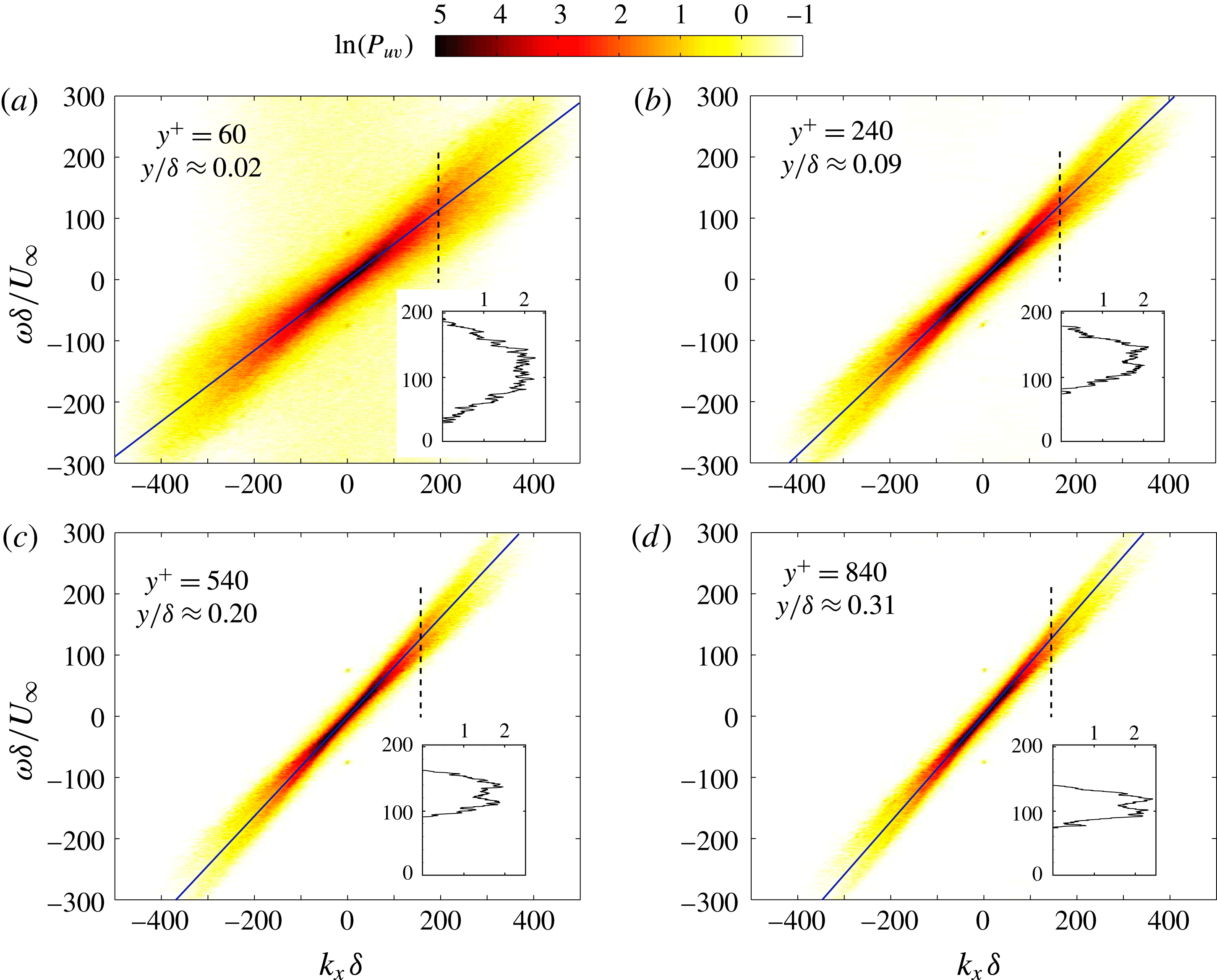
, calculated from the PIV velocity vector fields. The RSS data were organized in an array collecting the time and streamwise space evolution of the RSS, at a given wall-normal location. The average was subtracted from this array of the RSS distribution, to obtain a field of RSS fluctuations, which was Hanning-filtered before calculating the power spectra. In figure 4, the wavenumber–frequency power spectral density of the RSS fluctuations is presented, at four different wall-normal distances:
 $y^{+}=60$
(
 $y/\unicode[STIX]{x1D6FF}\approx 0.02$
);
 $y^{+}=240$
(
 $y/\unicode[STIX]{x1D6FF}\approx 0.09$
);
 $y^{+}=540$
(
 $y/\unicode[STIX]{x1D6FF}\approx 0.20$
); and
 $y^{+}=840$
(
 $y/\unicode[STIX]{x1D6FF}\approx 0.31$
). On the
 $x$
and
 $y$
axes, the angular wavenumber and the angular frequency are reported, respectively, where the meaning of the adopted symbols is the same as in de Kat & Ganapathisubramani (Reference de Kat and Ganapathisubramani2015b
).
Wavenumber–frequency power spectral density of the RSS fluctuations, at different wall-normal distances. Continuous lines represent the local average streamwise velocity. Plots in the insets show sections of the power spectra along the vertical dashed lines.

Figure 4 shows that a large range of time and length scales of turbulence is involved in the momentum transport in proximity to the wall. However, when moving away from the wall, a decreasing area of the power spectrum contributes to the RSS fluctuations. A region of values between
 $-1$
and 0 on a logarithmic scale exists in the wavenumber–frequency spectrum at
 $y^{+}=60$
, which is equivalent to values in the range
 $1/\text{e}=0.368$
and 1. This represents a mild broadband noise affecting the measurement. A common characteristic to each of the four spectra presented in figure 4 is their diagonal-stripe-like shape. This particular shape indicates that the contribution of a given wavenumber is preferentially associated with a narrow frequency band. This feature can be interpreted as an indication of the local characteristic wave velocities (
 $U_{A}$
) of the RSS fluctuations, at different wall-normal locations.
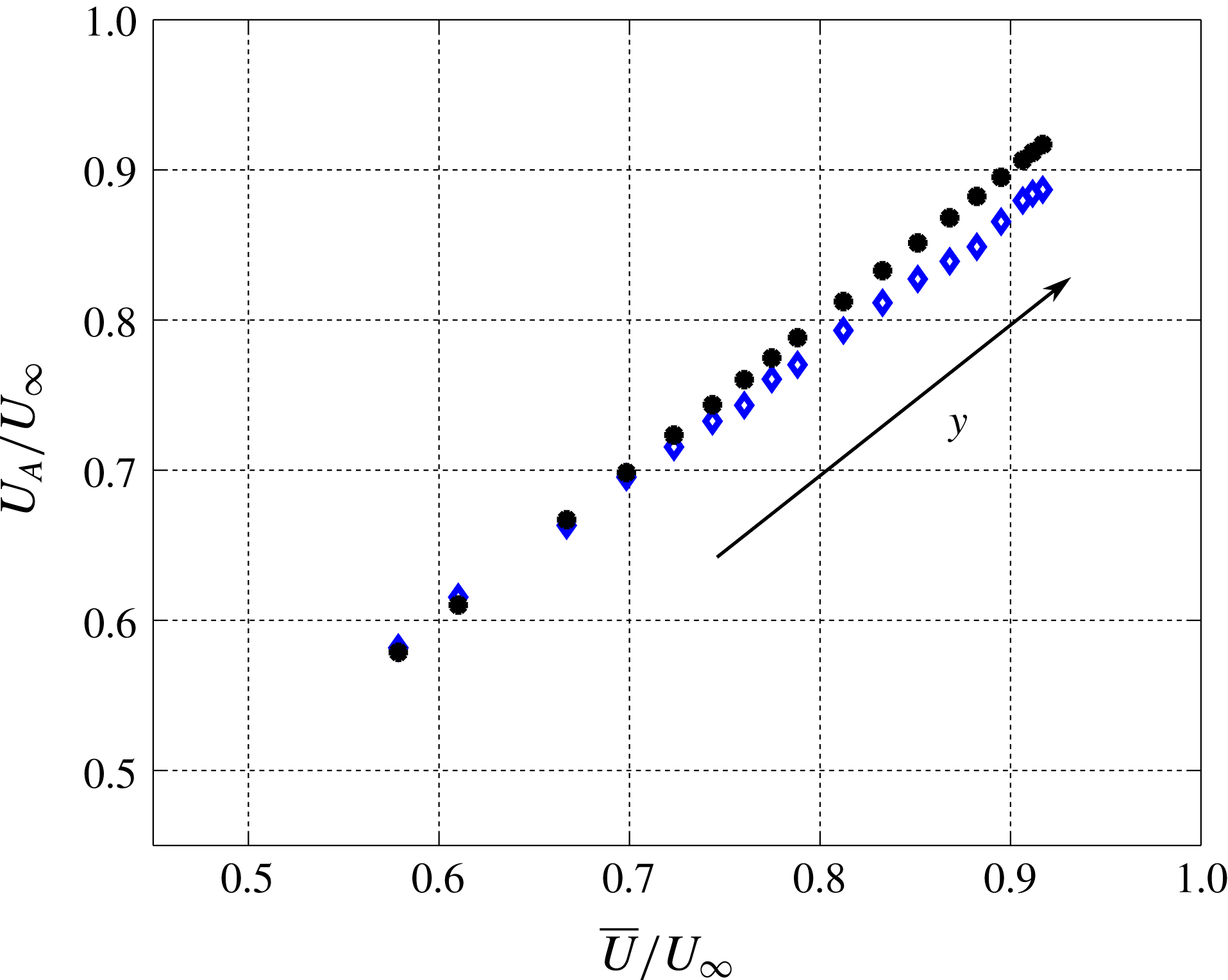
Characteristic wave velocities of the RSS (blue diamond, ♢) at different wall-normal locations, calculated from the wavenumber–frequency power spectra. Black filled circles (●) indicate the average streamwise velocity.

The characteristic wave velocities of the RSS events can be estimated from each wavenumber–frequency power spectrum, at the full range of different wall-normal locations available from the experimental dataset (
 $y^{+}=50$
–1280). The wavenumber–frequency spectra were thresholded at thirteen values, at intervals of 0.25, in the range
 $0.5\leqslant \ln (P_{uv})\leqslant 3.5$
. At each contour level of the wavenumber–frequency power spectrum, an ellipse was fitted to the points delimiting the edge of the contour level. A linear least-squares fitting method was employed, which optimizes the squared sum of orthogonal distances from the points to the fitted ellipse. The initial guess is calculated by a linear least-squares routine, using the ‘Bookstein constraint’ (see Gander, Golub & Strebel (Reference Gander, Golub and Strebel1994) for further detail). A fitting ellipse is defined by its centre, major and minor axes, and rotation angle. The average of the rotation angles of each fitted ellipse is taken as an estimate for the characteristic wave velocity of the RSS events, at a given distance from the wall.
The result of above-described procedure is presented in figure 5. Blue diamonds (♢) mark the characteristic wave velocities of the RSS, while filled circles (●) represent the average streamwise velocity of the flow. The RSS wave velocities are marginally faster than the mean velocity close to the wall. We expect wave velocities faster than the relative mean streamwise velocities at
 $y^{+}<50$
. This trend is not well captured due to the limited spatial resolution. However, the wave velocities of the RSS events are slower than the mean streamwise velocity farther away, and this trend is clear from the results presented in figure 5. Overall, the trend of wave velocities presented in figure 5 is consistent with the findings by del Álamo & Jiménez (Reference del Álamo and Jiménez2009) on a DNS channel flow (figures 1 and 2), even if their estimate was based on ensemble averages of single Fourier modes’ time derivatives.
These observations suggest that there exists a certain point where
 $U_{A}=\overline{U}\approx 0.65U_{\infty }$
, which is approximately in the middle of the log region where the RSS events are ‘passively’ carried by the mean flow. Beyond this location, the advection speeds appears to be lower than the mean velocity. This trend is similar to the advection speed of large-scale structures described by del Álamo et al. (Reference del Álamo, Jiménez, Zandonade and Moser2006). Therefore, the above method appears to bias the advection speed towards larger scales of the flow. However, the instantaneous events of shear stress do not extend over large spatial scales. They are more compact in size. Therefore, this bias towards the large-scale advection velocity is more likely due to the advection of a collection of RSS events that are aligned in the streamwise direction. This collection of intense RSS events advect together with a similar speed, which is consistent with the presence of hairpin packet type event. Any difference in the relative speed between adjacent RSS events will result in a dispersion of energy at that particular length scale related to these events. This perhaps explains the diffusion of spectral energy into different neighbouring frequencies.
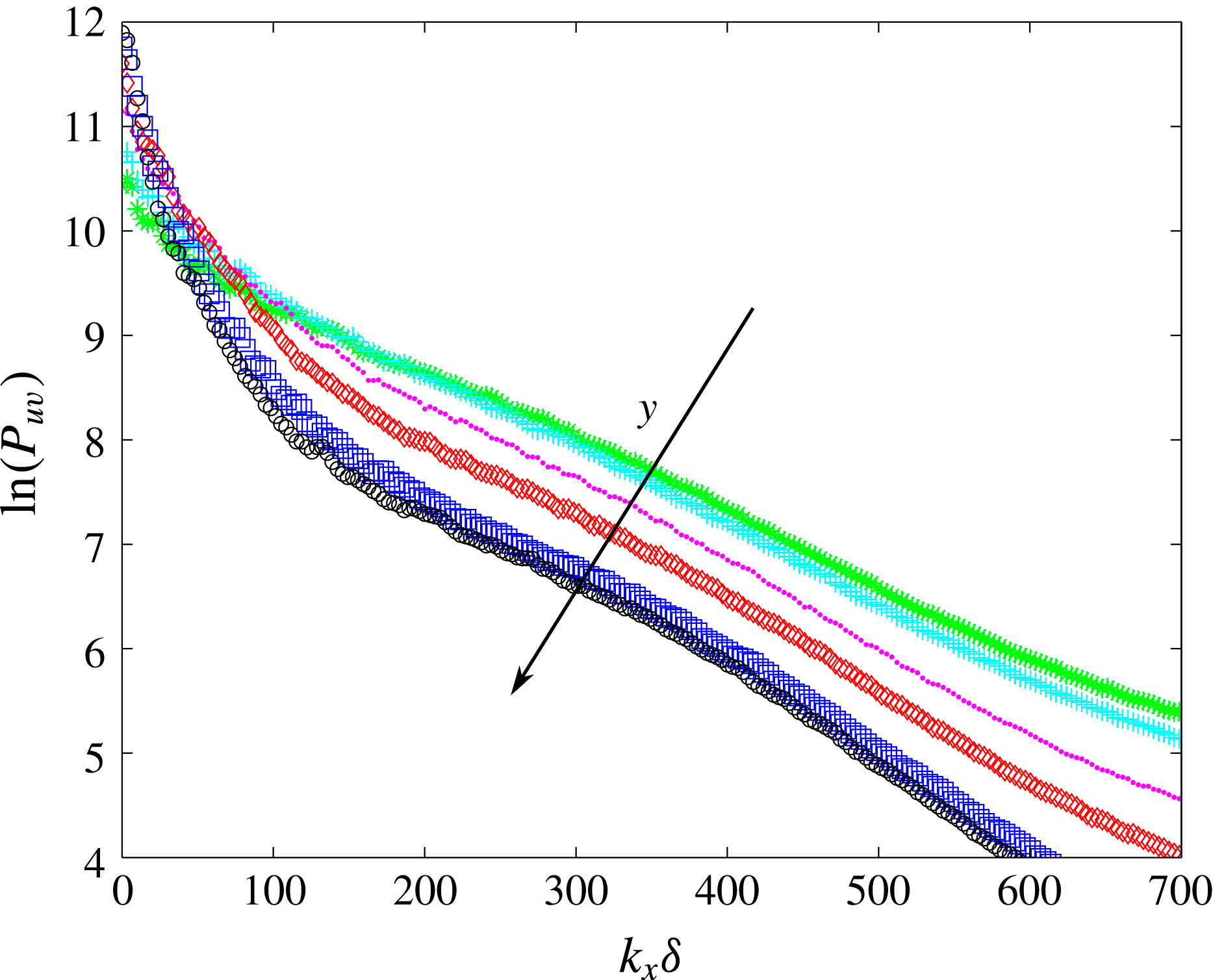
Power spectra of the RSS, at different wall-normal distances (colours in the online version), green *:
 $y^{+}=60$
, cyan
 $+$
:
 $y^{+}=80$
, magenta ●:
 $y^{+}=140$
, red ♢:
 $y^{+}=240$
, blue ▫:
 $y^{+}=540$
, black ○:
 $y^{+}=840$
.

From figure 4, we can observe that at a given wavenumber the spectra exhibit two local maxima. This means that a given wavenumber can be associated with two distinct frequency bands in the wavenumber–frequency domain. This is in addition to the spectral spillage to neighbouring frequencies at those bands. The described two-peak structure of the power spectra is made more evident by the insets reporting sections along the vertical dashed lines. A moving average filter was applied to the obtained line plots, with a window size of
 $2.3\unicode[STIX]{x1D714}\unicode[STIX]{x1D6FF}/U_{\infty }$
. These observations suggest that the RSS could be characterized by two distinct bands of characteristic wave velocities. In figure 4, the two characteristic wave velocities of the RSS are bisected by the local average velocity. Therefore, there are two types of distinct events contributing energetically to the RSS, each of them with a characteristic wave velocity. The wavenumber–frequency spectra also reveal that in proximity to the wall, the RSS is characterized by a larger range of wave velocities than far from the wall. It appears that the two characteristic wave velocities deviate progressively less from the associated average streamwise velocity at growing distances from the wall. Therefore, the characteristic wave velocities of the two distinct events contributing to the RSS tend to match more closely with each other, and they appear to converge towards the average local streamwise velocity for increasing distances from the wall.
Figure 4 also shows that both the high frequencies and the high wavenumbers of the spectra tend to progressively contribute less when the distance from the wall increases. This suggests that larger sizes in streamwise direction and longer lifetimes characterize the structure of the RSS at increasing wall-normal locations. This is consistent with the observations of del Álamo et al. (Reference del Álamo, Jiménez, Zandonade and Moser2006), Flores & Jiménez (Reference Flores and Jiménez2010), and Lozano-Durán & Jiménez (Reference Lozano-Durán and Jiménez2014) in a DNS channel flow, with the attached-eddy hypothesis of Townsend (Reference Townsend1961), and with the recent hot-wire measurements of Morrill-Winter et al. (Reference Morrill-Winter, Philip and Klewicki2017) in TBLs. Also, LeHew, Guala & McKeon (Reference LeHew, Guala and McKeon2013) found that the lifetimes of the swirling structures increase with the wall distance in a TBL. The evidence gained from the wavenumber–frequency spectra of figure 4 can be corroborated when looking at the power spectra in figure 6, which were obtained by summing the contributions of the different frequencies. A clear trend can be observed, with the high wavenumbers (short wavelengths) losing spectral relevance for increasing distances from the wall. Similarly, the spectral content of the low wavenumbers (long wavelengths) grows with increasing distance from the wall. The described change in the composition of the spectrum with the wall-normal location becomes less significant in the range of wall-normal distances
 $240<y^{+}<540$
. If we compare the wavenumber power spectra at
 $y^{+}=540$
and
 $y^{+}=840$
, we can notice that they nearly overlap. Similarly, wavenumber power spectra calculated at wall-normal distances higher than
 $y^{+}=840$
, which have not been reported in figure 6, show modest deviations from the spectra at
 $y^{+}=540$
and
 $y^{+}=840$
.
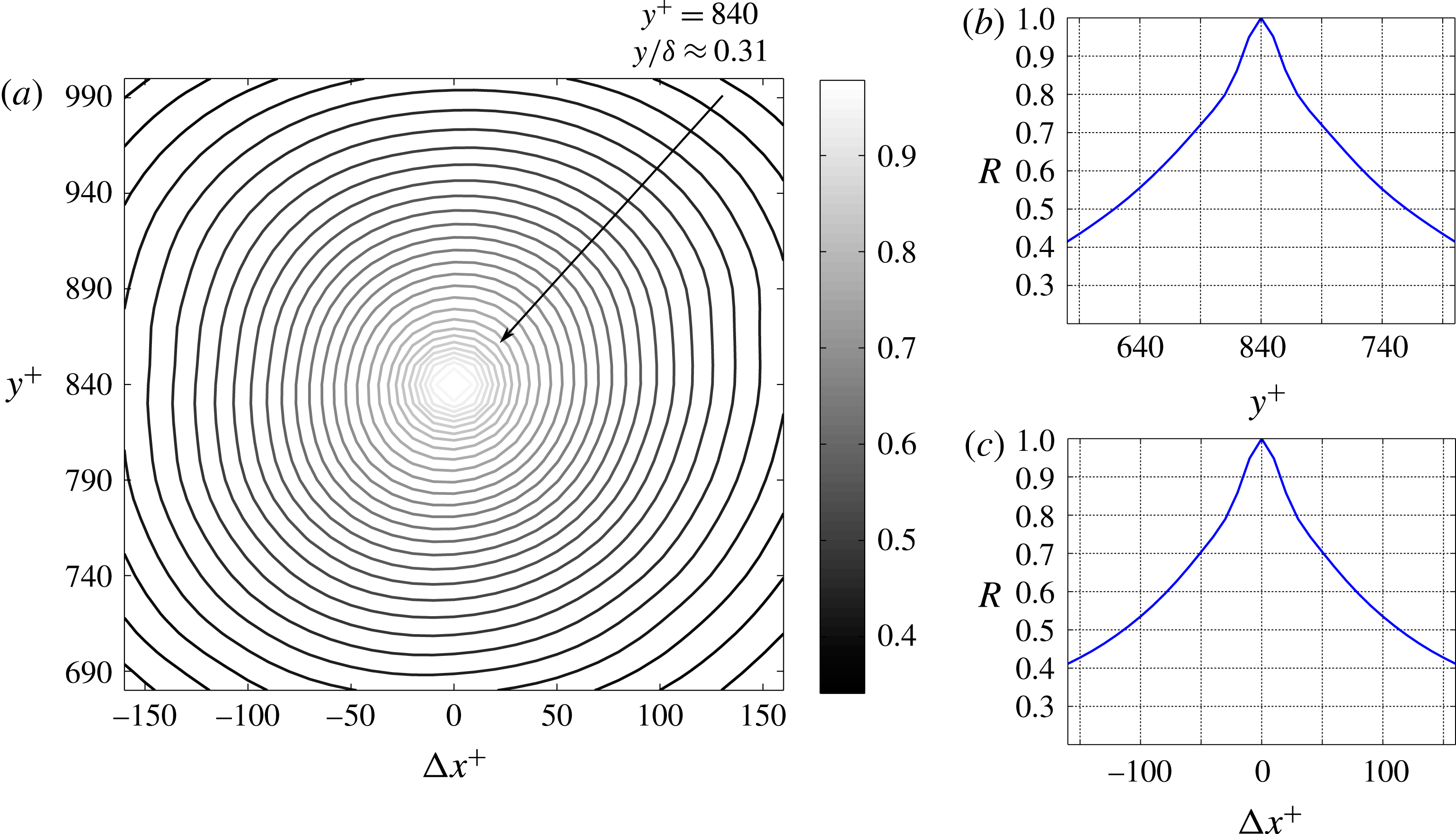
3.3 Autocorrelation maps of the RSS
The analysis of the spectra conducted above suggests that the streamwise extent of the RSS structure increases with the distance from the wall. This finding is consistent with the attached-eddy hypothesis proposed by Townsend (Reference Townsend1961). In the following, the characteristic size of the RSS structure is assessed at different wall-normal locations by correlating the
 $uv$
signal at a given distance from the wall with the
 $uv$
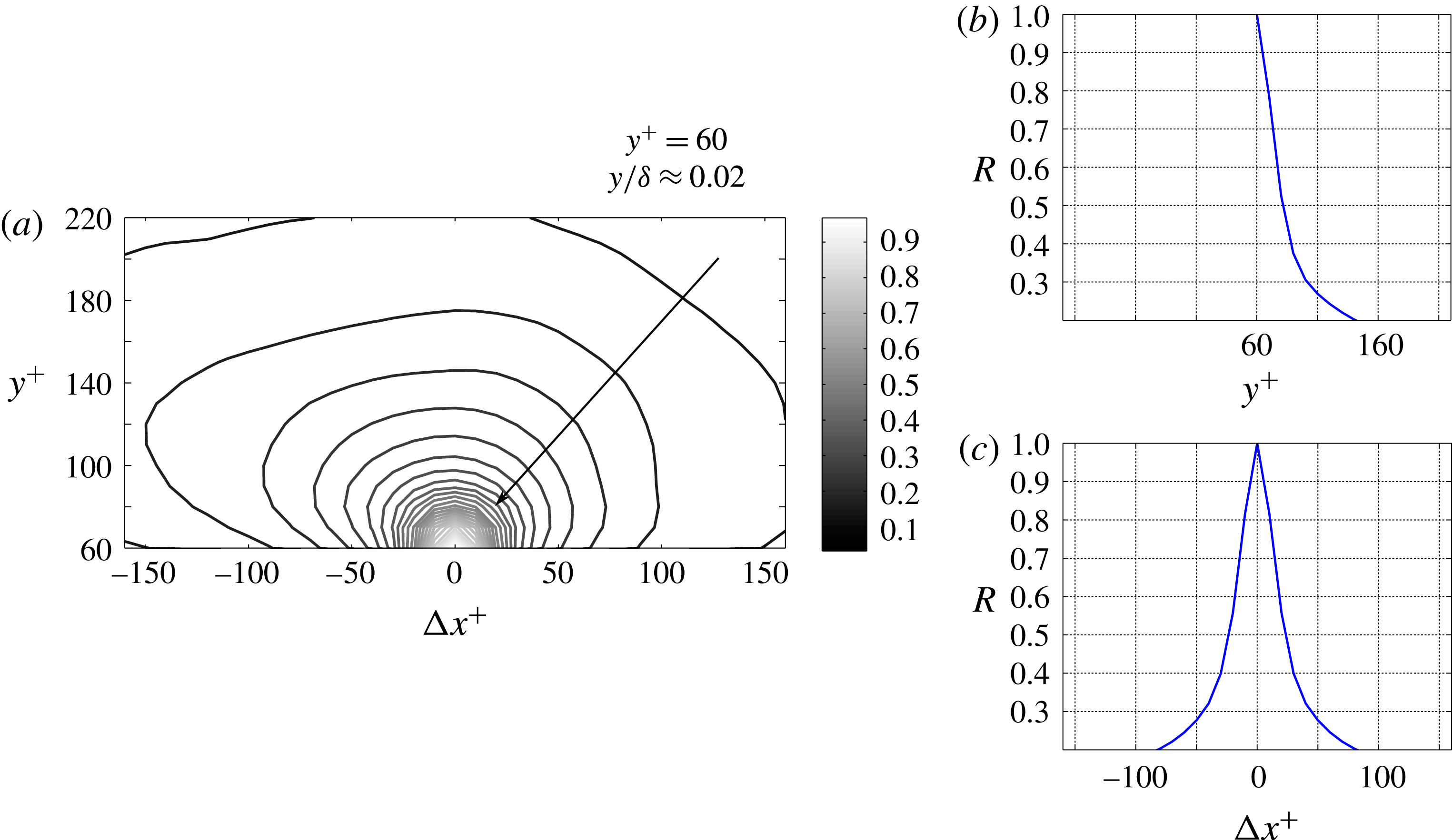
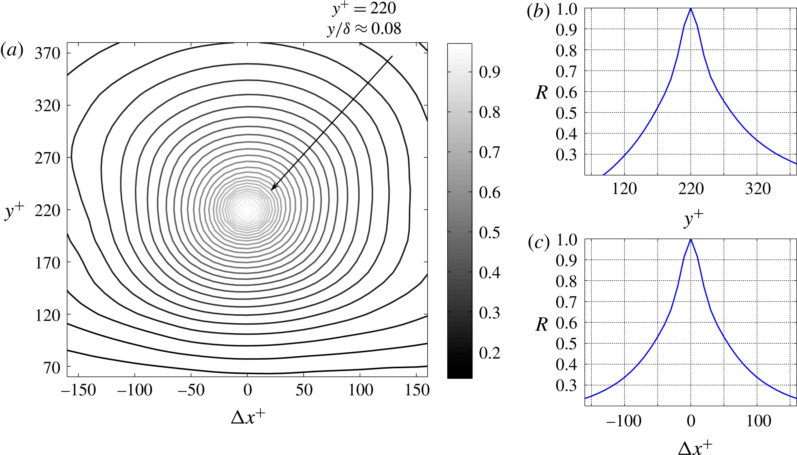
signals at different distances from the wall. The resulting correlation map is normalized by the respective autocorrelation coefficient at a given wall distance, at zero shift. The autocorrelation maps of the RSS at
 $y^{+}=60$
,
 $y^{+}=220$
, and
 $y^{+}=840$
are presented in figures 7(a), 8(a), and 9(a), respectively.
Beside the autocorrelation maps, sections of the autocorrelation coefficients along the wall-normal and streamwise directions through the origin are shown. In figure 7(a), we can observe that the autocorrelation function of the RSS is not symmetric with respect to the axis
 $[\unicode[STIX]{x0394}x^{+}=0,y^{+}]$
. In particular, higher correlation coefficients are obtained for negative streamwise shifts
 $\unicode[STIX]{x0394}x^{+}$
and for increasing wall-normal locations. This suggests that, at
 $y^{+}=60$
, the RSS structure resembles a comet, with an elongated trailing edge, and a rounded leading edge. At
 $y^{+}=220$
, the described behaviour is still evident, even if less significant, as it can be seen in figure 8(a). In particular, the autocorrelation coefficients are larger for
 $y^{+}>220$
, while for wall-normal locations lower than
 $y^{+}=220$
they tend to decrease more quickly to zero. Similarly, for positive wall-normal displacements, larger autocorrelation coefficients can be observed for negative
 $\unicode[STIX]{x0394}x^{+}$
, which produces the observed elongated shape in the autocorrelation map.
At increasing distances from the wall, the shape of the RSS structure tends to be more circular. At
 $y^{+}=840$
, figure 9(a), there is no evidence left of the skewed shape that characterizes the RSS structure in proximity to the wall. Instead, the autocorrelation map exhibits a uniform dropoff for increasing distances from the origin, independent of direction.
Autocorrelation coefficient map of the RSS, at
 $y^{+}=60$
(a). Sections along the wall-normal (b) and streamwise (c) directions of the autocorrelation coefficients map as presented in (a).

Autocorrelation coefficient map of the RSS, at
 $y^{+}=220$
(a). Sections along the wall-normal (b) and streamwise (c) directions of the autocorrelation coefficients map as presented in (a).

Autocorrelation coefficient map of the RSS, at
 $y^{+}=840$
(a). Sections along the wall-normal (b) and streamwise (c) directions of the autocorrelation coefficients map as presented in (a).

To assess the size of the RSS structure at different wall-normal locations the profiles of autocorrelation maps are thresholded. At
 $R=0.5$
, the characteristic streamwise extent of the RSS structure at
 $y^{+}=60$
is approximately 50 wall units (figure 7
c). Due to the lack of experimental data at wall-normal locations
 $y^{+}<60$
, only the correlation coefficients were obtained for
 $y^{+}>60$
. The characteristic wall-normal extent of the RSS structure at
 $y^{+}=60$
is approximately 50 wall units, see figure 7(b). Similarly, the characteristic streamwise extent of the RSS structure at
 $y^{+}=220$
and
 $y^{+}=840$
can be estimated to be approximately 115 wall units (figure 8
c) and 225 wall units (figure 9
c), respectively. The characteristic wall-normal extent of the RSS structure at the same wall-normal distances is approximately 115 wall units, see figure 8(b), and 240 wall units, see figure 9(b), respectively. The assessment of the size of the RSS structure shows that the extents in the streamwise and wall-normal directions tend to be similar at a given distance from the wall, and that they both increase with increasing wall-normal location.
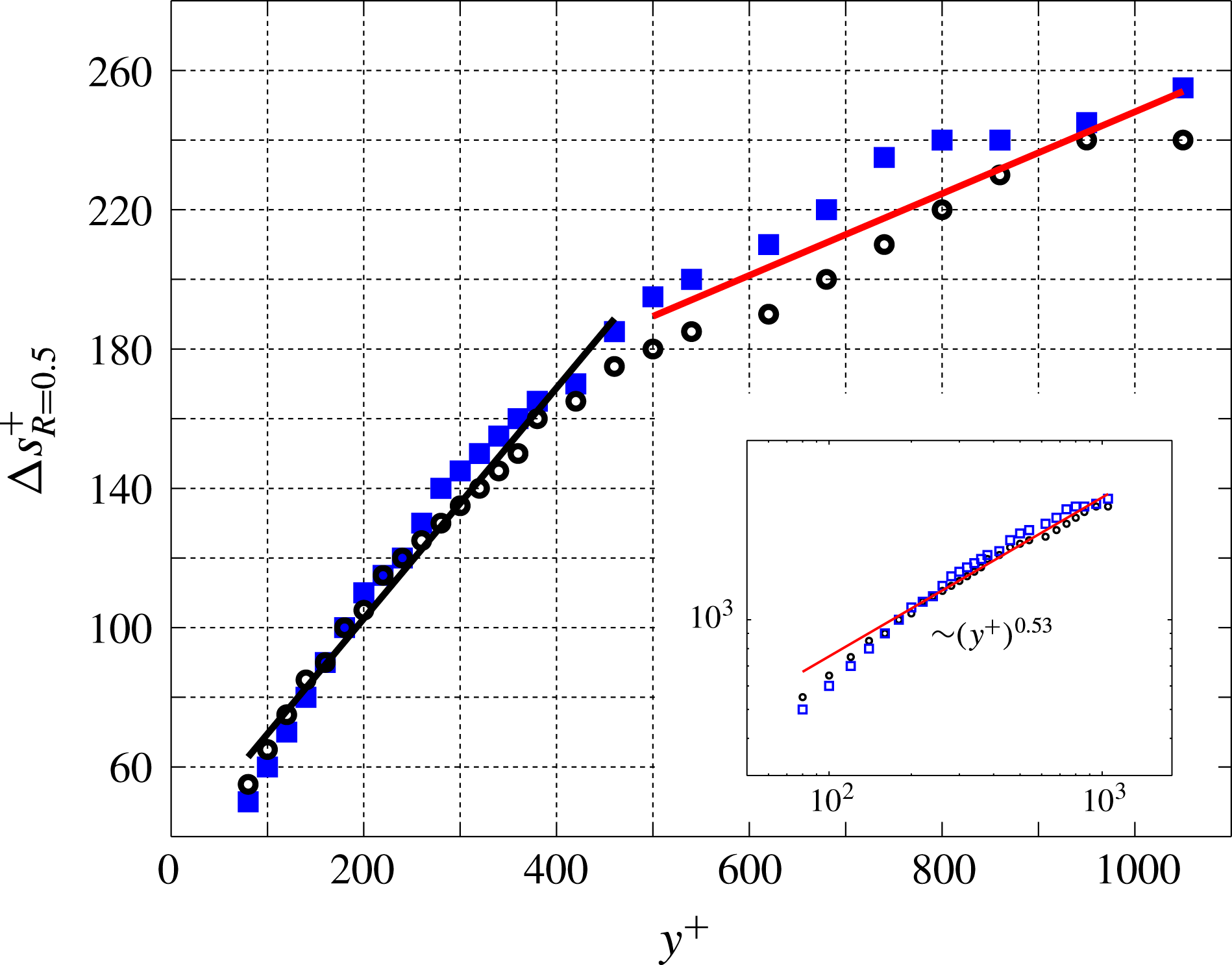
Setting a threshold of
 $R=0.5$
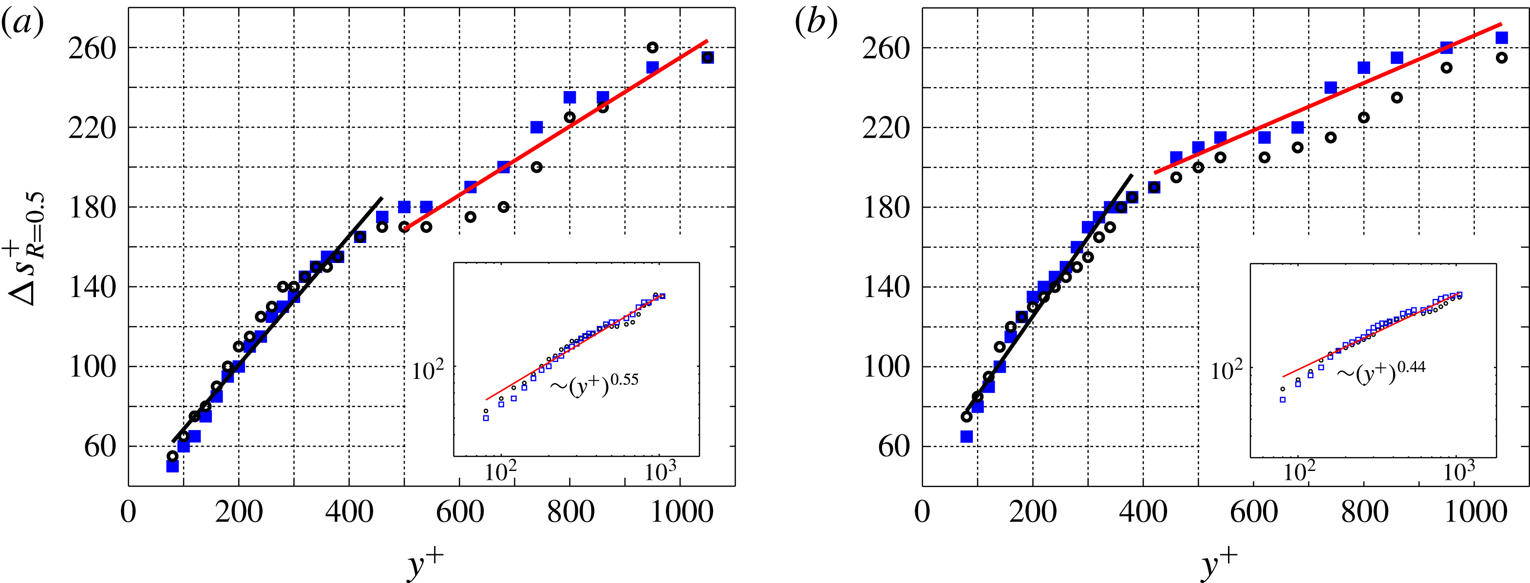
in the autocorrelation coefficients maps, the extent of the RSS structure along the wall-normal and streamwise directions can be assessed over the full range of wall-normal distances available. Figure 10 shows that the size of the RSS structure increases monotonically with the wall-normal location. The monotonic increase of the RSS size with the wall distance was also observed by Morrill-Winter et al. (Reference Morrill-Winter, Philip and Klewicki2017) from hot-wire anemometry measurements. The authors pointed at a self-similar structure that connects the geometry and dynamics of momentum transporting motions. For
 $y^{+}>250$
, the wall-normal extent of the RSS structure is larger than its streamwise extent. The difference between the wall-normal and the streamwise extent increases with the distance from the wall, till
 $y^{+}=750$
. For
 $y^{+}>750$
, this difference diminishes. In the range of wall-normal locations
 $y^{+}<450$
, a linear growth of the RSS size with the wall distance can be observed. At
 $y^{+}>450$
, a different linear trend characterizes the increase of the RSS size with the wall-normal distance, which has a lower slope than in the range
 $y^{+}<450$
. In figure 10, two lines of different colours mark the two different linear trends.
Characteristic extent of the RSS structure along the streamwise (empty circles, ○) and wall-normal (filled squares, ▪) directions, at different wall-normal distances. Results are based on autocorrelation maps, and
 $R=0.5$
was chosen as a threshold. In the inset, the same data are reported on a log–log plot, and an exponential fitting law is derived.

The change in the slope at
 $y^{+}=450$
can be explained as a predominance of the wall-attached RSS events over the wall-detached ones in the range
 $y^{+}<450$
, while at
 $y^{+}>450$
the wall-detached objects would be more numerous. This wall-normal location appears to be the outer edge of the log region (
 $y^{+}=450=y/\unicode[STIX]{x1D6FF}\approx 0.16$
). However, with the two-dimensional data in our possession it is not possible to support this explanation with a statistical quantification of the dominance of wall-attached events versus wall-detached ones. In the inset of figure 10, the same data are presented in a log–log plot, and an exponential fitting law is obtained. According to this result, an exponent of 0.53 governs the exponential relationship between the size and wall distance of RSS events. This trend is very similar to the scaling law characterizing the Taylor microscale in the logarithmic region of a TBL, which is of
 $(y^{+})^{0.5}$
. However, very recently, Morrill-Winter et al. (Reference Morrill-Winter, Philip and Klewicki2017) observed an exponential trend with an exponent of 0.382, and therefore significantly lower than the exponent obtained from the present work. They estimated the streamwise extent of the negative quadrant events from hot-wire anemometry, therefore from time series, and measured the average time where the
 $uv$
is negative. Regardless, what is clear is that the size of the RSS events increases rapidly within the log region and the rate of increase decreases in the outer wake.
Considering the modest contribution of the
 $Q^{+}$
events to the total RSS (25 %), the latter is largely represented by the
 $Q^{-}$
events, which can be distinguished into ejections and sweeps. As they are the main contributors to the total RSS, the following section examines in detail ejection and sweep events.
4 Ejection and sweep events
The present section focuses on ejection and sweep events. In the first part, their characterization is based on wavenumber–frequency power spectra and autocorrelation coefficients maps, similar to the analysis performed on the RSS. In the second part, intense ejection and sweep events are tracked across time. The analysis illustrated in the present section yields a statistical quantification of intensity, advection velocity, and size of ejections and sweeps, in relation to their wall-normal location.
4.1 Wavenumber–frequency power spectra of
 $Q^{-}$
fluctuations

Wavenumber–frequency power spectra enable one to quantify the spectral content of the different streamwise wavenumbers and frequencies at different wall-normal locations. The procedure to obtain these spectra of
 $Q^{-}$
fluctuations events is analogous to the one detailed in § 3 for the wavenumber–frequency power spectra of the RSS fluctuations. However, each value of the
 $uv$
field not corresponding to an ejection or a sweep event was set to zero, and the average value of the remaining
 $uv$
within each frame was subtracted. Setting to zero some values of the
 $uv$
field could produce an artificial increase of the resulting spectral content at high wavenumbers and frequencies. This issue was checked, and it was found that the additional spectral contributions consequent to this procedure were not significant, and that wavenumbers and frequencies that are multiples of the dominant ones are not excited. The spectral content of the dominant modes gets mildly dampened by this procedure, even though their dominance remains such.
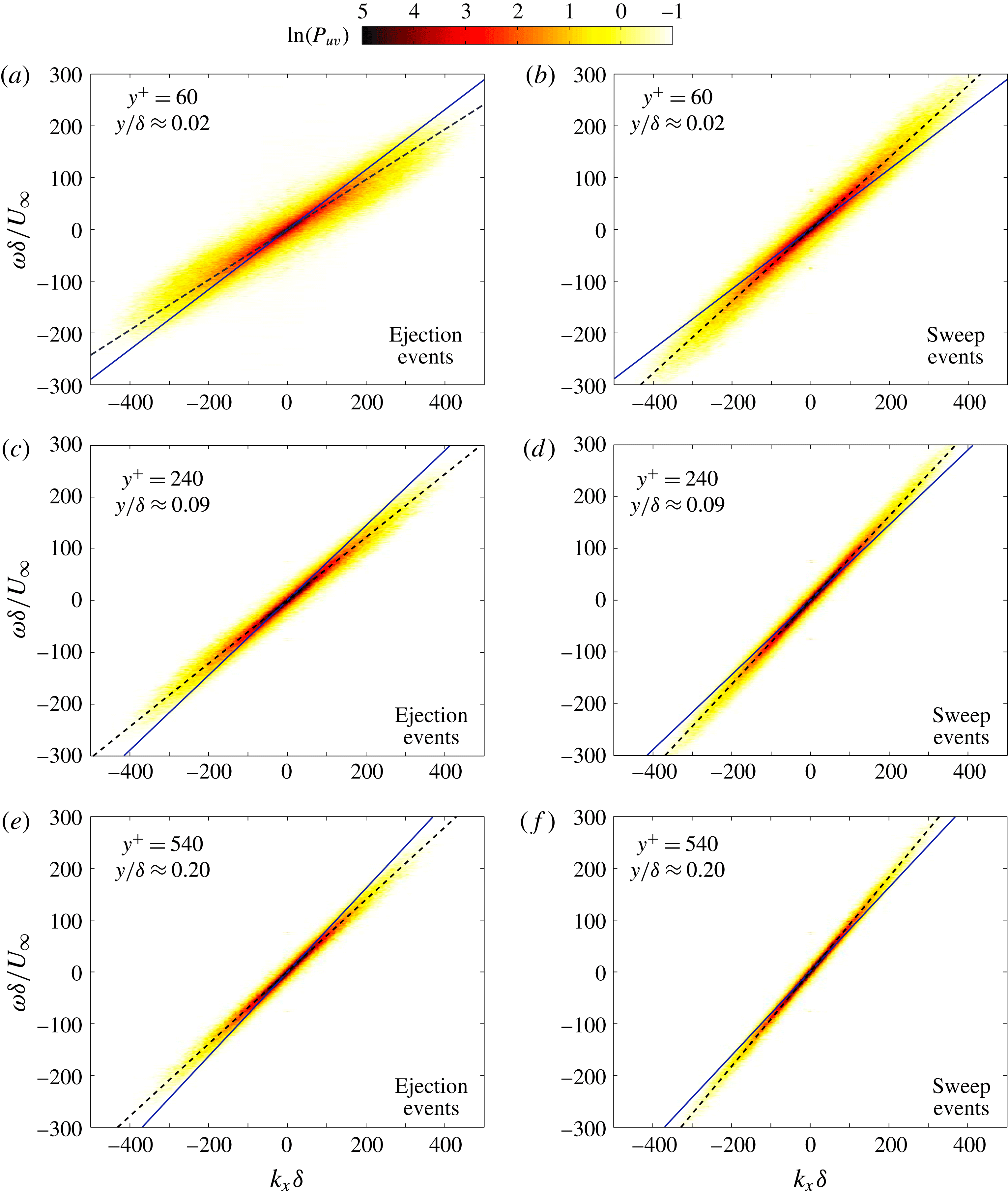
Wavenumber–frequency power spectral density of the ejection (a,c,e) and sweep (b,d,f) events, at different wall-normal locations. Continuous lines represent the local average streamwise velocity, while dashed lines indicate the local characteristic wave velocity.

Wavenumber–frequency power spectra of ejection events (panels a,c,e) and sweep events (panels b,d,f) are presented in figure 11, at
 $y^{+}=60$
,
 $y^{+}=240$
, and
 $y^{+}=540$
. Each spectrum has an elongated ellipse that is inclined along the advection diagonal. In contrast to the spectra of the RSS fluctuations (figure 4), only one distinct frequency band can be associated with a given wavenumber. A procedure similar to that illustrated in the previous section can be applied with the aim of obtaining an estimate of the local characteristic wave velocities (
 $U_{A}$
) at different wall-normal locations. The procedure is based on fitting ellipses to the points delimiting the edges of the different contour levels.
In figure 11, black dashed lines represent an estimate of the characteristic wave velocity obtained from this procedure, while blue continuous lines represent the local average streamwise velocity. Ejection events are characterized by wave velocities lower than the local average velocity of the flow (higher slope of the continuous lines), whereas sweep events are characterized by wave velocities higher than the local average velocity of the flow (higher slope of the dashed lines). This observation is in agreement with Lozano-Durán & Jiménez (Reference Lozano-Durán and Jiménez2014). Furthermore, the relative difference between the wave velocities of the
 $Q^{-}$
events and the local average velocity of the flow tends to diminish for increasing distances from the wall. At a given wavenumber, the range of frequencies carrying a significant contribution to the spectrum becomes smaller with the distance from the wall, consistent with the power spectra of the total RSS fluctuations (figure 4). It is important to notice that at
 $y^{+}=60$
, the contribution to the spectrum of the ejection events is contained in a larger range of frequencies than the spectral contribution of the sweep events, for a given wavenumber. This suggests that the ejection events are characterized by a larger range of wave velocities than the sweep events, at
 $y^{+}=60$
.
Farther from the wall, high wavenumbers and high frequencies (low wavelengths) tend to reduce their contribution to the spectrum. Instead, the spectral content of low wavenumbers and low frequencies (high wavelengths) grows, for increasing wall-normal locations. This suggests the
 $Q^{-}$
events are characterized by larger extensions in size and longer lifetimes at growing distance from the wall.
As already shown in § 3, the characteristic wave velocities can be estimated from each wavenumber–frequency power spectrum, at the full range of different wall-normal locations available from the experimental dataset. The procedure illustrated in the previous section is therefore extended to several wavenumber–frequency power spectra in the range of wall-normal locations
 $50y^{+}$
to
 $1280y^{+}$
.
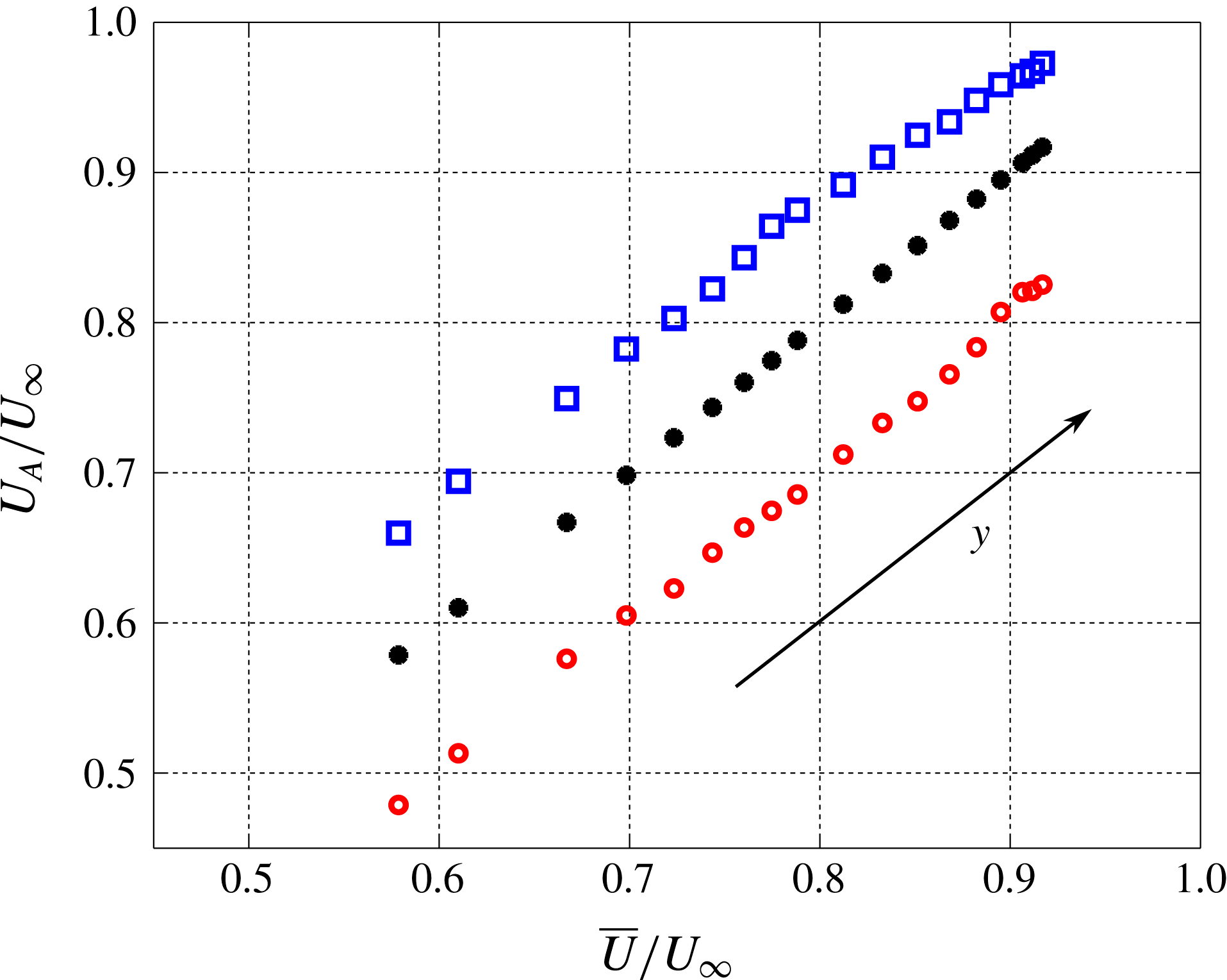
The result of this analysis is presented in figure 12. Red circles and blue squares mark the characteristic wave velocities of ejection (○) and sweep (▫) events, respectively. Filled circles (●) represent the average streamwise velocity of the flow. According to this analysis, the relative difference between wave velocities of the
 $Q^{-}$
events and the local average streamwise velocity decreases with the wall distance, while the absolute difference does not change significantly. Furthermore, it is worth noting that throughout the whole range of wall-normal locations, the characteristic wave velocities of the ejection events deviate more from the average streamwise velocity than the wave velocities of the sweep events. This trend is confirmed later in the present section, when assessing the wave velocities from tracking in time of the intense
 $Q^{-}$
events.
Characteristic wave velocities of ejection (red circles, ○) and sweep (blue squares, ▫) events at different wall-normal locations, calculated from the wavenumber–frequency power spectra. Black filled circles (●) indicate the average streamwise velocity.

4.2 Autocorrelation maps of the
$Q^{-}$
events

From the analysis of the autocorrelation coefficients maps, we can assess the shape and the characteristic size of ejection and sweep events at different wall distances. In figures 13 and 14, the autocorrelation coefficients maps of ejection and sweep events, respectively, are presented. The autocorrelation maps of both ejection and sweep events appear elongated towards negative streamwise shifts
 $\unicode[STIX]{x0394}x^{+}$
, for
 $y^{+}>60$
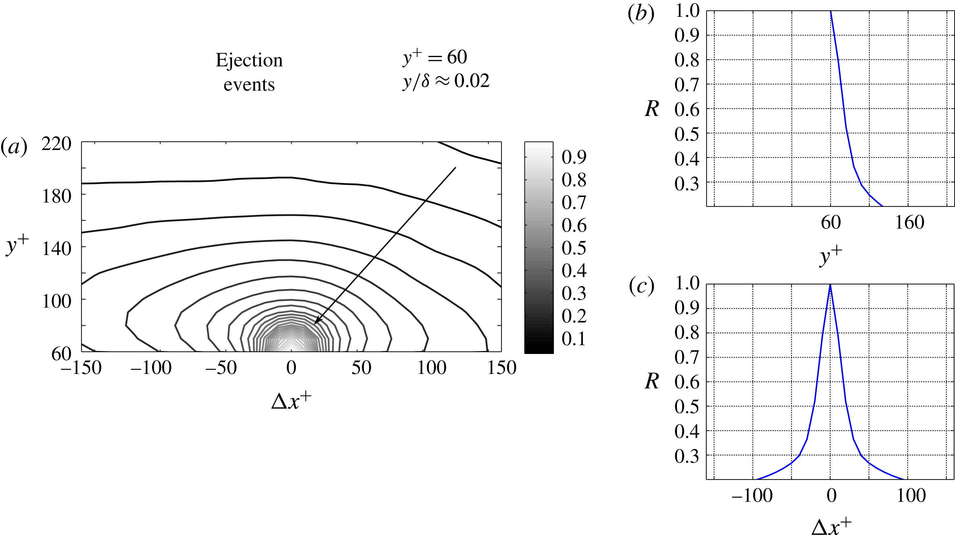
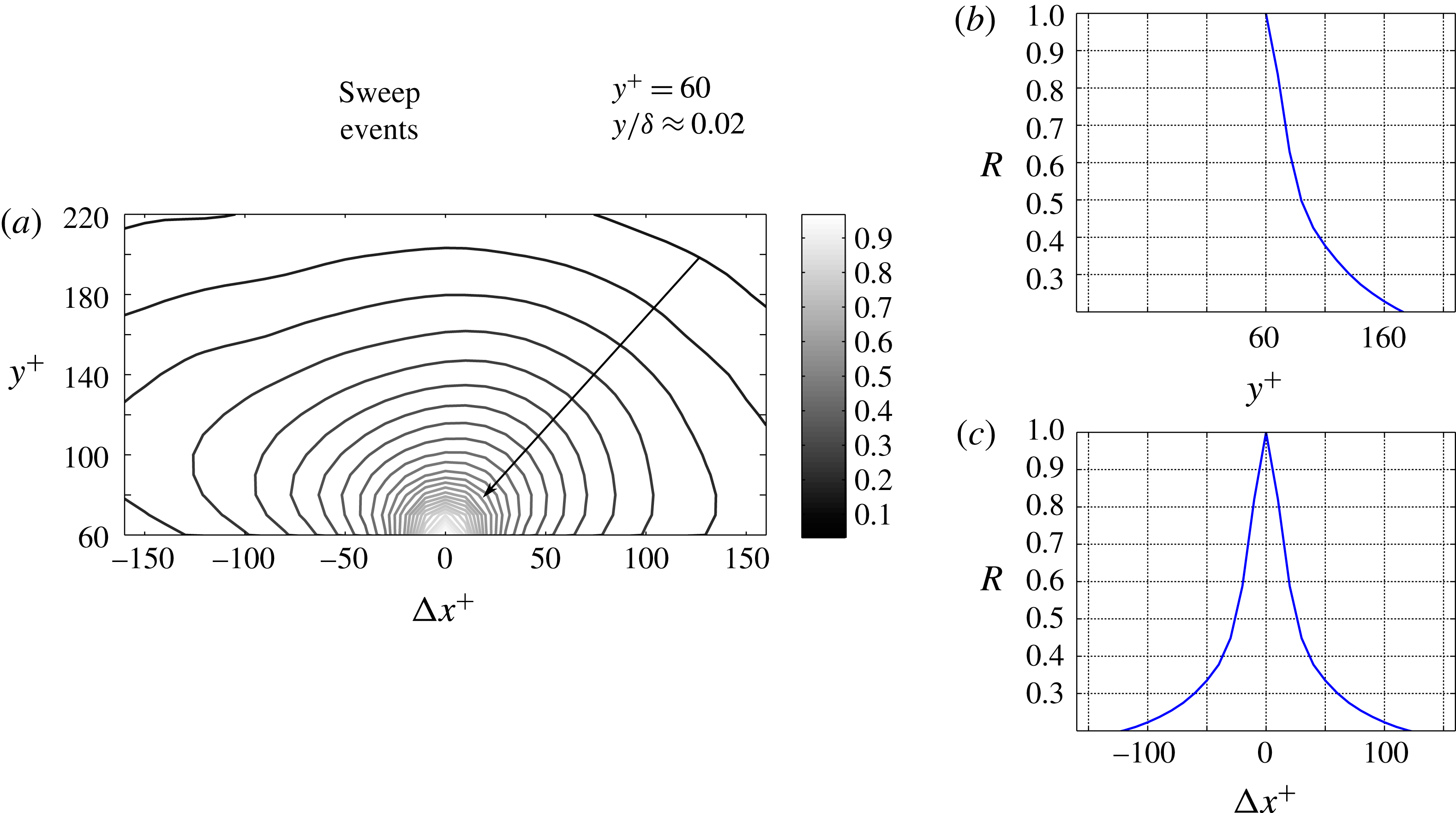
. Even if the shape of the autocorrelation maps is similar for both ejection and sweep events, the autocorrelation coefficients of ejection events decay to zero for shorter shifts than those of sweep events. This can be also observed in figures 13(b) and 13(c), and in figures 14(b) and 14(c), where sections of the autocorrelation coefficients maps along the wall-normal and streamwise directions through the origin are shown.
Autocorrelation coefficient map of ejection events, at
 $y^{+}=60$
(a). Sections along the wall-normal (b) and streamwise (c) directions of the autocorrelation coefficients map as presented in (a).

Autocorrelation coefficient map of sweep events, at
 $y^{+}=60$
(a). Sections along the wall-normal (b) and streamwise (c) directions of the autocorrelation coefficients map as presented in (a).

From these profiles, we can quantify the size of both ejection and sweep events, at
 $y^{+}=60$
. If
 $R=0.5$
is chosen as threshold, the characteristic streamwise extent of ejection events at
 $y^{+}=60$
is approximately
 $40$
wall units (figure 13
c), whereas the characteristic streamwise extent of sweep events at
 $y^{+}=60$
is approximately
 $60$
wall units (figure 14
c). Therefore, at
 $y^{+}=60$
, sweep events are approximately 50 % larger in the streamwise extent than ejection events. Note that even at this high threshold, the difference is better than our spatial resolution of the measurements (the vector spacing is 10 wall units while the window size is 20 wall units). If we relaxed this threshold to a lower value, the difference in size would be even more discernible. However, in order to remain consistent with previous studies, the threshold value of 0.5 is chosen. From figures 13(b) and 14(b), the wall-normal extent of
 $Q^{-}$
events is similar to their streamwise extent. In consequence of this, the structure of sweep events is around 50 % larger in size than the structure of ejection events. This agrees with the analysis of the spectra (figure 11), where at high wavenumbers (short wavelengths) the spectral content of the ejection events increases with respect to the spectral content of the sweep events, while the opposite can be observed at low wavenumbers.
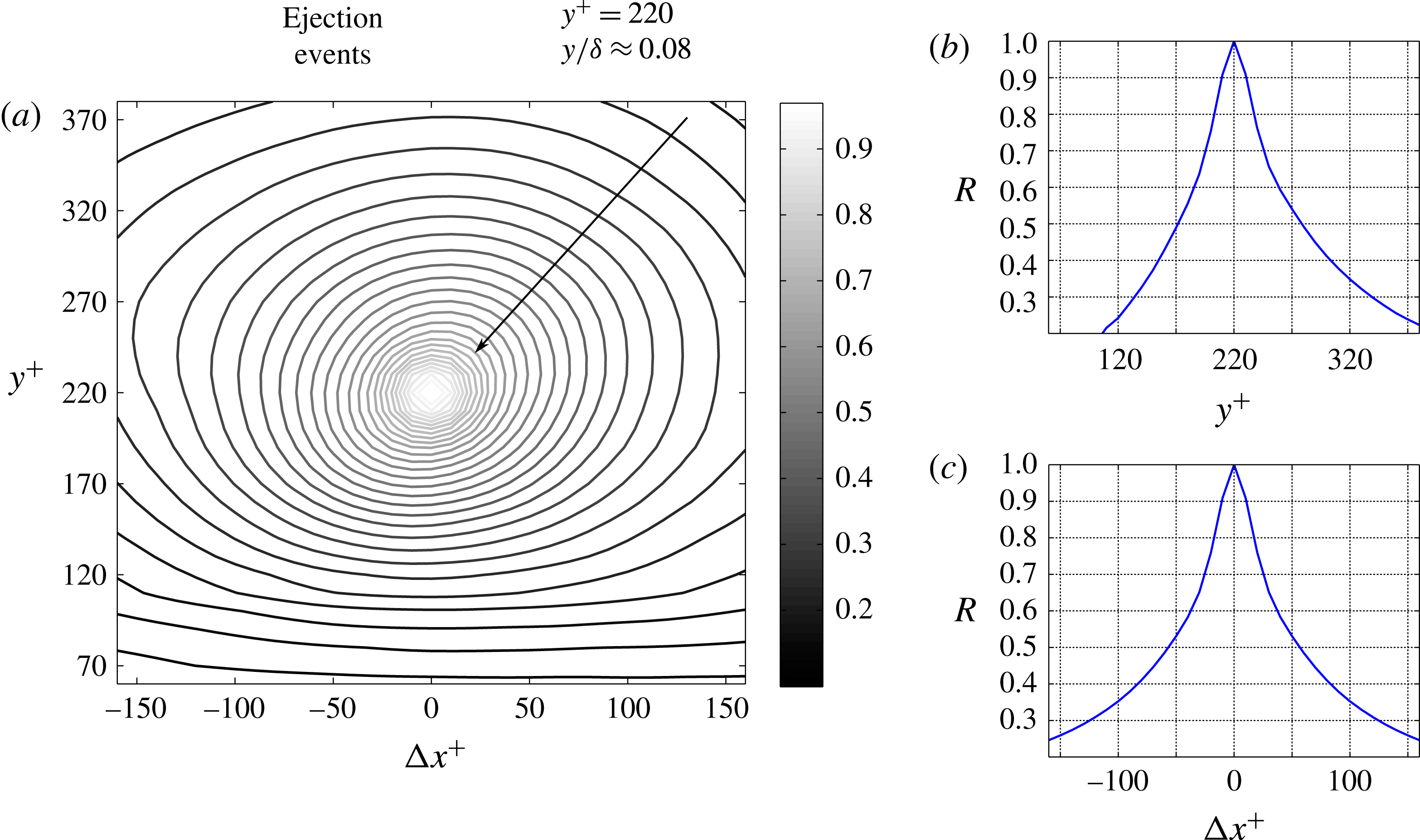
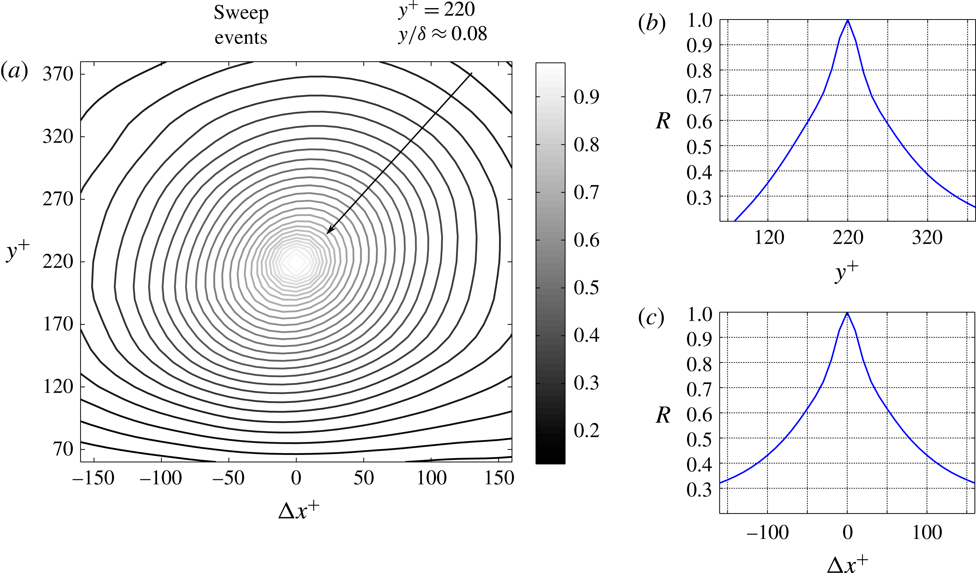
Farther from the wall, at
 $y^{+}=220$
, the structure of ejection and sweep events appears more circular, as can be observed in figures 15 and 16. Lin et al. (Reference Lin, McWilliams, Moeng and Sullivan1996) reported a similar finding from LES of the planetary boundary layer, where conditional sampling was used to characterize the spatial structure of
 $Q^{-}$
events. They noticed that in proximity to the wall, ejection and sweep events exhibit an elongated (or ‘streaky’) shape, while farther from the wall the structure of the
 $Q^{-}$
events becomes progressively circular.
The size of
 $Q^{-}$
events can be assessed based on the profiles along the wall-normal and streamwise directions of the autocorrelation coefficients maps, which are presented in figures 15(b) and 15(c), for ejection events, and in figures 16(b) and 16(c), for sweep events. As it can be seen, the extent of ejection events along wall-normal and streamwise directions is approximately 110 and 115 wall units (figures 15
b and 15
c respectively), while the extent of sweep events along wall-normal and streamwise directions are approximately 140 and 135 wall units (figures 16
b and 16
c, respectively). If a threshold of
 $R=0.5$
is chosen in the autocorrelation coefficients maps, the extent of both ejection and sweep events can be extended to the range of wall distances
 $60<y^{+}<1050$
(figure 17). Overall, the structure size of sweep events is larger than the structure size of ejection events. At wall-normal distances
 $y^{+}<450$
, the wall-normal extent of both
 $Q^{-}$
events is almost equivalent to its respective streamwise counterpart. On the other hand, at wall-normal distances larger than
 $y^{+}=450$
, the wall-normal extent of the event structure is larger than their respective streamwise extent.
Autocorrelation coefficient map of ejection events, at
 $y^{+}=220$
(a). Sections along the wall-normal (b) and streamwise (c) directions of the autocorrelation coefficients map as presented in (a).

These observations on the size of ejection and sweep events are consistent with the spectra presented in figure 11. When examining the spectra related to sweep events, a larger spectral contribution is contained at low wavenumbers in comparison to the spectra related to ejection events, at a given wall-normal distance. In figure 11, the darkest stripe marking the largest spectral content has a larger extension for sweep events than for ejection events.
Autocorrelation coefficient map of sweep events, at
 $y^{+}=220$
(a). Sections along the wall-normal (b) and streamwise (c) directions of the autocorrelation coefficients map as presented in (a).

Over the whole range of wall-normal locations, the size of both ejection and sweep events increases monotonically. Two linear trends could be identified in figures 17(a) and 17(b), and marked with lines of different colours. The first linear trend characterizing the size of the ejections covers the range
 $y^{+}<450$
. At
 $y^{+}>450$
, the ejections increase in size with the wall distance, by following a lower slope than in the range
 $y^{+}<450$
. An analogous change in the slope occurs also to the size of the sweeps, even if this takes place at
 $y^{+}\approx 400$
, and therefore at a lower wall-normal location. As already observed in the previous section, this change in the slope can be explained as a transition from a range of wall-normal locations where the wall-attached events are dominant, to a range in which the wall-detached events are prevalent.
Characteristic extent of ejection (a) and sweep events (b) along the streamwise (empty circles, ○) and wall-normal (filled squares, ▪) directions, at different wall-normal distances. Results are based on autocorrelation coefficients maps, and
 $R=0.5$
was chosen as a threshold. In the insets, the same data are reported on log–log plots, and exponential fitting laws are estimated.

It is worth noting that while the first range of the trend exhibits a similar slope for both ejections and sweeps, the second range presents different behaviours when comparing the two types of
 $Q^{-}$
events. In particular, at
 $y^{+}>450$
, the linear trend relative to the ejections is characterized by a larger slope than the linear trend relative to the sweeps. This suggests that at wall-normal locations
 $y^{+}>450$
, the dominance of the wall-detached events over the wall-attached ones is stronger for sweeps than for ejections. In other words, the probabilities of finding wall-detached objects is higher for sweep than for ejection events. This observation is consistent with the quantification of Lozano-Durán et al. (Reference Lozano-Durán, Flores and Jiménez2012), presented in table 2 of their paper. According to their analysis in a DNS channel flow, the numerical fraction of wall-attached ejections is larger than the numerical fraction of wall-attached sweeps. Specifically, they found that the wall-attached ejections are approximately 45 % of the whole number of ejections, and the wall-attached sweeps are approximately 39 % of the whole number of sweeps.
In the insets of figure 17, the extent of ejections (a) and sweeps (b) along the wall-normal and streamwise directions are given in a log–log plot. Exponential fitting laws associated with the relationships between sizes and wall distances are also given. At increasing wall-normal locations, ejection events increase in size more rapidly than sweep events. The trend slope relative to the ejection size is higher (larger exponent) than the trend slope relative to the sweep size (smaller exponent), while the trend slope relative to all the RSS is intermediate between these two. Nonetheless, a modest discrepancy is observed between the exponents of the three scaling laws.
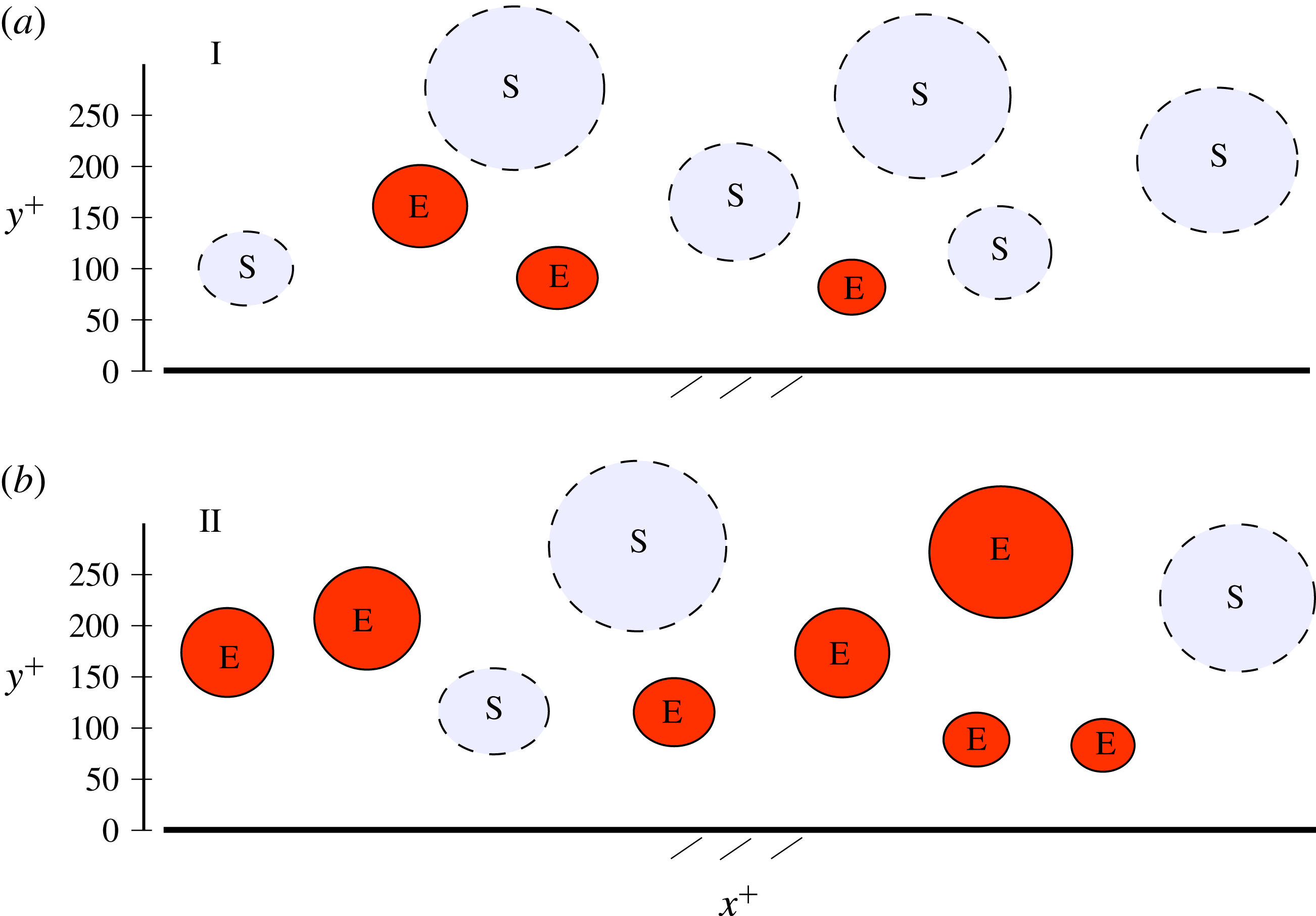
An important piece of evidence from the autocorrelation coefficients maps shown in figures 13–16, and confirmed from the analysis presented in figure 17, is that the ejection events are smaller than the sweep events. This difference in size is particularly large in proximity to the wall, and it could be explained by the spatial organization of ejection and sweep events within the TBL, also in relation to the hairpin vortices. The intense ejection events are typically located in between the legs of hairpin packets, as observed by various investigators (Zhou et al. Reference Zhou, Adrian and Balachandar1996; Adrian Reference Adrian2007, and Jodai & Elsinga Reference Jodai and Elsinga2016, among others). On the other hand, sweep events tend to be associated with the downwash of fluid produced by the hairpin vortices, externally with respect to the hairpin packets. Therefore, ejection events are preferentially located within hairpin packets, while sweep events tend to be found in the space between two spanwise adjacent hairpin packets. It descends that the spatial extension of each ejection event related to a hairpin vortex is limited in the spanwise and wall-normal directions by the hairpin size, and in the streamwise direction by the downwash fluid induced by the head of the following hairpin, part of the packet. By contrast, sweep events can spatially develop over larger extensions, as they are located externally to the hairpin packets, and each leg of the hairpin vortices constituting each individual packet contributes to their formation.
However, it is worth stressing that the described difference in the sizes of ejections and sweeps was not observed in the DNS simulations of a channel flow by Lozano-Durán et al. (Reference Lozano-Durán, Flores and Jiménez2012) and Lozano-Durán & Jiménez (Reference Lozano-Durán and Jiménez2014). It transpires that an equally valid and plausible explanation for the observed difference in size can be found in the entrainment of quiescent fluid, which occurs in TBLs, but not in channel flows. However, it is complicated to come up with a definitive explanation in support of the experimental evidence that sweep events are statistically larger than ejection events in TBLs, and further investigations are necessary to shed more light on this issue.
4.3 Intense
$Q^{-}$
events and their time evolution

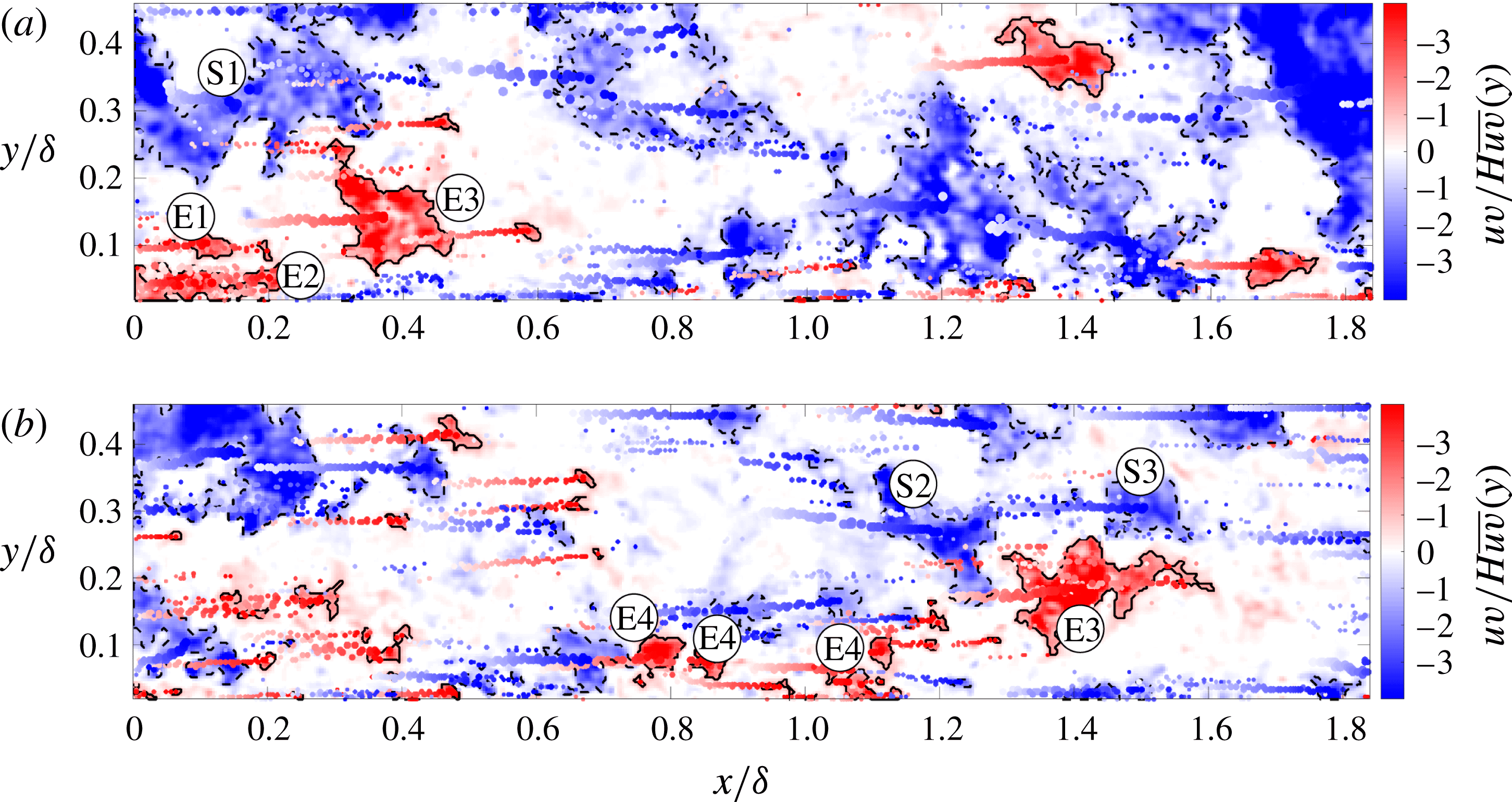
In figure 18, two snapshots at two instants of
 $Q^{-}$
events are presented. Panel (a) is a snapshot taken at the same instant as the snapshot given in figure 2, where both positive and negative quadrant events are shown. The time delay between the snapshots is
 $\unicode[STIX]{x0394}t=1.33\unicode[STIX]{x1D6FF}/U_{\infty }$
. The shades of red (ejection events) and blue (sweep events) indicate the intensity of the non-dimensional negative quadrant RSS. Regions delimited by black continuous lines mark intense ejection events, while black dashed lines are used to mark intense sweep events, both identified with the criterion of (2.1) (
 $H=1.8$
). In addition, spots of different sizes and shades mark the time development of the weighted centroids of the intense events. Specifically, the size of each spot is proportional to the extension of the related event, while its shade reflects the time span at which a given weighted centroid has been detected. In panel (a), tags were added to the most significant events, in order to identify these same events in panel (b).
Snapshots of negative quadrant events of the RSS, at two different time instants with
 $\unicode[STIX]{x0394}t=1.33\unicode[STIX]{x1D6FF}/U_{\infty }$
. Black continuous lines mark intense ejection events, while black dashed lines mark intense sweep events, both identified with the criterion shown in (2.1). Spots of different sizes and shades mark the time evolution of the weighted centroids of the intense events. The most significant events are tagged, with the aim of identifying the same events in the two snapshots.

The complete time evolution of the
 $Q^{-}$
events presented in figure 18 can be observed in supplementary movie 2. This movie shows the time evolution of the same
 $Q^{-}$
events presented in movie 1, even though the
 $Q^{-}$
events are here distinguished into ejection and sweep events. The time span covered in this movie is
 $1.33\unicode[STIX]{x1D6FF}/U_{\infty }$
, therefore the movie reduces the flow velocity of approximately 150 times. As we can observe, the large sweep event S1 gives birth to the two smaller sweep events S2 and S3. During the time span of
 $1.33\unicode[STIX]{x1D6FF}/U_{\infty }$
, the events originating from S1, S2 and S3, are located closer to the wall than S1 itself. This can be appreciated from the position of the weighted centroids of the three events, S1, S2 and S3.
Moreover, after its separation from S1, S3 moves at a larger advection velocity than S2, and it travels a larger streamwise distance in the same time span. Also, if we focus on ejection events, E1 disappears in the time span that separates the two snapshots, while E2 gives birth to several smaller events, three of which were tagged as E4 in the bottom snapshot of figure 18. Events E4 are also located farther from the wall than the ejection event E2 originating them, evidence that they have moved upwards. Analogous observation can be made for the ejection event E3, which moves towards a higher wall-normal location even if it does not give birth to any additional ejection events. Another observation is that the advection velocity of E3 is clearly lower than S2 and S3. This is consistent with E3 being closer to the wall than S2 and S3. Similar considerations apply to E4.
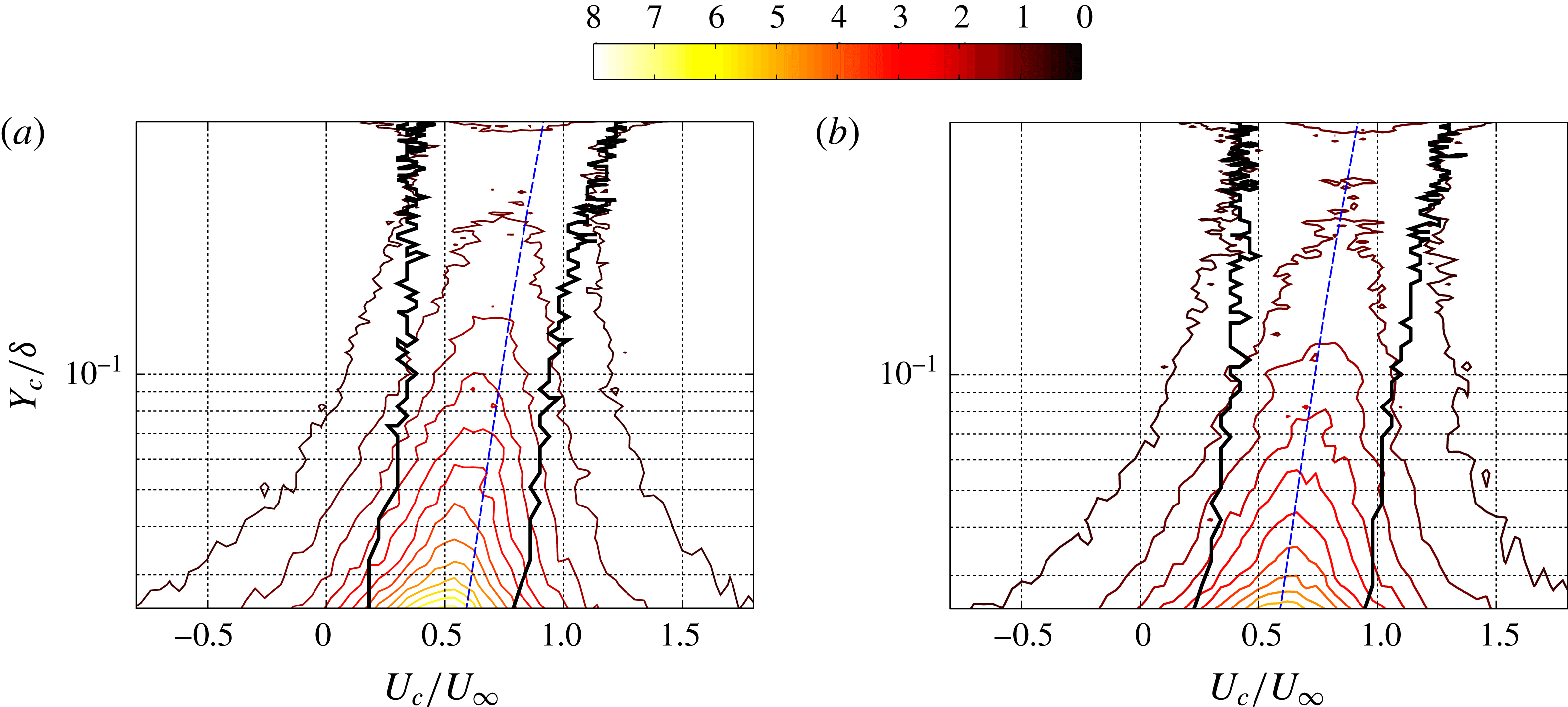
Joint probability density functions between the streamwise component of the local velocities (
 $U_{c}$
) of the intense ejection (a) and sweep (b) events, and their wall-normal locations (
 $Y_{c}$
). The black thicker line is a contour of the 50 % of the peak value at each wall-normal location. The blue dashed line represents the average streamwise velocity of the flow.

The analysis of figure 18 enabled us to document the time evolution of only one sweep event and three ejection events. In the following, sweep and ejection events are identified throughout the whole dataset with the criterion of (2.1), and tracked in time, with the aim of statistically quantifying their (i) local velocities, (ii) wall-normal locations, (iii) intensities, and (iv) size. The first part of the analysis focuses on the local convection velocities of the tracked
 $Q^{-}$
events. The investigation is based on the forward–backward tracking of
 $1.82\times 10^{6}$
ejection events and
 $1.65\times 10^{6}$
sweep events (§ 2.1), and therefore on the same number of local velocities. The quantification of the displacement of each tracked event among two different PIV snapshots is calculated in relation to the positions of the weighted centroids of the events, at the two different time instants.
It is worth noting that, in consequence of splitting of events across time, one event at a certain time instant can be associated with two or more events at the following time instant, thus leading to two or more local velocities. On this respect, all the local velocities obtained from time tracking intense transport events contributed to the statistics presented in the following. Furthermore, the wall-normal location associated with a certain displacement (and thus local velocity) is the wall-normal location of the weighted centroid of the forward tracked intense event, by convention.
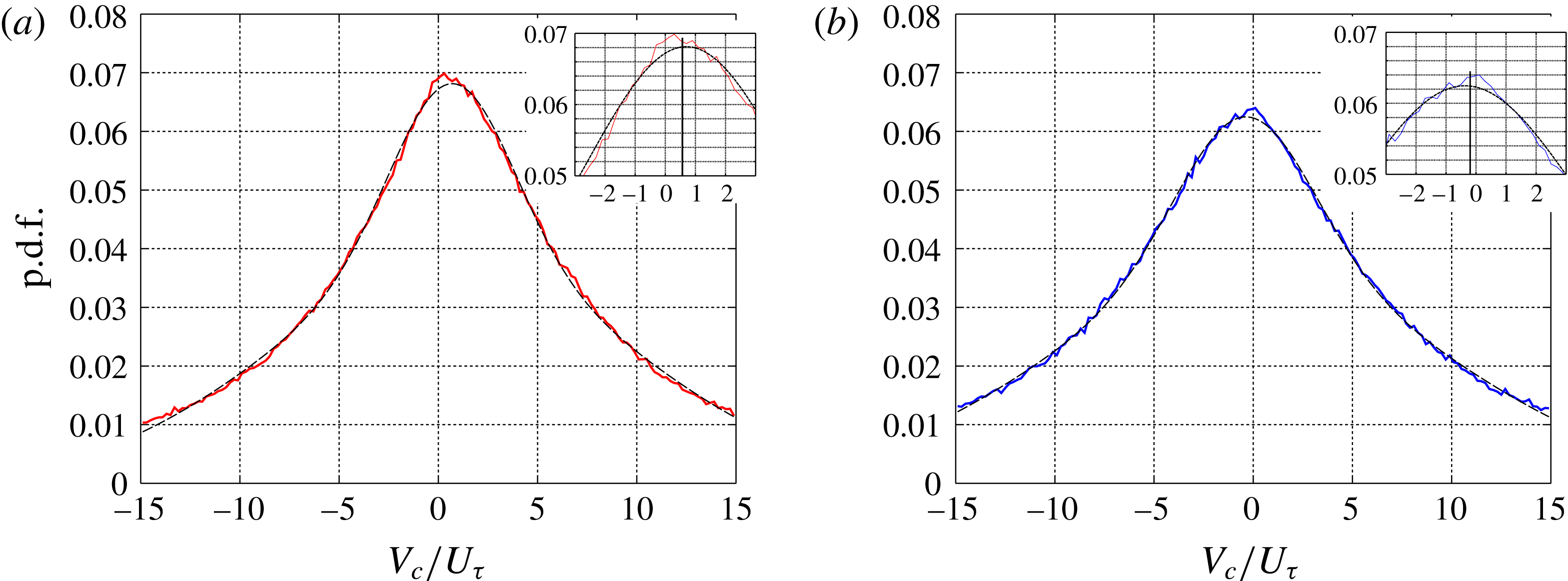
Probability density functions of the wall-normal component of the local velocities (
 $V_{c}$
) of the intense ejection (a) and sweep (b) events (continuous line), and a two-term Gaussian fitting curve (dashed line). The vertical lines in the insets represent the average values, which are respectively
 $0.56\pm 0.01$
for the ejection events and
 $-0.2\pm 0.01$
for the sweep events.

In figure 19, the joint probability density functions between the streamwise component of the local velocities (
 $U_{c}$
) of ejections and sweeps, and their wall-normal locations is presented. In addition to this, two black thick lines identify a region where the number of samples of
 $U_{c}$
is larger than 50 % of the largest number of samples at a given wall-normal location, and the blue dashed line represents the average streamwise velocity of the flow. The two plots appear very similar, and it seems that one plot is obtained by horizontally shifting the others. As expected, the ejection events are characterized by statistically lower streamwise local velocities than the sweep events. These features are consistent with the estimate of the characteristic wave velocities based on power spectra and presented in figure 12. In proximity to the wall, the ejection events are characterized by a larger distribution of
 $U_{c}$
than the sweep events, while at increasing distances from the wall this difference tends to disappear. This is again consistent with the finding from the analysis of the spectra in figure 11. However, the extension of the region of each plot identifying 50 % of the peak value at a given wall-normal location (black thick lines, figure 19) suggests that the streamwise local velocities of the ejection events decay more rapidly from their peak values than the streamwise local velocities of the sweep events. This feature can be observed everywhere in the flow, even if it is more significant closer to the wall. This can be attributed to the larger size of the sweep events, that might produce larger changes in the position of the weighted centroid at adjacent time instants. Moreover, larger absolute values of
 $U_{c}$
lead to larger absolute deviations for a given percentage deviation. At
 $Y_{c}/\unicode[STIX]{x1D6FF}<0.4$
, the probability of detecting a centroid of an intense
 $Q^{-}$
event diminishes for increasing distances from the wall. The range of streamwise local velocities becomes also increasingly more narrow for growing wall distances.
In figure 20, the probability density functions of the wall-normal component of the local velocities (
 $V_{c}$
) of ejections and sweeps is given. A two-term Gaussian fit is included to each plot, drawn with a dashed line. The very large positive and negative values of wall-normal velocity, which have been obtained and reported in the p.d.f.s, are probably an artefact of the tracking method. They could be attributed to the finite size of the field of view, and to splitting and merging of events. However, these sources of bias tend to compensate each other when calculating the average value. This can be inferred by the symmetry in the distribution of the p.d.f.s around the mode value, which makes the mode value approximately match the average value. The peak values of each fitting curve are
 $V_{c}/U_{\unicode[STIX]{x1D70F}}=0.65$
for ejection events and
 $V_{c}/U_{\unicode[STIX]{x1D70F}}=-0.30$
for sweep events. Similar values are obtained when the average is calculated from the range
 $-15<V_{c}/U_{\unicode[STIX]{x1D70F}}<15$
. These values are
 $V_{c}/U_{\unicode[STIX]{x1D70F}}=0.56\pm 0.01$
for ejection events and
 $V_{c}/U_{\unicode[STIX]{x1D70F}}=-0.20\pm 0.01$
for sweep events. As expected, ejection events have a preferential tendency towards moving upwards (positive average velocity), and therefore away from the wall, while sweep events tend to move downwards (negative average velocity). However, the wall-normal local velocities of the ejection events is approximately double than the wall-normal local velocities of the sweep events, and they are both a fraction of the friction velocity of the turbulent boundary layer,
 $U_{\unicode[STIX]{x1D70F}}$
.
The above result is different from the observations of Lozano-Durán & Jiménez (Reference Lozano-Durán and Jiménez2014), who found peaks in the p.d.f.s of the vertical advection velocities at
 $V_{c}=U_{\unicode[STIX]{x1D70F}}$
and at
 $V_{c}=-U_{\unicode[STIX]{x1D70F}}$
, respectively for ejection and sweep events. Several reasons could explain this discrepancy. Firstly, the flow investigated in Lozano-Durán & Jiménez (Reference Lozano-Durán and Jiménez2014) is a channel, while the present study investigates a TBL, meaning that a different flow could motivate different characteristics of the momentum transport. Secondly, Lozano-Durán & Jiménez (Reference Lozano-Durán and Jiménez2014) analysed the full domain contained within the two walls of the channel flow, whereas the present study examines only half of the wall-normal TBL extent, namely the range
 $50<y^{+}<1280$
(
 $0.02<y/\unicode[STIX]{x1D6FF}<0.5$
). Moreover, the present analysis is limited to a two-dimensional domain, where the estimated location of the weighted centroid of an intense event might deviate from its actual physical location, in lieu of its three-dimensional extension. However, statistically this difference would be minimal given the number of events that contribute to the measurement.
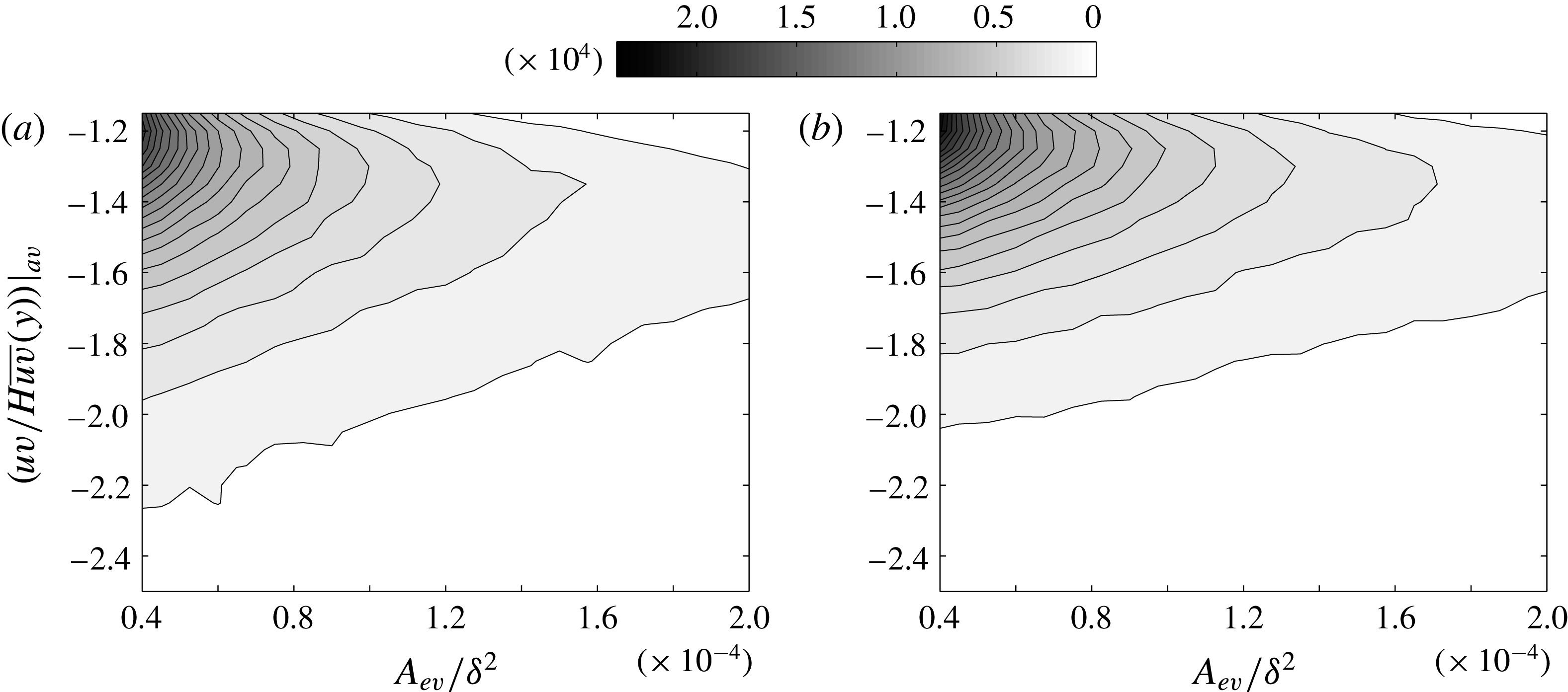
After the statistical analysis of the local velocities of the
 $Q^{-}$
events, the relationship between intensity and area, and intensity and wall-normal position is examined. A characteristic area of the intense events (
 $A_{ev}$
) is obtained by multiplying the number of points constituting these events by the square of the vector spacing. The characteristic area of the intense events is then non-dimensionalized by the square of the boundary layer thickness (
 $\unicode[STIX]{x1D6FF}^{2}$
). The intensity of the
 $Q^{-}$
events is non-dimensionalized by the local average RSS multiplied by the coefficient
 $H$
, which is the threshold quantity used to identify these intense events. In figure 21, the joint probability density functions between the intensity and the area of intense ejections (a) and sweeps (b) are presented. Statistics are based on
 $1.83\times 10^{6}$
ejection events and
 $1.67\times 10^{6}$
sweep events. Both the j.p.d.f.s are characterized by a strong peak for small areas and low intensities (top left of the chart). This is evidence for the predominance of the small-sized and low-intensity events. A common feature to both the j.p.d.f.s is that the very intense events (say non-dimensional intensities lower than
 $-1.8$
) tend to diminish in number for increasing size.
Joint probability density functions between the areas of the intense ejection (a) and sweep (b) events and their intensities averaged over the respective areas.

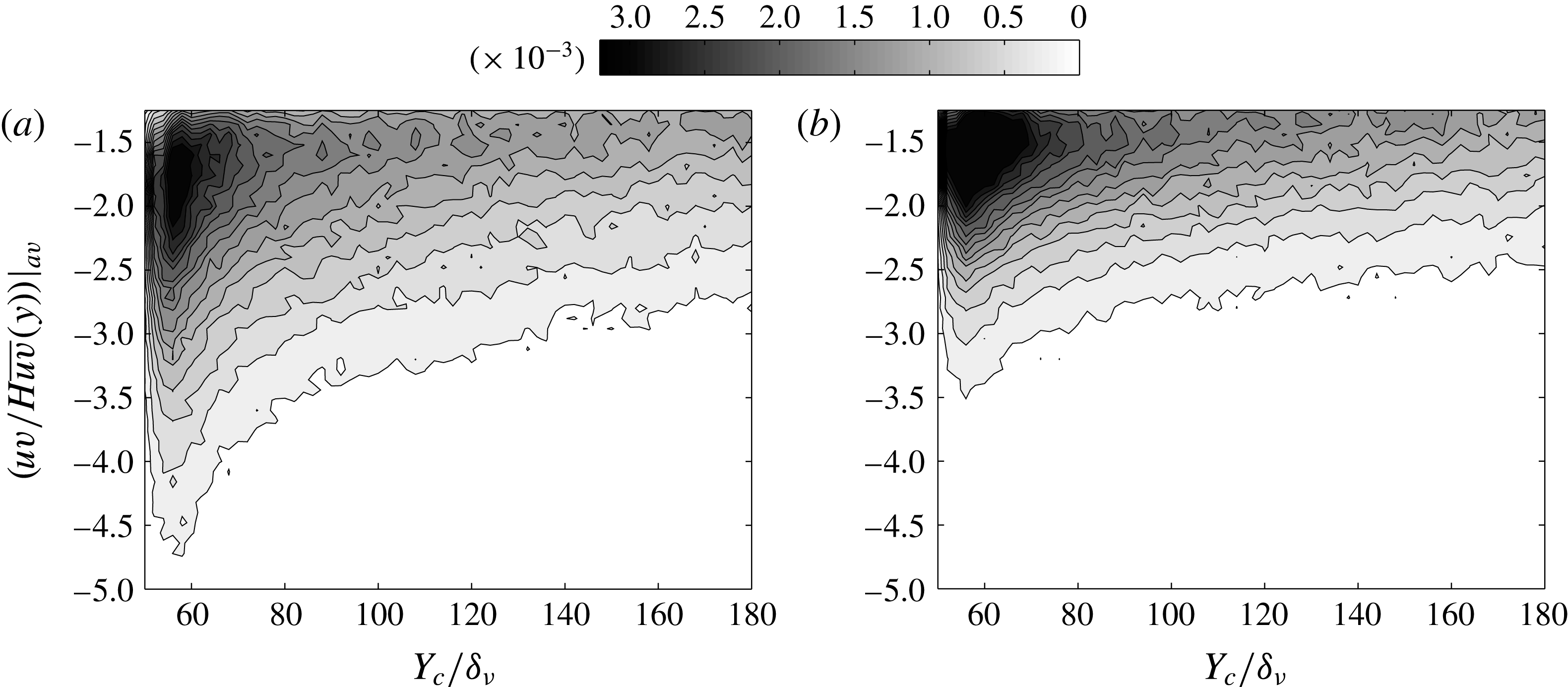
Joint probability density functions between the wall-normal locations of the intense ejection (a) and sweep (b) events and their intensities averaged over the respective areas.

On the other hand, the events characterized by low intensity tend to be less probable for growing size. Negative quadrant events with larger areas have smaller ranges of intensities. Overall, the ejection events are characterized by smaller sizes and higher intensities than the sweep events. The larger area of the sweep events observed in figure 21 and based on tracking is consistent with the finding obtained from autocorrelation functions (figures 13–17). Therefore, the slightly larger contribution of the ejection events to the RSS can be attributed to a larger number of events of smaller size and higher intensity.
The preferential wall-normal location of ejection and sweep events in relation to their intensity can be quantified from the j.p.d.f.s presented in figure 22. The non-dimensional wall-normal location of the weighted centroids of the
 $Q^{-}$
events is given by
 $Y_{c}/\unicode[STIX]{x1D6FF}_{\unicode[STIX]{x1D708}}$
, where
 $\unicode[STIX]{x1D6FF}_{\unicode[STIX]{x1D708}}$
is the viscous length scale
 $\unicode[STIX]{x1D6FF}_{\unicode[STIX]{x1D708}}=\unicode[STIX]{x1D708}/U_{\unicode[STIX]{x1D70F}}$
. The two j.p.d.f.s reveal that the
 $Q^{-}$
events tend to be most probably found in proximity to the wall (
 $60<y^{+}<80$
), where also high-intensity events have more chance to be detected. If we distinguish between ejection and sweep events, we can observe that the ejection events detected at the wall are characterized by higher intensities than the near-wall sweep events. The intense sweep events are therefore more homogeneous in intensity. This means that a larger number of sweep events falls within shorter ranges of intensity, and that the curves of equal probability in the j.p.d.f. are closer to each other in vertical direction, in figure 22(b). At wall-normal locations higher than
 $y^{+}=130$
, the two j.p.d.f.s do not change significantly and the dependence of the results on wall-normal location is modest.
4.4 Number density of the intense
$Q^{-}$
events

In the previous subsections, the
 $Q^{-}$
events have been analysed as two distinct entities. Here, the statistical presence of intense
 $Q^{-}$
events in the neighbourhood of an intense ejection or sweep event is examined. Specifically, we intend to estimate the number density of intense sweep events in the vicinity of an intense ejection event
 $D_{e\rightarrow s}$
, and vice versa
 $D_{s\rightarrow e}$
.
Number density of (a,c,e) the intense sweep events in the neighbourhood of an intense ejection event,
 $D_{e\rightarrow s}$
, and of (b,d,f) the intense ejection events in the neighbourhood of an intense sweep event,
 $D_{s\rightarrow e}$
, at three different wall-normal positions (
 $y^{+}=60$
,
 $y^{+}=140$
, and
 $y^{+}=220$
).

To achieve this, a procedure was established as follows: each point of the
 $uv$
frames associated with an intense ejection event was identified and marked with the value one, while all the remaining points were set to zero. The same procedure was applied for the intense sweep events. The obtained frames containing markers of the ejection events were cross-correlated with the corresponding frames containing markers of the sweep events, at different distances from the wall. The result of this analysis is presented in figure 23, for three wall-normal locations, namely at
 $y^{+}=60$
(
 $y/\unicode[STIX]{x1D6FF}\approx 0.02$
),
 $y^{+}=140$
(
 $y/\unicode[STIX]{x1D6FF}\approx 0.04$
), and
 $y^{+}=220$
(
 $y/\unicode[STIX]{x1D6FF}\approx 0.08$
).
These correlation maps show that for a given wall-normal position, the general probability to find intense sweep events in the vicinity of an intense ejection event is larger than the probability to detect intense ejection events in the neighbourhood of an intense sweep event. In other words, ejection events have more chance to be surrounded by
 $Q^{-}$
events of opposite nature than sweep events. Furthermore, the ejection events in the neighbourhood of a sweep event are preferentially located below it, and therefore closer to the wall, while the sweep events tend to be positioned more uniformly all around an ejection event, with a weak prevalence for higher wall-normal locations. It is also worth noting that at a given wall distance, the extension of the lowest intensity level in the contour map is affected by the size of the intense
 $Q^{-}$
events themselves.
The ejection events tend to be smaller in size than the sweep events, consistent with the autocorrelation maps presented in the previous subsections (figures 13–16). Number densities at wall-normal positions higher than
 $y^{+}=220$
have not been reported in figure 23, because both the larger size of the
 $Q^{-}$
events and the lower probability of finding
 $Q^{-}$
events of different nature result in a very large extension of the low-intensity levels in the contour map. They were therefore omitted because they are not very meaningful for the discussion.
Number density dominance of (a,c,e) the intense ejections versus intense sweeps in the neighbourhood of an intense ejection event,
 $D_{e\rightarrow Q^{-}}$
, and of (b,d,f) the intense sweeps versus intense ejections in the neighbourhood of an intense sweep event,
 $D_{s\rightarrow Q^{-}}$
, at three different wall-normal positions (
 $y^{+}=60$
,
 $y^{+}=140$
, and
 $y^{+}=220$
).

In order to know whether an intense
 $Q^{-}$
event tends to be surrounded by intense
 $Q^{-}$
events of the same nature or of the opposite nature, a procedure analogous to the one described above was established. The positions of the intense
 $Q^{-}$
events were identified in the
 $uv$
frames, and marked for ejection events
 $(+1)$
and for sweep events
 $(-1)$
, while all the remaining points of the frame were set to zero. In a similar way, we created frames identifying the positions of the intense ejection events, and frames identifying positions of the intense sweep events. The frames containing the positions of the intense ejection events were one-dimensionally correlated with frames containing both ejection and sweep events markers, which identify the positions of all the intense
 $Q^{-}$
events.
The same operation was done for the frames containing the positions of the intense sweep events. In this way, we could obtain an estimate for the number density dominance of the intense ejection versus sweep events in the vicinity of an intense ejection event,
 $D_{e\rightarrow Q^{-}}$
, and of an intense sweep event,
 $D_{s\rightarrow Q^{-}}$
. Figure 24 shows the outcome of this analysis. Positive values were obtained everywhere in the maps, and also for
 $|\unicode[STIX]{x0394}x^{+}|>150$
, even if this range is not presented in figure 24. This indicates that the intense
 $Q^{-}$
events are preferentially surrounded by intense
 $Q^{-}$
events of the same nature, i.e. ejection events tend to be found in the vicinity of an ejection event, and sweep events tend to be found in the vicinity of a sweep event. Lozano-Durán et al. (Reference Lozano-Durán, Flores and Jiménez2012) noticed a similar spatial organization in a channel flow. They observed that objects of different kind tend to align spanwise rather than streamwise. Unfortunately, the dataset in our possession does not enable us to examine the spatial organization of ejections and sweeps in the spanwise direction.
Conceptual sketch of spatial organization, size, and shape of intense ejection and sweep events, at a range of wall-normal locations
 $50<y^{+}<300$
. Two scenarios are statistically more probable: (I), prevalence of intense sweep events (a); (II), prevalence of intense ejection events (b).

In addition, the decay of the number density dominance is more rapid for ejection events than for sweep events. This can be attributed to both a lower number of intense events of the same nature and a larger number of intense events of the opposite nature. The latter explanation is confirmed from figure 23, where we observed that ejection events are more preferentially surrounded by
 $Q^{-}$
events of opposite nature than sweep events. The observed faster decay in the
 $D_{e\rightarrow Q^{-}}$
map is progressively less evident for increasing distances from the wall. At
 $y^{+}=200$
, the two number density maps are more similar than at lower wall-normal locations. The isocontours of
 $D_{e\rightarrow Q^{-}}$
are characterized by a larger extension than the isocontours of
 $D_{s\rightarrow Q^{-}}$
.
Based on statistical evidence presented in this section it is possible to draw a conceptual sketch summerizing spatial organization, shapes and size of the intense
 $Q^{-}$
events, at the range of wall-normal location
 $50<y^{+}<300$
. This sketch is given in figure 25. From the conclusion obtained from analysis of the number density dominance (figure 24), the same kinds of events can be found in the neighbourhood of a
 $Q^{-}$
event. Therefore, two possible scenarios can be identified: (I) a scenario where sweep events are dominant (figure 25
a), (II) a scenario where ejection events are dominant (figure 25
b).
At a given wall distance, ejections are characterized by a smaller size than sweeps, and the size of both ejections and sweeps increases linearly with the wall-normal location, in the range
 $50<y^{+}<300$
. The size of the
 $Q^{-}$
events depicted in figure 25 follows the estimation reported in figure 17. Also, their shape is elongated in the streamwise direction in proximity to the wall, while, when moving towards the outer region, they tend to be more round, as we learnt from the autocorrelation maps presented in figures 13–16. From the number density maps reported in figure 23, ejection events in the neighbourhood of a sweep event tend to be located upstream and closer to the wall. On the other hand, sweep events surrounding an ejection event tend to be more uniformly distributed around it. The spatial organization of
 $Q^{-}$
events obtained from statistical considerations and presented in figure 25 is also supported by instantaneous snapshots, as can be seen in figure 18, and in supplementary movie 2.
5 Conclusion
In the present work, the transport of momentum was investigated using time-resolved planar PIV data of a turbulent boundary layer at the Reynolds number of
 $(Re_{\unicode[STIX]{x1D70F}}=)2700$
, in the range of wall-normal locations from
 $50y^{+}$
to
 $1280y^{+}$
(which is equivalent to
 $0.46\unicode[STIX]{x1D6FF}$
).
The RSS contributions were classified based on the quadrant analysis introduced by Wallace et al. (Reference Wallace, Eckelman and Brodkey1972). The
 $Q^{-}$
events account for 150 % of the total RSS, and the
 $Q^{+}$
events account for only
 $-50\,\%$
of the total RSS. Furthermore, the intense RSS events were identified with a criterion analogous to Willmarth & Lu (Reference Willmarth and Lu1972), where the absolute value of the local Reynolds stress
 $|uv(x,y)|$
has to be larger than the Reynolds stress averaged over the streamwise direction
 $|\overline{uv}(y)|$
multiplied by a constant
 $H=1.8$
. It was found that the percentage contribution of the intense
 $Q^{-}$
events to the total negative quadrant RSS accounts for more than 80 %, while the average of their total area is lower than 30 % of the whole extension of the measurement plane. This is evidence that the distribution of the RSS in the near-wall region of the turbulent boundary layer is strongly inhomogeneous and intermittent. The contribution of ejections and sweeps to the negative RSS was also assessed. It was found that 53 % of the negative RSS comes from ejection events, while 47 % of the negative RSS is obtained from sweep events.
The spectral content of the RSS fluctuations was quantified at different wall-normal locations. It was observed that the RSS fluctuations exhibit the largest range of time and length scales in proximity to the wall, while RSS events of longer time and length scales tend to be increasingly more energetic at growing wall-normal locations. From the wavenumber–frequency power spectral density of the RSS fluctuations, we could see that the RSS events are characterized by two distinct characteristic wave velocities at each wall-normal location. In proximity to the wall, these two wave velocities deviate importantly from the associated average streamwise velocity of the flow, while this deviation tends to decrease for growing wall-normal locations. The two distinct characteristic wave velocities can be associated with two types of RSS events, the ejection events, with characteristic wave velocities lower than the local average streamwise velocity of the flow, and the sweep events, with characteristic wave velocities higher than the local average streamwise velocity of the flow.
The characteristic wave velocities of ejection and sweep events could be estimated based on their respective wavenumber–frequency power spectra, at different wall-normal locations. We found that throughout the full range of wall-normal locations available from the PIV data, the characteristic wave velocities of the ejection events deviate from the local average streamwise velocity more than the wave velocities of the sweep events. This trend was confirmed when examining the local velocities of the intense negative quadrant events based on their tracking across time. From this analysis, the peaks in the Gaussian fitting of the wall-normal velocities (
 $V_{c}$
) p.d.f. distributions revealed that the ejection events tend to move upwards (positive average velocity) with
 $V_{c}/U_{\unicode[STIX]{x1D70F}}=0.65$
, therefore away from the wall, while the sweep events tend to move downwards (negative average velocity) with
 $V_{c}/U_{\unicode[STIX]{x1D70F}}=-0.30$
. The average of all the local velocities obtained from tracking across time gave analogous results. This is different from the finding of Lozano-Durán & Jiménez (Reference Lozano-Durán and Jiménez2014) in a DNS channel flow, in which the average vertical velocity was quantified as
 $U_{\unicode[STIX]{x1D70F}}$
and
 $-U_{\unicode[STIX]{x1D70F}}$
, respectively for ejection and sweep events. Therefore, in the region of wall-normal locations
 $50y^{+}$
to
 $1280y^{+}$
, the vertical movement of the
 $Q^{-}$
events in a turbulent boundary layer is characterized by lower velocities than in a full domain channel flow.
The intense quadrant events were statistically examined in terms of their intensity, wall-normal location, and size. A decreasing number of quadrant events is detected for increasing wall distance, consistent with the hot-wire measurements of Morrill-Winter et al. (Reference Morrill-Winter, Philip and Klewicki2017). We observed that the
 $Q^{-}$
events are characterized by higher intensities than the
 $Q^{+}$
events, and that the
 $Q^{-}$
events tend to be preferentially located in proximity to the wall. On the other hand, the
 $Q^{+}$
events tend to be more uniformly distributed across the different wall-normal positions within the flow. When distinguishing the
 $Q^{-}$
events between ejection and sweep events, we found that the ejection events detected at the wall are characterized by higher intensities than the near-wall sweep events. The sweep events are therefore more homogeneous in intensity. Overall, the ejection events are characterized by smaller sizes and higher intensities than the sweep events.
The shape and the size structure of the RSS were investigated based on autocorrelation coefficients maps. At
 $y^{+}=60$
, the RSS structure resembles a comet, with an elongated trailing edge, and a rounded leading edge, since higher correlation coefficients are obtained for negative streamwise shifts (
 $\unicode[STIX]{x0394}x^{+}<0$
) and for increasing wall-normal locations. At
 $y^{+}=220$
, the described behaviour is still evident, even if less significant, whereas at
 $y^{+}=840$
there is no more evidence of the skewed shape observed close to the wall, and the RSS structure appears to be more circular. The size structure of the RSS in the streamwise and wall-normal directions could be assessed when choosing
 $R=0.5$
as a threshold in the autocorrelation coefficients maps. It was found that the size of the RSS structure increases monotonically with the wall-normal location, consistent with the observations obtained from the wavenumber–frequency power spectra, with the attached-eddy hypothesis proposed by Townsend (Reference Townsend1961), with the DNS simulations of a channel flow of Lozano-Durán et al. (Reference Lozano-Durán, Flores and Jiménez2012), and with the hot-wire measurements of Morrill-Winter et al. (Reference Morrill-Winter, Philip and Klewicki2017).
At
 $y^{+}<450$
, the RSS size grows linearly with the wall distance. At
 $y^{+}>450$
, the increase of the RSS size with the wall-normal distance is characterized by a different linear trend, which has a lower slope than for
 $y^{+}<450$
. The change of the slope in the relationship between structure size and wall distance could be interpreted as a predominance of the wall-attached RSS events over the wall-detached ones in the range
 $y^{+}<450$
, whereas at
 $y^{+}>450$
the wall-detached objects would be prevalent. An exponential scaling law was also derived based on fitting. It was found that the RSS size scales with the wall distance as
 $(y^{+})^{0.53}$
, and is therefore similar to the scaling of the Taylor microscale in the logarithmic region of a TBL, which is as
 $(y^{+})^{0.5}$
. This result deviates significantly from the scaling law obtained by Morrill-Winter et al. (Reference Morrill-Winter, Philip and Klewicki2017), and based on the time extent of negative
 $uv$
events in hot-wire anemometry time series. This discrepancy can be explained as the result of a different way of estimating the RSS size.
With an analogous analysis, the shape and size structure of ejections and sweeps were also assessed. Similar to the RSS, the shape of the
 $Q^{-}$
events is elongated in the streamwise direction at the wall, while at increasing distances it tends rapidly towards circularity. Furthermore, the ejection events are smaller in size than the sweep events in the full range of wall-normal distances. This is consistent with the estimate of the size of the intense
 $Q^{-}$
events, and with the wavenumber–frequency power spectra. At
 $y^{+}=60$
, the characteristic sizes of ejection and sweep events were estimated to be approximately 40 and 60 wall units, respectively, which means that the sweeps are 50 % larger in size than the ejections. At increasing distances from the wall the percentage difference in the sizes of ejection and sweep events decreases from this value, even if in the range of wall-normal locations under analysis the size of the sweeps remains larger than the size of the ejections. It is worth noting that despite their smaller size, ejection events are statistically more numerous and intense than sweep events, which makes their contribution to the total negative RSS larger in comparison to the contribution of sweep events, as pointed out in § 3.
Analogous to the RSS, the size of both the
 $Q^{-}$
events increases monotonically with the wall distance, and two distinct linear trends exist in the relationship between the structure size and the wall distance. In this respect, while the first range of the trend was found to exhibit a similar slope for both ejections and sweeps, the second range presented different behaviours when comparing the two types of
 $Q^{-}$
events. Specifically, the slope of the second trend related to the ejection events is larger. This suggested that the predominance of wall-detached objects at
 $y^{+}>450$
is stronger for sweeps than for ejections, consistent with the observations of Lozano-Durán et al. (Reference Lozano-Durán, Flores and Jiménez2012) in a channel flow. When applying an exponential fitting to the data, we obtained that the ejection size scales as
 $(y^{+})^{0.44}$
, while the sweep size as
 $(y^{+})^{0.55}$
. These exponents are both intermediate with respect to the scaling exponent associated with the RSS events.
Eventually, the probability of finding intense ejection or sweep events in the surroundings of an intense sweep or ejection event was estimated in proximity to the wall (at
 $y^{+}=60$
,
 $y^{+}=140$
, and
 $y^{+}=220$
). It was found that the intense
 $Q^{-}$
events are preferentially surrounded by intense
 $Q^{-}$
events of the same nature, i.e. ejections have higher probability to be present in the neighbourhood of an ejection event, and sweeps more than ejections tend to be present in the neighbourhood of a sweep event. This was also observed in the three-dimensional analysis of a channel flow of Lozano-Durán et al. (Reference Lozano-Durán, Flores and Jiménez2012), from DNS data. They also observed that ejections and sweep tend to pair in spanwise direction, which cannot be assessed based on the present planar dataset. The decay of the number density dominance was observed to be more rapid for the intense ejection events. An explanation to this is that an intense ejection event has a larger probability than a intense sweep event of being surrounded by
 $Q^{-}$
events of opposite nature. Statistical analyses confirmed this. In addition, we observed that the ejection events in the vicinity of a sweep event are preferentially located below it, and therefore closer to the wall. By contrast, the sweep events tend to be positioned more uniformly all around an ejection event.
Acknowledgements
The authors acknowledge the financial support of the European Research Council (ERC grant agreement no. 277472), and the Engineering and Physical Sciences Research Council of the United Kingdom (EPSRC grant ref. no. EP/L006383/1). All data supporting this study are openly available from the University of Southampton repository at http://doi.org/10.5258/SOTON/D0297.
Supplementary movies
Supplementary movies are available at https://doi.org/10.1017/jfm.2017.841.