1. An overview

A powerful tool in the developing of the theory of elliptic partial differential equations (PDEs) is the well-known Harnack inequality for harmonic functions. In 1887, Harnack showed in his famous book [Reference Axel Harnack2] the following estimate for non-negative harmonic functions in a ball $B_R(y) \subset \mathbb{R}^n$ of radius R centred at y in the case n = 2.

Given $0 \lt r \lt R$, for any 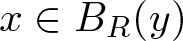$x \in B_R(y)$, one has

(1)\begin{equation} \frac{R-r}{R+r} \left(\frac{R}{R+r}\right)^{n-2} u(y) \leq u(x) \leq \frac{R+r}{R-r} \left(\frac{R}{R-r}\right)^{n-2} u(y). \end{equation}

An equivalent formulation to (Reference Moser1) was presented by Kellogg [Reference Kellogg18] which today is known in the modern theory of PDEs as the classical Harnack inequality for the Laplace operator, namely, let $\Omega'$ and Ω be open subsets in ${\mathbb{R}}^n$ so that 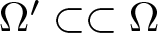$\Omega' \subset \subset \Omega$ (that is, $\overline{\Omega'}$ is a compact set contained in Ω) and let 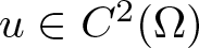$u \in C^2(\Omega)$ be a non-negative function such that 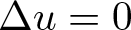$\Delta u = 0$ in Ω. Then, there is a constant $C = C(n, \Omega', \Omega) \gt 0$, depending only on n, $\Omega'$ and Ω, such that

\begin{equation*} \sup_{\Omega'} u \leq C \inf_{\Omega'} u. \end{equation*}

Years later, the estimate (Reference Moser1) was extended to second-order uniformly elliptic linear operators with bounded coefficients, more precisely to non-negative classical (of C ² class) solutions of the equation 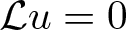${\cal L} u = 0$ in 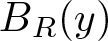$B_R(y)$, where

(2)\begin{equation} {\cal L} = a_{ij}(x) \partial_{ij} + b_i(x) \partial_i + c(x). \end{equation}

Assuming differentiability of the coefficients of ${\cal L}$, Lichtenstein [Reference Lichtenstein23] and Feller [Reference Feller12] proved a Harnack inequality in dimensions n = 2 and $n \geq 3$, respectively. Posteriorly, Serrin [Reference Serrin31] weakened considerably the smoothness assumption on the coefficients of ${\cal L}$.

A fundamental step was taken in the early 60s when Moser [Reference Moser27] established a Harnack inequality for non-negative weak solutions of the non-homogeneous elliptic equation 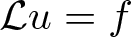${\cal L} u = f$ in an open set Ω when ${\cal L}$ is the divergence type operator without zero-order term

\begin{equation*} {\cal L} = \partial_i( a_{ij}(x) \partial_j). \end{equation*}

Precisely, given 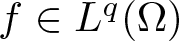$f \in L^q(\Omega)$ with 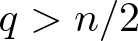$q \gt n/2$ and $B = B_{2R}(y) \subset \Omega$, there is a constant 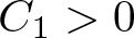$C_1 \gt 0$ such that, for any non-negative weak solution 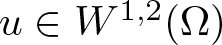$u \in W^{1,2}(\Omega)$ of 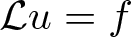${\cal L} u = f$ in Ω,

(3)\begin{equation} \sup_{B_R(y)} u \leq C_1 \left( \inf_{B_R(y)} u + R^{2-n/q} \Vert f \Vert_{L^q(B)} \right). \end{equation}

This outcome is a central cornerstone in the De Giorgi–Nash–Moser’s classical theory developed in [Reference De Giorgi9, Reference Mitidieri24, Reference Nash29] for second-order linear elliptic equations in divergence form. We refer for example to [Reference Gilbarg and Trundiger15] for the precise statement and a complete proof of (3). A remarkable fact, mentioned by DiBenedetto in [Reference DiBenedetto10] and DiBenedetto and Trudinger in [Reference DiBenedetto and Trudinger11], is that the estimate (3) can be deduced from a local boundedness of u previously obtained by De Giorgi in [Reference De Giorgi9]. For related results involving linear and non-linear elliptic operators in divergence form, we refer to Serrin [Reference Serrin32] and Trudinger [Reference Trudinger34].

Another important milestone was the establishment by Krylov and Safonov [Reference Krylov and Safonov19, Reference Krylov and Safonov20, Reference Safonov30] of the so-called Harnack–Krylov–Safonov inequality satisfied for strong solutions of the homogeneous problem 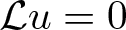${\cal L} u = 0$ in Ω considering non-divergence uniformly elliptic operators. Precisely, let $u \in W^{2,n}(\Omega)$ be a non-negative strong solution of the equation 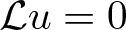${\cal L}u=0$ in Ω, where the operator ${\cal L}$ is as (2). Then, for any ball $B_{2R}(y) \subset \Omega$, it was proved that

\begin{equation*} \sup_{B_R(y)} u \leq C_1 \inf_{B_R(y)} u \end{equation*}

for a constant 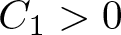$C_1 \gt 0$ independent of u. The proof of this inequality uses two key ingredients.

The first of them is the local maximum principle:

Let $u \in W^{2,n}(\Omega)$ be a function such that 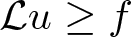${\cal L}u\geq f$ almost everywhere in Ω, where 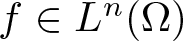$f\in L^n(\Omega)$. Then, for any ball $B = B_{2R}(y) \subset \Omega$ and p > 0, we have

\begin{equation*} \sup_{B_R(y)} u \leq \bar{C}_1 \left( \left(\frac{1}{\vert B \vert} \int_{B} (u^+)^p \right)^{\frac{1}{p}} + R ||f||_{L^n(B)} \right) \end{equation*}

for a constant 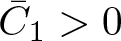$\bar{C}_1 \gt 0$ independent of u and f.

The second one is the weak Harnack inequality.

Let $u \in W^{2,n}(\Omega)$ be a non-negative function such that 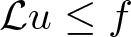${\cal L}u \leq f$ almost everywhere in Ω, where 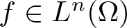$f\in L^n(\Omega)$. Then, for any ball $B = B_{2R}(y) \subset \Omega$, there are positive constants $\tilde{C}_1$ and p, also independent of u and f, such that

\begin{equation*} \left( \frac{1}{|B_R(y)|} \int_{B_R(y)} u^p\right)^{\frac{1}{p}} \leq \tilde{C}_1 \left( \inf_{B_R(y)} u + R ||f||_{L^n(B)}\right). \end{equation*}

The Harnack–Krylov–Safonov inequality and the two above tools are the basis of the theory of strong solutions for elliptic equations in non-divergence form, just as the De Giorgi–Nash–Moser regularity theory is a pillar in the study of weak solutions for equations in divergence form. For a detailed proof of them, we refer to the book [Reference Gilbarg and Trundiger15], more specifically, to corollary 9.25, theorem 9.20, and theorem 9.22.

During the last four decades, there have been many efforts to extend the well-developed theory of scalar elliptic equations to linear and non-linear elliptic systems of second order. For a complete account of regularity theory for weakly coupled cooperative elliptic systems involving operators in divergence form, we refer to the Giaquinta’s book [Reference Giaquinta14] and for systems of same kind involving operators in non-divergence form, we quote the works by Arapostathis, Ghosh, Marcus [Reference Arapostathis and Ghosh1], Chen and Zhao [Reference Chen and Zhao6], Muscalu [Reference Muscalu28], and also Busca and Sirakov [Reference Busca and Sirakov4] where Aleksandrov-Bakelman-Pucci (ABP) maximum principles and Harnack inequalities are obtained for systems involving fully non-linear operators. For different estimates of solutions of elliptic systems, we also refer to the recent works [Reference Kamburov and Sirakov17, Reference Sirakov33].

On the other hand, fairly little is known about elliptic estimates for strongly coupled non-linear elliptic systems, even considering linear operators in divergence form. This work is a contribution towards local boundedness and Harnack inequality for weak solutions of non-homogeneous Lane–Emden systems, perhaps the more famous prototypes of non-linear systems with two equations, involving divergence operators and homogeneous growth. More specifically, consider the system

(4)\begin{equation} \left\{ \begin{array}{ll} -{\cal L}_1u = \lambda\rho(x)\vert v\vert^{\alpha-1}v + f(x) & {\rm in} \ \ \Omega,\\ -{\cal L}_2v = \mu\tau(x)\vert u\vert^{\beta-1}u + g(x) & {\rm in} \ \ \Omega,\\ \end{array} \right. \end{equation}

where 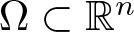$\Omega \subset \mathbb{R}^n$ is an open set, $n \geq 2$, 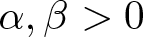$\alpha, \beta \gt 0$, 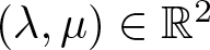$(\lambda, \mu) \in \mathbb{R}^2$ and $f,g : \Omega \rightarrow \mathbb{R}$ are measurable functions.

The system (4) is said to have homogeneous (resp. sub-homogeneous, super-homogeneous) growth if 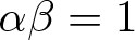$\alpha \beta=1$ (resp. 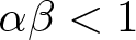$\alpha \beta \lt 1$, 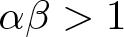$\alpha \beta \gt 1$). The notion of homogeneous growth is motivated by the following property when $f \equiv 0$ and $g \equiv 0$, which is a natural extension of the scalar case: if (u, v) is a solution of (4), then 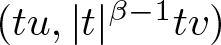$(tu, \vert t \vert^{\beta-1} t v)$ is too for every $t \in \mathbb{R}$. This is also supported by the study on principal Dirichlet eigenvalues associated with (4) carried out in [Reference Montenegro25]. Furthermore, there is an extensive literature devoted to existence and non-existence of solutions for sub-homogeneous and super-homogeneous Lane–Emden systems in parallel to corresponding scalar problems within the sublinear and superlinear contexts, respectively. As examples of some references, we mention [Reference Felmer and Martínez13, Reference Montenegro25] for sub-homogeneous systems and [Reference Clément, de Figueiredo and Mitidieri7, Reference de Figueiredo and Felmer8, Reference Hulshof and van der Vorst16, Reference Mitidieri24] for super-homogeneous ones, among many others.

Taking into account that homogeneous Lane–Emden systems are a non-linear counterpart of linear elliptic equations, recently motivated by the existence of principal Dirichlet eigenvalues for Lane–Emden systems involving non-divergence operators on general bounded domains and also by the works [Reference Berestycki, Nirenberg and Varadhan3, Reference Leite and Montenegro21, Reference Montenegro25], the authors started in [Reference Leite and Montenegro22] the developing of Lⁿ elliptic theory for strong solutions of such systems involving linear operators in non-divergence form, see theorem 2.1 for an ABP estimate, theorem 4.1 for a local boundedness result, and theorem 5.1 for a Harnack–Krylov–Safonov inequality.

The first purpose of our work is to establish a local boundedness theorem for systems of type (4) in the plane with homogeneous growth, considering uniformly elliptic operators ${\cal L}_k$ in general divergence form as

\begin{equation*} {\cal L}_k = \partial_i\left(a^k_{ij}(x) \partial_j + b^k_i(x)\right) + c^k_i(x)\partial_i + d^k(x). \end{equation*}

Secondly, as an application of the local boundedness, we establish a Harnack type inequality for non-negative weak solutions of (4). In a nutshell, our estimates take the following forms for $B = B_{2R}(y) \subset \Omega$ and $\alpha\leq 1$ (see the precise statements in theorems 3.1 and 3.2 of §3):

The weak local boundedness:

\begin{equation*} \sup_{B_{R}(y)} \vert u \vert + \sup_{B_{R}(y)} \vert v \vert^\alpha \leq C \left( R^{-2/p} \Vert u \Vert_{L^p(B)} + R^{-2\alpha/p} \Vert v \Vert^{\alpha}_{L^p(B)} + K(y,R, \alpha, f,g) \right). \end{equation*}

The Harnack type inequality:

\begin{equation*} \sup_{B_{R}(y)} u + \sup_{B_{R}(y)} v^\alpha \leq C_1 \left( \inf_{B_{R}(y)} u + \inf_{B_{R}(y)} v^\alpha + K(y,R, \alpha, f,g) \right), \end{equation*}

where $K(y,R, \alpha, f,g)$ is introduced in the final of the next section.

The leading idea of the proof of the above local boundedness consists in using De Giorgi–Nash–Moser iteration techniques in an appropriate manner in two variables in order to achieve the full range of powers 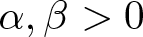$\alpha, \beta \gt 0$ with 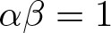$\alpha \beta = 1$. Our result is complete in the sense that it extends entirely the corresponding one when n = 1 (see, for instance, theorem 8.17 of [Reference Gilbarg and Trundiger15]). In higher dimensions, due to the restriction of the method, counterparts can be obtained under additional conditions in the ranges of α and β.

The remainder of the article is organized into four sections. In §2, we introduce some basic notations and the framework needed to state and prove the two main results. In §3, we present the precise statement of both inequalities. Section 4 is devoted to the proof of the weak local boundedness, while §5 focuses on proving the Harnack inequality for the system (4).

2. General assumptions and structural inequalities

In what follows we introduce some notations and assumptions that will be assumed in the statements of theorems. Some of the notations are borrowed from [Reference Gilbarg and Trundiger15].

Let Ω be an open set of $\mathbb{R}^2$ and let ${\cal L}_k$ ( 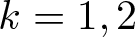$k =1, 2$) be the second-order uniformly elliptic operator in general divergence form

\begin{equation*} {\cal L}_k = \partial_i\left(a^k_{ij}(x) \partial_j + b^k_i(x)\right) + c^k_i(x)\partial_i + d^k(x), \end{equation*}

where the coefficients $a^k_{ij}$, $b^k_i$, $c^k_i$, and d^k are measurable functions that satisfy the assumptions of ellipticity and boundedness

(5)\begin{equation} a^k_{ij}(x) \xi_i \xi_j \geq a_k |\xi|^2,\ \ \forall \xi \in \mathbb{R}^2,\ x \in \Omega, \end{equation}

(6)\begin{equation} \sum\vert a^k_{ij}(x)\vert^2 \leq A_k^2,\ \ a_k^{-2}\sum(\vert b_i^k(x)\vert^2 + c^k_i(x)) + a_k^{-1}\vert d_k(x)\vert \leq \nu_k^2,\ \ \forall x \in \Omega \end{equation}

for constants 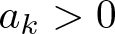$a_k \gt 0$ and 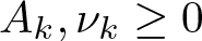$A_k, \nu_k \geq 0$. It is also assumed without loss of generality that 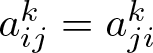$a^k_{ij}=a^k_{ji}$ for all $i,j,k = 1,2$.

The functions ρ, τ, f, and g are taken in 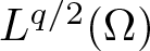$L^{q/2}(\Omega)$ for some q > 2, parameters λ and µ in $\mathbb{R}$ and positive powers α and β such that 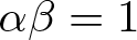$\alpha \beta = 1$.

A couple $(u,v)\in (W^{1,2}(\Omega))^2$ is said to be a weak (sub)solution of the problem (4) if, for any non-negative test function 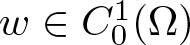$w\in C^1_0(\Omega)$,

\begin{equation*} \int_{\Omega}a^1_{ij} \frac{\partial u}{\partial x_j}\frac{\partial w}{\partial x_i} + b^1_i u\frac{\partial w}{\partial x_i} - c^1_i \frac{\partial u}{\partial x_i} w - d^1 u w\, dx\ (\leq) = \int_{\Omega} \left( \lambda\rho(x)\vert v\vert^{\alpha-1}v + f(x) \right)w\, dx, \end{equation*}

\begin{equation*} \int_{\Omega}a^2_{ij} \frac{\partial u}{\partial x_j}\frac{\partial w}{\partial x_i} + b^2_i u\frac{\partial w}{\partial x_i} - c^2_i \frac{\partial u}{\partial x_i} w - d^2 u w\, dx\ (\leq) = \int_{\Omega} \left( \mu\tau(x)\vert u\vert^{\beta-1}u + g(x) \right)w\, dx. \end{equation*}

Let us rewrite the above system in the weak sense as

(7)\begin{equation} \left\{ \begin{array}{llll} -\partial_i A_i^1(x,u,\nabla u)\ (\leq) = B^1(x,u,v,\nabla u) & {\rm in} \ \ \Omega,\\ -\partial_i A_i^2(x,v,\nabla v)\ (\leq) = B^2(x,u,v,\nabla v) & {\rm in} \ \ \Omega,\\ \end{array} \right. \end{equation}

where $A^k: \Omega \times \mathbb{R} \times \mathbb{R}^2 \rightarrow \mathbb{R}^{2}$ and $B^k: \Omega \times \mathbb{R}^2 \times \mathbb{R}^2 \rightarrow\mathbb{R}$ are for 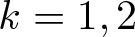$k=1,2$ given by

\begin{equation*} \begin{array}{l} A_i^k(x,z,\eta) = a_{ij}^k(x) \eta_j + b_i^k(x) z,\\ B^1(x,z,w,\eta)= c^1_i(x) \eta_i + d^1(x)z + \lambda \rho(x) \vert w\vert^{\alpha-1} w + f(x),\\ B^2(x,z,w,\eta)= c^2_i(x) \eta_i + d^2(x) w + \mu \tau(x) \vert z\vert^{\beta-1}z + g(x). \end{array} \end{equation*}

Let 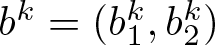$b^k = (b^k_1, b^k_2)$ and 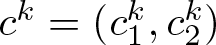$c^k = (c^k_1, c^k_2)$, 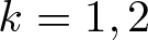$k=1,2$. Set for each 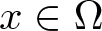$x \in \Omega$ and constants 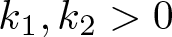$k_1,k_2 \gt 0$,

\begin{equation*} \overline{z}=\vert z\vert + k_1,\ \ \ \overline{b}^1(x) = a_1^{-2} \left( \vert b^1(x) \vert^2 + \vert c^1(x) \vert^2 \right) + a_1^{-1} \left( \vert d^1(x) \vert + k_1^{-1}\vert f(x) \vert \right), \end{equation*}

\begin{equation*} \overline{w}=\vert w\vert + k_2,\ \ \ \overline{b}^2(x) = a_2^{-2} \left( \vert b^2(x) \vert^2 + \vert c^2(x) \vert^2 \right) + a_2^{-1} \left( \vert d^2(x) \vert + k_2^{-1}\vert g(x) \vert \right). \end{equation*}

Denoting now the matrix 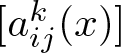$[a_{ij}^k(x)]$ by 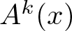$A^k(x)$. By dividing the kth equation of (4) by $a_k/2$, we can assume that 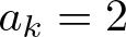$a_k = 2$. Assuming this condition, we gather the following structural inequalities:

(8)\begin{equation} \begin{array}{l} \vert A^k(x,z,\eta)\vert \leq \vert A^k(x) \vert \vert\eta\vert + 2(\overline{b}^k(x))^{\frac{1}{2}} \overline{z},\\ \eta \cdot A^k(x,z,\eta) \geq \vert\eta\vert^2 - 2\overline{b}^k(x) \overline{z}^2,\\ \vert\overline{z} B^1(x,z,w,\eta)\vert \leq \varepsilon \vert\eta\vert^2 + \frac{1}{\varepsilon}\overline{b}^1(x) \overline{z}^2 + \vert\lambda\vert\rho(x)\vert w\vert^{\alpha}\overline{z},\\ \vert\overline{w} B^2(x,z,w,\eta)\vert \leq \varepsilon \vert\eta\vert^2 + \frac{1}{\varepsilon}\overline{b}^2(x) \overline{w}^2 + \vert\mu\vert\tau(x)\vert z\vert^{\beta}\overline{w} \end{array} \end{equation}

for any number 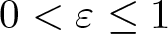$0 \lt \varepsilon \leq 1$.

For a fixed ball $B = B_{2R}(y) \subset \Omega$, we consider the constant

\begin{equation*} K(y,R, \alpha, f, g) = a_1^{-1} R^{2\delta} \Vert f\Vert_{L^{q/2}(B)} + a_2^{-\alpha} R^{2 \alpha \delta} \Vert g\Vert_{L^{q/2}(B)}^\alpha, \end{equation*}

where $\delta = 1 - 2/q$.

3. Main statements

From now on, we will consider all notations introduced in the previous section. Our main result is the following local boundedness for weak solutions of non-homogeneous Lane–Emden systems:

Theorem 3.1. Let 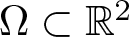$\Omega \subset \mathbb{R}^2$ be an open set, let ${\cal L}_k$ ( 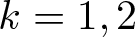$k=1,2$) be an operator satisfying the conditions (5) and (6) and assume that $\rho, \tau, f, g \in L^{q/2}(\Omega)$ for some q > 2 and 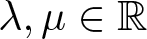$\lambda, \mu \in \mathbb{R}$. Let also 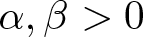$\alpha,\beta \gt 0$ be such that 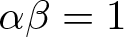$\alpha \beta=1$ and assume that $\alpha \leq 1$.

Let $(u,v) \in (W^{1,2}(\Omega))^2$ be a subsolution of the Lane–Emden system (4). Then, for any ball $B=B_{2R}(y) \subset \Omega$ and p > 1, we have

(9)\begin{align} \sup_{B_{R}(y)} \vert u \vert + \sup_{B_{R}(y)} \vert v \vert^\alpha \leq C \left(R^{-2/p}\Vert u\Vert_{L^p(B)} + R^{-2\alpha/p}\Vert v\Vert^{\alpha}_{L^p(B)} + K(y,R, \alpha, f, g) \right)\nonumber\\ \end{align}

for a constant $C = C(A_k/a_k,\nu_k R, \lambda, \mu, \Vert \rho \Vert_{L^{q/2}(\Omega)}, \Vert \tau \Vert_{L^{q/2}(\Omega)}, \alpha, p, q) \gt 0$.

As an application of this theorem, we obtain the Harnack type estimate for Lane–Emden systems:

Theorem 3.2. Let $\Omega, {\cal L}_k$ ( 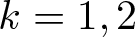$k=1,2$), $\rho, \tau, f, g, \lambda, \mu, \delta$, and α be as in theorem 3.1. Assume, moreover, that ρ and τ are non-negative functions in Ω and 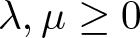$\lambda, \mu \geq 0$.

Let $(u,v) \in (W^{1,2}(\Omega))^2$ be a non-negative weak solution of the Lane–Emden system (4). Then, for any ball $B=B_{4R}(y) \subset \Omega$, we have

\begin{equation*} \sup_{B_{R}(y)} u + \sup_{B_{R}(y)} v^\alpha \leq C_1 \left(\inf_{B_{R}(y)} u + \inf_{B_{R}(y)} v^\alpha + K(y,2 R, \alpha, f, g)\right) \end{equation*}

for a constant $C_1 = C_1(A_k/a_k, \nu_k R, \lambda, \mu, \Vert \rho \Vert_{L^{q/2}(\Omega)}, \Vert \tau \Vert_{L^{q/2}(\Omega)}, \alpha, q) \gt 0$.

Note that the estimate above can alternatively be rephrased as:

Corollary 3.1. Let 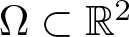$\Omega \subset \mathbb{R}^2$ be an open set. Under the assumptions of theorem 3.2, we have, for any open 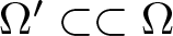$\Omega' \subset \subset \Omega$,

\begin{equation*} \sup_{\Omega'} u + (\sup_{\Omega'} v )^\alpha \leq C_2 \left(\inf_{\Omega'} u + (\inf_{\Omega'} v )^\alpha + \Vert f \Vert_{L^{q/2}(\Omega)} + \Vert g \Vert^\alpha_{L^{q/2}(\Omega)} \right) \end{equation*}

for a constant $C_2 = C_2(A_k/a_k, \nu_k, \lambda, \mu, \Vert \rho \Vert_{L^{q/2}(\Omega)}, \Vert \tau \Vert_{L^{q/2}(\Omega)}, \alpha, q, \Omega', \Omega) \gt 0$.

As a direct consequence of the above local boundedness and Harnack inequality, we derive counterparts for weak solutions of biharmonic equations of the type

(10)\begin{equation} (-\Delta)^2 v=\lambda\rho(x)v + f(x)\ \ {\rm in} \ \ \Omega \end{equation}

on open sets 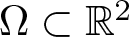$\Omega \subset \mathbb{R}^2$, which are in correspondence with systems of the form

(11)\begin{equation} \left\{ \begin{array}{ll} -\Delta u = \lambda\rho(x) v + f(x) & {\rm in} \ \ \Omega,\\ -\Delta v = u & {\rm in} \ \ \Omega. \end{array} \right. \end{equation}

A priori estimates for biharmonic functions ( $f \equiv 0$ and λ = 0) and, more generally, for poly-harmonic functions are very classical problems and well studied. For instance, Busca and Sirakov established in [Reference Busca and Sirakov4] a Harnack inequality for classical solutions of the poly-harmonic equation

\begin{equation*} (-\Delta)^N v = \lambda\rho(x)v + f(x)\ \ {\rm in} \ \ \Omega \subset \mathbb{R}^n, \end{equation*}

where 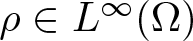$\rho \in L^{\infty}(\Omega)$. Later, Caristi and Mitidieri [Reference Caristi and Mitidieri5] obtained a Harnack inequality for weak solutions of (10) (i.e. N = 2) in 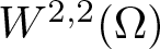$W^{2,2}(\Omega)$, where $f \equiv 0$ and ρ belongs to 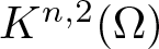$K^{n,2}(\Omega)$ the natural Kato class of potentials associated with the operator 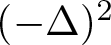$(-\Delta)^2$ (see definition 2.2 in [Reference Caristi and Mitidieri5]).

Theorem 3.1, when applied to the system (11), yields the following estimate for weak subsolutions of non-homogeneous biharmonic equations:

Corollary 3.2. Let 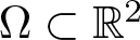$\Omega \subset \mathbb{R}^2$ be an open set and assume that $\rho, f \in L^{q/2}(\Omega)$ for some q > 2 and 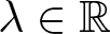$\lambda \in \mathbb{R}$.

Let 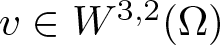$v \in W^{3,2}(\Omega)$ be a weak subsolution of the biharmonic equation (10). Then, for any ball $B=B_{2R}(y) \subset \Omega$ and p > 1, we have

\begin{equation*} \sup_{B_{R}(y)} \vert \Delta v \vert + \sup\limits_{B_{R}(y)} \vert v \vert \leq C \left(\Vert \Delta v \Vert_{L^p(B)} +\Vert v\Vert_{L^p(B)} + \Vert f\Vert_{L^{q/2}(B)}\right) \end{equation*}

for a constant $C=C(R,\lambda,\Vert \rho \Vert_{L^{q/2}(\Omega)},p,q) \gt 0$.

Here, the regularity 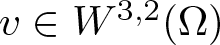$v \in W^{3,2}(\Omega)$ is used since it implies that $(u, v) \in (W^{1,2}(\Omega))^2$ where $u:= -\Delta v$.

Finally, theorem 3.2 along with Krylov’s theorem (theorem 7.1 in [Reference Busca and Sirakov4]) produces the following Harnack inequality for weak solutions of Eq. (10).

Corollary 3.3. Let 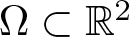$\Omega \subset \mathbb{R}^2$ be an open set and assume that $\rho, f \in L^{q/2}(\Omega)$ for some q > 2 and 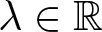$\lambda \in \mathbb{R}$. Assume, moreover, that ρ is non-negative in Ω and $\lambda \geq 0$.

Let 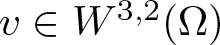$v \in W^{3,2}(\Omega)$ be a non-negative weak solution of the biharmonic equation (10) such that 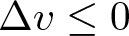$\Delta v \leq 0$ in Ω. Then, for any ball $B=B_{4R}(y)\subset\Omega$,

(12)\begin{equation} \sup_{B_{R}(y)} v\leq C_1 \left(\inf_{B_{R}(y)} v + \Vert f \Vert_{L^{q/2}(B)}\right) \end{equation}

for a constant $C_1 = C_1(R,\lambda, \Vert \rho \Vert_{L^{q/2}(\Omega)},q) \gt 0$.

In effect, theorem 3.2 gives

\begin{equation*} \sup_{B_{R}(y)} (-\Delta v)+\sup\limits_{B_{R}(y)} v\leq C \left(\inf_{B_{R}(y)} (-\Delta v)+\inf\limits_{B_{R}(y)} v + ||f||_{L^{q/2}(B)}\right), \end{equation*}

where $C = C(R,\lambda, \Vert \rho \Vert_{L^{q/2}(\Omega)}, q)$ is a positive constant. Also, by Krylov’s theorem, there exists a constant $C_0 = C_0(R) \gt 0$ such that

\begin{equation*} \inf_{B_{R}(y)} (-\Delta v) \leq C_0 \inf_{B_{R}(y)} v. \end{equation*}

Joining these two inequalities, it follows readily the estimate (12).

4. Proof of theorem 3.1

By assumption, it is assumed that $\alpha \leq 1$, and so $\beta \geq 1$ since 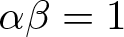$\alpha\beta=1$. We suppose initially that R = 1 and k ₁ and k ₂ are arbitrary positive constants. Let us define for 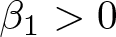$\beta_1 \gt 0$ and a non-negative cut-off function $\varphi\in C^1_0(B_4(y))$ with 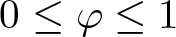$0 \leq \varphi \leq 1$ in $B_4(y)$, the functions

\begin{equation*} u_0=\varphi^2 \overline{u}^{\beta_1}\ (\overline{u}=u+k_1)\ \ {\rm and }\ \ v_0=\varphi^{2\beta} \overline{v}^{\beta_1}\ (\overline{v}=v+k_2). \end{equation*}

Using u ₀ and v ₀ as test functions in the respective equations of (7), we obtain the two inequalities

(13)\begin{align} &\beta_1\int_{\Omega}\varphi^2\overline{u}^{\beta_1-1}\nabla u\cdot A^1(x,u,\nabla u)\, dx+2\int_{\Omega}\varphi\nabla\varphi\cdot A^1(x,u,\nabla u)\overline{u}^{\beta_1}\, dx\nonumber\\ &\quad \leq -\int_{\Omega}\varphi^2\overline{u}^{\beta_1}B^1(x,u,v,\nabla u)\, dx, \end{align}

(14)\begin{align} &\beta_1\int_{\Omega}\varphi^{2\beta}\overline{v}^{\beta_1-1}\nabla v\cdot A^2(x,v,\nabla v)\, dx+2\beta\int_{\Omega}\varphi^{2\beta-1}\nabla\varphi\cdot A^2(x,v,\nabla v)\overline{v}^{\beta_1}\, dx\nonumber\\ &\quad \leq -\int_{\Omega}\varphi^{2\beta}\overline{v}^{\beta_1}B^2(x,u,v,\nabla v)\, dx. \end{align}

From the structural inequalities (8), for any 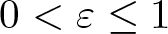$0 \lt \varepsilon \leq 1$, we have

\begin{equation*} \vert \varphi\nabla\varphi\cdot A^1(x,u,\nabla u)\overline{u}^{\beta_1}\vert\leq \frac{\varepsilon}{2}\varphi^2\overline{u}^{\beta_1-1}\vert\nabla u\vert^2+ (1+ \frac{\vert A^1(x) \vert^2}{2\varepsilon})\vert\nabla\varphi\vert^2 \overline{u}^{\beta_1+1} +\overline{b}^1\varphi^2\overline{u}^{\beta_1+1}, \end{equation*}

\begin{equation*} \vert\varphi^2\overline{u}^{\beta_1} B^1(x,u,v,\nabla u)\vert\leq\varepsilon\varphi^2\overline{u}^{\beta_1-1}\vert\nabla u\vert^2+\frac{1}{\varepsilon}\overline{b}^1\varphi^2\overline{u}^{\beta_1+1}+\varphi^2\overline{u}^{\beta_1}\vert\lambda\rho(x)\vert\vert v\vert^{\alpha}, \end{equation*}

\begin{equation*} \varphi^2\overline{u}^{\beta_1-1}\nabla u\cdot A^1(x,u,\nabla u)\geq \varphi^2\overline{u}^{\beta_1-1}\vert\nabla u\vert^2-2(\overline{b}^1)\varphi^2\overline{u}^{\beta_1+1}, \end{equation*}

\begin{align*} \vert \varphi^{2\beta-1}\nabla\varphi\cdot A^2(x,v,\nabla v)\overline{v}^{\beta_1}\vert&\leq \frac{\varepsilon}{2}\varphi^{2(2\beta-1)}\overline{v}^{\beta_1-1}\vert\nabla v\vert^2+ (1+ \frac{\vert A^2(x) \vert^2}{2\varepsilon}) \vert\nabla\varphi\vert^2 \overline{v}^{\beta_1+1} \\ &\quad +\overline{b}^2\varphi^{2(2\beta-1)}\overline{v}^{\beta_1+1}, \end{align*}

\begin{equation*} \vert\varphi^{2\beta}\overline{v}^{\beta_1} B^2(x,u,v,\nabla v)\vert\leq\varepsilon\varphi^{2\beta}\overline{v}^{\beta_1-1}\vert\nabla v\vert^2+\frac{1}{\varepsilon}\overline{b}^2\varphi^{2\beta}\overline{v}^{\beta_1+1}+\varphi^{2\beta}\overline{v}^{\beta_1}\vert\mu\tau(x)\vert\vert u\vert^{\beta}, \end{equation*}

\begin{equation*} \varphi^{2\beta}\overline{v}^{\beta_1-1}\nabla v\cdot A^2(x,v,\nabla v)\geq \varphi^{2\beta}\overline{v}^{\beta_1-1}\vert\nabla v\vert^2-2(\overline{b}^2)\varphi^{2\beta}\overline{v}^{\beta_1+1}. \end{equation*}

By taking $\varepsilon=\min\{1,\beta_1/4\}$, we then deduce from (13) that

(15)\begin{align} \int_{\Omega}\varphi^2\overline{u}^{\beta_1-1}\vert\nabla u\vert^2\, dx&\leq C(\beta_1)\int_{\Omega}(\overline{b}^1\varphi^2+(1+\vert A^1(x) \vert^2)\vert\nabla\varphi\vert^2)\overline{u}^{\beta_1+1}\, dx\nonumber\\ &\quad +\int_{\Omega}\varphi^2\overline{u}^{\beta_1}\vert\lambda\rho(x)\vert\vert v\vert^{\alpha}\, dx \end{align}

and from (14),

(16)\begin{align} \int_{\Omega}\varphi^{2\beta}\overline{v}^{\beta_1-1}\vert\nabla v\vert^2&\leq C(\beta_1)\, dx\int_{\Omega}(\overline{b}^2\varphi^{2\beta}+(1+\vert A^2(x) \vert^2)\vert\nabla\varphi\vert^2)\overline{v}^{\beta_1+1}\, dx\nonumber\\ &\quad +\int_{\Omega}\varphi^{2\beta}\overline{v}^{\beta_1}\vert\mu\tau(x)\vert\vert u\vert^{\beta}\, dx, \end{align}

where 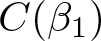$C(\beta_1)$ is bounded if β ₁ is bounded far from zero.

Now define

\begin{equation*} w_0=\overline{u}^{(\beta_1+1)/2} \ \ {\rm and}\ \ z_0=\overline{v}^{(\beta_1+1)/2}. \end{equation*}

Setting 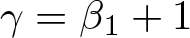$\gamma=\beta_1+1$, Eqs. (15) and (16) can be rewritten, respectively, as

(17)\begin{align} \int_{\Omega}\vert\varphi\nabla w_0\vert^2\, dx&\leq C(\beta_1)\gamma^2\int_{\Omega}(\overline{b}^1\varphi^2+(1+\vert A^1(x) \vert^2)\vert\nabla\varphi\vert^2)w_0^2\, dx+\gamma^2\nonumber\\ &\quad \times \int_{\Omega}\varphi^2w_0^{\frac{2\beta_1}{\beta_1+1}}\vert\lambda\rho(x)\vert\vert v\vert^{\alpha}\, dx, \end{align}

(18)\begin{align} \int_{\Omega}\vert\varphi^{\beta}\nabla z_0\vert^2\, dx&\leq C(\beta_1)\gamma^2\int_{\Omega}(\overline{b}^2\varphi^{2\beta}+(1+\vert A^2(x) \vert^2)\vert\nabla\varphi\vert^2)z_0^2\, dx+\gamma^2\nonumber\\ &\quad\times\int_{\Omega}\varphi^{2\beta}z_0^{\frac{2\beta_1}{\beta_1+1}}\vert\mu\tau(x)\vert\vert u\vert^{\beta}\, dx. \end{align}

On the other hand, by Sobolev embedding, we have

\begin{equation*} \Vert\varphi w_0\Vert^2_{L^{2\chi}(\Omega)}\leq \tilde{C}_1\int_{\Omega}(\vert\varphi\nabla w_0\vert^2+\vert w_0\nabla\varphi\vert^2)\, dx \end{equation*}

and

\begin{equation*} \Vert\varphi^{\beta} z_0\Vert^2_{L^{2\chi}(\Omega)}\leq \tilde{C}_2\int_{\Omega}(\vert\varphi^\beta\nabla z_0\vert^2+\vert z_0\nabla\varphi\vert^2)\, dx, \end{equation*}

where 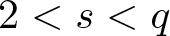$2 \lt s \lt q$, $\chi=s/(s-2)$, 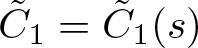$\tilde{C}_1 = \tilde{C}_1(s)$, and $\tilde{C}_2 = \tilde{C}_2(\beta,s)$.

By using Hölder’s inequality followed by interpolation inequality, for any 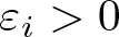$\varepsilon_i \gt 0$ with $i=1,\ldots, 4$, we get

\begin{equation*} \int_{\Omega}\overline{b}^1(\varphi w_0)^2\, dx\leq\Vert\overline{b}^1\Vert_{L^{q/2}(\Omega)}\left(\varepsilon_1\Vert\varphi w_0\Vert_{L^{2\chi}(\Omega)}+\varepsilon_1^{-\sigma}\Vert\varphi w_0\Vert_{L^2(\Omega)}\right)^2, \end{equation*}

\begin{equation*} \int_{\Omega}\overline{b}^2(\varphi^\beta z_0)^2\, dx\leq\Vert\overline{b}^2\Vert_{L^{q/2}(\Omega)}\left(\varepsilon_2\Vert\varphi^\beta z_0\Vert_{L^{2\chi}(\Omega)}+\varepsilon_2^{-\sigma}\Vert\varphi^\beta z_0\Vert_{L^2(\Omega)}\right)^2, \end{equation*}

\begin{align*} \int_{\Omega}\varphi^2w_0^{\frac{2\beta_1}{\beta_1+1}}\vert\lambda\rho(x)\vert\vert v\vert^{\alpha}\, dx&\leq \Vert\lambda\rho\Vert_{L^{q/2}(\Omega)}\frac{\beta_1}{\beta_1+1}\left(\varepsilon_3\Vert\varphi w_0\Vert_{L^{2\chi}(\Omega)}\right.\\ &\quad +\left.\varepsilon_3^{-\sigma}\Vert\varphi w_0\Vert_{L^2(\Omega)}\right)^2\\ &\quad +\ \Vert\lambda\rho\Vert_{L^{q/2}(\Omega)}\frac{1}{\beta_1+1}\left(\varepsilon_4\Vert\varphi z_0^\alpha\Vert_{L^{2\chi}(\Omega)}\right.\\ &\quad +\left.\varepsilon_4^{-\sigma}\Vert\varphi z_0^\alpha\Vert_{L^2(\Omega)}\right)^2, \end{align*}

and using that $\beta\geq 1$ and 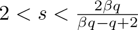$2 \lt s \lt \frac{2\beta q}{\beta q-q+2}$, for any 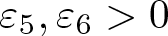$\varepsilon_5, \varepsilon_6 \gt 0$, we also have

\begin{align*} \int_{\Omega}\varphi^{2\beta}z_0^{\frac{2\beta_1}{\beta_1+1}}\vert\mu \tau(x)\vert \vert u\vert^{\beta}\, dx&\leq \Vert\mu\tau\Vert_{L^{q/2}(\Omega)}\frac{\beta_1}{\beta_1+1}\left(\varepsilon_5\Vert\varphi^\beta z_0\Vert_{L^{2\chi}(\Omega)}\right.\\ &\quad +\left.\varepsilon_5^{-\sigma}\Vert\varphi^\beta z_0\Vert_{L^2(\Omega)}\right)^2\\ &\quad +\ \Vert\mu\tau\Vert_{L^{q/2}(\Omega)}\frac{1}{\beta_1+1}\left(\varepsilon_6\Vert\varphi w_0\Vert_{L^{2\chi}(\Omega)}\right.\\ &\quad +\left.\varepsilon_6^{-\sigma_0}\Vert\varphi w_0\Vert_{L^2(\Omega)}\right)^{2\beta}, \end{align*}

where 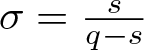$\sigma=\frac{s}{q-s}$ and $\sigma_0 = \frac{s(\beta q-q+2)}{s(q-2)-\beta q(s-2)}$. Here we point out that it is necessary to choose s close enough to 2 so that σ ₀ is positive and thus the interpolation inequality occurs for any $\beta \geq 1$.

Plugging these inequalities into (17) and (18) and choosing ɛ_i in an appropriate way for $i=1,2,3,5$, we derive

(19)\begin{align} \Vert\varphi w_0\Vert_{L^{2\chi}(\Omega)} &\leq C \left[(1+\vert\gamma\vert)^{\sigma+1}\Vert(\varphi+\vert\nabla\varphi\Vert)w_0\Vert_{L^2(\Omega)} + \varepsilon_4\Vert\varphi z_0^\alpha\Vert_{L^{2\chi}(\Omega)}\right.\nonumber\\ &\quad +\left.\varepsilon_4^{-\sigma}\Vert\varphi z_0^\alpha\Vert_{L^2(\Omega)} \right], \end{align}

(20)\begin{align} \Vert\varphi^{\beta} z_0\Vert_{L^{2\chi}(\Omega)}&\leq C \left[(1+\vert\gamma\vert)^{\sigma_0+1}\Vert(\varphi^\beta+\vert\nabla\varphi\Vert)z_0\Vert_{L^2(\Omega)}\right.\nonumber\\ &\quad +\left. \left(\varepsilon_6\Vert\varphi w_0\Vert_{L^{2\chi}(\Omega)}+\varepsilon_6^{-\sigma_0}\Vert\varphi w_0\Vert_{L^2(\Omega)}\right)^\beta \right], \end{align}

where C is bounded when β ₁ is bounded far from zero. Thus, adding up inequalities (19) and (20), conveniently choosing ɛ ₄ and ɛ ₆ and using that 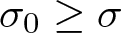$\sigma_0\geq\sigma$, we get

\begin{align*} \Vert\varphi w_0\Vert_{L^{2\chi}(\Omega)}+\Vert\varphi z_0^\alpha\Vert_{L^{2\chi}(\Omega)}&\leq C(1+\vert\gamma\vert)^{\sigma_0+1} (\Vert(\varphi+\vert\nabla\varphi\Vert)w_0\Vert_{L^2(\Omega)}\\ &\quad +\Vert(\varphi^\beta+\vert\nabla\varphi\Vert)z_0\Vert_{L^2(\Omega)}^\alpha). \end{align*}

Let $r_1,r_2$ be such that $1\leq r_1 \lt r_2\leq 3$ and fix a cut-off function φ such that $\varphi \equiv 1$ in 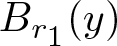$B_{r_1}(y)$, 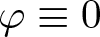$\varphi \equiv 0$ in 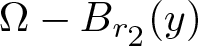$\Omega-B_{r_2}(y)$, and $\vert\nabla\varphi\vert\leq 2/(r_2-r_1)$. Then,

(21)\begin{align} &\Vert w_0\Vert_{L^{2\chi}(B_{r_1}(y))}+\Vert z_0^\alpha\Vert_{L^{2\chi}(B_{r_1}(y))}\nonumber\\ &\quad \leq \dfrac{C(1+\vert\gamma\vert)^{\sigma_0+1}}{r_2-r_1} (\Vert w_0\Vert_{L^{2}(B_{r_2}(y))}+\Vert z_0\Vert_{L^{2}(B_{r_2}(y))}^\alpha). \end{align}

Define

\begin{equation*} \Phi_u(p,r) = \left(\int_{B_r(y)}\vert\overline{u}\vert^p\, dx\right)^{\frac{1}{p}}. \end{equation*}

With this notation in mind, the inequality (21) becomes

(22)\begin{align} \Phi_u(\chi\gamma,r_1)+\left[\Phi_v(\chi\gamma\alpha,r_1)\right]^\alpha\leq\left(\frac{C(1+\vert\gamma\vert)^{\sigma_0+1}}{r_2-r_1}\right)^{\frac{2}{\vert\gamma\vert}}\left(\Phi_u(\gamma,r_2)+\left[\Phi_{v}(\gamma,r_2)\right]^\alpha\right).\nonumber\\ \end{align}

Now take p > 1 and set $\gamma=\gamma_m=\chi^mp$ and $r_m=1+2^{-m}$ for integers 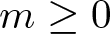$m \geq 0$. So, the inequality (22) yields

\begin{equation*} \begin{array}{rcl} \Phi_u(\chi^mp,1)+\left[\Phi_v(\chi^mp\alpha,1)\right]^\alpha &\leq &\left(C\chi\right)^{2(\sigma_0+1) \sum\limits_{k=0}^{\infty} k\chi^{-k}}(\Phi_u(p,2)+\left[\Phi_{v}(p,2)\right]^\alpha)\\ &\leq &C(\Phi_u(p,2)+\left[\Phi_{v}(p,2)\right]^\alpha), \end{array} \end{equation*}

where $C=C(s,A_k, \nu_k,q,p,\lambda,\mu,\Vert \rho \Vert_{L^{q/2}(\Omega)}, \Vert \tau \Vert_{L^{q/2}(\Omega)},\alpha)$.

Finally, letting $m \rightarrow \infty$ in the above inequality, we get

\begin{equation*} {\sup_{B_{1}(y)} \vert\overline{u}\vert}+{\left(\sup_{B_{1}(y)}\vert \overline{v}\vert\right)^\alpha} \leq C {\left(\Vert \overline{u}\Vert_{L^p(B_2(y))} +\Vert \overline{v}\Vert^{\alpha}_{L^p(B_2(y))}\right)} \end{equation*}

and hence the desired estimate (9) follows by using the transformation 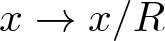$x \rightarrow x/R$.

5. Proof of theorem 3.2

The proof of the Harnack–Krylov–Safonov inequality for Lane–Emden systems in the plane is carried out by using theorem 3.1 along with the following weak Harnack inequality for supersolutions due to Trudinger (theorem 8.18 of [Reference Gilbarg and Trundiger15]):

Theorem 5.1. Let 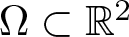$\Omega \subset \mathbb{R}^2$ be an open set and let ${\cal L}_k$ be an operator satisfying the conditions (5) and (6). Let $w \in W^{1,2}(\Omega)$ be a non-negative weak supersolution of the problem 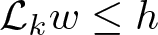${\cal L}_k w \leq h$ in Ω, where 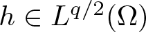$h \in L^{q/2}(\Omega)$ for some q > 2. Then, for any ball $B = B_{4R}(y) \subset \Omega$ and parameter $p \geq 1$, there is a constant $D_k = D_k(A_k/a_k,\nu_k R,p,q) \gt 0$ such that

\begin{equation*} \left( R^{-2}\int_{B_{2R}(y)} w^{p}\, dx\right)^{\frac{1}{p}} \leq D_k \left(\inf_{B_R(y)} w + a_k^{-1}R^{2\delta}||h||_{L^{q/2}(B)}\right). \end{equation*}

Proof of theorem 3.2: We first take 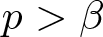$p \gt \beta$ and $D_0:= \max\{D_1, D_2^\alpha\} \gt 0$, where D_k is provided in the previous theorem for 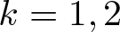$k = 1,2$. Now combining theorems 3.1 and 5.1, we obtain

\begin{align*} \sup_{B_R(y)} u + \sup_{B_R(y)} v^\alpha &\leq C \left(R^{-2/p}\Vert u\Vert_{L^p(B_{2R}(y))} + a_{1}^{-1}R^{2\delta}\Vert f\Vert_{L^{q/2}(B_{2R}(y))}\right. \\ &\quad +\,R^{-2\alpha/p}\Vert v\Vert^{\alpha}_{L^p(B_{2R}(y))} \\ & \quad+\, \left. a_{2}^{-\alpha}R^{2\alpha\delta}\Vert g\Vert^\alpha_{L^{q/2}(B_{2R}(y))}\right)\\ &\leq CD_0 \left(\inf_{B_{R}(y)} u + \inf_{B_{R}(y)} v^\alpha + a_{1}^{-1}R^{2\delta}||f||_{L^{q/2}(B)}\right.\\ &\quad +\left. a_{2}^{-\alpha}R^{2\alpha\delta}||g||^\alpha_{L^{q/2}(B)}\right), \end{align*}

where $CD_0= C_1(A_k/a_k,\nu_k R,\lambda,\mu,\Vert \rho \Vert_{L^{q/2}(\Omega)}, \Vert \tau \Vert_{L^{q/2}(\Omega)},\alpha,p,q)$ and so we conclude the proof.