Introduction
In the second half of the last century, devices based on organic materials were presented for the first time, which led to increased interest and intensified studies in this field. Such devices are organic light emitting diodes (OLED [Reference Tang and VanSlyke1, Reference Burroughes, Bradley, Brown, Marks, Mackay, Friend, Burns and Holmes2]), solar cells [Reference Chamberlain3, Reference Wöhrle and Meissner4], detectors [Reference McCormack, Tong and Cooke5], transistors [Reference Koezuka, Tsumura and Ando6, Reference Tsumura, Koezuka and Ando7], and lasers [Reference Kozlov, Bulovic, Burrows and Forrest8, Reference Schön, Kloc, Dodabalapur and Batlogg9, Reference Koschorreck, Gehlhaar, Lyssenko, Swoboda, Hoffmann and Leo10]. In particular, the first demonstration of an optically pumped polymer microcavity (MC) laser [Reference Tessler, Denton and Friend11] caused the field of solid-state organic lasers to become a major research area.
It is highly desirable to exchange optical pumping of organic solid-state MC lasers by electrical pumping to exploit all advantages offered by these systems. Nevertheless, despite intensive studies, it was not yet possible to realize an electrically driven organic solid-state laser [Reference Samuel, Namdas and Turnbull12] at room temperature. The main challenges for electrical pumping are related to the very high current densities [Reference Chakaroun, Coens, Fabre, Gourdon, Solard, Fischer, Bourdrioua and Lee13] required to reach lasing threshold (LT). This is mostly due to strongly enhanced exciton–exciton annihilation, polaron absorption, and population of triplet states. The latter do not show fluorescence and, therefore, cannot directly contribute to the lasing process. This leads to an immense loss of pump intensity of at least 75%. Additionally, the relatively poor stability of organic materials, the absorption of the metal contacts, and the influence of the charge carriers (cc) have to be considered.
There are numerous estimations of a minimal current density needed to reach LT. The reported values range from a few hundred up to a few thousand A/cm2 depending on the model and device geometry [Reference Setoguchi and Adachi14]. Few years ago, different reports [Reference Kasemann, Brückner, Fröb and Leo16, Reference Nakanotani, Oyamada, Kawamura, Sasabe and Adachi17, Reference Nakanotani, Sasabe and Adachi18] stated current densities in the range of 1 kA/cm2; a more recent paper [Reference Chime, Bensmida, Chakaroun, Lee, Nkwawo and Fischer19] showed current densities up to 2 kA/cm2 under pulsed excitation without reaching the LT. Therefore, an investigation of a full stack organic structure in a MC, with intracavity metal contacts, becomes highly desirable. This is the most straightforward approach to understand and take into account all effects which arise due to electrical pumping, including the self-heating of devices [Reference Yoshida, Nakanotani and Adachi15].
MC organic lasers, which are supposed to be operated under electrical pumping, have to be carefully designed in terms of materials and structures. One example is an electrically active structure, such as an OLED, embedded in a vertical cavity of highly reflective mirrors [Reference Meister, Brückner, Sudzius, Fröb and Leo20]. Other approaches focus on exploring structures, which are based on the in-plane light transport [Reference Reufer, Riechel, Lupton, Feldmann, Lemmer, Schneider, Benstem, Dobbertin, Kowalsky, Gombert, Forberich, Wittwer and Scherf21] (perpendicular to the growth direction) to reduce the amount of metal in the active area. One example is the usage of distributed feedback lasers (DFB).
Embedding highly conductive layers into an MC is a complex task, which almost always leads to the reduction in the optical quality of the device. Various approaches can be performed to preserve device functionality. For example, the contact area and the region where light is generated can be spatially separated by using transistor geometries [Reference Cui, Hu, Lou, Yi, Hou and Teng22] or by utilizing lateral current flow [Reference Slowik, Fischer, Fröb, Lenk, Reineke and Leo23]. However, this is not possible in our devices and thus high-quality intracavity contacts are necessary. The quality of conductive layers increases with optimal deposition parameters. Additionally, the shape of contacts influences the functionality as well. Furthermore, structuring techniques such as evaporation through shadow masks or photolithography [Reference Mischok, Brückner, Reinhardt, Sudzius, Lyssenko, Fröb and Leo24] can be used and lead to higher optical confinement and extended in-plane spatial coherence [Reference Brückner, Zakhidov, Scholz, Sudzius, Hintschich, Fröb, Lyssenko and Leo25]. These approaches usually lead to the decrease in LT [Reference Mischok, Brückner, Sudzius, Reinhardt, Lyssenko, Fröb and Leo26] and to reduced self-heating [Reference Hayashi, Nakanotani, Inoue, Yoshida, Mikhnenko, Nguyen and Adachi27, Reference Zhao, Yun, Wu, Li, Jiao, Huang, Li, Feng, Guo, Ding, Zhang and Dou28].
In this paper, we present a detailed investigation on optically active planar organic microcavities which contain metal films as electrical contacts. The aim is to realize high-quality intracavity metal contacts, which do not decrease the optical functionality of an organic MC. Further, we build hybrid OLED–MC devices. Here, a pin-OLED is adjusted to fit cavity conditions to allow the investigation of simultaneous optical and electrical excitation. The simultaneous excitation provides important insights into the device functionality.
Sample preparation and experimental setups
The investigated samples are built on 1″ × 1″ borosilicate glass substrates. At first, the substrates are cleaned with solvents in an ultrasonic bath. Afterward, they are placed in a high-vacuum (HV) chamber with a base pressure of 10−6 mbar. Here, the bottom mirror, a distributed Bragg reflector (DBR), is deposited with the help of reactive electron beam deposition. The DBR consists of 21 alternating layers of TiO2 and SiO2. During the deposition, a partial oxygen pressure of 2 × 10⁻⁴ mbar is applied to suppress the formation of other TiOx/SiOx compounds. Next, the sample is transferred to an ultra HV chamber system with a base pressure of 10−8 mbar, where all organic materials and metal layers are deposited via thermal evaporation. To structure the layers, metal shadow masks are used during the evaporation. The last step is the deposition of the top DBR which is identical to the bottom DBR.
The deposition rates are controlled via quartz crystal monitors (QCM). To ensure highest precision, the actual thicknesses are checked (if possible) with other methods, e.g., spectral mode control for the thickness of the cavity layer and the metals. Further, transmission measurements of the DBRs are performed with a Perkin and Elmer Lambda 900 UV/VIS/NIR spectrometer (PerkinElmer, Waltham, MA).
For the optical characterization of the structures, we use a 5-kHz femtosecond regenerative amplifier system with an excitation wavelength of 400 nm to optically excite the absorption band of the Alq3. The energy of the host Alq3 molecules is transferred to the DCM molecules due to efficient Förster resonance energy transfer (FRET), and the emitted light is spectrally resolved and measured with the help of a thermoelectrically cooled CCD camera. Alternatively, the samples can be investigated in a microluminescence setup, which allows to measure far-field emission patterns with spectral and angular resolution. In this case, for optical pumping of our structures, a 405-nm blue laser diode, driven in continuous wave mode, is used. The intensity of the pump beams is controlled with neutral density filter wheels.
For the electrical characterization, we perform conductivity tests under nitrogen atmosphere. To prevent degradation during the measurements under ambient conditions, a thin (0.15 mm) encapsulation glass is glued on top of the DBR [Reference Meister, Brückner, Fröb and Leo29].
Sample structures
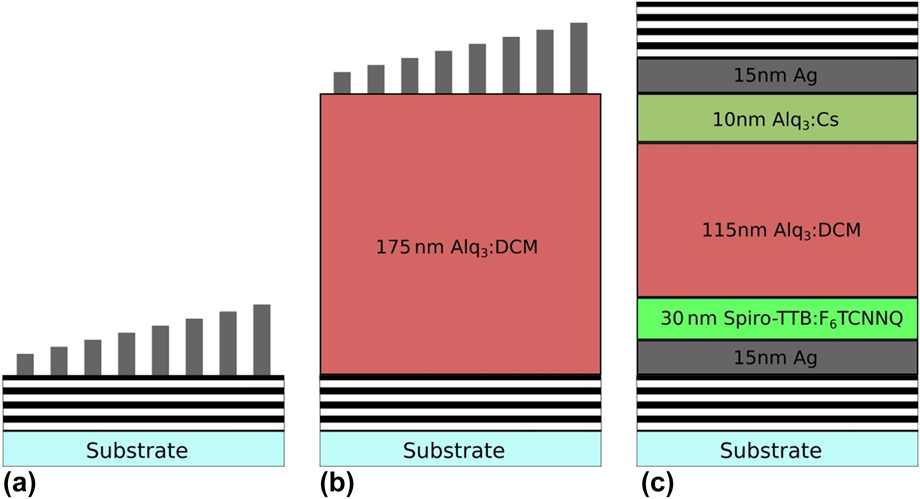
In this paper, we discuss six different sample structures (S1–S6), which are shown in Fig. 1 and are listed in Table I. The OLED (S6) has an untypically thick (115 nm) Alq3:DCM emission layer (EML), which is necessary to fulfill the cavity resonance conditions and to supply enough invertible DCM molecules to reach the optically pumped LT [Reference Brückner, Sudzius, Fröb, Lyssenko and Leo30]. As hole transport layer, a 10-nm Spiro-TTB layer doped with 4 wt% of F6TCNNQ is used. Further, the last 10 nm of the EML is doped with cesium to improve electron injection and electrical stability of the device. The bottom and top contacts consist of 15 nm of silver.
(a) Metals with varying thicknesses on top of a DBR (S1 and S2), (b) metals with varying thicknesses on top of an Alq3:DCM cavity layer (S3, S4, and S5), (c) adjusted pin-OLED structure embedded in an MC (structures are not to scale).

Overview of discussed devices and their compositions.

Samples S1–S5 have varying silver thicknesses on one substrate to compare the quality and to rule out influences due to different processing parameters. To rate the quality of the metal layer compositions, IV characteristics, photoluminescence (PL) spectra, and input–output curves are recorded for all samples. Further, S6 is measured optically and electrically (consecutively and simultaneously) in a µ-PL setup to better understand the influence of the free charge carriers on the functionality of the device, e.g., possible increase in absorption.
Electrical characterization
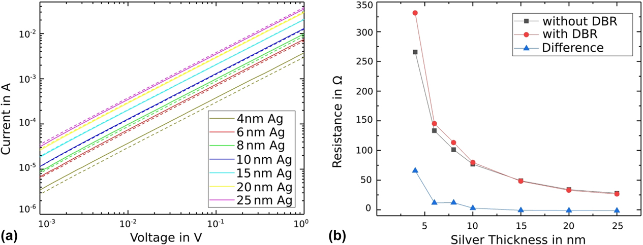
At first, we perform IV measurements for S1–S5. The IV curves of S5 are shown in Fig. 2 (solid lines). The graph is plotted in log–log-scale to show and compare the ohmic behavior over a few orders of magnitude. The measuring tips are placed on either end of the metal stripes and are therefore exactly 2 cm apart. This ensures conductive layers over the width of the whole substrate, which is important for potential devices. All metal stripes are conductive, even the thinnest one, which is only 4 nm thick.
(a) Exemplary IV comparison of structure S5 without (solid lines) and with (dotted lines) top DBR, (b) resistance calculated from (a).
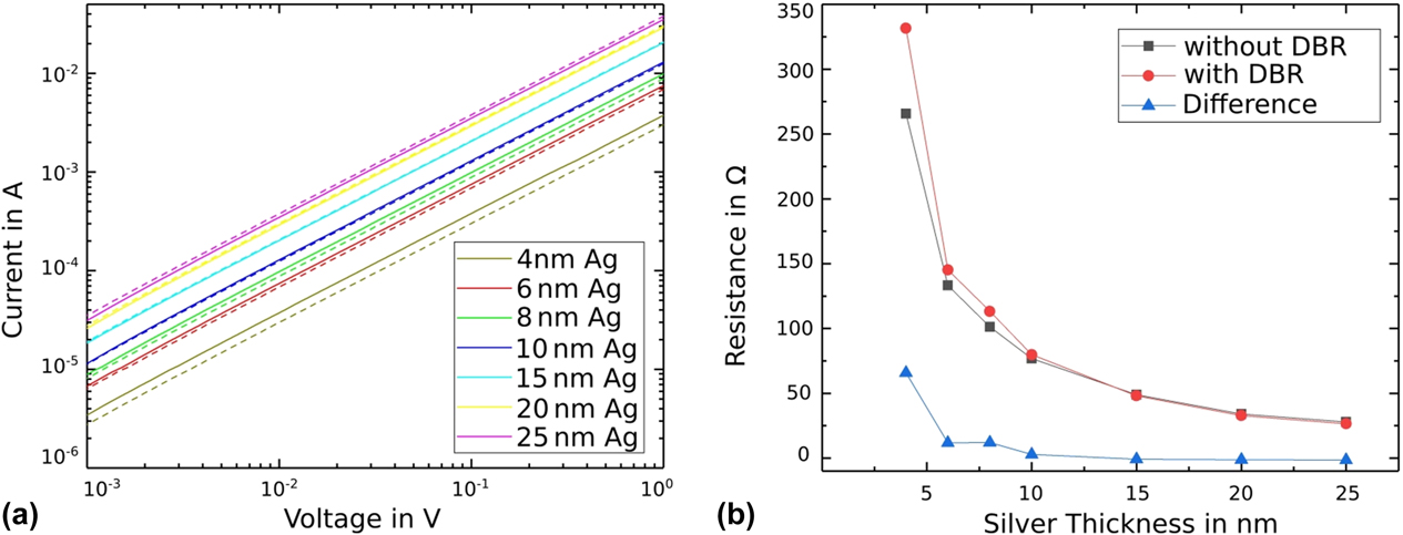
After measuring the IV characteristics, we deposited a DBR on top of the contacts to check the changes in electrical quality. Here, for easier accessibility, the ends of the metal stripes are covered with a metal shadow mask during the deposition of the DBR. As one can see from Fig. 2 (dashed lines), the influence of the deposition of the top DBR is almost negligible; however, the change in the IV characteristics depends on the thickness of the metal. In this case, the thin layers (4, 6, and 8 nm) have a higher resistance, whereas the intermediate layers (10 and 15 nm) remain constant, and the thick layers (20 and 25 nm) have a lower resistance.
We attribute the observed effect to the peculiarities of silver growth. As reported in Ref. Reference Nehm, Schubert, Müller-Messkamp and Leo31, silver layers start to form isles which are growing with time and interconnect at some point, which leads to a closed, conductive layer. The deposition of the top DBR most likely leads to degradation/oxidation of the isles, which effectively reduces the metallic size and, therefore, increases the resistance. The thicker layers already are relatively homogeneous and are probably smoothed due to the top DBR deposition, which leads to a small decrease in resistance.
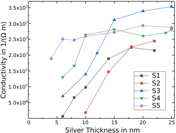
To rate the quality of the contacts, we calculated the conductivities for S1–S5 from the IV characteristics. The conductivity σ is defined as the inverse of the resistivity ρ, which can be calculated with the following formula: ρ = R × h × b/l. Here, R is the electrical resistance, h is the height/thickness, b is the width, and l the length of the metal stripe. We assume a rectangular shape of the contacts, which should be a good approximation. We extract R from the IV characteristics, control/measure the length and width (given by the shadow mask) with a microscope, and use the deposited thicknesses (which are monitored during the deposition by QCMs and spectrally controlled).
The calculated conductivities for S1–S5 are plotted in Fig. 3. The investigated parameters are the position (top/bottom), the seed layer (with and without a 0.5-nm aluminum layer), and the deposition speed. These are the actively influenced parameters. Others, such as the pressure inside the chamber or the quality of the substrate are kept constant, but small variations cannot be ruled out. This shows the complexity of building devices, but also the potential to improve the quality with the perfect deposition parameters.
Calculated conductivities for all structures S1–S5 with varying silver thicknesses.

The first property, which comes into focus, is the minimal silver thickness needed to get a conductive layer. Thinner conductive layers with the same deposition parameters (especially for the bottom contact with seed layer) are possible. However, the conductivity cannot be reproduced at all times; thus, corresponding data points were excluded. Therefore, S2 (circles) needs a minimal silver thickness of 10 nm, whereas for S1 (squares) 6 nm is sufficient. The top contacts can be even thinner and still have higher conductivities of up to one order of magnitude. Both S3 (triangle pointing up) and S4 (triangle pointing down) are conductive at 6 nm. Increasing the deposition rate of silver from 4 to 7 Å/s (rotated squares) leads to conductive layers of only 4-nm silver. Further, the 4-nm-thick contact is not only the thinnest conductive contact, but it already has a relatively high conductivity of approximately 1.9 × 10⁷ (Ω/m). For S1–S5 a stronger increase in conductivity arises for thicker silver layer and saturates for conductivities above 2.5 × 10⁷ (Ω/m). The bottom contact without seed (S1) has a higher conductivity for thinner silver layers, but a lower conductivity for thicker silver layers compared with the bottom contact with seed (S2). The opposite effect occurs for top contacts. Here, the contacts with seed (S4, S5) show higher conductivities for thinner silver stripes and lower conductivities for thicker silver stripes compared with those without seed (S3).
Additionally, the plot shows the importance of the metal composition for very thin layers, because the conductivities are in the same range at approximately 20 nm of silver.
For an organic MC, the total amount of metal inside the cavity layer should be as small as possible. Keeping this in mind, the composition of sample S5 seems to be a good choice for the top contact, because it already provides a very high conductivity [approximately 1.9 × 10⁷ (Ω/m)] with a silver thickness of only a few nm. Further, the composition of the bottom contact should be improved to match the quality of the top contact.
Optical characterization
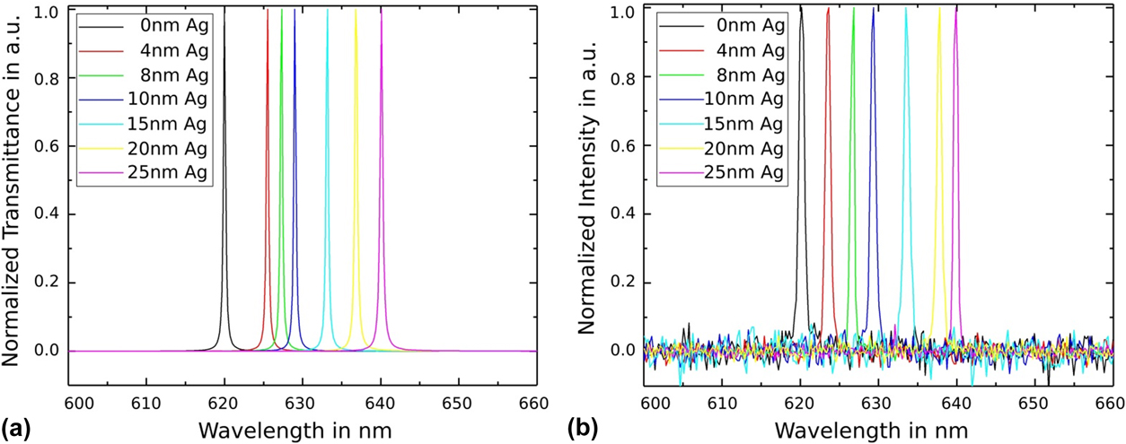
To control the thicknesses of the metal layers with optical precision, we compare the simulated transmittance spectrum [Fig. 4(a)] to the measured PL spectrum [Fig. 4(b)]. The spectral mode positions fit with slight variations. The biggest differences occur for the 8-/20-nm-thick metal layers. Here, the peaks are at 627.32/636.8 nm in the simulation and at 626.85/637.81 nm for the PL measurement. This suggests an actual metal thickness of 7/21.5 nm, respectively. Small deviations in the thickness can occur, especially for high deposition rates. Nevertheless, the biggest difference in thickness is only 1.5 nm and the majority of the stripes fit very well, which shows a high precision in sample preparation.
(a) Simulated transmission spectra and (b) experimentally measured PL spectra for different thicknesses of the intracavity contact.

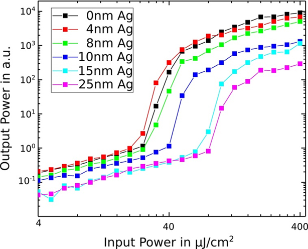
We have measured input–output characteristics for S5 with a top DBR to check optical and lasing characteristics of our structures with build-in metal intracavity contacts. Figure 5 shows emission intensity as a function of pump power for every metal stripe individually pumped by a fs laser system. The LT was reached in all cases and varied from ≈20 to ≈80 µJ/cm2 depending on the thickness of the intracavity metal contact. The lowest LT was achieved in a metal-free area and is very close to a typical threshold value for our metal-free planar organic Alq3:DCM microcavities [Reference Koschorreck, Gehlhaar, Lyssenko, Swoboda, Hoffmann and Leo10, Reference Meister, Brückner, Sudzius, Fröb and Leo20]. However, the threshold for the 4-nm-thick silver layer is nearly the same as for the purely organic region. We consider this as a very good result due to a relatively high electrical conductivity of approximately 1.9 × 10⁷ (Ω/m), which is promising for electrically pumped structures.
Input–output curves of structure S5 with varying silver thicknesses. The LT for the metal free area is around 20 µJ/cm2. For the metal thicknesses above 10 nm, the LT increases up to 80 µJ/cm2. The increase in LT for metal thicknesses below 8 nm is very small.

Below LT, the emission intensity is systematically reduced by one order of magnitude with the thickness of the intracavity contact, due to different kinds of optical losses in the metal. This reduction, however, gets much more pronounced above LT (≈1.5 orders of magnitude, see Fig. 5) and should rather be attributed to laser characteristics than only the linear energy dissipation on the metal contacts. We attribute the observed enhancement of the emission losses to the reduced overall optical quality of the resonator (quality factor Q) and, therefore, to the smaller mode volumes (and consequently lasing volumes) above LT as more metal is inserted into the cavity. However, the reduction in emission intensity above LT (and also increase in LT) is very small for the intracavity silver contacts up to a thickness of 8 nm.
Simultaneous optical and electrical excitation
Realizing a highly efficient top contact leaves two tasks for a better understanding of the system and the possibility of defining the electrical LT. The first aim is to optimize the bottom contact, ideally, to match the quality of the top contact. The second task is to identify potential influences on the device performance caused by high densities of charge carriers, especially close to the threshold. An electronic absorption for wavelengths in the visible regime is not expected. This assumption originates in the concentration of charge carriers being orders of magnitude lower than the molecular density. Nevertheless, additional charges have an influence on the vibronic and polariton states.
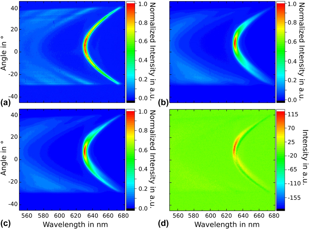
To clarify differences and similarities between various pumping mechanisms, we have measured and analyzed far-field images from a hybrid OLED–MC device [Fig. 1(c)] under pure electrical, pure optical, and hybrid pumping which means using both pumping techniques simultaneously. In all cases, the structures are pumped below LT to prevent degradation and to allow repeated measurements. The current densities are limited to the maximum of 10 A/cm2, which is at least two orders of magnitude lower than the expected LT.
Figure 6 shows far-field images where the structure is (a) optically pumped with a 405-nm cw laser diode, (b) electrically pumped (34 V, 26 µA, 100 × 100 µm2, j = 0.26 A/cm2), and (c) optically (same intensity as in a) and electrically (same intensity as in b) pumped at the same time. Figure 6(d) shows the measurement (c) with the results of (a) and (b) subtracted.
Investigation of a hybrid OLED–MC device [Fig. 1(c)]. (a) Optically pumped with a 405-nm cw laser diode, (b) electrically pumped with a current density of j = 0.26 A/cm2, (c) simultaneous optical and electrical excitation [same intensities as in (a) and (b)], (d) measurement (c) with the results of (a) and (b) subtracted.

Importantly, the excited areas differ for optical and electrical excitation. The diameter of the laser beam was approximately 7 µm, which leads to a circular pump area of 38.5 µm2, whereas the active area of the OLED is defined by the width of the contacts, which in this case is 100 × 100 µm2 (the laser beam is positioned in the center of the electrical active area). Therefore, the electrically excited area is approximately 260 times larger than the active area under optical excitation. This leads to a somewhat wider angular intensity distribution for optical excitation as presented in Fig. 6(a), due to more distinct light diffraction. In contrast, the maximum intensity of the mode is relatively constant for detection angles of ±10°, whereas it is only ±5° for the electrically pumped structure. Except from the intensity distribution, the parabolic shape of the modes is similar, which leads to approximately the same Q-factors of 300.
For combined excitation [Fig. 6(c)], with the same intensities, the far-field image seems to be the sum of Figs. 6(a) and 6(b). It shows higher intensities for smaller angles (due to an overall higher electrical intensity), but the optical parabola branch for angles above ±10° can be seen. Further, the image shows a small shift in the optical axis for the electrical and optical excitation, which in this case is useful to distinguish between both parts.
The highest intensity for all three images is in the apex of the parabola. Further, if the maxima of optical and electrical single excitation are added up it gives the maximum intensity of the simultaneous excitation. This is a promising result, because at least for electrical pump intensities below the LT, there is no significant additional absorption caused by the injected charge carriers.
Finally, Fig. 6(d) clearly shows that combined optical and electrical pumping of the structure does not equal a simple superposition of two separate and independent pumping processes. Instead, nonlinear interaction between them takes place and has to be considered. The plot still shows a mode with features of both the electrical and optical modes. This identification is possible, due to the small tilt of the optical axes mentioned previously. The features belonging to the optical excitation show negative values, whereas the features of the electrical excitation show positive values. As a conclusion, the optical excitation increases the functionality of the electrical process at the cost of a reduced optical efficiency. We tested different excitation energies (same order of magnitude to prevent degradation) and observed the same effect.
There are several explanations we are currently investigating to better understand this effect.
One of the reasons for such a behavior could be the partial absorption of the pump beam [either by the metal(s) or the cc] which could increase the cc injection or the energy of the cc. Both options can increase the amount of radiatively recombining cc.
The second explanation is an unbalance for the cc in this adjusted pin-OLED structure. The optical excitation shifts the recombination zone toward the center of the cavity layer where the electric field enhancement has its maximum. Therefore, the electrical functionality is increased without influencing the amount of cc.
The observed mutual coupling between two pumping regimes could also be related to the long-term accumulation of triplet states. Continues-wave optical pump could further promote triplets conversion back to the singlet states. Further fundamental research is necessary and in progress to fully understand and to answer these questions.
In conclusion, we improved the functionality and increased the understanding of an electrically active structure in an MC. Especially, the realization of a very thin (4 nm), high-quality metal contact is promising. The properties of these metal contacts are also of interest for other applications where absorption and reflection of metals is harmful, but a high conductivity is essential. In our first experiments with simultaneous optical and electrical excitation, we found the influence of the cc, especially for electrical excitation, to be negligible. Moreover, additional optical pumping might increase electrical efficiency. This surely has to be tested for higher charge carrier concentrations, which was not yet possible. All in all, these results are a good basis to build improved devices which allows to get closer to the electrical LT and supply insights in areas which could potentially be further optimized.
Experiments and results
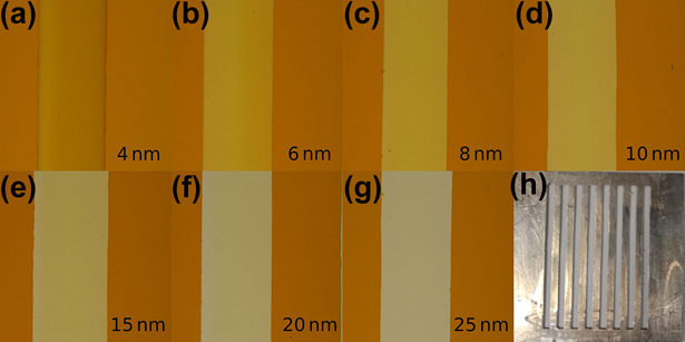
The macroscopic appearance of S1–S5 is checked using a Nikon Eclipse LV100ND microscope (Nikon Industrial Metrology GmbH, Alzenau, Germany). Figure 7 shows images from S5 for all investigated silver thicknesses (4, 6, 8, 10, 15, 20, and 25 nm). A difference in transmission of the metal layers is clearly visible. The last image [Fig. 7(h)] is a picture of the metal shadow mask used to deposit metal stripes with different thicknesses on one substrate.
(a)–(g) Micrograph of S5. Silver thicknesses are indicated directly in the pictures. (h) Metal shadow mask, which was used during the thermal evaporation of the metals. The width of the stripes is 1 mm and the length is 2 cm.

Acknowledgment
The authors gratefully acknowledge support by the German Research Foundation (DFG) with the DFG projects Tailored Disorder SPP1839, Nos. LE 747/47-1 and 747/55-1 as well as the Cluster of Excellence Center for Advancing Electronics Dresden.