1 Introduction
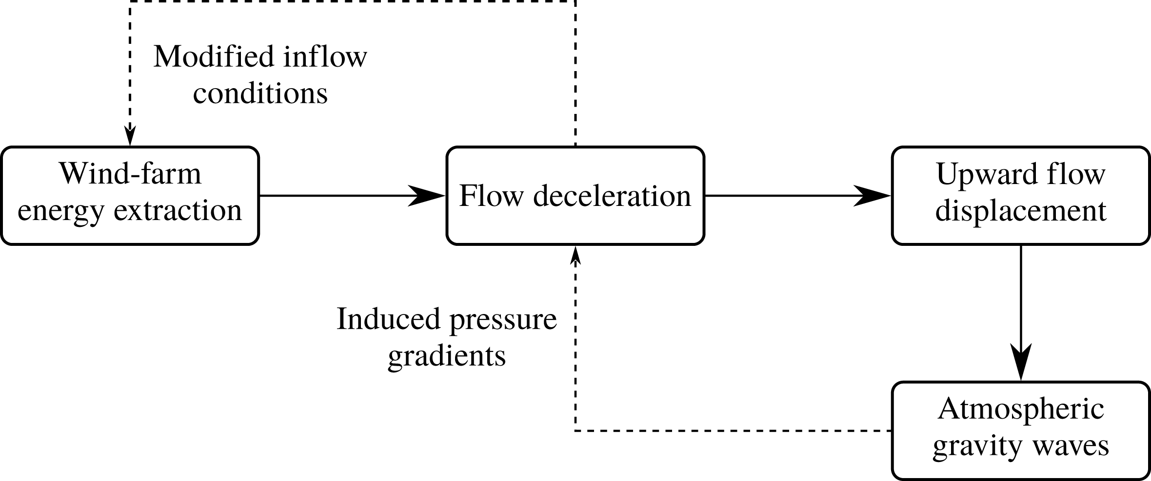
Previous research on the interaction between wind farms and the atmospheric boundary layer (ABL) has found that in some situations wind farms excite atmospheric gravity waves in the free atmosphere and on the interface between the boundary layer and the free atmosphere (see e.g. Fitch et al. Reference Fitch, Olson, Lundquist, Dudhia, Gupta, Michalakes and Barstad2012; Volker Reference Volker2014; Allaerts & Meyers Reference Allaerts and Meyers2017; Wu & Porté-Agel Reference Wu and Porté-Agel2017). Wind-farm gravity waves are triggered by the upward displacement of the boundary layer due to flow blockage inside the farm. The waves excited by the wind farm induce significant changes in the regional pressure field around the farm, which may modify the wind conditions several kilometres upstream of the farm. This non-local effect induces a feedback mechanism that can lead to reduced wind-farm energy extraction (see figure 1). The goal of the current study is to assess the sensitivity of gravity-wave excitation to the atmospheric state and the wind-farm configuration. Moreover, we investigate the impact of gravity waves on upstream wind conditions and the resulting feedback on wind-farm energy extraction in order to identify the physical regimes in which gravity-wave-induced power loss is significant.
Generation and feedback mechanism of wind-farm gravity waves.

The existence of wind-farm-induced gravity waves was first hypothesised by Smith (Reference Smith2010). Based on a linear quasi-analytical model of the atmospheric response to wind-farm drag, he found that gravity-wave excitation is governed by three non-dimensional parameters: a Froude number, a stratification parameter and a frictional recovery parameter. However, Smith’s simple theory only describes how gravity waves are generated and how they affect the wind conditions, but does not account for gravity-wave feedback on wind-farm energy extraction. More recently, gravity waves were observed in wind-farm studies based on numerical simulations with either the Weather Research and Forecasting (WRF) model (Fitch et al. Reference Fitch, Olson, Lundquist, Dudhia, Gupta, Michalakes and Barstad2012; Fitch, Lundquist & Olson Reference Fitch, Lundquist and Olson2013; Volker Reference Volker2014) or large-eddy simulation (LES) models (Allaerts & Meyers Reference Allaerts and Meyers2017, Reference Allaerts and Meyers2018; Wu & Porté-Agel Reference Wu and Porté-Agel2017). While these studies provided essential insights based on detailed flow information, they only performed a few simulations for very specific flow conditions and wind-farm configurations due to the high computational cost of the flow models. In this paper, we conduct a more extensive study of all relevant parameters. To this end, we develop and validate a new fast boundary-layer model based on a three-layer representation of the atmosphere.
The modelling approach followed in this paper is similar to the theory for interacting gravity waves and boundary layers developed by Smith, Jiang & Doyle (Reference Smith, Jiang and Doyle2006) and Smith (Reference Smith2007, Reference Smith2010). However, the three-layer model presented here aims to include additional physical aspects that are not considered in the simple wind-farm gravity-wave theory of Smith (Reference Smith2010). First, in order to investigate the feedback of gravity waves to wind-farm energy extraction, a two-way coupling between the boundary-layer model and the wind-farm model is established (see e.g. the simple model developed by Allaerts & Meyers Reference Allaerts and Meyers2018). Second, Smith (Reference Smith2010) assumes that ‘the turbine drag has been mixed homogeneously between turbines and vertically up to the top of the boundary-layer’. In reality, the turbine drag is only felt within an internal boundary layer that grows slowly above the farm (see e.g. Chamorro & Porté-Agel Reference Chamorro and Porté-Agel2011; Wu & Porté-Agel Reference Wu and Porté-Agel2013; Allaerts & Meyers Reference Allaerts and Meyers2017). In order to relax the vertical mixing assumption, the boundary layer is divided into two regions and turbine forces are only added in the lower region. Moreover, by representing the boundary layer with two layers, the model can also account for some large-scale effects related to vertical wind shear and wind veer, like the wind-farm wake deflection observed by van der Laan & Sørensen (Reference van der Laan and Sørensen2017).
The paper is further organised as follows. The three-layer model is introduced in § 2 and validated against LES data in § 3. Subsequently, we analyse the model characteristics and the induced flow physics in § 4. The sensitivity of wind-farm gravity waves to the atmospheric state and the wind-farm configuration is explored in § 5, and conclusions are given in § 6.
2 Model description
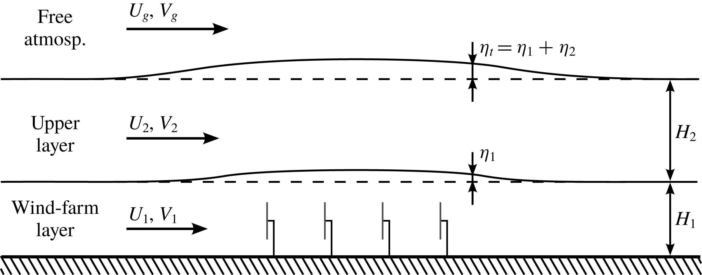
The idea of the three-layer model is to divide the vertical structure of the atmosphere into three parts (see figure 2). The lowest layer (called the wind-farm layer) corresponds to the wind-farm region of the atmospheric boundary layer within which the wind-turbine drag forces are felt directly. The second layer (called the upper layer) starts above the wind turbines and extends up to the capping inversion, and this layer is only indirectly affected by the wind farm through vertical turbulent transport of momentum. The free atmosphere above the inversion layer constitutes the third layer of the model. The flow in the two layers comprising the ABL is simulated explicitly, while the third layer provides a relationship between the pressure and the vertical displacement at the top of the boundary layer. The interfaces between the wind-farm layer, the upper layer and the free atmosphere are thereby treated as pliant surfaces, i.e. there is no mean mass flux across these surfaces, and horizontal flow divergence or convergence results in variations of the depth of the respective layers.
Conceptual sketch of the three-layer model.

First, we derive a general set of equations describing the depth-averaged flow behaviour in a layer of fluid from the incompressible Navier–Stokes equations in § 2.1. Subsequently, we formulate the linearised equations for the wind-farm layer and upper layer of the three-layer model in § 2.2 and elaborate the coupling with the free atmosphere by means of gravity waves in § 2.3. In § 2.4, we explain how to determine the background state variables based on observational, numerical or theoretical vertical profiles. The wind-farm drag force is discussed in § 2.5.
2.1 General depth-averaged flow equations
We start from the incompressible, three-dimensional Reynolds-averaged Navier–Stokes equations for the atmospheric boundary layer (see e.g. Stull Reference Stull1988):
 $$\begin{eqnarray}\displaystyle & \unicode[STIX]{x1D735}\boldsymbol{\cdot }\overline{\boldsymbol{u}}=0, & \displaystyle\end{eqnarray}$$
 $$\begin{eqnarray}\displaystyle & \displaystyle \unicode[STIX]{x2202}_{t}\overline{\boldsymbol{u}}+\overline{\boldsymbol{u}}\boldsymbol{\cdot }\unicode[STIX]{x1D735}\overline{\boldsymbol{u}}=-\frac{1}{\unicode[STIX]{x1D70C}_{0}}\unicode[STIX]{x1D735}\overline{p}+2\unicode[STIX]{x1D734}\times (\boldsymbol{U}_{g}-\overline{\boldsymbol{u}})+\unicode[STIX]{x1D735}\boldsymbol{\cdot }\unicode[STIX]{x1D749}+\frac{\overline{\unicode[STIX]{x1D703}}-\unicode[STIX]{x1D703}_{0}}{\unicode[STIX]{x1D703}_{0}}\boldsymbol{g}, & \displaystyle\end{eqnarray}$$
 $$\begin{eqnarray}\displaystyle & \unicode[STIX]{x2202}_{t}\overline{\unicode[STIX]{x1D703}}+\overline{\boldsymbol{u}}\boldsymbol{\cdot }\unicode[STIX]{x1D735}\overline{\unicode[STIX]{x1D703}}=\unicode[STIX]{x1D735}\boldsymbol{\cdot }\boldsymbol{q}. & \displaystyle\end{eqnarray}$$
The variables
 $\overline{\boldsymbol{u}}=(\overline{u},\overline{v},\overline{w})$
and
 $\overline{\unicode[STIX]{x1D703}}$
denote the velocity and potential temperature, respectively, and the bar indicates ensemble averaging. The Coriolis force is expressed using the angular velocity of the Earth
 $\unicode[STIX]{x1D734}=(0,0,\unicode[STIX]{x1D6FA}\sin \unicode[STIX]{x1D719})$
with
 $\unicode[STIX]{x1D719}$
the latitude (we neglect the horizontal components of
 $\unicode[STIX]{x1D734}$
, which usually have a small impact (see e.g. Gill Reference Gill1982; Wyngaard Reference Wyngaard2010)). Further,
 $\unicode[STIX]{x1D70C}_{0}$
is the density of the adiabatic base state and is assumed to be constant (Bousinesq approximation), and
 $\overline{p}$
denotes the pressure excluding contributions from large-scale pressure gradients, which are included through the geostrophic balance as
 $2\unicode[STIX]{x1D734}\times \boldsymbol{U}_{g}$
with
 $\boldsymbol{U}_{g}=(U_{g},V_{g},0)$
the geostrophic wind velocity. The Reynolds stress tensor is denoted as
 $\unicode[STIX]{x1D749}=-\overline{\boldsymbol{u}^{\prime }\boldsymbol{u}^{\prime }}$
with the primes indicating turbulent fluctuations, and
 $\boldsymbol{q}=-\overline{\boldsymbol{u}^{\prime }\unicode[STIX]{x1D703}^{\prime }}$
corresponds to the turbulent heat flux. The last term in (2.2) represents the buoyancy force in the Boussinesq approximation, with
 $\boldsymbol{g}=(0,0,g)$
the gravitational acceleration and
 $\unicode[STIX]{x1D703}_{0}$
a reference potential temperature.
Consider now a layer of fluid between two pliant surfaces
 $z_{a}(x,y,t)$
and
 $z_{b}(x,y,t)$
for which (Baines Reference Baines1995)
 $$\begin{eqnarray}\begin{array}{@{}c@{}}\overline{w}(z_{a})=\unicode[STIX]{x2202}_{t}z_{a}+\overline{u}(z_{a})\unicode[STIX]{x2202}_{x}z_{a}+\overline{v}(z_{a})\unicode[STIX]{x2202}_{y}z_{a},\\ \overline{w}(z_{b})=\unicode[STIX]{x2202}_{t}z_{b}+\overline{u}(z_{b})\unicode[STIX]{x2202}_{x}z_{b}+\overline{v}(z_{b})\unicode[STIX]{x2202}_{y}z_{b}.\end{array}\end{eqnarray}$$
The depth-averaged flow equations for this layer are found by vertically integrating the Navier–Stokes equations between
 $z_{a}$
and
 $z_{b}$
and dividing by the height of the layer
 $h=z_{b}-z_{a}$
. We use the following notation:
 $$\begin{eqnarray}\langle \unicode[STIX]{x1D719}\rangle =\frac{1}{h}\int _{z_{a}}^{z_{b}}\unicode[STIX]{x1D719}\,\text{d}z\quad \text{and}\quad \unicode[STIX]{x1D719}=\langle \unicode[STIX]{x1D719}\rangle +\unicode[STIX]{x1D719}^{\prime \prime }\end{eqnarray}$$
so that
 $$\begin{eqnarray}\langle \unicode[STIX]{x1D719}^{\prime \prime }\rangle =0\quad \text{and}\quad \langle \unicode[STIX]{x1D719}\unicode[STIX]{x1D719}\rangle =\langle \unicode[STIX]{x1D719}\rangle \langle \unicode[STIX]{x1D719}\rangle +\langle \unicode[STIX]{x1D719}^{\prime \prime }\unicode[STIX]{x1D719}^{\prime \prime }\rangle .\end{eqnarray}$$
The depth-averaged continuity equation is found by integrating (2.1) between
 $z_{a}(x,y,t)$
and
 $z_{b}(x,y,t)$
and subsequently changing the order of integration and differentiation using Leibniz’s differentiation rules. Exploiting the fact that
 $z_{a}$
and
 $z_{b}$
represent pliant surfaces obeying (2.4) reduces the depth-averaged continuity equation to
 $$\begin{eqnarray}\unicode[STIX]{x2202}_{t}h+\unicode[STIX]{x1D735}_{h}\boldsymbol{\cdot }h\langle \overline{\boldsymbol{u}}_{h}\rangle =0,\end{eqnarray}$$
where
 $\overline{\boldsymbol{u}}_{h}=(\overline{u},\overline{v})$
is the two-dimensional horizontal velocity vector and
 $\unicode[STIX]{x1D735}_{h}=(\unicode[STIX]{x2202}_{x},\unicode[STIX]{x2202}_{y})$
is the two-dimensional horizontal del operator.
The depth-averaged momentum equation is derived in a similar way from the horizontal components of (2.2). The convective terms are thereby transformed using (2.4), (2.6) and (2.7). The result can be written as
 $$\begin{eqnarray}\displaystyle \unicode[STIX]{x2202}_{t}\langle \overline{\boldsymbol{u}}_{h}\rangle +\langle \overline{\boldsymbol{u}}_{h}\rangle \boldsymbol{\cdot }\unicode[STIX]{x1D735}_{h}\langle \overline{\boldsymbol{u}}_{h}\rangle & = & \displaystyle -\frac{1}{\unicode[STIX]{x1D70C}_{0}}\unicode[STIX]{x1D735}_{h}\langle \overline{p}\rangle +f_{c}\unicode[STIX]{x1D645}\boldsymbol{\cdot }(\boldsymbol{U}_{g,h}-\langle \overline{\boldsymbol{u}}_{h}\rangle )\nonumber\\ \displaystyle & & \displaystyle +\,\frac{\unicode[STIX]{x1D749}_{h3}|_{z_{a}}^{z_{b}}}{h}+\unicode[STIX]{x1D735}_{h}\boldsymbol{\cdot }\langle \unicode[STIX]{x1D749}_{hh}\rangle -\frac{1}{h}\unicode[STIX]{x1D735}_{h}\boldsymbol{\cdot }h\langle \overline{\boldsymbol{u}}_{h}^{\prime \prime }\overline{\boldsymbol{u}}_{h}^{\prime \prime }\rangle +\frac{\mathscr{R}}{h},\end{eqnarray}$$
with
 $$\begin{eqnarray}\displaystyle \mathscr{R} & = & \displaystyle \frac{1}{\unicode[STIX]{x1D70C}_{0}}[\overline{p}(z_{b})-\langle \overline{p}\rangle ]\unicode[STIX]{x1D735}_{h}z_{b}-\frac{1}{\unicode[STIX]{x1D70C}_{0}}[\overline{p}(z_{a})-\langle \overline{p}\rangle ]\unicode[STIX]{x1D735}_{h}z_{a}\nonumber\\ \displaystyle & & \displaystyle -\,[\unicode[STIX]{x1D749}_{hh}(z_{b})-\langle \unicode[STIX]{x1D749}_{hh}\rangle ]\boldsymbol{\cdot }\unicode[STIX]{x1D735}_{h}z_{b}+[\unicode[STIX]{x1D749}_{hh}(z_{a})-\langle \unicode[STIX]{x1D749}_{hh}\rangle ]\boldsymbol{\cdot }\unicode[STIX]{x1D735}_{h}z_{a},\end{eqnarray}$$
where
 $\unicode[STIX]{x1D749}_{h3}=-\overline{\boldsymbol{u}_{h}^{\prime }w^{\prime }}$
and
 $\unicode[STIX]{x1D749}_{hh}=-\overline{\boldsymbol{u}_{h}^{\prime }\boldsymbol{u}_{h}^{\prime }}$
. The horizontal component of the Coriolis force has been denoted using the Coriolis parameter
 $f_{c}=2\unicode[STIX]{x1D6FA}\sin \unicode[STIX]{x1D719}$
and the two-dimensional rotation dyadic
 $\unicode[STIX]{x1D645}=\boldsymbol{e}_{1}\boldsymbol{e}_{2}-\boldsymbol{e}_{2}\boldsymbol{e}_{1}$
(with
 $\boldsymbol{e}_{1}$
and
 $\boldsymbol{e}_{2}$
two-dimensional unit vectors in the
 $x$
and
 $y$
directions, respectively), and
 $\boldsymbol{U}_{g,h}$
represents the horizontal component of the geostrophic wind velocity.
The last four terms in (2.8) depend on turbulent quantities or vertical profiles and need to be modelled. First,
 $\unicode[STIX]{x1D749}_{h3}|_{z_{a}}^{z_{b}}$
is the vertical turbulent shear stress and represents the momentum flux through the boundary surfaces. We take this term proportional to the product of the mean horizontal wind speed and the mean horizontal wind vector relative to the adjacent layer (see e.g. Wyngaard Reference Wyngaard2010), i.e.
 $$\begin{eqnarray}\unicode[STIX]{x1D749}_{h3}\sim \Vert \unicode[STIX]{x0394}\langle \overline{\boldsymbol{u}}_{h}\rangle \Vert \unicode[STIX]{x0394}\langle \overline{\boldsymbol{u}}_{h}\rangle ,\end{eqnarray}$$
where
 $\unicode[STIX]{x0394}\langle \overline{\boldsymbol{u}}_{h}\rangle =\langle \overline{\boldsymbol{u}}_{h}\rangle _{+}-\langle \overline{\boldsymbol{u}}_{h}\rangle _{-}$
with
 $\langle \overline{\boldsymbol{u}}_{h}\rangle _{+}$
the velocity above the pliant surface and
 $\langle \overline{\boldsymbol{u}}_{h}\rangle _{-}$
below. When the adjacent layer is a solid boundary, we simply set its velocity to zero. Next,
 $\langle \unicode[STIX]{x1D749}_{hh}\rangle$
represents horizontal diffusion by means of turbulence, and we model this term as
 $$\begin{eqnarray}\langle \unicode[STIX]{x1D749}_{hh}\rangle =\unicode[STIX]{x1D708}_{t}\unicode[STIX]{x1D735}_{h}\langle \overline{\boldsymbol{u}}_{h}\rangle ,\end{eqnarray}$$
with
 $\unicode[STIX]{x1D708}_{t}$
a depth-averaged turbulent viscosity. Finally, the term
 $\langle \overline{\boldsymbol{u}}_{h}^{\prime \prime }\overline{\boldsymbol{u}}_{h}^{\prime \prime }\rangle$
represents the redistribution of momentum due to the vertical variation of the horizontal velocity (sometimes called Taylor-shear dispersion), and
 $\mathscr{R}$
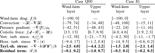
is a residual term related to vertical variations in pressure and Reynolds stresses. As shown in § A.1, both of these terms are generally small compared to the dominant terms in the momentum equation (i.e. less than 4.4 % and 1 %, respectively), and they are neglected in this study.
The depth-averaged continuity equation (2.7) and horizontal momentum equation (2.8) do not depend explicitly on the vertical velocity
 $\langle \overline{w}\rangle$
or potential temperature
 $\langle \overline{\unicode[STIX]{x1D703}}\rangle$
. These variables only affect the horizontal depth-averaged flow implicitly through their impact on turbulent quantities and deviations from the vertical mean. Since the various effects of turbulence and vertical fluctuations are either modelled or neglected, the depth-averaged equations for vertical momentum and potential temperature need not be considered explicitly. The layer of fluid is fully described by the evolution of
 $h$
and
 $\langle \overline{\boldsymbol{u}}_{h}\rangle$
, and the pressure in the layer follows from the boundary conditions. In the remainder of this study, the subscript
 $h$
is omitted for simplicity and all vector notations imply two-dimensional vectors and operators in the horizontal plane.
2.2 Linearised equations for steady-state flow conditions
The evolution of the depth-averaged velocity and the height of both the wind-farm layer (
 $\langle \overline{\boldsymbol{u}}\rangle _{1},h_{1}$
) and the upper layer (
 $\langle \overline{\boldsymbol{u}}\rangle _{2},h_{2}$
) are described by the general depth-averaged flow equations (2.7) and (2.8). In the current study, we only consider steady-state conditions and assume that momentum entrainment at the top of the upper layer is suppressed by the capping inversion (Taylor & Sarkar Reference Taylor and Sarkar2008). Moreover, given the narrow vertical scale of the boundary layer relative to the horizontal scale of wind farms and gravity waves, we can make the boundary-layer approximation and presume that the pressure does not vary with height in the boundary layer such that
 $\langle \overline{p}\rangle _{1}=\langle \overline{p}\rangle _{2}=p$
(analysis of LES data in § A.1 shows that the difference in pressure is usually smaller than 12 %). The governing equations can then be written as
 $$\begin{eqnarray}\displaystyle & \displaystyle \langle \overline{\boldsymbol{u}}\rangle _{1}\boldsymbol{\cdot }\unicode[STIX]{x1D735}\langle \overline{\boldsymbol{u}}\rangle _{1}=-\frac{1}{\unicode[STIX]{x1D70C}_{0}}\unicode[STIX]{x1D735}p+f_{c}\unicode[STIX]{x1D645}\boldsymbol{\cdot }(\boldsymbol{U}_{g}-\langle \overline{\boldsymbol{u}}\rangle _{1})+\frac{\unicode[STIX]{x1D749}_{3,1}-\unicode[STIX]{x1D749}_{3,0}}{h_{1}}+\unicode[STIX]{x1D708}_{t,1}\unicode[STIX]{x1D6FB}^{2}\langle \overline{\boldsymbol{u}}\rangle _{1}+\frac{\boldsymbol{f}}{h_{1}},\qquad & \displaystyle\end{eqnarray}$$
 $$\begin{eqnarray}\displaystyle & \displaystyle \langle \overline{\boldsymbol{u}}\rangle _{2}\boldsymbol{\cdot }\unicode[STIX]{x1D735}\langle \overline{\boldsymbol{u}}\rangle _{2}=-\frac{1}{\unicode[STIX]{x1D70C}_{0}}\unicode[STIX]{x1D735}p+f_{c}\unicode[STIX]{x1D645}\boldsymbol{\cdot }(\boldsymbol{U}_{g}-\langle \overline{\boldsymbol{u}}\rangle _{2})-\frac{\unicode[STIX]{x1D749}_{3,1}}{h_{2}}+\unicode[STIX]{x1D708}_{t,2}\unicode[STIX]{x1D6FB}^{2}\langle \overline{\boldsymbol{u}}\rangle _{2},\qquad & \displaystyle\end{eqnarray}$$
and
 $$\begin{eqnarray}\unicode[STIX]{x1D735}\boldsymbol{\cdot }h_{1}\langle \overline{\boldsymbol{u}}\rangle _{1}=0,\quad \unicode[STIX]{x1D735}\boldsymbol{\cdot }h_{2}\langle \overline{\boldsymbol{u}}\rangle _{2}=0.\end{eqnarray}$$
The term
 $\boldsymbol{f}$
represents an external force (e.g. wind-farm drag) and the friction terms at the ground and at the interface between the two layers are expressed by (see (2.10))
 $$\begin{eqnarray}\displaystyle & \unicode[STIX]{x1D749}_{3,0}=C\Vert \langle \overline{\boldsymbol{u}}\rangle _{1}\Vert \langle \overline{\boldsymbol{u}}\rangle _{1}, & \displaystyle\end{eqnarray}$$
 $$\begin{eqnarray}\displaystyle & \unicode[STIX]{x1D749}_{3,1}=D\Vert \unicode[STIX]{x0394}\langle \overline{\boldsymbol{u}}\rangle \Vert \unicode[STIX]{x0394}\langle \overline{\boldsymbol{u}}\rangle , & \displaystyle\end{eqnarray}$$
with
 $\unicode[STIX]{x0394}\langle \overline{\boldsymbol{u}}\rangle =\langle \overline{\boldsymbol{u}}\rangle _{2}-\langle \overline{\boldsymbol{u}}\rangle _{1}$
. Note that the friction coefficients
 $C$
and
 $D$
are constant and cannot account for drastic changes in ambient turbulent intensity due to, e.g., turbine wake flow. An assessment of this approximation can be found in § A.2.
We now consider small perturbations
 $(\boldsymbol{u}_{1},\unicode[STIX]{x1D702}_{1})$
and
 $(\boldsymbol{u}_{2},\unicode[STIX]{x1D702}_{2})$
to a horizontally invariant reference state
 $(\boldsymbol{U}_{1},H_{1})$
and
 $(\boldsymbol{U}_{2},H_{2})$
in response to the drag force exerted by a wind farm. The governing equations (2.12)–(2.14) can then be linearised with respect to the background state variables. With the geostrophic wind (i.e. the mean pressure gradient) balancing the vertical momentum transport and the Coriolis force in the unperturbed state, we find
 $$\begin{eqnarray}\displaystyle & \displaystyle \boldsymbol{U}_{1}\boldsymbol{\cdot }\unicode[STIX]{x1D735}\boldsymbol{u}_{1}+\frac{1}{\unicode[STIX]{x1D70C}_{0}}\unicode[STIX]{x1D735}p=-f_{c}\unicode[STIX]{x1D645}\boldsymbol{\cdot }\boldsymbol{u}_{1}+\unicode[STIX]{x1D708}_{t,1}\unicode[STIX]{x1D6FB}^{2}\boldsymbol{u}_{1}+\frac{\unicode[STIX]{x1D63F}^{\prime }}{H_{1}}\boldsymbol{\cdot }\unicode[STIX]{x0394}\boldsymbol{u}-\frac{\unicode[STIX]{x1D63E}^{\prime }}{H_{1}}\boldsymbol{\cdot }\boldsymbol{u}_{1}+\frac{\boldsymbol{f}^{(0)}+\,\boldsymbol{f}^{(1)}}{H_{1}},\qquad & \displaystyle\end{eqnarray}$$
 $$\begin{eqnarray}\displaystyle & \displaystyle \boldsymbol{U}_{2}\boldsymbol{\cdot }\unicode[STIX]{x1D735}\boldsymbol{u}_{2}+\frac{1}{\unicode[STIX]{x1D70C}_{0}}\unicode[STIX]{x1D735}p=-f_{c}\unicode[STIX]{x1D645}\boldsymbol{\cdot }\boldsymbol{u}_{2}+\unicode[STIX]{x1D708}_{t,2}\unicode[STIX]{x1D6FB}^{2}\boldsymbol{u}_{2}-\frac{\unicode[STIX]{x1D63F}^{\prime }}{H_{2}}\boldsymbol{\cdot }\unicode[STIX]{x0394}\boldsymbol{u},\qquad & \displaystyle\end{eqnarray}$$
 $$\begin{eqnarray}\displaystyle & \boldsymbol{U}_{1}\boldsymbol{\cdot }\unicode[STIX]{x1D735}\unicode[STIX]{x1D702}_{1}+H_{1}\unicode[STIX]{x1D735}\boldsymbol{\cdot }\boldsymbol{u}_{1}=0,\qquad & \displaystyle\end{eqnarray}$$
 $$\begin{eqnarray}\displaystyle & \boldsymbol{U}_{2}\boldsymbol{\cdot }\unicode[STIX]{x1D735}\unicode[STIX]{x1D702}_{2}+H_{2}\unicode[STIX]{x1D735}\boldsymbol{\cdot }\boldsymbol{u}_{2}=0,\qquad & \displaystyle\end{eqnarray}$$
with
 $\unicode[STIX]{x0394}\boldsymbol{u}=\boldsymbol{u}_{2}-\boldsymbol{u}_{1}$
. The matrices
 $\unicode[STIX]{x1D63E}^{\prime }$
and
 $\unicode[STIX]{x1D63F}^{\prime }$
describe the perturbation of the friction at the ground and at the interface between both layers, respectively, and they are given by
 $$\begin{eqnarray}\displaystyle & \displaystyle \unicode[STIX]{x1D63E}^{\prime }\equiv \frac{\unicode[STIX]{x2202}\unicode[STIX]{x1D749}_{3,0}}{\unicode[STIX]{x2202}\langle \overline{\boldsymbol{u}}\rangle _{1}}=\frac{C}{\Vert \boldsymbol{U}_{1}\Vert }(\boldsymbol{U}_{1}\boldsymbol{U}_{1}+\unicode[STIX]{x1D644}\Vert \boldsymbol{U}_{1}\Vert ^{2}), & \displaystyle\end{eqnarray}$$
 $$\begin{eqnarray}\displaystyle & \displaystyle \unicode[STIX]{x1D63F}^{\prime }\equiv \frac{\unicode[STIX]{x2202}\unicode[STIX]{x1D749}_{3,1}}{\unicode[STIX]{x2202}\unicode[STIX]{x0394}\langle \overline{\boldsymbol{u}}\rangle }=\frac{D}{\Vert \unicode[STIX]{x0394}\boldsymbol{U}\Vert }(\unicode[STIX]{x0394}\boldsymbol{U}\unicode[STIX]{x0394}\boldsymbol{U}+\unicode[STIX]{x1D644}\Vert \unicode[STIX]{x0394}\boldsymbol{U}\Vert ^{2}), & \displaystyle\end{eqnarray}$$
with the unit dyadic
 $\unicode[STIX]{x1D644}=\boldsymbol{e}_{1}\boldsymbol{e}_{1}+\boldsymbol{e}_{2}\boldsymbol{e}_{2}$
and
 $\unicode[STIX]{x0394}\boldsymbol{U}=\boldsymbol{U}_{2}-\boldsymbol{U}_{1}$
. The pressure
 $p$
is determined by the flow conditions in the free atmosphere and is further discussed in § 2.3. The terms
 $\boldsymbol{f}^{(0)}$
and
 $\boldsymbol{f}^{(1)}$
represent the zero- and first-order terms of the Taylor expansion of the wind-farm drag
 $\boldsymbol{f}$
about the unperturbed atmospheric state, and these terms are discussed in § 2.5. (Technically, we linearise about the background state for which the wind-farm drag force is zero, so
 $\boldsymbol{f}^{(0)}$
and
 $\boldsymbol{f}^{(1)}$
actually represent first- and second-order terms of the linearisation. However, the second-order term is crucial to the gravity-wave feedback mechanism and is therefore retained in the linear three-layer model.)
The governing equations (2.17)–(2.20) are discretised using a spectral Galerkin method. As the pressure induced by internal gravity waves is most conveniently expressed in Fourier components (cf. § 2.3), it is easiest to use trigonometric polynomials as trial and test functions in combination with periodic boundary conditions (i.e. a Fourier Galerkin discretisation). The first-order term of the wind-farm drag generally involves the product of two spatially dependent functions, so it is calculated in physical space in order to avoid the expensive convolution sum in Fourier space. Aliasing errors are thereby removed using the
 $3/2$
-rule (Canuto et al.
Reference Canuto, Hussaini, Quarteroni and Zang1988). The discretised equations form a linear matrix equation which we solve using the ‘loose’ generalized minimal residual (LGMRES) algorithm (Baker, Jessup & Manteuffel Reference Baker, Jessup and Manteuffel2005).
2.3 Coupling with atmospheric gravity waves
The depth-averaged continuity equations (2.19)–(2.20) imply that a divergence of the horizontal velocity field leads to a vertical displacement
 $\unicode[STIX]{x1D702}_{t}=\unicode[STIX]{x1D702}_{1}+\unicode[STIX]{x1D702}_{2}$
at the top of the boundary layer. This displacement triggers atmospheric gravity waves, which in turn impose pressure disturbances in the boundary layer and provide a coupling mechanism between the three layers of the model. Two distinct types of gravity waves are considered: waves on the interface between the upper layer and the free atmosphere (interfacial waves) and gravity waves in the free atmosphere (internal waves). Interfacial waves are a two-dimensional phenomenon and are physically similar to surface water waves. The variations in the height of the inversion layer lead to pressure perturbations in the boundary layer because of the difference in potential temperature and density across the inversion layer (Smith Reference Smith2010). The pressure induced by this type of wave scales linearly with the vertical displacement of the inversion layer (Gill Reference Gill1982; Smith Reference Smith2010), i.e.
 $$\begin{eqnarray}p_{1}/\unicode[STIX]{x1D70C}_{0}=g^{\prime }\unicode[STIX]{x1D702}_{t},\end{eqnarray}$$
where
 $g^{\prime }=g\unicode[STIX]{x0394}\unicode[STIX]{x1D703}/\unicode[STIX]{x1D703}_{0}$
is the reduced gravity and accounts for the inversion strength
 $\unicode[STIX]{x0394}\unicode[STIX]{x1D703}$
.
Free atmospheric gravity waves or internal gravity waves, on the other hand, are inherently three-dimensional. As shown by Gill (Reference Gill1982), the excitation of atmospheric gravity waves can be classified into five regimes depending on the dominant length scale of the perturbation. Given typical atmospheric values of the relevant length scales
 $\Vert \boldsymbol{U}_{g}\Vert /N=1~\text{km}$
and
 $\Vert \boldsymbol{U}_{g}\Vert /|f_{c}|=100~\text{km}$
, and considering the fact that wind-farm dimensions are typically of the order of 10 km, it is reasonable to assume that wind-farm-induced gravity waves will fall within the hydrostatic non-rotating wave regime. For relatively high wind speeds or low free atmosphere stratification, non-hydrostatic effects may start to play a role.
We model these waves analytically using the linear, three-dimensional, non-hydrostatic, non-rotating gravity-wave theory of Smith (Reference Smith1980), with constant Brunt–Väisälä frequency
 $N$
and wind speed
 $\boldsymbol{U}_{g}$
. Expressing the model of Smith (Reference Smith1980) in a coordinate frame not aligned with the geostrophic wind direction is straightforward, and the relation between the pressure and the displacement is obtained by substituting Smith’s kinematic condition and density equation in the vertical momentum equation. In Fourier components (denoted by a hat), the pressure disturbance at the boundary-layer top can then be related to the vertical displacement as
 $$\begin{eqnarray}\hat{p}_{2}/\unicode[STIX]{x1D70C}_{0}=\hat{\unicode[STIX]{x1D6F7}}\hat{\unicode[STIX]{x1D702}}_{t},\end{eqnarray}$$
with the complex stratification coefficient
 $\hat{\unicode[STIX]{x1D6F7}}(k,l)$
defined as
 $$\begin{eqnarray}\hat{\unicode[STIX]{x1D6F7}}=\frac{\text{i}(N^{2}-\unicode[STIX]{x1D6FA}^{2})}{m},\end{eqnarray}$$
where
 $\unicode[STIX]{x1D6FA}=-\unicode[STIX]{x1D73F}_{H}\boldsymbol{\cdot }\boldsymbol{U}_{g}$
is the intrinsic wave frequency and
 $\unicode[STIX]{x1D73F}_{H}=(k,l)$
represents the horizontal wavenumber vector.
The vertical wavenumber
 $m(k,l)$
follows from the dispersion relation (Smith Reference Smith1980)
 $$\begin{eqnarray}m^{2}=(k^{2}+l^{2})\left(\frac{N^{2}}{\unicode[STIX]{x1D6FA}^{2}}-1\right).\end{eqnarray}$$
For
 $\unicode[STIX]{x1D6FA}^{2}<N^{2}$
,
 $m$
is real and the wave is vertically propagating. In order to satisfy the radiation condition aloft, the vertical wavenumber must be chosen so that
 $\text{sign}(m)=-\text{sign}(\unicode[STIX]{x1D6FA})$
. For
 $\unicode[STIX]{x1D6FA}^{2}>N^{2}$
,
 $m$
is imaginary and the gravity wave becomes evanescent. In this case, the positive imaginary root must be chosen in order for the solution to remain bounded. In the end, the total pressure perturbation in the boundary layer is given by
 $p=p_{1}+p_{2}$
.
2.4 Determination of background state variables
The background atmospheric state of the three-layer model is governed by the following parameters: the velocities
 $(\boldsymbol{U}_{1},\boldsymbol{U}_{2})$
and heights
 $(H_{1},H_{2})$
of the wind-farm and upper layer, the eddy viscosity and friction coefficients
 $(\unicode[STIX]{x1D708}_{t,1},\unicode[STIX]{x1D708}_{t,2},C,D)$
, the geostrophic wind velocity
 $\boldsymbol{U}_{g}$
, the Coriolis parameter
 $f_{c}$
, the reduced gravity
 $g^{\prime }=g\unicode[STIX]{x0394}\unicode[STIX]{x1D703}/\unicode[STIX]{x1D703}_{0}$
and the Brunt–Väisälä frequency
 $N$
. However, not all of these parameters are physically independent. For example, the well-known resistance laws (Csanady Reference Csanady1974; Nieuwstadt Reference Nieuwstadt1983; Hess Reference Hess2004) relate the geostrophic wind direction and the geostrophic drag
 $C_{g}=u_{\ast }/\Vert \boldsymbol{U}_{g}\Vert$
(with the friction velocity
 $u_{\ast }$
related to the friction coefficient
 $C$
of the three-layer model) to the Coriolis parameter and the boundary-layer height
 $H=H_{1}+H_{2}$
. In order to obtain a realistic and consistent set of model parameters, we determine the background atmospheric state based on vertical profiles from observations, numerical simulations or analytical models as follows.
The height of the wind-farm layer
 $H_{1}$
delineates the region where the wind-turbine drag is felt directly, and we set this height equal to twice the turbine hub height
 $z_{h}$
(see § A.3 for a justification of this choice). The height of the upper layer
 $H_{2}$
is taken such that
 $H=H_{1}+H_{2}$
matches the height of the inversion layer in the given vertical profile. The velocities
 $\boldsymbol{U}_{1}$
and
 $\boldsymbol{U}_{2}$
are then obtained by vertically averaging the velocity profiles in the wind-farm and upper layer. Similarly, the turbulent viscosity coefficients
 $\unicode[STIX]{x1D708}_{t,1}$
and
 $\unicode[STIX]{x1D708}_{t,2}$
are obtained by vertically averaging the turbulent viscosity profile in the wind-farm and upper layer. The friction coefficients are computed as
 $$\begin{eqnarray}C=\frac{\unicode[STIX]{x1D70F}|_{z=0}}{\Vert \boldsymbol{U}_{1}\Vert ^{2}}\end{eqnarray}$$
and
 $$\begin{eqnarray}D=\frac{\unicode[STIX]{x1D70F}|_{z=H_{1}}}{\Vert \unicode[STIX]{x0394}\boldsymbol{U}\Vert ^{2}},\end{eqnarray}$$
where
 $\unicode[STIX]{x1D70F}=(\unicode[STIX]{x1D70F}_{xz}^{2}+\unicode[STIX]{x1D70F}_{yz}^{2})^{1/2}$
is the total shear stress magnitude. This procedure matches the shear stress magnitude. The direction of the stress is by definition aligned with the wind direction (see (2.15) and (2.16)).
The inversion strength and the Brunt–Väisälä frequency can be estimated from the vertical potential temperature profile using the method developed by Rampanelli & Zardi (Reference Rampanelli and Zardi2004). Further, the Coriolis parameter is determined by the site location, and the geostrophic wind velocity is set to a representative value for the free atmosphere.
2.5 Wind-farm model
The drag exerted by a wind farm on the flow is represented by an external force in the depth-averaged momentum equation for the wind-farm layer. In order to account for turbine wake interactions and associated power deficits, we employ a wake model from the literature and couple it to the three-layer model. In the current study, we use the Gaussian-wake model (Niayifar & Porté-Agel Reference Niayifar and Porté-Agel2016) to compute the thrust forces
 $\boldsymbol{f}_{k}$
of individual wind turbines
 $k=1,\ldots ,N_{t}$
in a wind farm. Input for the wake model includes (i) turbine data, such as turbine location
 $\boldsymbol{x}_{k}=(x_{k},y_{k})$
, turbine hub height
 $z_{k}$
, thrust coefficient
 $C_{t,k}$
and rotor diameter
 $D_{k}$
, and (ii) atmospheric conditions, such as the free-stream velocity
 $\boldsymbol{u}_{fs}$
upstream of the first turbine and ambient turbulent intensity
 $I_{0}$
at hub height.
Linearisation of the wake model relies on the Taylor expansion of the thrust force
 $\boldsymbol{f}_{k}$
about the unperturbed inflow velocity
 $\overline{\boldsymbol{u}}_{fs}$
, given by
 $$\begin{eqnarray}\boldsymbol{f}_{k}(\boldsymbol{u}_{fs})=\boldsymbol{f}_{k}(\overline{\boldsymbol{u}}_{fs})+\unicode[STIX]{x1D645}_{\boldsymbol{f}}^{k}(\overline{\boldsymbol{u}}_{fs})\boldsymbol{\cdot }(\boldsymbol{u}_{fs}-\overline{\boldsymbol{u}}_{fs})+O(\Vert \boldsymbol{u}_{fs}-\overline{\boldsymbol{u}}_{fs}\Vert ^{2}),\end{eqnarray}$$
with
 $\unicode[STIX]{x1D645}_{\boldsymbol{f}}^{k}$
the Jacobian of the wake model. The unperturbed inflow velocity
 $\overline{\boldsymbol{u}}_{fs}$
is equal to the mean wind speed
 $\boldsymbol{U}_{1}$
in the wind-farm layer, and the perturbation velocity
 $(\boldsymbol{u}_{fs}-\overline{\boldsymbol{u}}_{fs})=\boldsymbol{u}_{1}$
is taken
 $10D$
upstream of the first wind turbine. Further, we assume that the upstream turbulent intensity is not affected by gravity-wave effects. The governing equations of the Gaussian-wake model and its linearisation are summarised in appendix B.
The turbine forces computed with the Gaussian-wake model are filtered on the numerical grid of the three-layer model using a Gaussian filter:
 $$\begin{eqnarray}\boldsymbol{f}(x,y)=\int _{0}^{L_{x}}\int _{0}^{L_{y}}G(x-x^{\prime },y-y^{\prime })\mathop{\sum }_{k}^{N_{t}}\boldsymbol{f}_{k}\unicode[STIX]{x1D6FF}(x^{\prime }-x_{k},y^{\prime }-y_{k})\,\text{d}x^{\prime }\,\text{d}y^{\prime },\end{eqnarray}$$
with
 $L_{x}\times L_{y}$
the size of the domain and
 $G(x,y)$
the two-dimensional Gaussian kernel
 $$\begin{eqnarray}G(x,y)=\frac{1}{\unicode[STIX]{x03C0}L^{2}}\exp \left(-\frac{x^{2}+y^{2}}{L^{2}}\right).\end{eqnarray}$$
We set the filter length
 $L=1~\text{km}$
. As shown in § A.4, varying the filter length can influence the model outcome by up to 5 %.
3 Validation
The three-layer model is validated using LES data from Allaerts & Meyers (Reference Allaerts and Meyers2017, Reference Allaerts and Meyers2018). In total, 38 data sets are available (see table 1 for an overview). Some of these data sets correspond to steady-state cases, while others have been obtained by averaging transient LES results over a window of 20 minutes. The time dependence of the LES results mainly originates from an inertial oscillation with inertial period
 $2\unicode[STIX]{x03C0}f_{c}\approx 17~\text{h}$
while the characteristic time scale of gravity-wave effects is estimated to be
 $a/c_{g,H}\approx 0.1-1~\text{h}$
(with horizontal group velocity
 $c_{g,H}=\Vert \boldsymbol{U}_{g}\Vert \sin ^{2}\unicode[STIX]{x1D711}^{\prime }$
and
 $\cos \unicode[STIX]{x1D711}^{\prime }=\Vert \boldsymbol{U}_{g}\Vert \unicode[STIX]{x1D705}_{H}/N$
(Gill Reference Gill1982), and with the dominant horizontal wavenumber
 $\unicode[STIX]{x1D705}_{H}$
inversely proportional to the characteristic horizontal length scale of the wind farm
 $a=10~\text{km}$
). It is therefore reasonable to assume that the induced gravity waves are always in equilibrium with the slowly varying wind-farm drag, which justifies the use of the steady three-layer model. Note also that these studies consider ‘infinitely’ wide wind farms, which implies that the large-scale perturbation fields do not depend on the spanwise direction. Accordingly, we consider a two-dimensional (
 $x$
–
 $z$
) version of the three-layer model by setting all spanwise derivatives to zero and compare the perturbation profiles of velocity, pressure and inversion displacement with spanwise-averaged LES results.
Overview of LES data sets used for validation of the three-layer model.

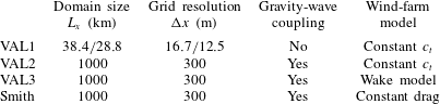
The validation of the three-layer model is organised in three steps with increasing complexity as indicated in table 2. The simulation set-up and validation results of the three validation steps are discussed in the following subsections.
Numerical set-up and model description of the three validation steps and the simulation using the model developed by Smith (Reference Smith2010). Note that the periodic boundary conditions are circumvented in the first validation step (VAL1), and that Smith’s model considers hydrostatic gravity waves and excludes the dependence of the wind-farm drag on the inflow velocity.

3.1 Boundary-layer flow
The first validation step (VAL1) concentrates on the flow in the wind-farm and upper layer, and the pressure disturbance induced by atmospheric gravity waves is replaced by the actual pressure observed in the LES simulations. In this step, we match the numerical set-up of the LES as closely as possible by using the same domain length (38.4 and 28.8 km for the cases of Allaerts & Meyers (Reference Allaerts and Meyers2017) and Allaerts & Meyers (Reference Allaerts and Meyers2018), respectively) and a grid size comparable to the LES resolution, as indicated in table 2. Moreover, as in the LES studies, the periodic boundary conditions are circumvented with a fringe region (see Allaerts & Meyers Reference Allaerts and Meyers2017, Reference Allaerts and Meyers2018, for details of the fringe region set-up).
The background atmospheric state of the three-layer model is prescribed using the procedure explained in § 2.4. For ‘infinitely’ wide wind farms, streamwise turbulent transport is negligible compared to mean-flow transport (Allaerts & Meyers Reference Allaerts and Meyers2017, Reference Allaerts and Meyers2018), so we set the turbulent viscosity coefficients
 $\unicode[STIX]{x1D708}_{t,1}=\unicode[STIX]{x1D708}_{t,2}=0$
. The geostrophic wind velocity
 $\boldsymbol{U}_{g}$
, the Coriolis parameter
 $f_{c}$
, the inversion strength
 $\unicode[STIX]{x0394}\unicode[STIX]{x1D703}$
and the Brunt–Väisälä frequency
 $N$
are chosen to match the LES set-up parameters.
For now, we avoid the complexity of wake models and their coupling with the three-layer model, and instead adopt a very simple wind-farm model with a constant drag coefficient inside the wind-farm region (similar to the simple model developed by Allaerts & Meyers Reference Allaerts and Meyers2018). The wind-farm drag force is thus represented as
 $$\begin{eqnarray}\boldsymbol{f}(x,y)=-c_{t}\unicode[STIX]{x1D6F1}(x,y)\Vert \langle \overline{\boldsymbol{u}}\rangle _{1}\Vert \langle \overline{\boldsymbol{u}}\rangle _{1},\end{eqnarray}$$
with
 $\unicode[STIX]{x1D6F1}(x,y)$
equal to one inside the wind farm and zero everywhere else. Linearising this simple model yields
 $$\begin{eqnarray}\displaystyle & \boldsymbol{f}^{(0)}=-c_{t}\unicode[STIX]{x1D6F1}(x,y)\Vert \boldsymbol{U}_{1}\Vert \boldsymbol{U}_{1}, & \displaystyle\end{eqnarray}$$
 $$\begin{eqnarray}\displaystyle & \displaystyle \boldsymbol{f}^{(1)}=-\frac{c_{t}\unicode[STIX]{x1D6F1}(x,y)}{\Vert \boldsymbol{U}_{1}\Vert }(\boldsymbol{U}_{1}\boldsymbol{U}_{1}+\unicode[STIX]{x1D644}\Vert \boldsymbol{U}_{1}\Vert ^{2})\boldsymbol{\cdot }\boldsymbol{u}_{1}. & \displaystyle\end{eqnarray}$$
The wind-farm drag coefficient
 $c_{t}$
is estimated from the LES results as (Allaerts & Meyers Reference Allaerts and Meyers2018)
 $$\begin{eqnarray}c_{t}=\frac{1}{2}\frac{\unicode[STIX]{x03C0}C_{t}}{4s_{x}s_{y}}\unicode[STIX]{x1D702}_{w}\unicode[STIX]{x1D6FE},\end{eqnarray}$$
with
 $C_{t}$
the turbine thrust coefficient,
 $s_{x}$
and
 $s_{y}$
the streamwise and spanwise turbine spacing relative to the rotor diameter,
 $\unicode[STIX]{x1D702}_{w}$
the wake efficiency and
 $\unicode[STIX]{x1D6FE}=u_{r}^{2}/\Vert \boldsymbol{U}_{1}\Vert ^{2}$
a velocity shape factor with
 $u_{r}$
the rotor-averaged wind speed obtained from LES data.
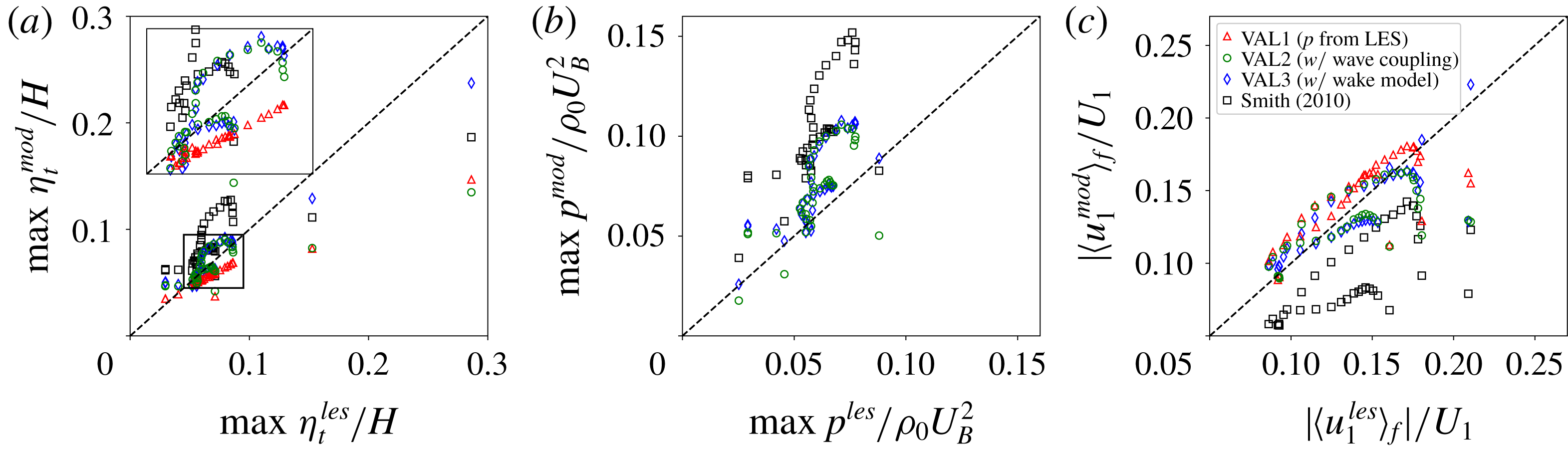
Model prediction versus LES result for 38 data sets (see table 1), showing (a) maximum displacement of the inversion layer relative to the undisturbed inversion height, (b) maximum pressure disturbance and (c) relative velocity reduction averaged over the farm area (denoted by
 $\langle \cdot \rangle _{f}$
). Results for various realisations of the three-layer model are shown, and predictions obtained with the model of Smith (Reference Smith2010) are included for comparison.

Figure 3 gives a global overview of the model performance by comparing model predictions and LES results of three metrics: the maximum displacement of the inversion layer relative to the undisturbed inversion height, the maximum pressure disturbance normalised by the square of the boundary-layer velocity scale
 $U_{B}$
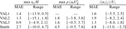
(only for validation step 2 and 3) and the relative velocity reduction with respect to the unperturbed velocity in the wind-farm layer averaged over the farm area. Further, the mean absolute error (MAE) and the error range of the difference between the model and LES predictions for these three metrics are reported in table 3. Results are shown for VAL1, VAL2 and VAL3. For now, we focus on VAL1, other cases are discussed below.
Mean absolute error (MAE) and error range of the difference between model and LES predictions for 38 data sets (see table 1) in terms of maximum displacement of the inversion layer relative to the undisturbed inversion height, maximum pressure disturbance and relative velocity reduction averaged over the farm area (denoted by
 $\langle \cdot \rangle _{f}$
). The results are expressed in percentage points (pp), and positive and negative values in the error range indicate over- and underestimation by the model, respectively.

As can be seen in figure 3 and table 3, the results of the first validation step show very good agreement with the LES data in terms of inversion-layer displacement (MAE of 1.4 percentage points (pp)) and relative velocity reduction (MAE of 1.6 pp). The difference between the model and the LES increases with increasing perturbation values (see e.g. figure 3 a) and is attributed to nonlinear effects.
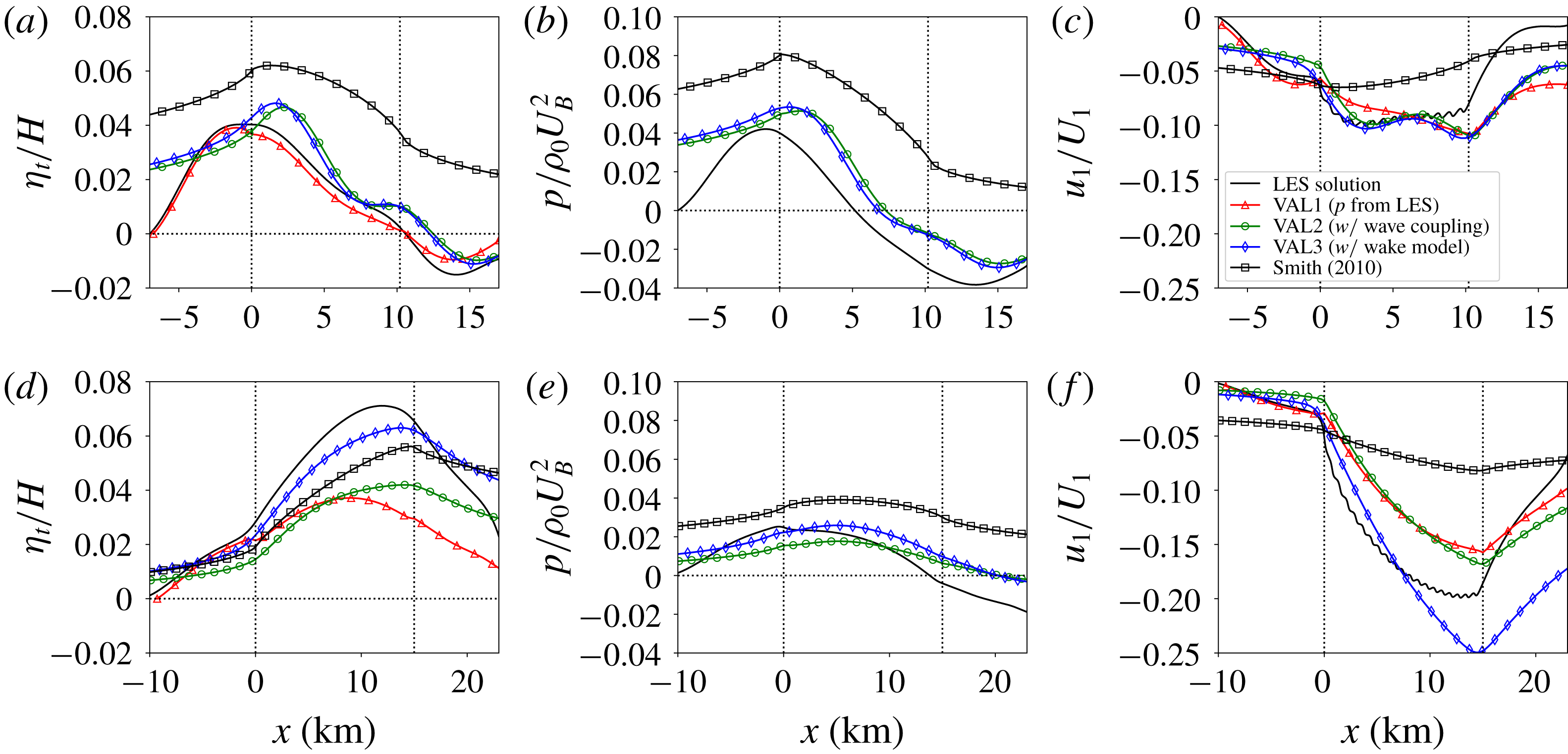
In order to assess the performance of the three-layer model in more detail, figure 4 compares the LES profiles of relative inversion-layer displacement, pressure disturbance and relative velocity reduction with the predictions of the three-layer model for two specific flow cases: case Q00 of Allaerts & Meyers (Reference Allaerts and Meyers2018) and case S1 of Allaerts & Meyers (Reference Allaerts and Meyers2017). Both cases represent neutral boundary-layer flow with a capping inversion at a height of 1 km and a geostrophic wind speed of
 $12~\text{m}~\text{s}^{-1}$
, but differ in terms of surface roughness and inversion strength. We selected these cases because they identify two distinct flow realisations. In case Q00, figure 4(a) shows that the inversion-layer displacement reaches its maximum at the beginning of the farm and falls off in the wind-farm region. On the other hand, for case S1, figure 4(d) indicates that the displacement increases above the wind farm and attains its maximum value near the end of the farm. As we will see later in § 4, the different flow behaviour between these cases is related to the fact that the flow conditions in case Q00 and S1 are subcritical (
 $\mathit{Fr}=0.84$
) and supercritical (
 $\mathit{Fr}=1.94$
), respectively.
Streamwise profiles of (a,d) inversion-layer displacement relative to the undisturbed inversion height, (b,e) pressure disturbance and (c,f) relative velocity reduction for (a–c) case Q00 of Allaerts & Meyers (Reference Allaerts and Meyers2018) and (d–f) case S1 of Allaerts & Meyers (Reference Allaerts and Meyers2017). LES profiles are compared with results from various realisations of the three-layer model and with the model of Smith (Reference Smith2010). The vertical dotted lines mark the start and end of the wind-farm region.

Comparing LES and three-layer model profiles for case Q00 in figure 4(a–c), we observe that the prediction of the first validation step (VAL1) shows excellent agreement with the LES result in terms of inversion-layer displacement. Moreover, the velocity reduction is well reproduced upstream of the farm, while inside the farm the velocity deficit is only slightly underpredicted. Case S1 depicted in figure 4(d–f), on the other hand, appears to be more challenging. The shape of the perturbation is predicted relatively well, but the amplitude is considerably lower than that observed in LES. This difference may be related to the use of a simple wind-farm model with constant drag coefficient (cf. e.g. the model predictions of VAL3 which uses a more complex wake model, further discussed below).
3.2 Gravity-wave-induced pressure
In the second validation step (VAL2), we include the pressure feedback of the inversion layer and the free atmosphere but adhere to the simple wind-farm model discussed above. Since the expression for the internal-gravity-wave pressure (cf. (2.24) and (2.25)) results from analytically solving perturbation equations in the free atmosphere, it is no longer possible to simply insert a fringe region in the three-layer model. Instead, we use a numerical domain of 1000 km at a grid resolution of 300 m to allow the perturbations to die out before being recycled by the periodic boundary conditions (see table 2). The background atmospheric state and wind-farm drag coefficient are determined as in § 3.1.
We also compare the performance of the three-layer model with the model developed by Smith (Reference Smith2010), which is comprised of only two layers, i.e. the boundary layer and the free atmosphere (see appendix C for a brief description). The atmospheric state of this model is determined using the procedure outlined in § 2.4, but now vertical averages are taken over the entire boundary layer. The same numerical set-up is used, i.e. a domain of 1000 km at a grid resolution of 300 m (see table 2). Smith’s model only allows for a zero-order wind-farm model, so we only use (3.2) and specify the wind-farm drag coefficient with (3.4).
The results of the second validation step are included in figure 3 and table 3 and show that the agreement with LES remains very good upon including the feedback of gravity waves (MAE of VAL1 and VAL2 are similar and the error range increases slightly). Moreover, the predictions of the three-layer model are considerably better than those of Smith’s model, which systematically overpredicts the inversion-layer displacement and pressure disturbance and performs poorly in terms of relative velocity reduction (MAE of 4.8 pp with Smith’s model compared to 1.9 pp with VAL2).
Considering the streamwise perturbation profiles for case Q00 in figure 4(a–c), validation step 2 performs relatively well in terms of perturbation shape and amplitude for both displacement and pressure. As mentioned before, we find too large values of displacement and pressure perturbation when using Smith’s model. In terms of velocity reduction, the predictions of validation step 2 are comparable to those obtained in step 1, with a general underestimation upstream of the farm. Smith’s model, by contrast, strongly underpredicts the velocity reduction inside the farm. Further, we note that a spatial lag appears to exist between the model and LES predictions (compare, e.g., the predicted location of the maximum inversion-layer displacement). However, it is unclear whether this is a modelling error due to the simplification of the three-layer model or an artefact of the LES caused by the limited numerical domain and the boundary conditions. For case S1 in figure 4(d–f), on the other hand, the perturbation profiles obtained with validation step 1 and 2 are very similar, i.e. the main trends are captured but the amplitude is underestimated. Smith’s model appears to predict the inversion-layer displacement relatively well for this case, but the estimates of the pressure and velocity reduction are in bad agreement with the LES.
Finally, both in case Q00 and case S1, we observe that the asymptotic behaviour far upstream of the wind farm obtained with either the three-layer model or Smith’s model is considerably different from the asymptotic behaviour in the LES results. The difference is likely due to the limited LES domain and the use of a fringe region, which sets the perturbations artificially to zero at the boundaries. Evidence for this argument is found in the good agreement of the upstream flow behaviour between the LES solution and the results from VAL1 (see figure 4), where the latter validation step used the exact same numerical domain size and artificial fringe region as the LES. By contrast, the results of both VAL2 and Smith’s model are obtained on a much larger domain without a fringe region to allow the perturbations to die out at their own natural pace. For this reason, we believe that the proper asymptotic behaviour far upstream is shown by the boundary-layer model while the LES tends to compress the upstream slow down in a smaller region due to the imposed boundary conditions (a similar observation was made by Allaerts & Meyers (Reference Allaerts and Meyers2018) based on a simple two-layer model).
3.3 Coupling with wake model
In the third step of the validation process (VAL3), we evaluate the coupling of the three-layer model with the Gaussian-wake model. This means that the wind-farm drag force is now calculated only based on turbine locations, diameters and thrust coefficients, while before the wake efficiency needed to be specified a priori with LES data (see (3.1)). The numerical set-up is the same as in validation step 2 (see table 2).
Figure 3 shows that the model predictions using the simple wind-farm model (VAL2) and the Gaussian-wake model (VAL3) agree remarkably well, and in some cases the wake model even outperforms the simple model. This is also reflected in reduced mean absolute errors and reduced error ranges in table 3. The agreement between validation step 2 and 3 is very promising as the wake model does not depend on LES information to specify the wake efficiency. Figure 4 further shows that for case Q00, the results of validation step 2 and 3 are almost identical. The difference between the two validation steps is larger for case S1, for which the results using the Gaussian-wake model better predict the amplitude of the flow perturbation.
We conclude that the three-layer model coupled with the Gaussian wake model performs reasonably well and can be used to obtain a conservative estimate of gravity-wave-induced effects. However, it is important to bear in mind that the model has only been validated based on two-dimensional LES profiles. A full three-dimensional validation with large-eddy simulations of finite-size wind farms is a topic for further research.
4 Flow physics
In this section, we aim to comprehend the flow physics induced by the three-layer model. To this end, we derive and analyse the equation for the total displacement in § 4.1 and investigate the simulated flow patterns for two relevant cases in § 4.2.
4.1 Total displacement equation
An equation for the total displacement
 $\unicode[STIX]{x1D702}_{t}$
is obtained by summing the divergence of the momentum equations (2.17) and (2.18) scaled with
 $H_{1}/U_{1}^{2}$
and
 $H_{2}/U_{2}^{2}$
, respectively, and substituting the continuity equations (2.19) and (2.20) and the expressions for the gravity-wave pressure (2.23) and (2.24) in the result. In a coordinate frame aligned with the flow in the wind-farm layer and assuming that the directional shear in the boundary layer is small (i.e. taking
 $V_{2}=V_{1}=0$
), we find
 $$\begin{eqnarray}(-1+\mathit{Fr}^{-2}+{P_{N}}^{-1}{\mathcal{G}})\frac{\unicode[STIX]{x2202}^{2}\unicode[STIX]{x1D702}_{t}}{\unicode[STIX]{x2202}x^{2}}+(\mathit{Fr}^{-2}+{P_{N}}^{-1}{\mathcal{G}})\frac{\unicode[STIX]{x2202}^{2}\unicode[STIX]{x1D702}_{t}}{\unicode[STIX]{x2202}y^{2}}=\frac{H_{1}}{U_{1}^{2}}\unicode[STIX]{x1D735}\boldsymbol{\cdot }RHS_{1}+\frac{H_{2}}{U_{2}^{2}}\unicode[STIX]{x1D735}\boldsymbol{\cdot }RHS_{2},\end{eqnarray}$$
with
 ${\mathcal{G}}$
a linear operator (defined further below). The terms
 $RHS_{1}$
and
 $RHS_{2}$
denote the right-hand sides of (2.17) and (2.18), respectively, and depend on the variables
 $\boldsymbol{u}_{1}$
and
 $\boldsymbol{u}_{2}$
, and therefore indirectly on
 $\unicode[STIX]{x1D702}_{t}$
, but not on the derivatives of these variables (except for the turbulent diffusion term, which is generally small). Consequently, the right-hand side of (4.1) depends indirectly on
 $\unicode[STIX]{x2202}\unicode[STIX]{x1D702}_{t}/\unicode[STIX]{x2202}x$
and
 $\unicode[STIX]{x2202}\unicode[STIX]{x1D702}_{t}/\unicode[STIX]{x2202}y$
but not on higher-order derivatives of the displacement. On the left-hand side of (4.1), the minus one originates from the convective terms in the momentum equations. Further, in agreement with the results of Smith (Reference Smith2010), we find that the effect of the pressure induced by interfacial and internal waves is governed by the non-dimensional numbers
 $\mathit{Fr}=U_{B}/\sqrt{g^{\prime }H}$
(a Froude number) and
 $P_{N}=U_{B}^{2}/NH\Vert \boldsymbol{U}_{g}\Vert$
, respectively. The velocity scale
 $U_{B}$
is thereby defined as
 $$\begin{eqnarray}U_{B}=\left(\frac{H_{1}}{H}\frac{1}{U_{1}^{2}}+\frac{H_{2}}{H}\frac{1}{U_{2}^{2}}\right)^{-1/2},\end{eqnarray}$$
and reflects the fact that the flow convergence or divergence and hence the change in depth of the wind-farm and upper layer for a given perturbation (a pressure gradient, frictional drag or an external force) is proportional to the height and inversely proportional to the square of the velocity of the respective layer. For example, a high upper-layer velocity
 $U_{2}$
implies that the change in depth
 $\unicode[STIX]{x1D702}_{2}$
of that layer is very small and that the boundary-layer response mainly comes from the wind-farm layer, so
 $U_{B}^{2}/H\simeq U_{1}^{2}/H_{1}$
. Note that the same expression for
 $U_{B}$
is found when deriving the characteristics of the original set of equations (2.17)–(2.20) (see appendix D).
Consider first the flow behaviour induced by (4.1) in the absence of internal gravity waves (i.e. for
 $P_{N}\rightarrow \infty$
). The governing equation is then a classic partial differential equation (PDE) of second order leading to flow physics that are very similar to shallow-water flow. The behaviour of such a system is governed by the Froude number and is categorised as being subcritical (
 $\mathit{Fr}<1$
, (4.1) is an elliptic PDE), critical (
 $\mathit{Fr}=1$
, parabolic PDE) or supercritical (
 $\mathit{Fr}>1$
, hyperbolic PDE). The Froude number can also be interpreted as the ratio of the boundary-layer velocity scale
 $U_{B}$
to the wave speed of the interfacial waves. Hence, interfacial waves can propagate against the flow and affect upstream wind conditions in subcritical conditions, while in supercritical conditions interfacial waves only affect the flow downstream of the perturbation.
We now investigate the effect of the internal gravity waves. The amplitude of these waves is governed by the non-dimensional number
 $P_{N}$
and increases for decreasing values of
 $P_{N}$
. The spatial distribution of their impact is determined by the linear operator
 ${\mathcal{G}}$
, which is defined as
 $$\begin{eqnarray}{\mathcal{G}}(\unicode[STIX]{x1D702}_{t})=\frac{\unicode[STIX]{x1D6F7}}{N\Vert \boldsymbol{U}_{g}\Vert }\ast \unicode[STIX]{x1D702}_{t},\end{eqnarray}$$
where
 $\ast$
denotes the convolution operation and
 $\unicode[STIX]{x1D6F7}={\mathcal{F}}^{-1}(\hat{\unicode[STIX]{x1D6F7}})$
is the inverse Fourier transform of the complex stratification coefficient
 $\hat{\unicode[STIX]{x1D6F7}}$
defined in (2.25). The rationale for the factor
 $N\Vert \boldsymbol{U}_{g}\Vert$
in the linear operator is that the surface pressure induced by hydrostatic gravity waves excited by a symmetric perturbation scales linearly with this factor (Smith Reference Smith1980). In the general non-hydrostatic case, we find that the scaling still applies provided that the excited wave field is close to hydrostatic. This condition is met when the horizontal wavenumber
 $\unicode[STIX]{x1D705}_{H}$
of the strongest or most excited wave (which is inversely proportional to the characteristic horizontal length scale of the displacement
 $a$
) is small compared to the Scorer parameter
 $L_{s}=N/\Vert \boldsymbol{U}_{g}\Vert$
(Nappo Reference Nappo2002), i.e. when
 $aN/\Vert \boldsymbol{U}_{g}\Vert \gg 1$
. This is generally true for wind-farm flow cases where typical values are
 $a=10~\text{km}$
,
 $N=0.01~\text{s}^{-1}$
and
 $\Vert \boldsymbol{U}_{g}\Vert =10~\text{m}~\text{s}^{-1}$
so that
 $aN/\Vert \boldsymbol{U}_{g}\Vert =10$
.
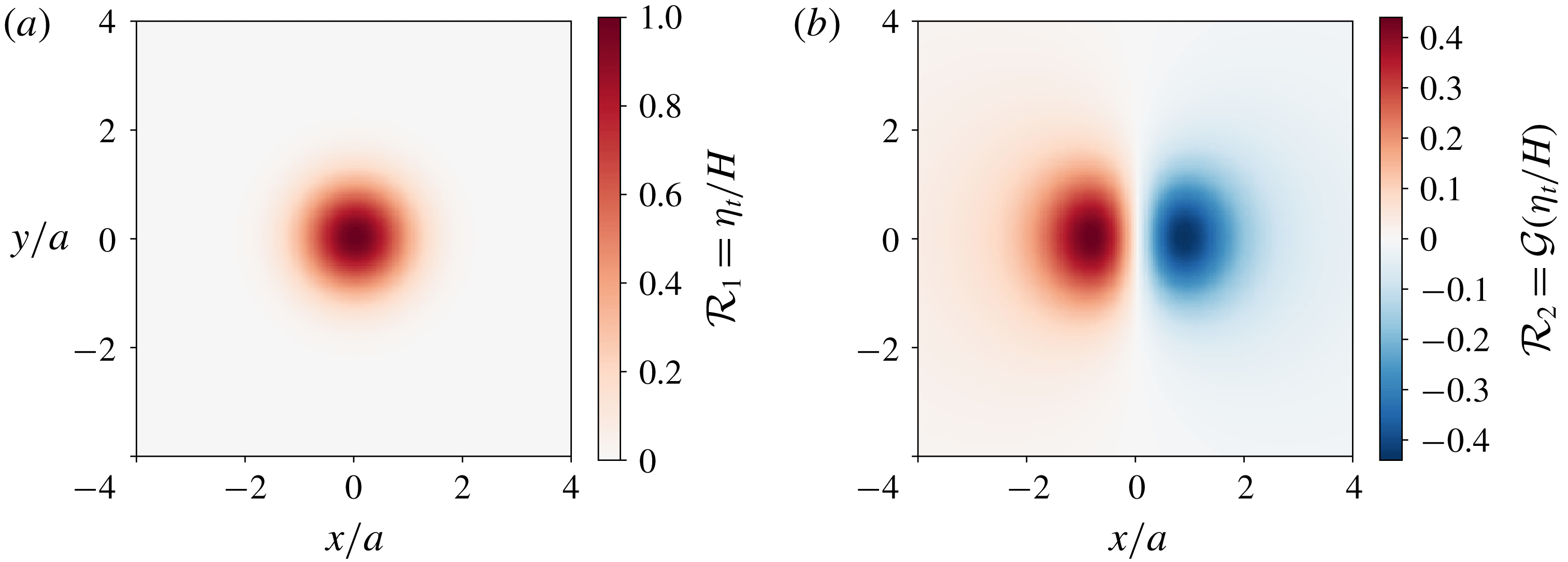
Geometric footprint of the pressure perturbation over a Gaussian displacement
 $\unicode[STIX]{x1D702}_{t}/H=\exp [-(x/a)^{2}-(y/a)^{2}]$
induced by (a) gravity waves on the interface between the upper layer and the free atmosphere (i.e.
 ${\mathcal{R}}_{1}$
) and (b) gravity waves in the free atmosphere (i.e.
 ${\mathcal{R}}_{2}$
). The geometric footprints are defined in (4.4). The geostrophic wind is directed in the positive
 $x$
-direction and
 $aN/\Vert \boldsymbol{U}_{g}\Vert =10$
.

In order to gain insight in the spatial distribution implied by (4.3), figure 5 illustrates the geometric footprint of the pressure induced by interfacial waves and internal gravity waves in response to a Gaussian displacement
 $\unicode[STIX]{x1D702}_{t}/H=\exp [-(x/a)^{2}-(y/a)^{2}]$
with
 $aN/\Vert \boldsymbol{U}_{g}\Vert =10$
and the geostrophic wind directed in the positive
 $x$
-direction. The geometric footprint
 ${\mathcal{R}}$
of the wave response is thereby defined as the pressure induced by the waves scaled with
 $\unicode[STIX]{x1D70C}_{0}U_{B}^{2}$
and the governing non-dimensional number, which is either
 $\mathit{Fr}^{-2}$
or
 ${P_{N}}^{-1}$
(see (4.1)):
 $$\begin{eqnarray}{\mathcal{R}}_{1}\equiv \frac{p_{1}}{\unicode[STIX]{x1D70C}_{0}U_{B}^{2}\mathit{Fr}^{-2}}=\frac{\unicode[STIX]{x1D702}_{t}}{H}\quad \text{and}\quad {\mathcal{R}}_{2}\equiv \frac{p_{2}}{\unicode[STIX]{x1D70C}_{0}U_{B}^{2}{P_{N}}^{-1}}={\mathcal{G}}\left(\frac{\unicode[STIX]{x1D702}_{t}}{H}\right).\end{eqnarray}$$
Since the pressure induced by interfacial waves scales linearly with the displacement (see (2.23)), the footprint is identical to the displacement and thus has the same symmetry. In contrast, the pressure distribution induced by the internal gravity waves is highly anisotropic, with large pressure gradients in the direction of the geostrophic wind and considerably lower lateral pressure gradients on the sides of the displacement. Moreover, the horizontal extent of the internal gravity waves is larger than that of the interfacial waves both in upstream and downstream direction (with respect to the geostrophic wind direction).
4.2 Gravity-wave-induced flow patterns
We investigate the impact of gravity waves on upstream and downstream wind conditions in more detail by analysing the gravity-wave-induced flow patterns for a relevant sub- and supercritical flow case. The particular choice of atmospheric state and wind-farm configuration is motivated later in § 5 (details of this reference set-up are summarised in table 4). For now, it suffices to know that
 $P_{N}=2.2$
and that
 $\mathit{Fr}=0.9$
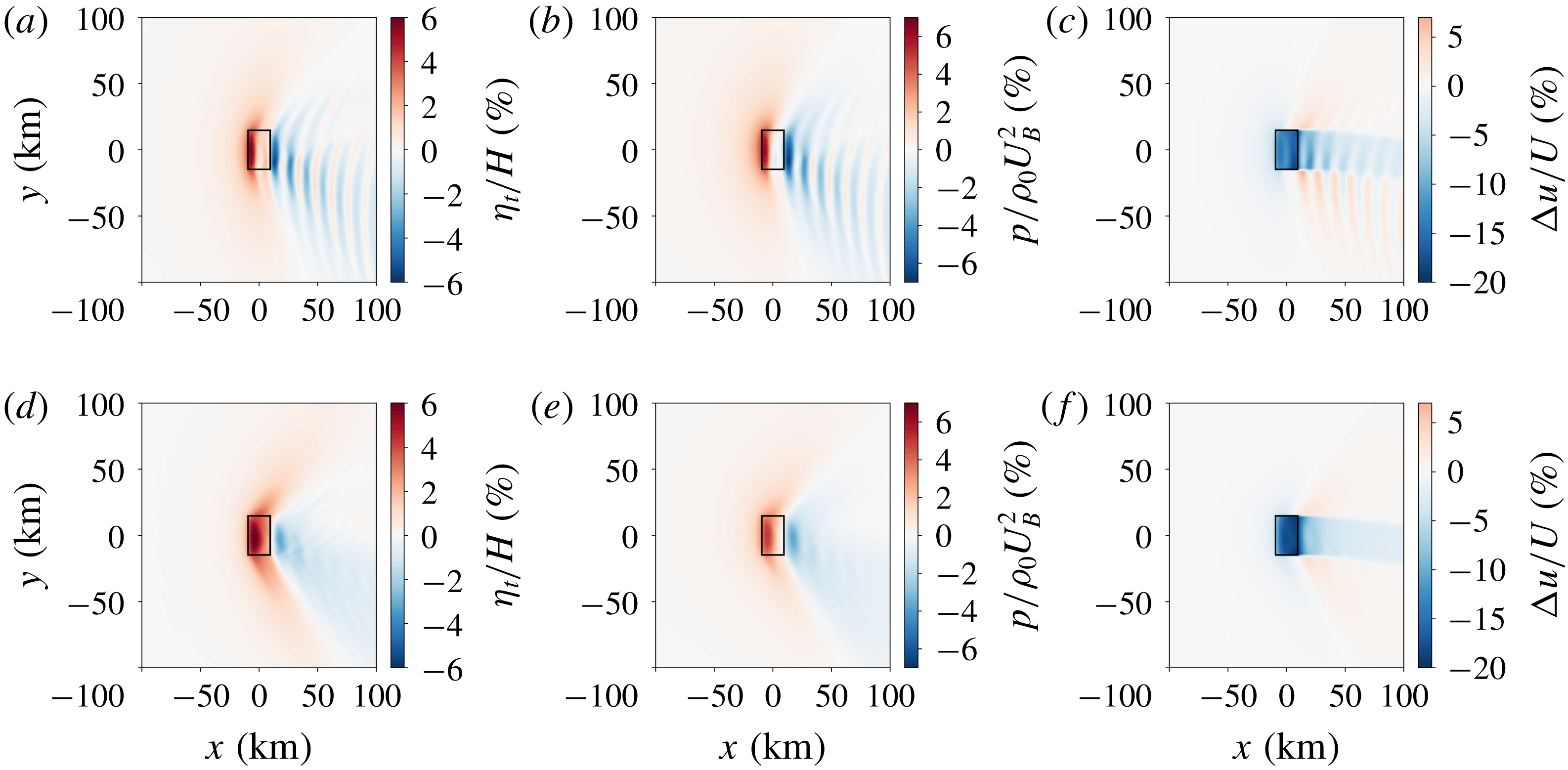
and 1.1 in the sub- and supercritical case, respectively. The simulation results for these two cases are visualised in figure 6, showing a planform view of the inversion-layer displacement, the pressure perturbation and the relative velocity reduction in the wind-farm layer.
Planform view of (a,d) inversion-layer displacement relative to the undisturbed inversion height, (b,e) pressure disturbance and (c,f) relative velocity reduction in the wind-farm layer, for a subcritical (a,b,c,
 $\mathit{Fr}=0.9$
) and supercritical flow case (d,e,f,
 $\mathit{Fr}=1.1$
). The black rectangle indicates the wind-farm region.

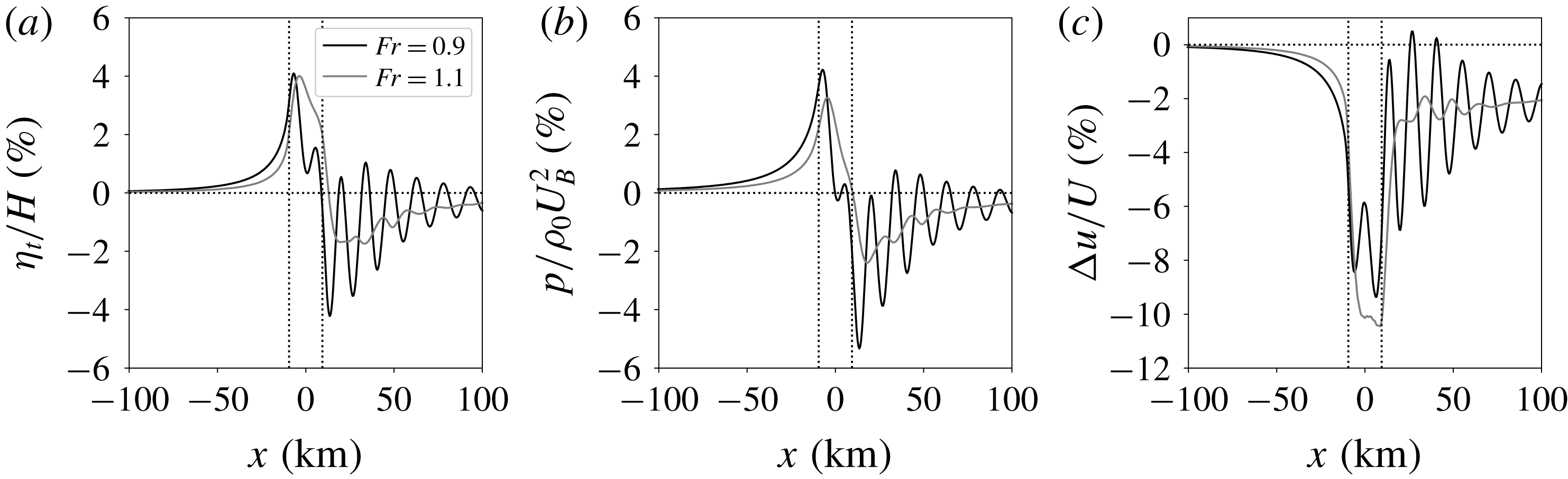
Upstream of the wind farm, the contrast between the sub- and supercritical flow fields is very subtle. The difference between both cases can be seen more clearly in figure 7, showing streamwise profiles through the centre of the farm. The maximum inversion displacement is shown to be almost equal in both cases, but the location of the maximum perturbation lies closer to the farm entrance in the subcritical case, which is in agreement with the earlier observation made in § 3 comparing figures 4(a) and 4(d). As a result, the influence of the wind farm extends further upstream in the subcritical case, and this finding also holds for the pressure and velocity perturbations. The difference between the sub- and supercritical flow case is caused by the fact that in supercritical conditions, the upstream influence comes solely from internal gravity waves, while in subcritical conditions, interfacial waves can travel upstream as well (Smith Reference Smith2010). Interestingly, we find that the inversion displacement (and also the pressure and velocity perturbation) in both the sub- and supercritical flow cases decays upstream with an e-folding length scale of the order of 12 km.
Streamwise profiles of (a) inversion-layer displacement relative to the undisturbed inversion height, (b) pressure disturbance and (c) relative velocity reduction in the wind-farm layer, for a subcritical (black line,
 $\mathit{Fr}=0.9$
) and supercritical flow case (grey line,
 $\mathit{Fr}=1.1$
). The wind-farm region is marked by vertical dashed lines, and the profiles have been obtained in the centre of the farm.

In the downstream direction, there is a clear distinction between the sub- and supercritical flow fields shown in figure 6. In the supercritical case, we observe several distinct V-shapes formed by pairs of characteristic lines of the governing PDE system (see appendix D for a discussion on the characteristics of the three-layer model). A first V-shape with positive displacement and pressure perturbation starts at the front of the farm. Behind the farm, the absence of wind-farm drag gives rise to a second V-shape, this time with negative displacement and pressure perturbation values. The transition from positive to negative pressure perturbations leads to a favourable pressure gradient, which accelerates the flow outside the wind-farm wake as seen in figure 6(f). For our model, the pair of characteristic lines leading to the V-shaped patterns is expressed by ((D 6) with
 $\unicode[STIX]{x1D713}=0$
)
 $$\begin{eqnarray}\frac{\text{d}y}{\text{d}x}=\pm \frac{1}{\sqrt{\mathit{Fr }^{2}-1}}.\end{eqnarray}$$
According to (4.5), the characteristic lines should form an angle of
 $\pm 63^{\circ }$
with the
 $x$
-axis for
 $\mathit{Fr}=1.1$
, and this prediction corresponds well with the observed flow patterns in figure 6(d–f).
In the subcritical case, the characteristics given by (4.5) become imaginary, and hence no V-shaped patterns occur downstream of the wind farm. Instead, we observe that the wind farm excites resonant lee waves. These are evanescent gravity waves (with vertical wavenumber
 $m$
imaginary) for which the coefficient of the first term in (4.1) becomes zero:
 $$\begin{eqnarray}-1+\mathit{Fr}^{-2}+\frac{H}{U_{B}^{2}}\frac{\text{i}(N^{2}-\unicode[STIX]{x1D6FA}^{2})}{m}=0.\end{eqnarray}$$
Physically, this means that the flow advection is exactly balanced by the sum of pressure contributions from interfacial and internal gravity waves. Upon substituting the expression for the vertical wavenumber
 $m$
(see (2.26)), we find that resonant lee waves only exist for
 $\mathit{Fr}<1$
, and the horizontal wavenumber is in that case given by
 $$\begin{eqnarray}\frac{\unicode[STIX]{x1D73F}_{H}\boldsymbol{\cdot }\boldsymbol{U}_{g}}{N}=\sqrt{1+P_{N}^{2}(\mathit{Fr }^{-2}-1)^{2}(\cos \unicode[STIX]{x1D6FD})^{-2}},\end{eqnarray}$$
with
 $\unicode[STIX]{x1D6FD}$
the angle between the horizontal wave vector and the geostrophic wind. For example, in the subcritical case, equation (4.7) predicts a wavelength of 14.1 km along the
 $x$
-direction. This prediction appears to agree well with the flow patterns in figure 6(a–c) and the streamwise profiles shown in figure 7. Moreover, we find a local maximum at a wavelength of 14.7 km in the one-dimensional wavenumber spectrum of the streamwise inversion-layer displacement profile (not shown), confirming the visual agreement.
Finally, figure 6(c,f) shows that the wind-farm wake is deflected towards the right in both cases, which agrees with the findings of previous wind-farm studies (van der Laan & Sørensen Reference van der Laan and Sørensen2017; Allaerts & Meyers Reference Allaerts and Meyers2018). The wake deflection is caused by momentum exchange with the flow in the upper layer, which has a relative wind direction towards the right.
5 Sensitivity analysis
We now investigate how the atmospheric state and the wind-farm configuration influence the excitation of gravity waves, and we identify the regimes in which gravity-wave-induced power loss is significant. We thereby start from a reference set-up and systematically vary the relevant non-dimensional groups. The reference set-up is described and motivated in § 5.1, and the sensitivity with respect to atmospheric state and wind-farm configuration is discussed in §§ 5.2 and 5.3, respectively.
5.1 Reference wind-farm configuration and atmospheric state
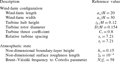
We consider a generic rectangular wind farm with length
 $a_{x}=20~\text{km}$
and width
 $a_{y}=30~\text{km}$
. These dimensions are of the same order of magnitude as those used in previous wind-farm gravity-wave studies (Smith Reference Smith2010; Fitch et al.
Reference Fitch, Olson, Lundquist, Dudhia, Gupta, Michalakes and Barstad2012; Wu & Porté-Agel Reference Wu and Porté-Agel2017) and correspond roughly to the area covered by the Belgian–Dutch wind-farm cluster, comprised of the Belgian offshore wind-farm zone and the adjacent Borssele wind-farm zone located in the Exclusive Economic Zone of the Netherlands. We place 486 8-MW wind turbines in the farm so that the total capacity is 3888 MW, which is approximately the same as the planned installed capacity of the Belgian–Dutch wind-farm cluster. The wind turbines are arranged in 18 rows and 27 columns in a staggered pattern with respect to the
 $x$
-direction. The turbine dimensions are based on a Siemens SWT-8.0-154 wind turbine with turbine hub height
 $z_{h}=120~\text{m}$
and rotor diameter
 $D=154~\text{m}$
. Further, we assume that all turbines operate at a constant thrust coefficient
 $C_{t}=0.8$
. The relative turbine spacing is
 $s_{x}=s_{y}\simeq 7.21$
. We non-dimensionalise the wind-farm set-up with
 $H=1000~\text{m}$
, which is the typical order of magnitude of the atmospheric boundary-layer height (Stull Reference Stull1988; Hess Reference Hess2004). The reference wind-farm configuration is summarised in table 4.
Reference wind-farm configuration and atmospheric state used throughout the current study. The reference sub- and supercritical cases used in §§ 4.2 and 5.3 are obtained by setting the inversion parameter
 $g^{\prime }H/Au_{\ast }^{2}$
equal to 1.04 and 0.69, leading to Froude numbers of 0.9 and 1.1, respectively.

The atmospheric conditions of the three-layer model are prescribed with the analytical boundary-layer model derived by Nieuwstadt (Reference Nieuwstadt1983). More specifically, we employ Nieuwstadt’s solution of the Ekman-layer equations with a cubic turbulent viscosity profile
 $\unicode[STIX]{x1D708}_{T}=\unicode[STIX]{x1D705}u_{\ast }z(1-z/H)^{2}$
and set the von Kármán constant
 $\unicode[STIX]{x1D705}=0.41$
. In combination with the corresponding resistance laws (also derived by Nieuwstadt), this model provides values for the geostrophic wind direction and the geostrophic drag as well as vertical profiles of velocity and turbulent stress (see Allaerts & Meyers Reference Allaerts and Meyers2015, for practical details). From these profiles, the depth-averaged velocities and the friction and turbulent viscosity coefficients are determined using the procedure elaborated in § 2.4.
The input parameters to Nieuwstadt’s model are the non-dimensional surface roughness length
 $\bar{z}_{0}=z_{0}/H$
and the non-dimensional boundary-layer height
 $h_{\ast }=Hf_{c}/u_{\ast }$
. The surface roughness parameter can vary several orders of magnitude depending on underlying terrain type, and here we consider a relatively broad range between
 $10^{-8}$
and
 $10^{-2}$
. On the other hand, typical values for
 $h_{\ast }$
go from 0.1 for shallow boundary layers over sea to 0.35 for deep land-based boundary layers (Hess Reference Hess2004). In order to study a wide range of boundary-layer heights, we vary
 $h_{\ast }$
between 0.06 and 0.5. Note that Nieuwstadt’s model actually depends on
 $h_{\ast }/\unicode[STIX]{x1D705}$
, which can be interpreted either as the ratio of the actual boundary-layer height to the neutral scale height
 $\unicode[STIX]{x1D705}u_{\ast }/f_{c}$
or in terms of thermal stability, i.e. an increase in the turbulent viscosity (through the parameter
 $\unicode[STIX]{x1D705}$
) due to stability effects has the same impact on the shear stress and the convexity of the velocity profile as a decrease in boundary-layer height.
The Brunt–Väisälä frequency
 $N$
and the reduced gravity
 $g^{\prime }$
also need to be specified. The Brunt–Väisälä frequency is determined by the free atmosphere stratification, which typically lies between 1 and
 $10~\text{K}~\text{km}^{-1}$
(Sorbjan Reference Sorbjan1996). Here, we explore a wider range of 0.01–
 $100~\text{K}~\text{km}^{-1}$
, corresponding to
 $N/f_{c}$
between 5.8 and 580 (with
 $f_{c}=10^{-4}~\text{s}^{-1}$
and
 $\unicode[STIX]{x1D703}_{0}=15\,^{\circ }\text{C}$
). For the reduced gravity, we use the empirical result of Csanady (Reference Csanady1974) stating that the inversion parameter
 $g^{\prime }H/Au_{\ast }^{2}\gtrsim 1$
in equilibrium conditions, with the empirical constant
 $A=500$
(Csanady Reference Csanady1974; Tjernström & Smedman Reference Tjernström and Smedman1993). Values lower than unity may correspond to non-equilibrium conditions or cases with large-scale subsidence.
In summary, the atmospheric conditions are governed by the non-dimensional numbers
 $$\begin{eqnarray}h_{\ast },\quad \bar{z}_{0},\quad \frac{N}{f_{c}}\quad \text{and}\quad \frac{g^{\prime }H}{Au_{\ast }^{2}},\end{eqnarray}$$
and we take
 $h_{\ast }=0.15$
,
 $\bar{z}_{0}=10^{-4}$
and
 $N/f_{c}=58$
as the base state (see table 4). Further, we set the inversion parameter
 $g^{\prime }H/Au_{\ast }^{2}$
equal to 1.04 and 0.69 to obtain reference sub- and supercritical cases with Froude numbers of 0.9 and 1.1, respectively. Note that the analysis of gravity-wave-induced flow patterns in § 4.2 was based on these two cases.
The three-layer model is solved on a two-dimensional numerical domain of
 $1000H\times 400H$
with a uniform grid resolution of
 $0.5H$
, corresponding to 1.6 M grid cells per layer. A grid sensitivity study shows that the outcome varies by less than 1 % when the numerical domain size or the grid resolution is modified (see § A.4). The coordinate axis is chosen such that the wind in the wind-farm layer is always directed along the
 $x$
-axis and perpendicular to one of the sides of the rectangular wind farm. Note that wind-farm orientation relative to the wind direction or more general wind-farm shapes is likely to affect gravity-wave excitation. The sensitivity to these parameters is very case-specific, however, and lies outside the current scope.
5.2 Sensitivity to atmospheric state
In order to investigate the sensitivity of wind-farm-induced gravity waves to atmospheric conditions, we start from the base atmospheric state and systematically vary
 $h_{\ast }$
,
 $\bar{z}_{0}$
or
 $N/f_{c}$
against the inversion parameter
 $g^{\prime }H/Au_{\ast }^{2}$
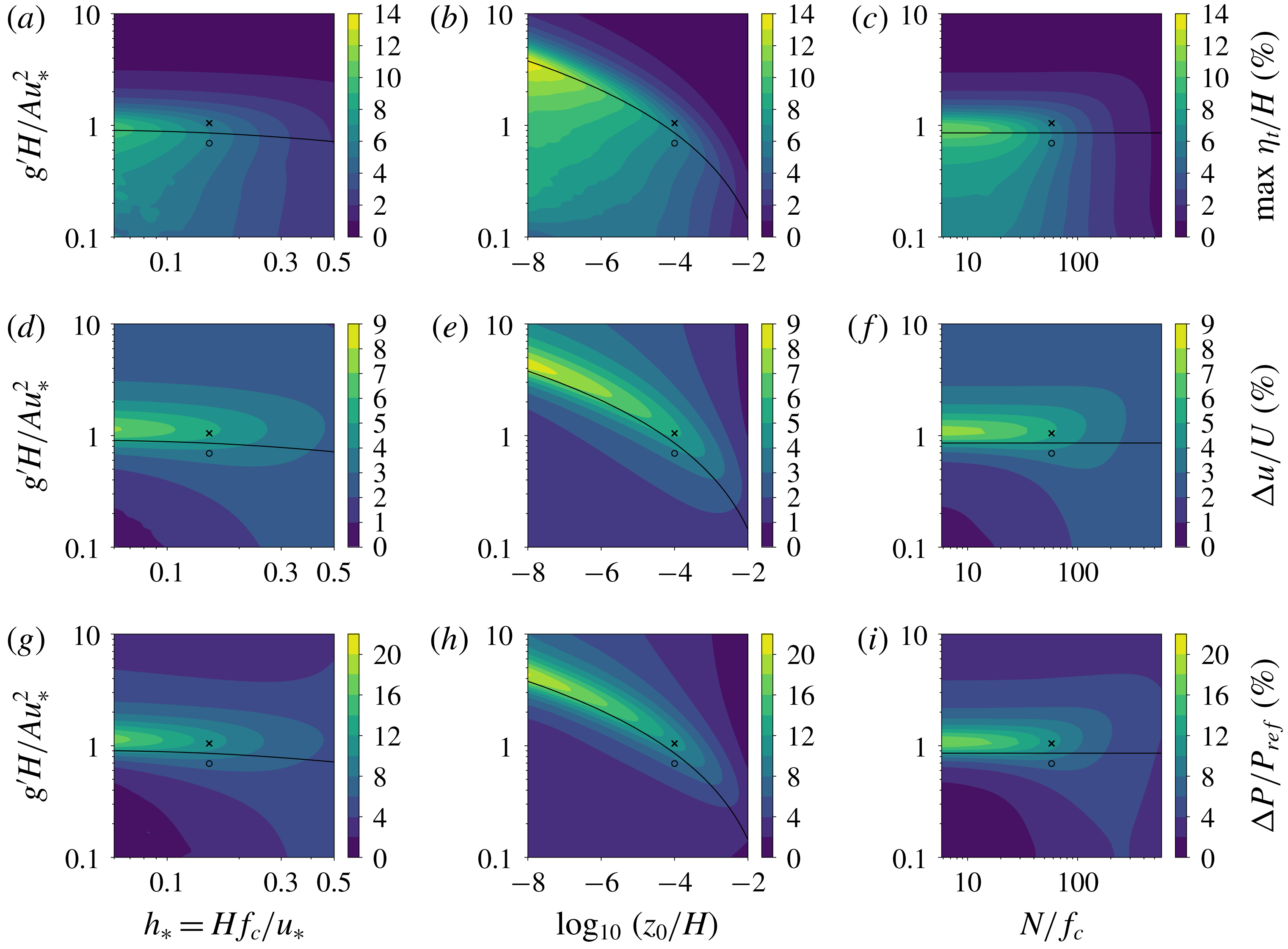
. The results are illustrated in figure 8 in terms of maximum boundary-layer displacement (a–c), upstream velocity reduction (d–f) and power loss due to gravity waves (g–i). The latter is calculated with respect to the power output of the same wind farm in the absence of gravity waves but including wake effects, and it is a direct measure for the importance of gravity-wave feedback effects. Figure 8 also shows the contour line for
 $\mathit{Fr}=1$
(solid black line). Lines of constant Froude number run parallel to this line (not shown), with sub- and supercritical flow conditions above and below the critical flow line, respectively. The reference sub- and supercritical flow cases are marked with an x and an o symbol, respectively.
Sensitivity of wind-farm gravity waves to atmospheric conditions in terms of (a–c) maximum boundary-layer displacement, (d–f) velocity reduction, taken 1 km upstream and averaged over the width of the farm, and (g–i) power loss due to the gravity-wave feedback effect (i.e. compared to the power output without gravity waves). The results are shown as a function of the inversion parameter
 $g^{\prime }H/Au_{\ast }^{2}$
versus (a,d,g) the non-dimensional boundary-layer height
 $h_{\ast }$
(with
 $\bar{z}_{0}=10^{-4}$
and
 $N/f_{c}=58$
), (b,e,h) the logarithm of the non-dimensional surface roughness length
 $\bar{z}_{0}$
(with
 $h_{\ast }=0.15$
and
 $N/f_{c}=58$
) and (c,f,i) the ratio of Brunt–Väisälä frequency to Coriolis parameter
 $N/f_{c}$
(with
 $h_{\ast }=0.15$
and
 $\bar{z}_{0}=10^{-4}$
). The black solid line in each panel corresponds to critical flow conditions (
 $\mathit{Fr}=1$
), and sub- and supercritical flow are found above and below this line, respectively. The symbols represent the reference subcritical (x marker) and supercritical (o marker) flow cases.

Consider first figure 8(a–c) displaying the maximum boundary-layer displacement. This metric can be viewed as a proxy for the wave amplitude and indicates that, for a given value of the inversion parameter
 $g^{\prime }H/Au_{\ast }^{2}$
, the excitation of gravity waves appears to decrease with increasing boundary-layer height, surface roughness and free atmosphere stratification. On the other hand, we find that the highest sensitivity in terms of the inversion parameter for any combination of
 $h_{\ast }$
,
 $\bar{z}_{0}$
and
 $N/f_{c}$
always concurs with the solid black line, meaning that the excitation of gravity waves is maximal when the flow is critical. The inversion parameter leading to critical flow conditions increases with decreasing boundary-layer height and particularly with decreasing surface roughness. For the current wind-farm configuration, the relative displacement is typically 10 % or less, except for very low values of surface roughness or free atmosphere stratification, for which the relative displacement can be as high as 14 % in critical flow conditions.
The trends observed in the sensitivity of the boundary-layer displacement are related to the shallow-water-like flow physics induced by the inversion layer (cf. § 4.1). In the absence of internal gravity waves and frictional effects, the ABL behaves likes an idealised shallow-water system and any external force would induce very large flow perturbations for
 $\mathit{Fr}\rightarrow 1$
. This is the choking effect discussed by Smith (Reference Smith2010) and explains why the highest gravity-wave excitation occurs for critical flow conditions in figure 8(a–c).
The departure from the idealised shallow-water flow conditions is regulated by the parameters
 $h_{\ast }$
,
 $\bar{z}_{0}$
and
 $N/f_{c}$
, which introduce frictional drag and internal gravity waves. Increasing values of
 $h_{\ast }$
and especially
 $\bar{z}_{0}$
enhance the frictional drag, which dissolves the singularity at critical Froude numbers by dissipating perturbation energy. Internal gravity waves also tend to disperse the choking effect of interfacial waves (Allaerts & Meyers Reference Allaerts and Meyers2018). As discussed in § 4.1, the amplitude of these waves increases with decreasing values of
 $P_{N}=U_{B}^{2}/NH\Vert \boldsymbol{U}_{g}\Vert$
. A rise in
 $N/f_{c}$
thus leads the flow physics away from the singularity and results in reduced flow perturbations. Similarly, changing the parameters
 $h_{\ast }$
and
 $\bar{z}_{0}$
modifies the wind profile convexity (in the form of
 $U_{B}/\Vert \boldsymbol{U}_{g}\Vert$
), which again affects the parameter
 $P_{N}$
(see figure 9
a) and hence the relative importance of internal gravity waves.
(a) Inverse of the non-dimensional number
 $P_{N}=U_{B}^{2}/NH\Vert \boldsymbol{U}_{g}\Vert$
and (b) geostrophic wind direction
 $\unicode[STIX]{x1D6FC}$
as a function of the non-dimensional boundary-layer height
 $h_{\ast }$
and the logarithm of the non-dimensional surface roughness length
 $\bar{z}_{0}$
. The ratio of Brunt–Väisälä frequency to Coriolis parameter
 $N/f_{c}=58$
.

Additionally,
 $h_{\ast }$
and
 $\bar{z}_{0}$
also affect the directional difference between the geostrophic wind and the wind within the boundary layer, e.g. the surface wind direction becomes perpendicular to the geostrophic wind for
 $h_{\ast }\rightarrow 0$
(Csanady Reference Csanady1974; Nieuwstadt Reference Nieuwstadt1983). However, the pressure perturbation induced by internal gravity waves is mostly concentrated on the windward and leeward sides of the flow obstruction with respect to the geostrophic wind direction, while the lateral pressure gradients on the sides of the obstruction are considerably lower (see § 4.1 and figure 5). Large geostrophic wind angles therefore tend to reduce the dispersive impact of internal gravity waves. Figure 9(b) shows the impact of
 $h_{\ast }$
and
 $\bar{z}_{0}$
on the geostrophic wind direction. In terms of
 $h_{\ast }$
, the directional effect amplifies the increase in
 $P_{N}$
for decreasing
 $h_{\ast }$
. For
 $\bar{z}_{0}$
, on the other hand, the trend is opposite and the directional effect tempers the increase in
 $P_{N}$
for decreasing
 $\bar{z}_{0}$
. However, given the relatively high sensitivity of wind-farm gravity-wave effects to
 $\bar{z}_{0}$
and only moderate sensitivity to
 $h_{\ast }$
observed in figure 8(a,b), we conclude that this directional effect is of secondary importance.
The sensitivity map of the upstream flow deceleration shown in figure 8(d–f) differs from the maximum displacement map as the upstream deceleration also depends on the spatial distribution of the induced perturbations. We now find that the highest sensitivity occurs consistently for subcritical flow conditions close to being critical, i.e. the maximum upstream flow deceleration coincides roughly with the contour line for
 $\mathit{Fr}=0.93$
(not shown), except for high values of
 $h_{\ast }$
,
 $\bar{z}_{0}$
and
 $N/f_{c}$
where it occurs at slightly lower Froude numbers. This observation is explained by the fact that both interfacial waves and internal waves can travel upstream when the flow is subcritical (see § 4.2), leading to more influence on the upstream wind conditions compared to supercritical flow cases. The maximum upstream flow deceleration emerges from the trade-off between excitation amplitude and the ability to affect upstream flow conditions.
Similar to the displacement maps, we find higher impact on upstream wind conditions for shallow boundary layers and low stratification at moderate to high values of the inversion parameter, but we also observe an opposite trend for
 $g^{\prime }H/Au_{\ast }^{2}\lesssim 0.6$
corresponding to high Froude numbers, i.e. now the impact increases with boundary-layer height and stratification. The reason is that internal gravity waves start to dominate interfacial waves, and their effect increases with boundary-layer height and stratification due to a decreasing
 $P_{N}$
. For the wind farm under consideration, the upstream velocity deficit can be up to 9 % of the unperturbed wind speed. Moreover, the velocity deficit is always positive, i.e. we do not find atmospheric conditions that cause the flow to accelerate in front of the farm. We also checked whether the upstream flow deceleration was accompanied by a change in wind direction, but we found that the upstream directional change (taken 1 km upstream and averaged over the width of the farm) never exceeds
 $\pm 0.6^{\circ }$
.
Figure 8(g–i) depicts the sensitivity maps of the power loss due to gravity waves and illustrates under which conditions the gravity-wave feedback effect is significant. As the reduction in power output is mainly due to the upstream flow deceleration, the sensitivity maps of both quantities are very similar: the effect of gravity waves on wind-farm energy extraction is highest when the flow is subcritical and close to being critical, and the influence generally decreases with increasing boundary-layer height and free atmosphere stratification (except when the Froude number is very high, in which case the trend is opposite). For the current wind-farm configuration, the power loss due to gravity-wave effects is significant (i.e. higher than 5 %) when
 $0.6\leqslant \mathit{Fr}\leqslant 1.2$
,
 $\bar{z}_{0}\leqslant 10^{-3}$
and
 $N/f_{c}\leqslant 300$
. The highest power loss due to gravity-wave effects in our sensitivity study is of the order of 20 % and occurs for very low surface roughness and
 $\mathit{Fr}=0.93$
(note that even more power loss would occur for the same wind-farm configuration when
 $h_{\ast }$
and
 $N/f_{c}$
are also reduced).
5.3 Sensitivity to wind-farm configuration
We now focus on the impact of wind-farm parameters on the reference sub- and supercritical flow case (see § 5.1 and table 4). Figure 10 shows the farm-averaged power coefficient (averaged over all turbines and with respect to the undisturbed velocity in the wind-farm layer) for varying turbine thrust coefficient
 $C_{t}$
. In the absence of turbine wake interactions or gravity waves, all turbines extract the same amount of energy. The corresponding power coefficient is easily related to the thrust coefficient using simple momentum theory (Burton et al.
Reference Burton, Sharpe, Jenkins and Bossanyi2001) and is depicted by the dashed line in figure 10. This value of the power coefficient serves as a reference and reaches its maximum at
 $C_{t,Betz}=8/9$
according to the Betz theory.
Farm-averaged power coefficient as a function of turbine thrust coefficient from simple momentum theory (Burton et al.
Reference Burton, Sharpe, Jenkins and Bossanyi2001, dashed line), in the absence of gravity waves (red line) and for the reference subcritical (black line,
 $\mathit{Fr}=0.9$
) and supercritical flow cases (grey line,
 $\mathit{Fr}=1.1$
). The maximal power coefficient along each curve is marked with an x symbol.

Upon including turbine wake interactions, the energy extraction in downstream turbine rows and hence the average power coefficient decreases. The amount of wake loss increases with increasing thrust coefficient up to
 $C_{t,Betz}$
, after which it decreases. However, reducing the thrust coefficient from the turbine-level optimal setting leads not only to less wake loss but also to lower turbine power coefficients, and the relative size of both effects depends on the particular atmospheric conditions, the wind-farm configuration and the turbine characteristics (Annoni et al.
Reference Annoni, Gebraad, Scholbrock, Fleming and van Wingerden2016). For the current set-up, we find that the maximal farm-averaged power coefficient including wake effects occurs at the turbine-level optimal setting
 $C_{t,Betz}$
(marked by an x symbol in figure 10). Introducing gravity-wave feedback effects leads to additional power loss which increases monotonically with increasing thrust coefficient. As a result, the maximal farm-averaged power coefficient does occur at lower thrust coefficients when gravity-wave effects are taken into account, and the optimal thrust coefficient decreases with increasing gravity-wave feedback. We find optimal farm-averaged power coefficients when
 $C_{t}=0.86$
and 0.87 in the sub- and supercritical case, respectively. Finally, at very low thrust coefficients, the turbines hardly influence the flow and there is almost no difference between theory and simulation results (with or without gravity waves).
Figure 11 shows the sensitivity of gravity-wave induced power loss (with respect to the power output in the absence of gravity waves) to the farm area
 $a_{x}a_{y}$
, the aspect ratio
 $a_{y}/a_{x}$
, and the turbine hub height
 $z_{h}$
, which is used to determine the height of the wind-farm layer
 $H_{1}=2z_{h}$
. Different values of the farm area are obtained by varying the total number of turbines while maintaining the relative turbine spacing and the ratio of turbine rows to turbine columns. Similarly, different values of aspect ratio are attained by arranging the total number of turbines in different row versus column combinations at a constant relative turbine spacing. The power loss related to gravity-wave effects is found to increase monotonically with wind-farm size. For the subcritical flow case, we find losses ranging from 1.4 % for a farm with size
 $a_{x}a_{y}=7.5H^{2}$
to more than 20 % for farms with
 $a_{x}a_{y}>3500H^{2}$
. Further, the power loss increases considerably with turbine hub height until
 $z_{h}/H\approx 0.4$
, after which it levels off.
Wind-farm power loss related to gravity-wave effects as a function of (a) wind-farm area (with
 $a_{y}/a_{x}=1.5$
and
 $z_{h}/H=0.12$
), (b) turbine hub height (with
 $a_{x}a_{y}/H^{2}=600$
and
 $a_{y}/a_{x}=1.5$
) and (c) aspect ratio (with
 $a_{x}a_{y}/H^{2}=600$
and
 $z_{h}/H=0.12$
), for the reference subcritical (black line,
 $\mathit{Fr}=0.9$
) and supercritical flow cases (grey line,
 $\mathit{Fr}=1.1$
). (d) Total power loss due to gravity waves and turbine wake effects (i.e. compared to the rated power at the unperturbed wind speed) as a function of aspect ratio (with
 $a_{x}a_{y}/H^{2}=600$
and
 $z_{h}/H=0.12$
) for the same flow cases.

In terms of wind-farm aspect ratio, we find the highest gravity-wave feedback effect when the turbines are arranged in 18 rows by 27 columns (i.e. at an aspect ratio
 $a_{y}/a_{x}=3/2$
). The amplitude of gravity waves excited by very wide but short wind farms (high aspect ratio) is small as the farm blocks the flow only little given the short fetch in the streamwise direction. On the other hand, the wind can easily flow around long and narrow wind farms (low aspect ratio) in the spanwise direction, again resulting in limited gravity-wave excitation. Very long wind farms are unfavourable, however, because this layout involves significant wake loss due to turbine wake interactions. Hence, the total power loss (gravity wave and wake loss) is lowest for very wide and short wind farms, as indicated in figure 11(d). When taking both gravity-wave feedback and turbine wake interactions into account for the reference case, the worst aspect ratio is found to be 0.074, in which case the total power loss is 29 % and 31 % in the super- and subcritical cases, respectively.
Finally, we use the model to estimate at what width the farm can be considered ‘infinitely’ wide, an assumption made in earlier LES studies of wind-farm-induced gravity waves (Allaerts & Meyers Reference Allaerts and Meyers2017, Reference Allaerts and Meyers2018; Wu & Porté-Agel Reference Wu and Porté-Agel2017). To this end, we employ the reference wind-farm configuration of table 4 and vary the width of the farm. Figure 12 shows that the power loss due to gravity waves rises with the farm’s width as it becomes increasingly difficult for the wind to flow around the farm in the spanwise direction. We find that the initial rise levels off and that the wind farm approaches the ‘infinitely’ wide regime when the farm’s width is approximately two orders of magnitude larger than the boundary-layer height. Note that this is an order of magnitude larger than the typical length required by wind-farm flow to reach a fully developed ‘infinite’ flow regime in the streamwise direction (see e.g. Chamorro & Porté-Agel Reference Chamorro and Porté-Agel2011; Stevens, Gayme & Meneveau Reference Stevens, Gayme and Meneveau2016; Allaerts & Meyers Reference Allaerts and Meyers2017; Wu & Porté-Agel Reference Wu and Porté-Agel2017).
Wind-farm power loss related to gravity-wave effects as a function of wind-farm width for the reference subcritical (black line,
 $\mathit{Fr}=0.9$
) and supercritical flow cases (grey line,
 $\mathit{Fr}=1.1$
).

6 Conclusion
The purpose of the present study was to evaluate the sensitivity of gravity-wave excitation to the atmospheric state and the wind-farm configuration and to identify the physical regimes in which gravity-wave-induced power loss is significant. To this end, a fast boundary-layer model for predicting the non-local impact of large wind farms was developed. This new model was mainly inspired by the two-layer representation of the atmosphere used by Smith (Reference Smith2010) and was designed to deal with several shortcomings of the original two-layer model. In particular, the three-layer model accounts for the fact that the magnitude of the wind-farm drag depends on the upstream wind conditions and that the turbine drag is only felt in the lower region of the atmospheric boundary layer. Furthermore, the new model is coupled with a Gaussian-wake model to compute turbine wake effects inside the wind farm.
The three-layer model (in two-dimensional mode) has been validated with data from previous LES studies of wind-farm gravity waves (Allaerts & Meyers Reference Allaerts and Meyers2017, Reference Allaerts and Meyers2018). Overall, we found reasonable agreement between the model and the LES results, with a general underestimation of gravity-wave related effects by the model. Moreover, the predictions of the coupled three-layer–Gaussian-wake model matched very well with the results obtained using a simple wind-farm model with prescribed wake efficiency. Compared to the original two-layer model of Smith (Reference Smith2010), the new model captured better both the shape and magnitude of the flow perturbations. We stress that the three-layer model has only been validated based on two-dimensional profiles. The results of this study therefore need to be interpreted with caution as three-dimensional nonlinear effects might lead to a bias in the model predictions. Further validation against large-eddy simulations of atmospheric gravity waves excited by large, finite-size wind farms is an important topic for further research.
In terms of atmospheric conditions, we observed high levels of gravity-wave excitation for shallow boundary layers and low values of surface roughness and free atmosphere stratification. Moreover, the capping inversion was found to induce flow physics similar to shallow-water flow, and the nature of these physics was governed by a Froude number based on the inversion strength. The strongest flow perturbation occurred for conditions close to idealised shallow-water flow (i.e. without friction or internal waves) at critical Froude number. The effect of surface friction and internal gravity waves is to reduce perturbation levels by leading the system away from these idealised conditions. Internal gravity-wave activity is thereby regulated by the free atmosphere stratification and the wind profile convexity, and to a lesser extent by the directional difference between the geostrophic wind and the wind within the boundary layer. At very high Froude numbers, we found that internal gravity waves dominate interfacial waves, and the perturbation levels increase instead of decrease with stratification and boundary-layer height. Finally, we found that the feedback on the wind-farm efficiency was highest for subcritical flow conditions close to being critical, and this was related to the spatial distribution of the gravity-wave-induced pressure perturbations.
We also investigated the sensitivity of gravity waves to the wind-farm configuration and found increased losses due to gravity-wave effects for large wind farms, tall wind turbines and high thrust coefficients. Gravity-wave excitation was low for both very wide and very long wind farms, and we found a maximum in the gravity-wave-induced power loss for an aspect ratio of approximately
 $3/2$
. However, very long wind farms will suffer from considerable power loss due to turbine wake interactions, so highest energy extraction rates will be achieved by very wide and short wind farms. Finally, we showed that wind farms may be considered ‘infinitely’ wide when the farm’s width exceeds the boundary-layer height by two orders of magnitude.
In the current study, it was assumed that the wind speed and Brunt–Väisälä frequency are constant in the free atmosphere. It would be useful to investigate whether these conditions can be relaxed such that, e.g., baroclinic conditions can be simulated with the model. Furthermore, the perturbation approach may not always be justified, and more research is needed to assess nonlinear effects of wind-farm-induced gravity waves. Finally, it should be stressed that the current coupling of the three-layer model with the Gaussian-wake model does not account for the effect of induced pressure gradients on the development of individual turbine wakes. In order to properly account for such effects, new wake models should be developed.
Acknowledgements
The authors acknowledge support from the European Research Council (FP7–Ideas, grant no. 306471). The computational resources and services used in this work were provided by the VSC (Flemish Supercomputer Centre), funded by the Research Foundation Flanders (FWO) and the Flemish Government – department EWI.
Appendix A. Model error assessment
In this section, we investigate the modelling error induced by several assumptions made while deriving the linear depth-averaged model equations, and we assess the sensitivity of the model prediction to some model parameters. In § A.1, we analyse the relative magnitude of the various terms in the momentum budget equations. Next, we assess the approximation of the vertical turbulent shear stress (i.e. (2.10)) in § A.2. The choice of the wind-farm layer height is justified in § A.3, and the sensitivity to some other model parameters is discussed in § A.4.
A.1 Momentum budget terms
The depth-averaged momentum equation (2.8) is an integral representation of the general incompressible, three-dimensional Reynolds-averaged Navier–Stokes momentum equations (2.2) and does not invoke any physical assumptions. However, in order to arrive at a solvable set of equations for the atmospheric boundary layer (i.e. equations (2.12)–(2.13)), some terms of the general depth-averaged momentum equation were assumed to be negligible. Here, we evaluate this assumption by calculating the magnitude of the various terms in (2.8) based on three-dimensional LES results. We focus on case Q00 of Allaerts & Meyers (Reference Allaerts and Meyers2018) and case S1 of Allaerts & Meyers (Reference Allaerts and Meyers2017).
The range of values of the momentum budget terms in both the wind-farm and upper layer for both LES cases are reported in table 5. The contributions of the Taylor-shear dispersion (i.e. the redistribution of momentum due to the vertical variation of the horizontal velocity) and the residual term, which are neglected in the three-layer model, are shown in bold. In order to average out local oscillations around the turbines, we employ the control-volume approach of Allaerts & Meyers (Reference Allaerts and Meyers2017), i.e. the momentum budget terms are integrated in the streamwise direction over a series of control volumes with size
 $s_{x}D=750~\text{m}$
, arranged such that in the wind-farm region the control volumes centre around the wind turbines. The magnitude of the various terms for both the wind-farm and upper layer are normalised by the maximum wind-farm drag force. Table 5 shows that the magnitude of the Taylor-shear dispersion and the residual term are always smaller than 4.4 % and 1 %, respectively. Both terms can therefore be safely neglected.
Range of values of the momentum budget terms of (2.8) in the wind-farm and upper layer, for case Q00 of Allaerts & Meyers (Reference Allaerts and Meyers2018) and case S1 of Allaerts & Meyers (Reference Allaerts and Meyers2017). The various terms are normalised by the maximum wind-farm drag and expressed in percentages.

Further, in (2.12) and (2.13), it was also assumed that the pressure does not vary with height in the boundary layer such that
 $\langle \overline{p}\rangle _{1}=\langle \overline{p}\rangle _{2}=p$
. Based on the LES pressure profiles, we find that the difference between the pressure perturbation in the wind-farm and the upper layer is always less than 10 % and 12 % for case Q00 and case S1, respectively (relative to the maximum pressure perturbation in the wind-farm layer).
A.2 Vertical turbulent stress
In the three-layer model, the vertical turbulent shear stress at the surface and at the interface between the wind-farm and upper layer are approximated by (2.15) and (2.16). Figure 13 presents an a priori assessment of this approximation based on LES data of case Q00 of Allaerts & Meyers (Reference Allaerts and Meyers2018) and case S1 of Allaerts & Meyers (Reference Allaerts and Meyers2017). The turbulent stresses are thereby normalised by the undisturbed stress levels at the surface and at the interface, respectively.
Vertical turbulent shear stress from LES (solid lines) and calculated with (2.15) and (2.16) (dashed lines) at the surface (grey lines) and at the interface between the wind-farm and upper layer (black lines) for (a) case Q00 of Allaerts & Meyers (Reference Allaerts and Meyers2018) and (b) case S1 of Allaerts & Meyers (Reference Allaerts and Meyers2017). The turbulent stresses are normalised by the undisturbed stress levels at the surface and at the interface, respectively. The vertical dotted lines mark the start and end of the wind-farm region.

We find that the approximation holds relatively well in the upstream region but is not able to accurately predict the variation in turbulent stress levels inside the wind-farm region. The reason is that the stress model does not account for the increase in turbulent intensity induced by the wind farm, leading to an underprediction of the stress levels at the surface and at the interface. Furthermore, the model predicts that the turbulent stress at the interface starts rising significantly from the beginning of the farm while the LES profiles only start rising further downstream. This is due to the fact that the model only depends on the depth-averaged velocities, which are affected immediately when wind-turbine drag is applied. The actual turbulent stress, however, will only increase when the internal boundary layer growing above the wind farm has reached the top of the wind-farm layer, explaining the lag between the model and LES profiles.
The vertical turbulent stress plays an important role in the coupling of the wind-farm and upper layer of the model. In order to assess the impact of the error in the turbulent stress levels on the model output, figure 14 compares the spatial evolution of the wind-farm-layer and inversion-layer displacement computed with LES and with the three-layer model (coupled with the Gaussian-wake model) for case Q00 and case S1.
Wind-farm-layer displacement (grey lines) and inversion-layer displacement (black lines) computed with LES (solid lines) and with the three-layer model coupled with the Gaussian-wake model (dashed lines) for (a) case Q00 of Allaerts & Meyers (Reference Allaerts and Meyers2018) and (b) case S1 of Allaerts & Meyers (Reference Allaerts and Meyers2017). The displacements are normalised by the undisturbed inversion height, and the vertical dotted lines mark the start and end of the wind-farm region.

The prediction of the wind-farm-layer displacement agrees very well with the LES results, suggesting that the underestimation of the turbulent stress does not affect the evolution of the wind-farm layer significantly. This may be due to the fact that the momentum budget in the wind-farm layer is mainly governed by the convective and pressure gradient terms while the vertical turbulent stress is approximately two times smaller than the dominant terms (see table 5). This also explains why the model is still able to capture the main trends and magnitude of the flow perturbations. The difference between the model and the LES in terms of inversion-layer displacement (and thus in upper-layer displacement) is slightly larger, which can be explained by the more important role of the turbulent shear stress in the upper-layer momentum budget (see table 5).
Finally, momentum entrainment at the top of the upper layer was assumed to be suppressed by the capping inversion and therefore neglected in (2.12) and (2.13). We verify this assertion with LES data and find that the vertical turbulent stress at the interface between the upper layer and the free atmosphere is never more than 3 % or 2 % of the turbulent stress level at the interface between the wind-farm and upper layer for case Q00 and S1, respectively.
A.3 Wind-farm-layer height
In a realistic flow scenario, the drag of a wind farm is felt inside an internal boundary layer which grows above the wind farm by entraining high-speed flow from outside the internal boundary layer. In the three-layer model, we simplify this behaviour by assuming that the drag is felt directly in the wind-farm layer and only indirectly in the upper layer through vertical turbulent transport. The height of the wind-farm layer should be chosen to best represent the actual physical behaviour, and we assess our choice of
 $H_{1}/z_{h}=2$
based on the LES data of case Q00 of Allaerts & Meyers (Reference Allaerts and Meyers2018) and case S1 of Allaerts & Meyers (Reference Allaerts and Meyers2017).
Table 6 documents the impact of the parameter
 $H_{1}/z_{h}$
on the maximum displacement of the inversion layer relative to the undisturbed inversion height, the maximum pressure disturbance and the relative velocity reduction averaged over the farm area for the two LES cases. The three metrics are scaled with the corresponding LES prediction. It is shown that increasing the parameter
 $H_{1}/z_{h}$
causes the perturbation amplitude of the displacement and pressure to increase and the amplitude of the velocity reduction to decrease. Visual inspection of the various perturbation profiles (not shown) confirms that this parameter only affects the amplitude but does not change the spatial distribution of the predicted flow perturbations. The various metrics in table 6 show that a larger value for
 $H_{1}/z_{h}$
sometimes improves and other times reduces the agreement between model estimate and LES, and we find that using
 $H_{1}/z_{h}=2$
yields the best overall performance.
Ratio of model to LES predictions as a function of
 $H_{1}/z_{h}$
in terms of maximum displacement of the inversion layer relative to the undisturbed inversion-layer height, maximum pressure disturbance and relative velocity reduction averaged over the farm area (denoted by
 $\langle \cdot \rangle _{f}$
), for case Q00 of Allaerts & Meyers (Reference Allaerts and Meyers2018) and case S1 of Allaerts & Meyers (Reference Allaerts and Meyers2017).

A.4 Sensitivity to other model parameters
We conclude with a discussion on the model sensitivity to various model parameters. To this end, we consider the impact on the gravity-wave-induced power loss for the sub- and supercritical flow cases discussed in § 4.2.
First, we consider the size and resolution of the numerical grid used to solve the model equations. The standard two-dimensional grid used throughout this study is
 $1000H\times 400H$
with a uniform grid resolution of
 $0.5H$
. Increasing or decreasing the domain size by a factor of two changes the gravity-wave-induced power loss by less than 1 %. Refining the grid resolution with a factor of two has almost no effect (result changes by less than 0.1 %), while coarsening the grid resolution with a factor of two changes the result by approximately 2 %.
Second, we assess the filter length of the two-dimensional Gaussian kernel in (2.31), which is normally set to 1 km. Varying the filter length between 0.5 and 1.5 km affects the gravity-wave-induced power loss by up to 5 %, where larger filter lengths yield higher power loss. However, large filter lengths are undesirable because they cause too much smearing out the turbine drag force.
Appendix B. Gaussian-wake model
The governing equations of the Gaussian-wake model
 $\boldsymbol{f}_{k}(\boldsymbol{u}_{fs})$
(Niayifar & Porté-Agel Reference Niayifar and Porté-Agel2016) and the Jacobian of the wake model
 $\unicode[STIX]{x1D645}_{\boldsymbol{f}}^{k}(\boldsymbol{u}_{fs})$
as functions of the free-stream velocity
 $\boldsymbol{u}_{fs}=(u_{fs},v_{fs})$
are summarised in §§ B.1 and B.2, respectively.
B.1 Governing equations of the wake model
 $\boldsymbol{f}_{k}(\boldsymbol{u}_{fs})$

The thrust force
 $\boldsymbol{f}_{k}$
exerted by turbine
 $k$
on the flow is expressed as
 $$\begin{eqnarray}\boldsymbol{f}_{k}=-\frac{1}{2}C_{t,k}\frac{\unicode[STIX]{x03C0}D_{k}^{2}}{4}S_{k}^{2}\boldsymbol{e}_{\bot ,k},\end{eqnarray}$$
with
 $S_{k}$
the inflow wind speed and
 $\boldsymbol{e}_{\bot ,k}$
the unit vector perpendicular to the plane of the rotor disk of turbine
 $k$
. Assuming that the wind turbines and thrust forces are aligned with the incoming wind direction (i.e. no yaw misalignment) and that the wind direction does not change throughout the farm, the unit vectors along and perpendicular to the plane of the rotor disk are identical for all turbines and are given by
 $$\begin{eqnarray}\displaystyle & \boldsymbol{e}_{\Vert }=(-v_{fs}/S_{fs},u_{fs}/S_{fs}), & \displaystyle\end{eqnarray}$$
 $$\begin{eqnarray}\displaystyle & \boldsymbol{e}_{\bot }=(u_{fs}/S_{fs},v_{fs}/S_{fs}), & \displaystyle\end{eqnarray}$$
with
 $S_{fs}=\Vert \boldsymbol{u}_{fs}\Vert$
the free-stream wind speed.
In order to allow partial wake conditions, each turbine is represented by
 $N_{q}$
quadrature points divided over the rotor area. The coordinates of quadrature point
 $q$
on turbine
 $k$
are
 $$\begin{eqnarray}\boldsymbol{x}_{k,q}=\boldsymbol{x}_{k}+r_{q}\cos \unicode[STIX]{x1D719}_{q}\boldsymbol{e}_{\Vert }\quad \text{and}\quad z_{k,q}=z_{k}+r_{q}\sin \unicode[STIX]{x1D719}_{q},\end{eqnarray}$$
with
 $(r_{q},\unicode[STIX]{x1D719}_{q})$
the radius and azimuthal angle in the rotor plane. Here we use (Holoborodko Reference Holoborodko2011)
 $N_{q}=16$
with uniform weighting factors
 $\unicode[STIX]{x1D714}_{q}=1/N_{q}$
and quadrature coordinates
 $\unicode[STIX]{x1D719}_{q}=2\unicode[STIX]{x03C0}(q-1)/N_{q}$
and
 $$\begin{eqnarray}r_{q}=\sqrt{\frac{3+\sqrt{3}}{6}}\frac{D_{k}}{2}\quad \text{for odd}~q\quad \text{and}\quad r_{q}=\sqrt{\frac{3-\sqrt{3}}{6}}\frac{D_{k}}{2}\quad \text{for even}~q.\end{eqnarray}$$
The inflow velocity of turbine
 $k$
is computed as the weighted sum of the inflow velocities at the quadrature points, i.e.
 $$\begin{eqnarray}S_{k}=\mathop{\sum }_{q}^{N_{q}}\unicode[STIX]{x1D714}_{q}S_{k,q},\end{eqnarray}$$
with
 $S_{k,q}$
the inflow velocity at point
 $q$
of turbine
 $k$
. This velocity is computed as the superposition of wake deficits (Niayifar & Porté-Agel Reference Niayifar and Porté-Agel2016):
 $$\begin{eqnarray}S_{k,q}=S_{fs}-\mathop{\sum }_{l}^{N_{t}}(S_{l}-S_{k,q}^{l}).\end{eqnarray}$$
The wake velocity
 $S_{k,q}^{l}$
at point
 $q$
of turbine
 $k$
due to turbine
 $l$
is given by
 $$\begin{eqnarray}S_{k,q}^{l}=S_{l}-S_{l}\mathscr{W}_{l}(x_{l\rightarrow k,q},y_{l\rightarrow k,q},z_{l\rightarrow k,q}){\mathcal{H}}(x_{l\rightarrow k,q}),\end{eqnarray}$$
with
 $(x,y,z)_{l\rightarrow k,q}$
the along-wind (projection onto
 $\boldsymbol{e}_{\bot }$
), cross-wind (projection onto
 $\boldsymbol{e}_{\Vert }$
) and vertical distance between the centre of the rotor area
 $(x_{l},y_{l},z_{l})$
of turbine
 $l$
and the point
 $q$
on turbine
 $k$
. The Heaviside function
 ${\mathcal{H}}$
ensures that turbine
 $l$
influences turbine
 $k$
only if it is located upstream, and
 $\mathscr{W}_{l}$
is the wake function of turbine
 $l$
, defined as (Bastankhah & Porté-Agel Reference Bastankhah and Porté-Agel2014)
 $$\begin{eqnarray}\mathscr{W}_{l}(x,y,z)=\left(1-\sqrt{1-\frac{C_{t,l}}{8\unicode[STIX]{x1D70E}^{2}/D_{l}^{2}}}\right)\exp \left[-\frac{1}{2\unicode[STIX]{x1D70E}^{2}/D_{l}^{2}}\left(\frac{z^{2}}{D_{l}^{2}}+\frac{y^{2}}{D_{l}^{2}}\right)\right],\end{eqnarray}$$
where
 $$\begin{eqnarray}\frac{\unicode[STIX]{x1D70E}}{D_{l}}=k_{l}^{\ast }\frac{x}{D_{l}}+\unicode[STIX]{x1D716},\end{eqnarray}$$
with
 $k_{l}^{\ast }$
the wake expansion coefficient and
 $\unicode[STIX]{x1D716}$
the limit value of
 $\unicode[STIX]{x1D70E}/D_{l}$
for
 $x$
approaching zero as defined by Bastankhah & Porté-Agel (Reference Bastankhah and Porté-Agel2014). The wake expansion coefficient depends on the local turbulence intensity in front of turbine
 $l$
, and we adopt the turbulence intensity model proposed by Niayifar & Porté-Agel (Reference Niayifar and Porté-Agel2016).
Equation (B 6) with
 $k=1,\ldots ,N_{t}$
represents a set of
 $N_{t}$
linear equations in
 $N_{t}$
unknowns
 $S_{k}$
. In matrix form, this can be written as
 $$\begin{eqnarray}\unicode[STIX]{x1D63C}\boldsymbol{S}=\boldsymbol{S}_{fs},\end{eqnarray}$$
with
 $\boldsymbol{S}=(S_{k})$
and
 $\boldsymbol{S}_{fs}$
a vector with all entries equal to
 $S_{fs}$
. The diagonal elements of the system matrix
 $\unicode[STIX]{x1D63C}$
are equal to 1 and the off-diagonal elements are given by
 $$\begin{eqnarray}\unicode[STIX]{x1D608}_{kl}=\mathop{\sum }_{q}^{N_{q}}\unicode[STIX]{x1D714}_{q}\mathscr{W}_{l}(x_{l\rightarrow k,q},y_{l\rightarrow k,q},z_{l\rightarrow k,q}){\mathcal{H}}(x_{l\rightarrow k,q}).\end{eqnarray}$$
B.2 Jacobian of the wake model
$\unicode[STIX]{x1D645}_{\,\boldsymbol{f}}^{\,k}(\boldsymbol{u}_{fs})$

The Jacobian of the wake model is found by taking the derivative of (B 1), i.e.
 $$\begin{eqnarray}\unicode[STIX]{x1D611}_{\boldsymbol{f}}^{k}\equiv \frac{\unicode[STIX]{x2202}\boldsymbol{f}_{k}}{\unicode[STIX]{x2202}\boldsymbol{u}_{fs}}=-\frac{1}{2}C_{t,k}\frac{\unicode[STIX]{x03C0}D_{k}^{2}}{4}\left(2S_{k}\boldsymbol{e}_{\bot }\frac{\unicode[STIX]{x2202}S_{k}}{\unicode[STIX]{x2202}\boldsymbol{u}_{fs}}+S_{k}^{2}\frac{\unicode[STIX]{x2202}\boldsymbol{e}_{\bot }}{\unicode[STIX]{x2202}\boldsymbol{u}_{fs}}\right).\end{eqnarray}$$
The derivative of the unit vector is given by
 $$\begin{eqnarray}\frac{\unicode[STIX]{x2202}\boldsymbol{e}_{\bot }}{\unicode[STIX]{x2202}\boldsymbol{u}_{fs}}=\frac{1}{S_{fs}^{3}}\left[\begin{array}{@{}cc@{}}v_{fs}^{2} & -u_{fs}v_{fs}\\ -u_{fs}v_{fs} & u_{fs}^{2}\end{array}\right].\end{eqnarray}$$
The derivatives
 $\unicode[STIX]{x2202}S_{k}/\unicode[STIX]{x2202}\boldsymbol{u}_{fs}=(\unicode[STIX]{x2202}S_{k}/\unicode[STIX]{x2202}u_{fs},\unicode[STIX]{x2202}S_{k}/\unicode[STIX]{x2202}v_{fs})$
for
 $k=1,\ldots ,N_{t}$
are found by solving two independent systems of equations for
 $\unicode[STIX]{x2202}\boldsymbol{S}/\unicode[STIX]{x2202}u_{fs}$
and
 $\unicode[STIX]{x2202}\boldsymbol{S}/\unicode[STIX]{x2202}v_{fs}$
, obtained by taking the derivative of (B 11) to
 $u_{fs}$
and
 $v_{fs}$
:
 $$\begin{eqnarray}\displaystyle & \displaystyle \unicode[STIX]{x1D63C}\frac{\unicode[STIX]{x2202}\boldsymbol{S}}{\unicode[STIX]{x2202}u_{fs}}=\frac{\unicode[STIX]{x2202}\boldsymbol{S}_{fs}}{\unicode[STIX]{x2202}u_{fs}}-\frac{\unicode[STIX]{x2202}\unicode[STIX]{x1D63C}}{\unicode[STIX]{x2202}u_{fs}}\boldsymbol{S}, & \displaystyle\end{eqnarray}$$
 $$\begin{eqnarray}\displaystyle & \displaystyle \unicode[STIX]{x1D63C}\frac{\unicode[STIX]{x2202}\boldsymbol{S}}{\unicode[STIX]{x2202}v_{fs}}=\frac{\unicode[STIX]{x2202}\boldsymbol{S}_{fs}}{\unicode[STIX]{x2202}v_{fs}}-\frac{\unicode[STIX]{x2202}\unicode[STIX]{x1D63C}}{\unicode[STIX]{x2202}v_{fs}}\boldsymbol{S}. & \displaystyle\end{eqnarray}$$
The entries of
 $\unicode[STIX]{x2202}\boldsymbol{S}_{fs}/\unicode[STIX]{x2202}u_{fs}$
and
 $\unicode[STIX]{x2202}\boldsymbol{S}_{fs}/\unicode[STIX]{x2202}v_{fs}$
are equal to
 $u_{fs}/S_{fs}$
and
 $v_{fs}/S_{fs}$
, respectively.
The derivatives of the diagonal elements of
 $\unicode[STIX]{x1D63C}$
are equal to zero. The derivatives with respect to
 $u_{fs}$
and
 $v_{fs}$
of the off-diagonal elements of
 $\unicode[STIX]{x1D63C}$
can be expressed as
 $$\begin{eqnarray}\displaystyle \frac{\unicode[STIX]{x2202}\unicode[STIX]{x1D63C}_{kl}}{\unicode[STIX]{x2202}\boldsymbol{u}_{fs}} & = & \displaystyle \mathop{\sum }_{q}^{N_{q}}\unicode[STIX]{x1D714}_{q}\frac{\unicode[STIX]{x2202}\mathscr{W}_{l}}{\unicode[STIX]{x2202}\boldsymbol{u}_{fs}}(x_{l\rightarrow k,q},y_{l\rightarrow k,q},z_{l\rightarrow k,q}){\mathcal{H}}(x_{l\rightarrow k,q})\nonumber\\ \displaystyle & & \displaystyle +\,\mathop{\sum }_{q}^{N_{q}}\unicode[STIX]{x1D714}_{q}\mathscr{W}_{l}(x_{l\rightarrow k,q},y_{l\rightarrow k,q},z_{l\rightarrow k,q})\unicode[STIX]{x1D6FF}(x_{l\rightarrow k,q})\frac{\unicode[STIX]{x2202}x_{l\rightarrow k,q}}{\unicode[STIX]{x2202}\boldsymbol{u}_{fs}}.\end{eqnarray}$$
The second term can be left out as it is only non-zero when two turbines collide (i.e. when
 $x_{l\rightarrow k,q}=0$
).
The derivative of the wake function is given by
 $$\begin{eqnarray}\frac{\unicode[STIX]{x2202}\mathscr{W}_{l}}{\unicode[STIX]{x2202}\boldsymbol{u}_{fs}}=\frac{\unicode[STIX]{x2202}\mathscr{W}_{l}}{\unicode[STIX]{x2202}x}\frac{\unicode[STIX]{x2202}x_{l\rightarrow k,q}}{\unicode[STIX]{x2202}\boldsymbol{u}_{fs}}+\frac{\unicode[STIX]{x2202}\mathscr{W}_{l}}{\unicode[STIX]{x2202}y}\frac{\unicode[STIX]{x2202}y_{l\rightarrow k,q}}{\unicode[STIX]{x2202}\boldsymbol{u}_{fs}},\end{eqnarray}$$
with
 $$\begin{eqnarray}\displaystyle & \displaystyle \frac{\unicode[STIX]{x2202}\mathscr{W}_{l}}{\unicode[STIX]{x2202}x}=-{\displaystyle \frac{{\displaystyle \frac{C_{t,l}}{8\unicode[STIX]{x1D70E}^{3}/D_{l}^{2}}}\displaystyle \frac{\unicode[STIX]{x2202}\unicode[STIX]{x1D70E}}{\unicode[STIX]{x2202}x}}{\sqrt{1-{\displaystyle \frac{C_{t,l}}{8\unicode[STIX]{x1D70E}^{2}/D_{l}^{2}}}}}}\exp \left[-\frac{1}{2\unicode[STIX]{x1D70E}^{2}/D_{l}^{2}}\left(\frac{z^{2}}{D_{l}^{2}}+\frac{y^{2}}{D_{l}^{2}}\right)\right]+\mathscr{W}_{l}\frac{1}{\unicode[STIX]{x1D70E}^{3}/D_{l}^{2}}\frac{\unicode[STIX]{x2202}\unicode[STIX]{x1D70E}}{\unicode[STIX]{x2202}x}\left(\frac{z^{2}}{D_{l}^{2}}+\frac{y^{2}}{D_{l}^{2}}\right)\!,\! & \displaystyle \nonumber\\ \displaystyle & & \displaystyle\end{eqnarray}$$
 $$\begin{eqnarray}\displaystyle & \displaystyle \frac{\unicode[STIX]{x2202}\mathscr{W}_{l}}{\unicode[STIX]{x2202}y}=-\mathscr{W}_{l}\frac{y}{\unicode[STIX]{x1D70E}^{2}}, & \displaystyle\end{eqnarray}$$
 $$\begin{eqnarray}\displaystyle & \displaystyle \frac{\unicode[STIX]{x2202}x_{l\rightarrow k,q}}{\unicode[STIX]{x2202}\boldsymbol{u}_{fs}}=\boldsymbol{x}_{k,q}\boldsymbol{\cdot }\frac{\unicode[STIX]{x2202}\boldsymbol{e}_{\bot }}{\unicode[STIX]{x2202}\boldsymbol{u}_{fs}}+\frac{\unicode[STIX]{x2202}\boldsymbol{x}_{k,q}}{\unicode[STIX]{x2202}\boldsymbol{u}_{fs}}\boldsymbol{\cdot }\boldsymbol{e}_{\bot }, & \displaystyle\end{eqnarray}$$
 $$\begin{eqnarray}\displaystyle & \displaystyle \frac{\unicode[STIX]{x2202}y_{l\rightarrow k,q}}{\unicode[STIX]{x2202}\boldsymbol{u}_{fs}}=\boldsymbol{x}_{k,q}\boldsymbol{\cdot }\frac{\unicode[STIX]{x2202}\boldsymbol{e}_{\Vert }}{\unicode[STIX]{x2202}\boldsymbol{u}_{fs}}+\frac{\unicode[STIX]{x2202}\boldsymbol{x}_{k,q}}{\unicode[STIX]{x2202}\boldsymbol{u}_{fs}}\boldsymbol{\cdot }\boldsymbol{e}_{\Vert }, & \displaystyle\end{eqnarray}$$
 $$\begin{eqnarray}\displaystyle & \displaystyle \frac{\unicode[STIX]{x2202}\boldsymbol{x}_{k,q}}{\unicode[STIX]{x2202}\boldsymbol{u}_{fs}}=r_{q}\cos \unicode[STIX]{x1D719}_{q}\frac{\unicode[STIX]{x2202}\boldsymbol{e}_{\Vert }}{\unicode[STIX]{x2202}\boldsymbol{u}_{fs}}, & \displaystyle\end{eqnarray}$$
 $$\begin{eqnarray}\displaystyle & \displaystyle \frac{\unicode[STIX]{x2202}\boldsymbol{e}_{\Vert }}{\unicode[STIX]{x2202}\boldsymbol{u}_{fs}}=\frac{1}{S_{fs}^{3}}\left[\begin{array}{@{}cc@{}}u_{fs}v_{fs} & -u_{fs}^{2}\\ v_{fs}^{2} & -u_{fs}v_{fs}\end{array}\right]\!. & \displaystyle\end{eqnarray}$$
Finally, we take
 $\unicode[STIX]{x2202}\unicode[STIX]{x1D70E}/\unicode[STIX]{x2202}x=k_{l}^{\ast }$
and assume that the wake expansion coefficient is not affected by the velocity perturbation.
Appendix C. Two-layer model by Smith (Reference Smith2010)
The model developed by Smith (Reference Smith2010) can be expressed as
 $$\begin{eqnarray}\displaystyle & \displaystyle \boldsymbol{U}\boldsymbol{\cdot }\unicode[STIX]{x1D735}\boldsymbol{u}+\frac{1}{\unicode[STIX]{x1D70C}_{0}}\unicode[STIX]{x1D735}p=-\frac{C_{B}}{H}\boldsymbol{u}-\frac{C_{T}}{H}\boldsymbol{u}+\frac{\boldsymbol{f}^{(0)}}{H}, & \displaystyle\end{eqnarray}$$
 $$\begin{eqnarray}\displaystyle & \displaystyle \boldsymbol{U}\boldsymbol{\cdot }\unicode[STIX]{x1D735}\unicode[STIX]{x1D702}_{t}+H\unicode[STIX]{x1D735}\boldsymbol{\cdot }\boldsymbol{u}=0, & \displaystyle\end{eqnarray}$$
with
 $\boldsymbol{U}$
the velocity and
 $H$
the height of the boundary layer, and
 $C_{B}$
and
 $C_{T}$
representing the momentum exchange with the surface and the free atmosphere, respectively. The coefficient
 $C_{B}$
is related to the coefficient
 $C$
of the three-layer model as
 $C_{B}=2C\Vert \boldsymbol{U}\Vert$
, and
 $C_{T}$
is set equal to
 $C_{B}$
for simplicity. The pressure disturbance is induced by a combination of interfacial waves and hydrostatic internal gravity waves:
 $$\begin{eqnarray}\hat{p}/\unicode[STIX]{x1D70C}_{0}=\left(\frac{iN^{2}}{m}+g^{\prime }\right)\hat{\unicode[STIX]{x1D702}}_{t},\end{eqnarray}$$
with vertical wavenumber
 $m(k,l)=-\sqrt{k^{2}+l^{2}}N/\unicode[STIX]{x1D6FA}$
.
There are several differences between this model and the three-layer model (cf. (2.17)–(2.20)). First, Smith’s model treats the atmospheric boundary layer as one single layer of fluid and assumes that the wind-farm drag force is mixed vertically up to the top of the boundary layer. Second, the wind-farm drag force in Smith’s model only depends on the unperturbed wind speed and does not account for gravity-wave feedback effects. Other differences are the inclusion of Coriolis effects, turbulent diffusion and non-hydrostatic waves in the three-layer model and a slightly different formulation of the frictional terms.
Appendix D. Model characteristics
We derive the characteristics of the two-dimensional partial differential equation system (2.17)–(2.20). Upon neglecting turbulent diffusion and pressure induced by internal gravity waves, the equation system can be written in matrix form
 $$\begin{eqnarray}\unicode[STIX]{x1D63C}\frac{\unicode[STIX]{x2202}\unicode[STIX]{x1D753}}{\unicode[STIX]{x2202}x}+\unicode[STIX]{x1D63D}\frac{\unicode[STIX]{x2202}\unicode[STIX]{x1D753}}{\unicode[STIX]{x2202}y}=\boldsymbol{c},\end{eqnarray}$$
with
 $\unicode[STIX]{x1D753}=(u_{1},v_{1},u_{2},v_{2},\unicode[STIX]{x1D702}_{1},\unicode[STIX]{x1D702}_{2})$
,
 $$\begin{eqnarray}\unicode[STIX]{x1D63C}=\left[\begin{array}{@{}cccccc@{}}U_{1} & 0 & 0 & 0 & g^{\prime } & g^{\prime }\\ 0 & U_{1} & 0 & 0 & 0 & 0\\ 0 & 0 & U_{2} & 0 & g^{\prime } & g^{\prime }\\ 0 & 0 & 0 & U_{2} & 0 & 0\\ H_{1} & 0 & 0 & 0 & U_{1} & 0\\ 0 & 0 & H_{2} & 0 & 0 & U_{2}\end{array}\right],\quad \unicode[STIX]{x1D63D}=\left[\begin{array}{@{}cccccc@{}}V_{1} & 0 & 0 & 0 & 0 & 0\\ 0 & V_{1} & 0 & 0 & g^{\prime } & g^{\prime }\\ 0 & 0 & V_{2} & 0 & 0 & 0\\ 0 & 0 & 0 & V_{2} & g^{\prime } & g^{\prime }\\ 0 & H_{1} & 0 & 0 & V_{1} & 0\\ 0 & 0 & 0 & H_{2} & 0 & V_{2}\end{array}\right],\end{eqnarray}$$
and
 $\boldsymbol{c}$
only depending on
 $x$
,
 $y$
and
 $\unicode[STIX]{x1D753}$
, but not on the derivatives of
 $\unicode[STIX]{x1D753}$
. The characteristics of (D 1) are given by the roots of the characteristic polynomial (Ockendon et al.
Reference Ockendon, Howison, Lacey and Movchan1999):
 $$\begin{eqnarray}\displaystyle & & \displaystyle \text{det}(\unicode[STIX]{x1D63D}-\unicode[STIX]{x1D706}\unicode[STIX]{x1D63C})=(V_{1}-\unicode[STIX]{x1D706}U_{1})(V_{2}-\unicode[STIX]{x1D706}U_{2})\nonumber\\ \displaystyle & & \displaystyle \quad \times \,\{(V_{1}-\unicode[STIX]{x1D706}U_{1})^{2}(V_{2}-\unicode[STIX]{x1D706}U_{2})^{2}-g^{\prime }(\unicode[STIX]{x1D706}^{2}+1)[H_{1}(V_{2}-\unicode[STIX]{x1D706}U_{2})^{2}+H_{2}(V_{1}-\unicode[STIX]{x1D706}U_{1})^{2}]\}=0.\quad \nonumber\\ \displaystyle & & \displaystyle\end{eqnarray}$$
The characteristic variable transported along the curve
 $\text{d}y/\text{d}x=\unicode[STIX]{x1D706}_{i}$
is then found as
 $\widetilde{\unicode[STIX]{x1D711}}_{i}=\boldsymbol{l}_{i}^{T}\unicode[STIX]{x1D63C}\unicode[STIX]{x1D753}$
(up to an arbitrary scale factor), with
 $\boldsymbol{l}_{i}$
the left eigenvector of the matrix
 $\unicode[STIX]{x1D63D}\unicode[STIX]{x1D63C}^{-1}$
corresponding to the eigenvalue
 $\unicode[STIX]{x1D706}_{i}$
(Mattheij, Rienstra & ten Thije Boonkkamp Reference Mattheij, Rienstra and ten Thije Boonkkamp2005).
We easily identify the characteristics
 $\unicode[STIX]{x1D706}_{1}=V_{1}/U_{1}=\tan \unicode[STIX]{x1D713}_{1}$
and
 $\unicode[STIX]{x1D706}_{2}=V_{2}/U_{2}=\tan \unicode[STIX]{x1D713}_{2}$
from (D 3), with
 $\unicode[STIX]{x1D713}_{1}$
and
 $\unicode[STIX]{x1D713}_{2}$
the flow direction in the wind-farm and upper layer, respectively. These characteristics are always real, and the corresponding characteristic variables can be shown to be
 $$\begin{eqnarray}\displaystyle & \widetilde{\unicode[STIX]{x1D711}}_{1}=U_{1}u_{1}+V_{1}v_{1}+g^{\prime }\unicode[STIX]{x1D702}_{t}, & \displaystyle\end{eqnarray}$$
 $$\begin{eqnarray}\displaystyle & \widetilde{\unicode[STIX]{x1D711}}_{2}=U_{2}u_{2}+V_{2}v_{2}+g^{\prime }\unicode[STIX]{x1D702}_{t}, & \displaystyle\end{eqnarray}$$
which express the fact that the total mechanical energy of the flow in the wind-farm and upper layer is advected along the respective flow directions (i.e. along the streamlines). Such advection characteristics also exist for classical flow models like stationary shallow-water flow or steady two-dimensional gas dynamics (Hirsch Reference Hirsch1988; Ockendon et al. Reference Ockendon, Howison, Lacey and Movchan1999).
The four remaining roots of (D 3) are found by solving the quartic polynomial in curly brackets. While general expressions for these roots are very cumbersome, simpler formulas can be found when the directional shear in the boundary layer is small (i.e. assuming
 $\unicode[STIX]{x1D713}_{1}\approx \unicode[STIX]{x1D713}_{2}=\unicode[STIX]{x1D713}$
). In this case, we find
 $$\begin{eqnarray}\unicode[STIX]{x1D706}_{3,4}=\frac{\sin \unicode[STIX]{x1D713}\cos \unicode[STIX]{x1D713}\pm \mathit{Fr}^{-1}\sqrt{1-\mathit{ Fr }^{-2}}}{\cos ^{2}\unicode[STIX]{x1D713}-\mathit{Fr}^{-2}},\end{eqnarray}$$
with Froude number
 $\mathit{Fr}=U_{B}/\sqrt{g^{\prime }H}$
and the boundary-layer velocity scale
 $U_{B}$
defined by
 $$\begin{eqnarray}U_{B}=\left(\frac{H_{1}}{H}\frac{1}{U_{1}^{2}+V_{1}^{2}}+\frac{H_{2}}{H}\frac{1}{U_{2}^{2}+V_{2}^{2}}\right)^{-1/2}.\end{eqnarray}$$
The characteristics
 $\unicode[STIX]{x1D706}_{3,4}$
are real for Froude number larger than unity, in which case the characteristic variables transported along the characteristic curves are found to be
 $$\begin{eqnarray}\widetilde{\unicode[STIX]{x1D711}}_{3,4}=\frac{\mathit{Fr}^{-1}\sqrt{1-\mathit{ Fr }^{-2}}}{\cos \unicode[STIX]{x1D713}}\unicode[STIX]{x1D702}_{t}\pm \left(\frac{H_{1}}{U_{1}}\boldsymbol{u}_{1}+\frac{H_{2}}{U_{2}}\boldsymbol{u}_{2}\right)\boldsymbol{\cdot }\boldsymbol{e}_{\bot },\end{eqnarray}$$
with
 $\boldsymbol{e}_{\bot }=(-\sin \unicode[STIX]{x1D713},\cos \unicode[STIX]{x1D713})$
the unit vector perpendicular to the flow direction. Note that the form of
 $\unicode[STIX]{x1D706}_{3,4}$
(D 6) is identical to the classical result for stationary two-dimensional shallow-water equations (see e.g. Hirsch Reference Hirsch1988).
Further, with the directional shear still negligible, the last two roots of (D 3) are
 $\unicode[STIX]{x1D706}_{5,6}=\tan \unicode[STIX]{x1D713}$
and coincide with
 $\unicode[STIX]{x1D706}_{1,2}$
(yielding an algebraic multiplicity of 4). The geometric multiplicity of this eigenvalue is 3, and a third characteristic variable (in addition to
 $\widetilde{\unicode[STIX]{x1D711}}_{1,2}$
) can be expressed as (note that any linear combination of
 $\widetilde{\unicode[STIX]{x1D711}}_{1}$
,
 $\widetilde{\unicode[STIX]{x1D711}}_{2}$
and
 $\widetilde{\unicode[STIX]{x1D711}}_{5}$
is also a characteristic variable)
 $$\begin{eqnarray}\widetilde{\unicode[STIX]{x1D711}}_{5}=U_{1}u_{1}-U_{2}u_{2}.\end{eqnarray}$$
The (scaled) difference in velocity between the two layers and the absence of the displacement
 $\unicode[STIX]{x1D702}_{t}$
in (D 9) suggests that
 $\widetilde{\unicode[STIX]{x1D711}}_{5}$
represents a baroclinic mode shape (cf. e.g. the baroclinic mode for two superposed fluids of different density derived by Gill Reference Gill1982). However, numerical analysis showed that in the general case when
 $\unicode[STIX]{x1D713}_{1}\neq \unicode[STIX]{x1D713}_{2}$
, the characteristics
 $\unicode[STIX]{x1D706}_{5,6}$
form a pair of complex-conjugate eigenvalues.
In summary, the mathematical nature of the partial differential equation system (2.17)–(2.20) is governed by three pairs of characteristics. The first two characteristics
 $\unicode[STIX]{x1D706}_{1,2}$
correspond to the flow advection in the wind-farm and upper layer and are always real (hyperbolic structure). The nature of the second pair of characteristics
 $\unicode[STIX]{x1D706}_{3,4}$
depends on the Froude number
 $\mathit{Fr}$
: two real characteristics for
 $\mathit{Fr}>1$
(hyperbolic), two complex-conjugate characteristics for
 $\mathit{Fr}<1$
(elliptic) and a single real characteristic for
 $\mathit{Fr}=1$
(parabolic). The last two characteristics
 $\unicode[STIX]{x1D706}_{5,6}$
generally form a pair of complex-conjugate values (elliptic), except in the special case when
 $\unicode[STIX]{x1D713}_{1}=\unicode[STIX]{x1D713}_{2}$
for which they coincide in a single real value and induce parabolic behaviour.