Introduction
The shapes of sea urchins have been of interest to a variety of researchers for a long time (e.g. Abou Chakra et al., Reference Abou Chakra, Lovric and Stone2017; Ebert, Reference Ebert1988; Raup, Reference Raup1968; Smith, Reference Smith and D.e.g2005; Telford, Reference Telford1985; Thompson, Reference Thompson1942; Zachos, Reference Zachos2009) and have been modelled using various test measurements. A common measurement is the test height to diameter relationship, and this can be modified by environmental conditions, as shown in experiments (Baron, Reference Baron1991; Dafni, Reference Dafni1986; Hernández and Russell, Reference Hernández and Russell2010) as well as in the field (McPherson, Reference McPherson1965; Moore, Reference Moore1935). Other than height and diameter, shape is difficult to quantify, and one approach is the point of this paper.
There are two basic approaches to shape analysis (e.g. Budd, Reference Budd2021): discrete landmarks (e.g. Bookstein, Reference Bookstein1991) and methods using continuous lines around shapes, such as elliptical Fourier (e.g. Bonhomme et al., Reference Bonhomme, Picq, Gaucherel and Claude2014; Claude, Reference Claude2008). Sea urchin shapes do not have clear landmark points, and so I have selected elliptical Fourier analysis to describe shape. With elliptical Fourier analysis, shape approximation starts with an ellipse and is improved by adding harmonics. Each harmonic has four coefficients: two for sine and cosine for x and two for sine and cosine for y. At ten harmonics, for example, there are 40 coefficients.
Elliptical Fourier analysis has been used for shape analysis of some fossil irregular sea urchins (Moussa, Reference Moussa, Mdc and Bonasoro1999; Saucede et al., Reference Saucede, Bonnot, Marchand and Courville2013) as well as for a wide range of other organisms: plants (Camargo Neto et al., Reference Camargo Neto, Meyer, Jones and Samal2006;), molluscs (Crampton, Reference Crampton1995; Innes and Bates, Reference Innes and Bates1999), reptiles (Lestrel et al., Reference Lestrel, Sarnat and McNabb1989), fish (Caillon et al., Reference Caillon, Bonhomme, Möllmann and Frelat2018), arthropods (Özenirler and Aytekin, Reference Ç and Aytekin2015; Özkan Koca et al., Reference Özkan Koca, Moradi, Ö, Uçan and Kandemir2018; Wen et al., Reference Wen, Yang and Wang2015) and human skeleton elements (Caple et al., Reference Caple, Byrd and Stephan2017; Ferrario et al., Reference Ferrario, Sforza, Tartaglia, Colombo and Serrao1999).
Materials and methods
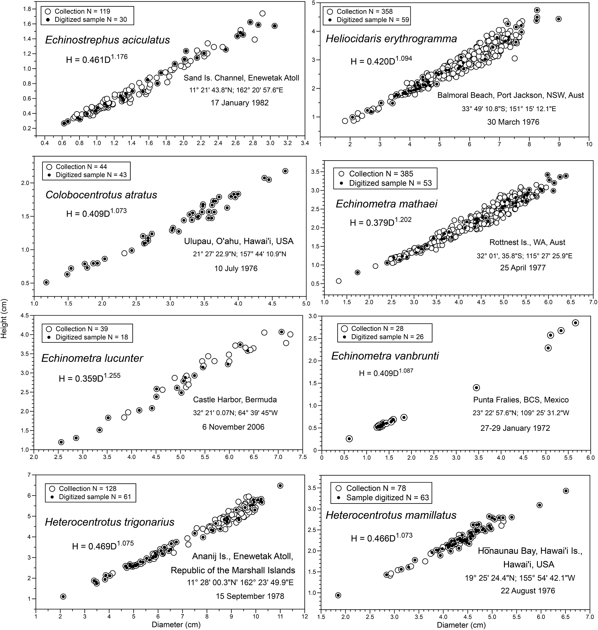
Eight sea urchin species were selected in the Family Echinometridae that show a range of shapes: Echinostrephus aciculatus, Colobocentrotus atratus, Heliocidaris erythrogramma, Heterocentrotus mamillatus, Heterocentrotus trigonarius, Echinometra mathaei, Echinometra lucunter, and Echinometra vanbrunti. Collections varied in size and were mostly subsampled for individuals that were studied in detail. All samples included a range of sizes (Figure 1), so height:diameter allometry is part of overall analysis. Other than E. aciculatus and H. erythrogramma, species in this study have an oblong shape but only the major diameter is used.
Samples of sea urchins used in this study showing the relationship between height (H) and diameter (D), as well as total samples collected and numbers digitized for Fourier analysis; equation for H vs. D based on ln-transformation and least-squares regression. Scales for both diameter and height are different across species because of the large size ranges: largest Heterocentrotus trigonarius has a diameter over 11 cm, whereas the largest Echinostrephus aciculatus is just over 3 cm.

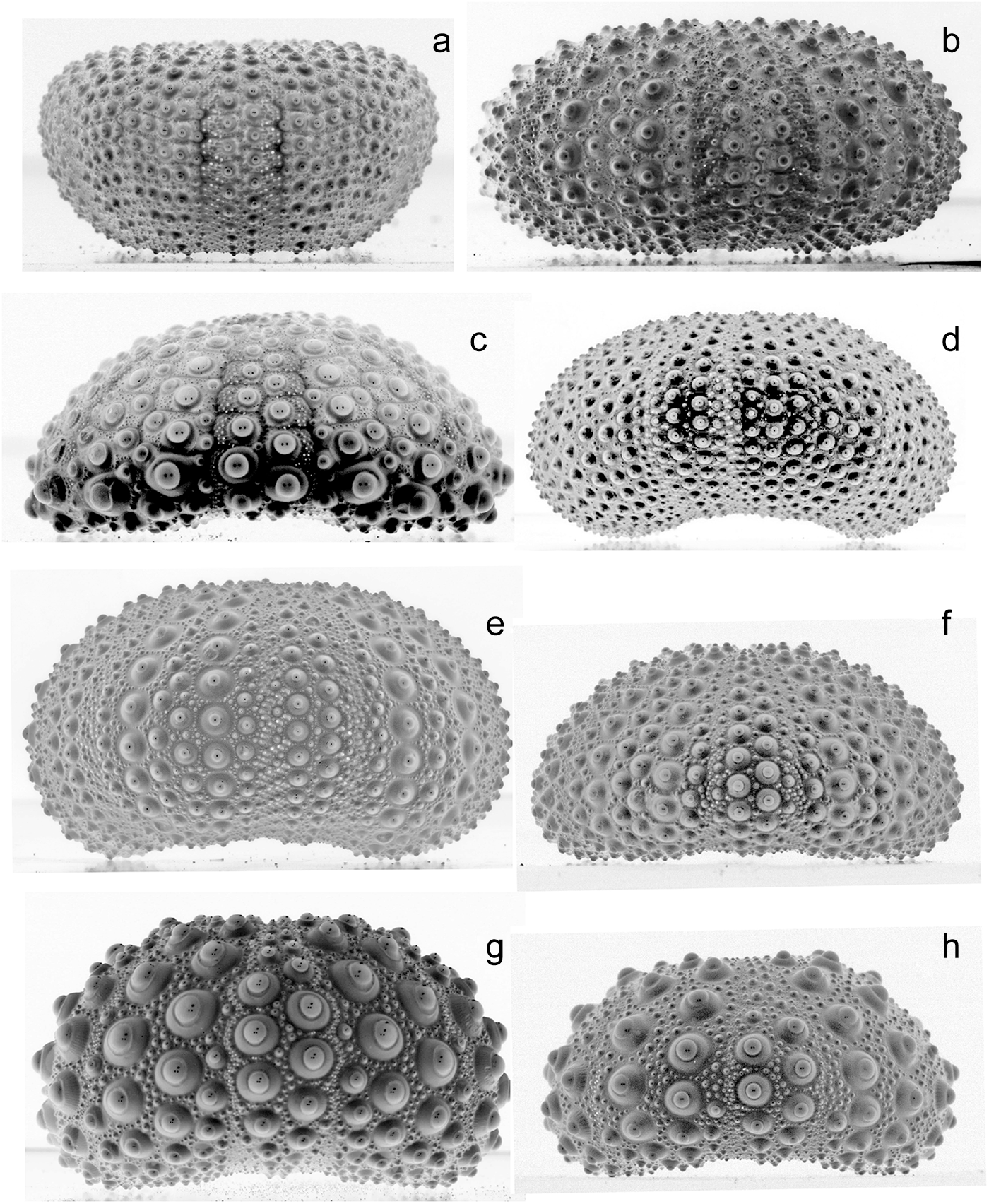
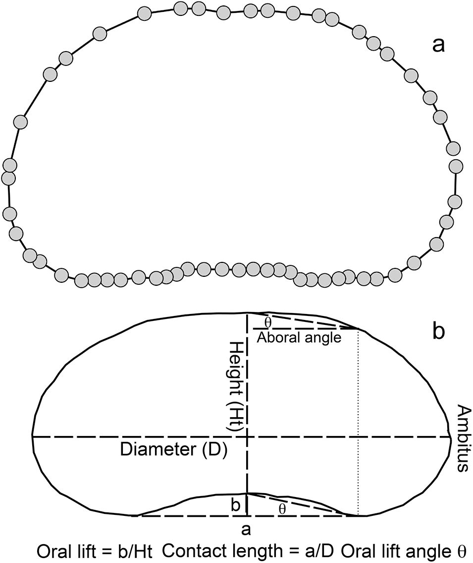
Sea urchin tests were photographed using a Canon EOS Rebel 300D camera with a 100 mm macro lens and Micro Twin Lite flash. Lens to specimen distance was adjusted so the specimen filled the frame. Images were changed to black and white negatives and adjusted to smooth shadows using Photoshop Elements (Figure 2). Images were digitized using the software PAST (Hammer and Harper, Reference Hammer and Harper2004; Hammer et al., Reference Hammer, Harper and Ryan2001) (Figure 3A) and the x–y coordinates of the path around the sea urchin image were entered into the elliptical Fourier module of PAST to generate sine and cosine coefficients for harmonics. Harmonic coefficients for all eight species were subjected to a principal components analysis.
Examples of tests of large individuals: (a) Echinostrephus aciculatus, (b) Heliocidaris erythrogramma, (c) Colobocentrotus atratus, (d) Echinometra mathaei, (e) Echinometra lucunter, (f) Echinometra vanbrunti, (g) Heterocentrotus trigonarius, (h) Heterocentrotus mamillatus.

Outlines of sea urchin tests. (a) Digitized image with x–y coordinates using PAST starting at the ambitus on the right and going around to return close to the ambitus. (b) Measurements made on a digital image that can be correlated with elliptical Fourier coefficients.

An obvious problem is how these coefficients relate to measurable attributes of a sea urchin, such as height relative to diameter, location of the ambitus relative to height, etc. Measurements on images (Figure 3B) were correlated with loadings of the principal components to interpret major harmonic coefficients and so provide insight into major shape differences within and between species.
Results
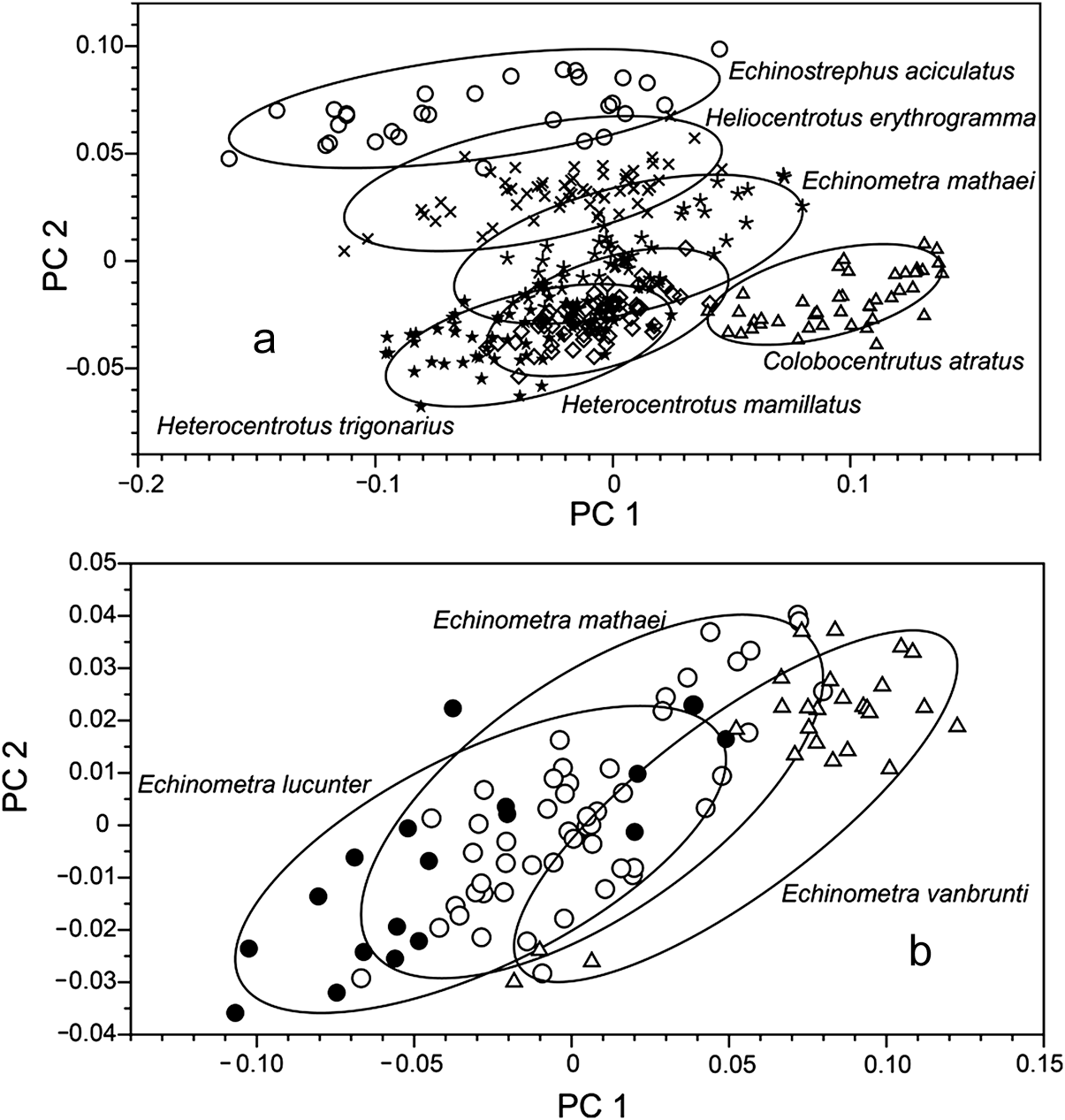
Principal components analysis showed separation of species along both axes (Figure 4A), with species with little or no oral lifting, E. aciculatus and H. erythrogramma, separated along the PC2 axis, and C. atratus separated along the PC1 axis. Because of congestion in the centre of the graph, E. mathaei, in the centre of distribution (Figure 4A), was again plotted (Figure 4B) with E. lucunter and E. vanbrunti. These three Echinometra species overlap in the PC1 and PC2 plane, even though data structures were different, particularly for E. vanbrunti, which is dominated by very small individuals.
Principal component plots with ellipses enclosing dots. (a) Species minus Echinometra lucunter and E. vanbrunti. (b) Three Echinometra species.

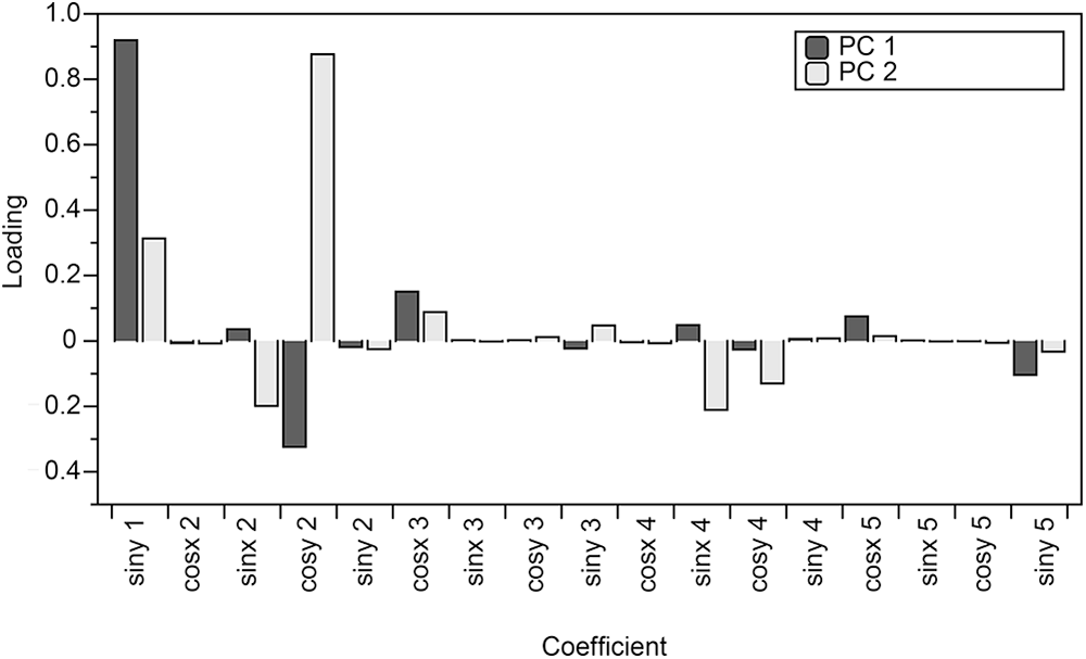
The relative importance of different Fourier coefficients of harmonics is shown by loadings of the principal components (Figure 5). For PC1, the largest loading is for siny of the first harmonic and cosy of the second harmonic. Although these are for all species combined, it is also the case for species analysed individually.
Loadings for the first two principal components.

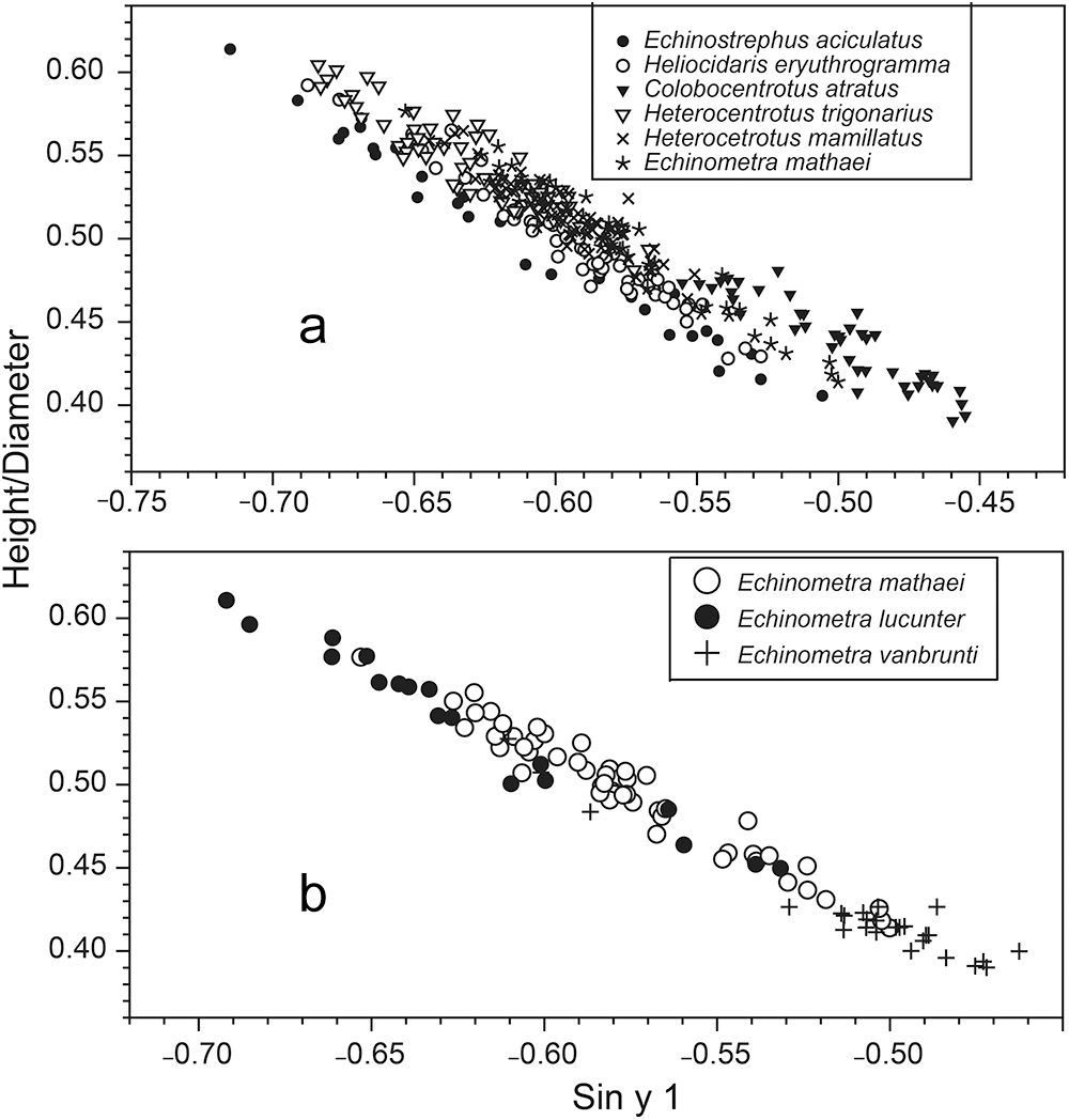
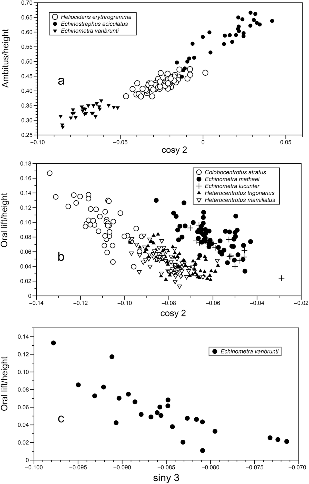
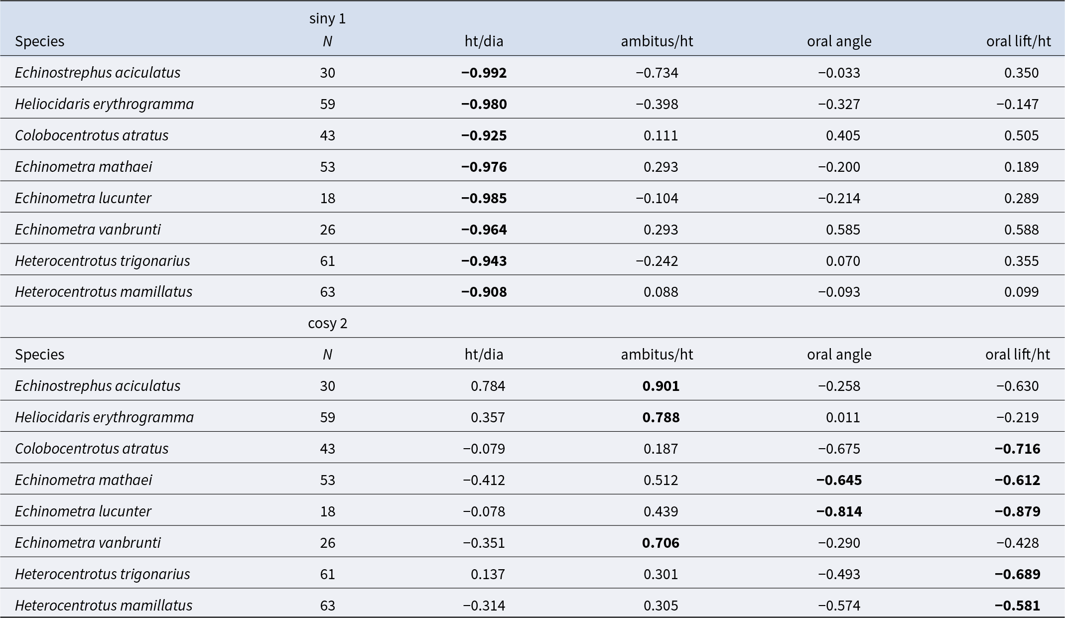
Loading coefficients for individual species were correlated with measured features (Table 1). For siny 1, all species were highly correlated with the ratio of height/diameter (Figure 6). The negative slopes show a trend from high values, where measured height can be close to 60% of measured diameter, to lows near 40%. For PC2, correlations for cosy 2 were more complex. Highest correlations for E. aciculatus, H. erythrogramma, and E. vanbrunti were with the ratio of the position of the ambitus relative to height (Figure 7A). For all other species, the highest correlations were with the lift of the oral surface relative to height (Figure 7B). Correlations with other coefficients were examined. Correlation of siny 3 mostly were similar to those for cosy 2 but showed the importance of oral lift for E. vanbrunti with a correlation coefficient of −0.81. Other loadings that were sufficiently large to be examined for several species, siny 2, siny 3, cosx 3, cosy 3, sinx 4, and cosy 4, provided no additional insights for the importance of measurements (Figure 3B). Of the measurements of images, those that were important were height/diameter, ambitus/height, and a measure of oral lift. The aboral angle did not capture an aspect of shape that is shown by elliptical Fourier analysis.
Measurements (Figure 3B) and coefficients. (a) Height/diameter vs. siny 1 for species other than Echinometra lucunter and E. vanbrunti. (b) Three Echinometra species.


Correlations between measurements (Figure 3B) and coefficients of major loadings from principal components analysis: siny of the first harmonic and cosy of the second harmonic

Discussion
All species show an increase in height relative to diameter during growth. This is shown by the allometric exponents in Figure 1 and translates into the relationship between the coefficients for siny 1 (the first harmonic) and the ratio of height:diameter. Although the slopes for all species (Figure 6A) appear very similar, line intercepts are not. Echinostrephus aciculatus data points lie below the major cloud, and points for C. atratus lie above. This probably is a reflection that not all aspects of the coefficients of siny 1 are captured by height:diameter.
The first two principal components capture 71% and 24% of the sample variance, which leaves 5% for other components. The loadings, though large for siny 1 and cosy 2, leave substantial aspects of simple shape measurements (Figure 4B) unresolved. Figure 2 shows differences in aboral flatness, and this feature apparently was not captured by the measure of aboral angle. A single value for curvature is needed. Curvature is part of the models used by Abou Chakra and Stone (Reference Abou Chakra and Stone2011), Abou Chakra et al. (Reference Abou Chakra, Lovric and Stone2017), Baron (Reference Baron1991), and Ellers (Reference Ellers1993), but I did not find a way to adapt their curvature approaches to the current study. With more work, however, I think that it can be done.
Figure 4 is a morphospace in the sense of Budd (Reference Budd2021), Gerber (Reference Gerber2016) and Mitteroecker and Huttegger (Reference Mitteroecker and Huttegger2009) with separation of species along both principal component axes. Extremes are Echinostrephus aciculatus in the upper right (Figure 4A) and C. atratus lower and to the right. The major shape difference between these two species is the relative position of the ambitus and oral lift. The ambitus is high for E. aciculatus and low for C. atratus. Also, E. aciculatus shows little or no oral lift compared with C. atratus. Table 1, however, does not indicate ambitus/height to have a high correlation coefficient with cosy 2 for C. atratus. The explanation is that the correlations are based on the individual samples and so do not include the ontogenetic change in ambitus/height allometry.
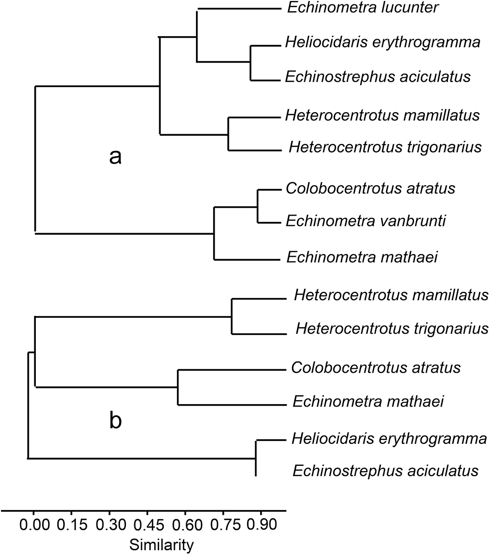
The separation of species in Figure 4 can be explored using the means of principal component values for all species. Correlations of mean PC values based on the first four principal components using PAST are linked as similarities. First with all species (Figure 8A) and then excluding those species with small sample sizes and, in the case of E. vanbrunti, with most of the sample represented by small individuals (Figure 1). The linkage of E. lucunter with H. erythrogramma and E. aciculatus (Figure 8A) is surprising given their separation in Figure 4 but may reflect small sample size of E. lucunter. Similarity of C. atratus with E. vanbrunti may hinge on shape (Figure 2C and F). Eliminating E. lucunter and E. vanbrunti from analysis (Figure 8B) provides similarities that link C. atratus with E. mathaei, H. mamillatus with H. trigonarius and H. erythrogramma with E. aciculatus. The links have similarities with the cladistic analysis given by Kinjo et al. (Reference Kinjo, Shirayama, Wada, Heinzeller and Nebelsick2004), who suggest three clades: (1) Heterocentrotus, Colobocentrotus, and Echinometra; (2) Heliocidaris and Anthocidaris; and (3) Echinostrephus.
Similarity measures based on correlations of means of principal components 1–4. (a) All species linking Echinometra species with various other species. (b) Similarities without Echinometra lucunter and E. vanbrunti.

The relationship between shape and physical forces of water has been a basis of various studies (Denny and Gaylord, Reference Denny and Gaylord1996; Telford, Reference Telford1985). These studies, however, do not include the oral lift in calculations or experiments. The oral lift would change the distribution of forces from wave shock as well as the response to lateral water flow. Incorporating oral lift may be important in understanding the dynamics and energetics of shape, and I think it deserves inclusion in models and experiments.
Future work could include examination of environmental factors associated with shape of individual species. E. mathaei, for example, excavates and lives in cavities in locations of moderate to high water motion, but also lives outside cavities in more sheltered environments. Related to this is the question of how shape and growth are related, which possibly are included in the differences between major and minor diameters. This would move to a 3-D Fourier analysis. Environmental issues may be best addressed using species with large collections spanning many habitats, such as Strongylocentrotus purpuratus (Ebert, Reference Ebert2010; Ebert et al., Reference Ebert, L. Barr and Bodkin2018).
Finally, the approach of Raup (Reference Raup1966) on modelling mollusc shape with a small number of parameters is interesting and worth exploring for sea urchins. A problem is selecting an appropriate model with a small number of parameters that includes oral lift. Shape models that start with water droplets (e.g. Ellers, Reference Ellers1993) or soap bubbles (Abou Chakra, Reference Abou Chakra2010) will not do this. A cardioid using x–y coordinates may work, and ideally, this would include the flat area at the top of the lift, but this may not be necessary.
Acknowledgements
Colleagues and assistants who were important in field work are: D. Bartley and T. Turk (Enewetak); J. Harrison III (Hawai’i); M. Moran and S. Franklin (NSW, Australia); R. Black and P. Chalmer (W. Australia); M. Russell and A. Bodnar (Bermuda); D. Dexter and S. Adair (Baja California, Mexico). PAST was suggested to me by B. Sidlauskas.
Funding.
Funding for various parts of this work was from the US National Science Foundation OCE 75-10442; OCE 75-10442 A01; OCE-8401415, US Department of Energy (DOE) to the University of Hawaii, and the Bermuda Institute of Ocean Sciences.
Competing interests
The author declares there is none.
Data availability.
From the author on request.