


1 Introduction
Compressible flows commonly exhibit richer physics than observed in the incompressible regime. In particular, compressibility fundamentally affects the physics of laminar–turbulent transition. High speeds alter linear growth mechanisms and open new pathways for the amplification of infinitesimal disturbances. If the initial amplitude of disturbances is sufficiently high, their evolution deviates from linear predictions, resulting in faster growth and the potential of earlier breakdown to turbulence. The study of the particular, optimal disturbances which translate the additional degrees of freedom provided by nonlinearity most effectively into a gain, for instance in kinetic energy, has been hitherto restricted to flows at constant density. In this work, we introduce a variational framework for the identification and analysis of general nonlinear optimal disturbances in compressible flows.
The field of laminar-turbulent transition was appreciably advanced by the understanding of the non-normality of the linearized Navier–Stokes equations which enables significant transient amplification of disturbances in the absence of exponential instability (e.g. Reddy et al. Reference Reddy, Schmid, Baggett and Henningson1993; Trefethen et al. Reference Trefethen, Trefethen, Reddy and Driscoll1993). This insight led to the development of linear transient growth theory based on non-modal stability analysis and its application in the study of a variety of shear flows (see Schmid Reference Schmid2007; Luchini & Bottaro Reference Luchini and Bottaro2014). The relevance of classical transient growth analysis derives from the view that finite-amplitude disturbances can be amplified to levels sufficiently high to induce the amplification of secondary instabilities (see e.g. Hack & Zaki Reference Hack and Zaki2014). For many parallel shear flows, the optimal disturbances which maximize transient growth are found to be streamwise independent (Gustavsson Reference Gustavsson1991) and to generate streamwise streaks by means of the lift-up mechanism (Butler & Farrell Reference Butler and Farrell1992). If the base flow is non-parallel, the effectiveness of lift-up may be enhanced by interaction with the Orr mechanism (Cherubini et al. Reference Cherubini, Robinet, Bottaro and De Palma2010; Monokrousos et al. Reference Monokrousos, Åkervik, Brandt and Henningson2010; Hack & Moin Reference Hack and Moin2017), which describes the second pathway for the transient amplification of disturbances in shear flows and amplifies disturbances of finite streamwise wavelength by tilting via the mean shear.
In various settings, the sequential consideration of linear transient growth theory and linear secondary instability analysis reveals the main features of laminar–turbulent transition (see e.g. Reddy et al. Reference Reddy, Schmid, Baggett and Henningson1998; Andersson et al. Reference Andersson, Brandt, Bottaro and Henningson2001; Roizner, Karp & Cohen Reference Roizner, Karp and Cohen2016). As a whole, the transition process is nonetheless strongly nonlinear, with the nonlinear terms of the governing equations redistributing energy between different scales of the disturbances. Specifically, nonlinear interactions have been found to fundamentally affect the generation of streaks in transient growth, including the observed fluid structures and the maximal energy gain (Pringle & Kerswell Reference Pringle and Kerswell2010). A variational approach was applied in the identification of optimal disturbances in miscellaneous incompressible flow configurations, including plane Couette flow (Monokrousos et al. Reference Monokrousos, Bottaro, Brandt, Vita and Henningson2011; Rabin, Caulfield & Kerswell Reference Rabin, Caulfield and Kerswell2012; Eaves & Caulfield Reference Eaves and Caulfield2015), pipe flow (Pringle, Willis & Kerswell Reference Pringle, Willis and Kerswell2012), boundary layers (Cherubini et al. Reference Cherubini, Robinet, Bottaro and De Palma2010, Reference Cherubini, Palma, Robinet and Bottaro2011) and plane Poiseuille flow (Farano et al. Reference Farano, Cherubini, Robinet and Palma2015). The variational method has also been extended to identify exact coherent states (Olvera & Kerswell Reference Olvera and Kerswell2017) and heteroclinic connections between turbulent equilibrium states (Farano et al. Reference Farano, Cherubini, Robinet, De Palma and Schneider2019).
The variational method is commonly implemented in terms of a Lagrange function whose stationary points identify extrema of the objective functional (e.g. Kerswell Reference Kerswell2018). In this setting, the adjoint variables are formally introduced as Lagrange multipliers which enforce the governing equations as constraints. A variety of possible choices exist for the objective functional, including the disturbance kinetic energy at a given time horizon (Pringle & Kerswell Reference Pringle and Kerswell2010) and the time-averaged dissipation (Monokrousos et al. Reference Monokrousos, Bottaro, Brandt, Vita and Henningson2011; Eaves & Caulfield Reference Eaves and Caulfield2015).
For sufficiently large time horizons, the variational nonlinear optimization method can identify the disturbance field which triggers transition to turbulence at minimal initial energy, sometimes referred to as the minimal seed of turbulence (Pringle et al. Reference Pringle, Willis and Kerswell2012; Kerswell Reference Kerswell2018). This interpretation of the minimal seed, which is also used in the present work, differs to some extent from that introduced by Cherubini et al. (Reference Cherubini, Palma, Robinet and Bottaro2011), who defined the minimal seed as a basic building block of the nonlinear optimal solution, and more specifically as the smallest flow structure that causes energy growth over short times.
More recently, Rigas, Sipp & Colonius (Reference Rigas, Sipp and Colonius2020) studied nonlinear optimal disturbances in the frequency domain by extending resolvent analysis (Jovanovic & Bamieh Reference Jovanovic and Bamieh2005; McKeon & Sharma Reference McKeon and Sharma2010) to the nonlinear setting. The application to a transitional boundary layer reproduced the mechanisms of canonical breakdown scenarios identified in Hack & Moin (Reference Hack and Moin2018).
Nonlinear optimal disturbances and minimal seeds in particular are spatially localized and comprise a multitude of wavenumbers and frequencies. As such, they qualitatively differ from the monochromatic solutions to the classical linear transient growth problem. The evolution of nonlinear optimal disturbances often begins with amplification via the Orr mechanism, followed by oblique nonlinear interactions and lift-up. This amalgamation of multiple growth mechanisms allows nonlinear optimal initial conditions to attain considerably higher amplification than observed in linear transient growth (Pringle & Kerswell Reference Pringle and Kerswell2010). From an applications point of view, nonlinear optimal disturbances and minimal seeds can be understood as an upper bound in terms of the effectiveness of inducing transition to turbulence. In a general setting with broadband excitation of disturbances inside a shear layer, perturbations which conform to these solutions can thus be expected to rapidly advance the flow towards a turbulent state.
Although the study of general nonlinear optimal disturbances has received considerable attention in recent years, these analyses have been limited to incompressible flows. Transition to turbulence is nonetheless of particular practical relevance in various settings which exhibit non-negligible compressibility effects. Our study implements the first analysis of general nonlinear optimal disturbances in compressible flows. Herein, we derive a variational framework based on the compressible Navier–Stokes equations in conserved variables. The algorithm is applied in the study of the amplification of perturbations in compressible pipe flow at various Mach numbers.
2 Variational method for compressible flow
In the following, we introduce a formulation enabling the identification of general nonlinear optimal disturbances in compressible flows. The framework is generic and compatible with a wide range of objective functionals. Within the scope of this study, we nonetheless restrict ourselves to the optimization of the kinetic energy of the computed disturbances. For the pipe setting considered within this work, all quantities are non-dimensionalized by the centreline speed of sound, the centreline density and the pipe diameter.
The governing equations for a compressible Newtonian fluid in the conserved state vector  $\boldsymbol{q}=(\unicode[STIX]{x1D70C},m_{i},e)^{\mathsf{T}}$ are
 $$\begin{eqnarray}\displaystyle & \displaystyle \frac{\unicode[STIX]{x2202}\unicode[STIX]{x1D70C}}{\unicode[STIX]{x2202}t}+\frac{\unicode[STIX]{x2202}m_{j}}{\unicode[STIX]{x2202}x_{j}}=0, & \displaystyle\end{eqnarray}$$
 $$\begin{eqnarray}\displaystyle & \displaystyle \frac{\unicode[STIX]{x2202}m_{i}}{\unicode[STIX]{x2202}t}+\frac{\unicode[STIX]{x2202}m_{i}m_{j}/\unicode[STIX]{x1D70C}}{\unicode[STIX]{x2202}x_{j}}=-\frac{\unicode[STIX]{x2202}p}{\unicode[STIX]{x2202}x_{i}}+\frac{\unicode[STIX]{x2202}}{\unicode[STIX]{x2202}x_{j}}\frac{\unicode[STIX]{x1D707}}{Re}\left(\frac{\unicode[STIX]{x2202}m_{i}/\unicode[STIX]{x1D70C}}{\unicode[STIX]{x2202}x_{j}}+\frac{\unicode[STIX]{x2202}m_{j}/\unicode[STIX]{x1D70C}}{\unicode[STIX]{x2202}x_{i}}-\frac{2}{3}\frac{\unicode[STIX]{x2202}m_{k}/\unicode[STIX]{x1D70C}}{\unicode[STIX]{x2202}x_{k}}\unicode[STIX]{x1D6FF}_{ij}\right), & \displaystyle\end{eqnarray}$$
 $$\begin{eqnarray}\displaystyle \frac{\unicode[STIX]{x2202}e}{\unicode[STIX]{x2202}t}+\frac{\unicode[STIX]{x2202}(e+p)m_{j}/\unicode[STIX]{x1D70C}}{\unicode[STIX]{x2202}x_{j}} & = & \displaystyle \frac{\unicode[STIX]{x2202}}{\unicode[STIX]{x2202}x_{j}}\frac{\unicode[STIX]{x1D707}}{Re\;Pr}\frac{\unicode[STIX]{x2202}\left(e-{\displaystyle \frac{1}{2}}m_{i}m_{i}/\unicode[STIX]{x1D70C}\right){\displaystyle \frac{\unicode[STIX]{x1D6FE}}{\unicode[STIX]{x1D70C}}}}{\unicode[STIX]{x2202}x_{j}}\nonumber\\ \displaystyle & & \displaystyle +\,\frac{\unicode[STIX]{x2202}}{\unicode[STIX]{x2202}x_{j}}\frac{\unicode[STIX]{x1D707}}{Re}\left(m_{k}/\unicode[STIX]{x1D70C}\left(\frac{\unicode[STIX]{x2202}m_{k}/\unicode[STIX]{x1D70C}}{\unicode[STIX]{x2202}x_{j}}+\frac{\unicode[STIX]{x2202}m_{j}/\unicode[STIX]{x1D70C}}{\unicode[STIX]{x2202}x_{k}}-\frac{2}{3}\frac{\unicode[STIX]{x2202}m_{l}/\unicode[STIX]{x1D70C}}{\unicode[STIX]{x2202}x_{l}}\unicode[STIX]{x1D6FF}_{jk}\right)\right),\nonumber\\ \displaystyle & & \displaystyle\end{eqnarray}$$
where  $i,j,k\in \{1,2,3\}$ and
 $m_{j}=\unicode[STIX]{x1D70C}u_{j}$ are the mass fluxes aligned with the Cartesian components of the fluid velocity vector,
 $u_{j}$. Further,
 $e=p/(\unicode[STIX]{x1D6FE}-1)+1/2\unicode[STIX]{x1D70C}u_{i}u_{i}$ is the total energy,
 $\unicode[STIX]{x1D70C}$ is density,
 $p$ denotes pressure,
 $\unicode[STIX]{x1D707}$ the molecular viscosity,
 $\unicode[STIX]{x1D6FE}=1.4$ the ratio of the specific heats,
 $Re$ is the Reynolds number based on the speed of sound,
 $a=\sqrt{\unicode[STIX]{x1D6FE}p/\unicode[STIX]{x1D70C}}$, and
 $Pr$ is the Prandtl number which takes a constant value of 0.70 within this study. The dependence of the viscosity,
 $\unicode[STIX]{x1D707}$, on the temperature,
 $T$, is modelled using a power law of the form
 $\unicode[STIX]{x1D707}=\left(\left(\unicode[STIX]{x1D6FE}-1\right)T\right)^{n}$ with
 $n=0.7$. The governing equations are closed by the equation of state for an ideal gas:
 $$\begin{eqnarray}p=\frac{\unicode[STIX]{x1D6FE}-1}{\unicode[STIX]{x1D6FE}}\unicode[STIX]{x1D70C}T.\end{eqnarray}$$
We note that the above equations describe the evolution of the Cartesian components of the velocity and mass flux vectors, in alignment with the quantities that are being solved within our computational framework. The cylindrical pipe setting is accounted for via metric factors in a discretely consistent curvilinear discretization which satisfies geometric conservation properties (Thomas & Lombard Reference Thomas and Lombard1979) and thus enables a highly accurate treatment of a variety of configurations, including pipes.
Without loss of generality, we separate the flow variables into a steady base state, marked by an overbar, and a perturbation component, denoted by a prime,  $\unicode[STIX]{x1D712}=\overline{\unicode[STIX]{x1D712}}+\unicode[STIX]{x1D712}^{\prime }$. Introduction into (2.1)–(2.3) yields the five equations
 $$\begin{eqnarray}\displaystyle \text{C}0: & & \displaystyle \frac{\unicode[STIX]{x2202}\unicode[STIX]{x1D70C}^{\prime }}{\unicode[STIX]{x2202}t}+\frac{\unicode[STIX]{x2202}(\overline{m}_{j}+m_{j}^{\prime })}{\unicode[STIX]{x2202}x_{j}}=0,\end{eqnarray}$$
 $$\begin{eqnarray}\displaystyle \text{C}i: & & \displaystyle \frac{\unicode[STIX]{x2202}m_{i}^{\prime }}{\unicode[STIX]{x2202}t}+\frac{\unicode[STIX]{x2202}}{\unicode[STIX]{x2202}x_{j}}\frac{(\overline{m}_{i}+m_{i}^{\prime })(\overline{m}_{j}+m_{j}^{\prime })}{\overline{\unicode[STIX]{x1D70C}}+\unicode[STIX]{x1D70C}^{\prime }}+\frac{\unicode[STIX]{x2202}(\overline{p}+p^{\prime })}{\unicode[STIX]{x2202}x_{i}}\nonumber\\ \displaystyle & & \displaystyle \qquad \quad -\,\frac{\unicode[STIX]{x2202}}{\unicode[STIX]{x2202}x_{j}}\frac{\unicode[STIX]{x1D707}}{Re}\left(\frac{\unicode[STIX]{x2202}}{\unicode[STIX]{x2202}x_{j}}\frac{\overline{m}_{i}+m_{i}^{\prime }}{\overline{\unicode[STIX]{x1D70C}}+\unicode[STIX]{x1D70C}^{\prime }}+\frac{\unicode[STIX]{x2202}}{\unicode[STIX]{x2202}x_{i}}\frac{\overline{m}_{j}+m_{j}^{\prime }}{\overline{\unicode[STIX]{x1D70C}}+\unicode[STIX]{x1D70C}^{\prime }}-\frac{2}{3}\frac{\unicode[STIX]{x2202}}{\unicode[STIX]{x2202}x_{k}}\frac{\overline{m}_{k}+m_{k}^{\prime }}{\overline{\unicode[STIX]{x1D70C}}+\unicode[STIX]{x1D70C}^{\prime }}\unicode[STIX]{x1D6FF}_{ij}\right)=0,\nonumber\\ \displaystyle & & \displaystyle\end{eqnarray}$$
 $$\begin{eqnarray}\displaystyle \text{C}4: & & \displaystyle \frac{\unicode[STIX]{x2202}e^{\prime }}{\unicode[STIX]{x2202}t}+\frac{\unicode[STIX]{x2202}}{\unicode[STIX]{x2202}x_{j}}\frac{(\overline{e}+e^{\prime }+\overline{p}+p^{\prime })(\overline{m}_{j}+m_{j}^{\prime })}{\overline{\unicode[STIX]{x1D70C}}+\unicode[STIX]{x1D70C}^{\prime }}\nonumber\\ \displaystyle & & \displaystyle \qquad \quad -\,\frac{\unicode[STIX]{x2202}}{\unicode[STIX]{x2202}x_{j}}\frac{\unicode[STIX]{x1D707}}{Re\;Pr}\frac{\unicode[STIX]{x2202}}{\unicode[STIX]{x2202}x_{j}}\frac{(\overline{e}+e^{\prime }-(1/2)(\overline{m}_{i}+m_{i}^{\prime })(\overline{m}_{i}+m_{i}^{\prime })/(\overline{\unicode[STIX]{x1D70C}}+\unicode[STIX]{x1D70C}^{\prime }))\unicode[STIX]{x1D6FE}}{\overline{\unicode[STIX]{x1D70C}}+\unicode[STIX]{x1D70C}^{\prime }}\nonumber\\ \displaystyle & & \displaystyle \qquad \quad -\,\frac{\unicode[STIX]{x2202}}{\unicode[STIX]{x2202}x_{j}}\frac{\unicode[STIX]{x1D707}}{Re}\left(\frac{\overline{m}_{k}+m_{k}^{\prime }}{\overline{\unicode[STIX]{x1D70C}}+\unicode[STIX]{x1D70C}^{\prime }}\left(\frac{\unicode[STIX]{x2202}}{\unicode[STIX]{x2202}x_{j}}\frac{\overline{m}_{k}+m_{k}^{\prime }}{\overline{\unicode[STIX]{x1D70C}}+\unicode[STIX]{x1D70C}^{\prime }}+\frac{\unicode[STIX]{x2202}}{\unicode[STIX]{x2202}x_{k}}\frac{\overline{m}_{j}+m_{j}^{\prime }}{\overline{\unicode[STIX]{x1D70C}}+\unicode[STIX]{x1D70C}^{\prime }}\right)\right)\nonumber\\ \displaystyle & & \displaystyle \qquad \quad -\,\frac{\unicode[STIX]{x2202}}{\unicode[STIX]{x2202}x_{j}}\frac{\unicode[STIX]{x1D707}}{Re}\left(\frac{\overline{m}_{k}+m_{k}^{\prime }}{\overline{\unicode[STIX]{x1D70C}}+\unicode[STIX]{x1D70C}^{\prime }}\left(-\frac{2}{3}\frac{\unicode[STIX]{x2202}}{\unicode[STIX]{x2202}x_{l}}\frac{\overline{m}_{l}+m_{l}^{\prime }}{\overline{\unicode[STIX]{x1D70C}}+\unicode[STIX]{x1D70C}^{\prime }}\unicode[STIX]{x1D6FF}_{jk}\right)\right)=0,\end{eqnarray}$$
which govern perturbations in density ( $\text{C}0$), the three mass fluxes (
 $\text{C}i$) and total energy (
 $\text{C}4$).
The optimization procedure operates on the functional
 $$\begin{eqnarray}J(t)=\int _{\unicode[STIX]{x1D6FA}}\frac{m_{i}^{\prime }(t)m_{i}^{\prime }(t)}{2\overline{\unicode[STIX]{x1D70C}}}\,\text{d}V.\end{eqnarray}$$
We note that in the present setting of a state vector,  $\boldsymbol{q}=\left(\unicode[STIX]{x1D70C},m_{i},e\right)^{\mathsf{T}}$, there exists no positive definite norm that would yield a direct equivalent to the kinetic energy commonly considered in the incompressible regime. Since
 $m_{i}^{\prime }=\overline{\unicode[STIX]{x1D70C}}u_{i}^{\prime }+\unicode[STIX]{x1D70C}^{\prime }\overline{u}_{i}+\unicode[STIX]{x1D70C}^{\prime }u_{i}^{\prime }$, with
 $\unicode[STIX]{x1D70C}^{\prime }$ an independent variable in the kernel of
 $J(t)$, the maximization of (2.8) effectively maximizes the kinetic energy of the perturbations,
 $$\begin{eqnarray}E(t)=\frac{\overline{\unicode[STIX]{x1D70C}}u_{i}^{\prime }\left(t\right)u_{i}^{\prime }\left(t\right)}{2}.\end{eqnarray}$$
The objective of identifying the initial perturbations whose evolution during the finite time interval  $t_{1}$ results in the highest gain in perturbation kinetic energy, is hence represented by maximizing the objective functional
 $$\begin{eqnarray}{\mathcal{J}}=J(t_{1}).\end{eqnarray}$$
Naturally, we wish to prescribe the initial amplitude of the perturbations at the initial time  $t=0$, and we require the computed perturbations to be solutions to the compressible Navier–Stokes equations (2.5)–(2.7). The resulting constrained optimization problem may be expressed as the Lagrangian
 $$\begin{eqnarray}\displaystyle {\mathcal{L}} & = & \displaystyle {\mathcal{L}}(\unicode[STIX]{x1D70C}^{\prime },m_{i}^{\prime },e^{\prime },\unicode[STIX]{x1D702},\unicode[STIX]{x1D706}_{i},\unicode[STIX]{x1D703},\unicode[STIX]{x1D6FC};E_{0},t_{1})={\mathcal{J}}-\unicode[STIX]{x1D6FC}(J(0)-E_{0})\nonumber\\ \displaystyle & & \displaystyle -\,\int _{0}^{t_{1}}\langle \unicode[STIX]{x1D702},\text{C}0\rangle \,\text{d}t-\int _{0}^{t_{1}}\langle \unicode[STIX]{x1D706}_{i},\text{C}i\rangle \,\text{d}t-\int _{0}^{t_{1}}\langle \unicode[STIX]{x1D703},\text{C}4\rangle \,\text{d}t,\end{eqnarray}$$
whose stationary points identify the optimal solution. The integral inner product in (2.11) is defined as
 $$\begin{eqnarray}\langle a,b\rangle =\int _{\unicode[STIX]{x1D6FA}}a^{\mathsf{H}}b\,\text{d}V.\end{eqnarray}$$
The Lagrange multipliers  $\unicode[STIX]{x1D702}$,
 $\unicode[STIX]{x1D706}_{i}$ and
 $\unicode[STIX]{x1D703}$ can be interpreted as the adjoint density, mass flux and energy perturbations. The stationary points of the Lagrangian are found by setting its first variations with respect to each multiplier to zero. For
 $\unicode[STIX]{x1D702},$
 $\unicode[STIX]{x1D706}_{i}$,
 $\unicode[STIX]{x1D703}$ and
 $\unicode[STIX]{x1D6FC}$, doing so recovers the direct Navier–Stokes equations, C0–C4, as well as the constraint on the initial condition
 $$\begin{eqnarray}\frac{\unicode[STIX]{x1D6FF}{\mathcal{L}}}{\unicode[STIX]{x1D6FF}\unicode[STIX]{x1D6FC}}=J(0)-E_{0}=0.\end{eqnarray}$$
Setting the first variation of the Lagrangian with respect to perturbations in density, mass fluxes and total energy to zero yields the following set of adjoint equations, which must be satisfied within the computational domain,
 $$\begin{eqnarray}\displaystyle \frac{\unicode[STIX]{x1D6FF}{\mathcal{L}}}{\unicode[STIX]{x1D6FF}\unicode[STIX]{x1D70C}^{\prime }} & = & \displaystyle \unicode[STIX]{x1D702}_{t}-\frac{m_{i}m_{j}}{\unicode[STIX]{x1D70C}^{2}}(\unicode[STIX]{x1D706}_{i})_{x_{j}}+\frac{(\unicode[STIX]{x1D6FE}-1)m_{j}m_{j}}{2\unicode[STIX]{x1D70C}^{2}}(\unicode[STIX]{x1D706}_{i})_{x_{i}}-\left[\unicode[STIX]{x1D6FE}e-(\unicode[STIX]{x1D6FE}-1)\frac{m_{i}m_{i}}{\unicode[STIX]{x1D70C}}\right]\frac{m_{j}}{\unicode[STIX]{x1D70C}^{2}}\unicode[STIX]{x1D703}_{x_{j}}\nonumber\\ \displaystyle & & \displaystyle -\,\frac{\unicode[STIX]{x1D6FE}}{\unicode[STIX]{x1D70C}^{2}Re\;Pr}\left(e-\frac{m_{i}m_{i}}{\unicode[STIX]{x1D70C}}\right)\left(\unicode[STIX]{x1D703}_{x_{j}}\unicode[STIX]{x1D707}\right)_{x_{j}}\nonumber\\ \displaystyle & & \displaystyle -\,\frac{1}{\unicode[STIX]{x1D70C}^{2}Re}\left(m_{i}\left[\unicode[STIX]{x1D707}(\unicode[STIX]{x1D706}_{i})_{x_{j}}+\unicode[STIX]{x1D707}\unicode[STIX]{x1D703}_{x_{i}}\frac{m_{j}}{\unicode[STIX]{x1D70C}}\right]_{x_{j}}+m_{j}\left[\unicode[STIX]{x1D707}(\unicode[STIX]{x1D706}_{i})_{x_{j}}+\unicode[STIX]{x1D707}\unicode[STIX]{x1D703}_{x_{i}}\frac{m_{j}}{\unicode[STIX]{x1D70C}}\right]_{x_{i}}\right.\nonumber\\ \displaystyle & & \displaystyle \left.-\,\frac{2}{3}m_{j}\left[\unicode[STIX]{x1D707}(\unicode[STIX]{x1D706}_{i})_{x_{i}}+\unicode[STIX]{x1D707}\unicode[STIX]{x1D703}_{x_{i}}\frac{m_{i}}{\unicode[STIX]{x1D70C}}\right]_{x_{j}}-\unicode[STIX]{x1D707}m_{j}\unicode[STIX]{x1D703}_{x_{i}}\unicode[STIX]{x1D70F}_{ij}\right)-\frac{1}{Re}\frac{\unicode[STIX]{x2202}\unicode[STIX]{x1D707}}{\unicode[STIX]{x2202}\unicode[STIX]{x1D70C}^{\prime }}\left((\unicode[STIX]{x1D706}_{i})_{x_{j}}\unicode[STIX]{x1D70F}_{ij}+\unicode[STIX]{x1D703}_{x_{j}}\frac{m_{i}}{\unicode[STIX]{x1D70C}}\unicode[STIX]{x1D70F}_{ij}\right)=0,\nonumber\\ \displaystyle & & \displaystyle\end{eqnarray}$$
 $$\begin{eqnarray}\displaystyle \frac{\unicode[STIX]{x1D6FF}{\mathcal{L}}}{\unicode[STIX]{x1D6FF}m_{i}^{\prime }} & = & \displaystyle (\unicode[STIX]{x1D706}_{i})_{t}+\unicode[STIX]{x1D702}_{x_{i}}+\frac{m_{j}}{\unicode[STIX]{x1D70C}}(\unicode[STIX]{x1D706}_{j})_{x_{i}}-\frac{m_{i}}{\unicode[STIX]{x1D70C}}(\unicode[STIX]{x1D6FE}-1)(\unicode[STIX]{x1D706}_{j})_{x_{j}}+\frac{m_{j}}{\unicode[STIX]{x1D70C}}(\unicode[STIX]{x1D706}_{i})_{x_{j}}\nonumber\\ \displaystyle & & \displaystyle +\,\frac{\unicode[STIX]{x1D6FE}e-1/2(\unicode[STIX]{x1D6FE}-1)m_{j}m_{j}/\unicode[STIX]{x1D70C}}{\unicode[STIX]{x1D70C}}\unicode[STIX]{x1D703}_{x_{i}}-\frac{m_{j}m_{i}}{\unicode[STIX]{x1D70C}^{2}}(\unicode[STIX]{x1D6FE}-1)\unicode[STIX]{x1D703}_{x_{j}}-\frac{\unicode[STIX]{x1D6FE}m_{i}}{\unicode[STIX]{x1D70C}^{2}Re\;Pr}\left(\unicode[STIX]{x1D703}_{x_{j}}\unicode[STIX]{x1D707}\right)_{x_{j}}\nonumber\\ \displaystyle & & \displaystyle +\,\frac{1}{\unicode[STIX]{x1D70C}Re}\left(\left[\unicode[STIX]{x1D707}(\unicode[STIX]{x1D706}_{j})_{x_{i}}+\unicode[STIX]{x1D707}\unicode[STIX]{x1D703}_{x_{j}}\frac{m_{i}}{\unicode[STIX]{x1D70C}}\right]_{x_{j}}+\left[\unicode[STIX]{x1D707}(\unicode[STIX]{x1D706}_{i})_{x_{j}}+\unicode[STIX]{x1D707}\unicode[STIX]{x1D703}_{x_{i}}\frac{m_{j}}{\unicode[STIX]{x1D70C}}\right]_{x_{j}}\right.\nonumber\\ \displaystyle & & \displaystyle \left.-\,\frac{2}{3}\left[\unicode[STIX]{x1D707}(\unicode[STIX]{x1D706}_{j})_{x_{j}}+\unicode[STIX]{x1D707}\unicode[STIX]{x1D703}_{x_{j}}\frac{m_{j}}{\unicode[STIX]{x1D70C}}\right]_{x_{i}}-\unicode[STIX]{x1D707}\unicode[STIX]{x1D703}_{x_{j}}\unicode[STIX]{x1D70F}_{ij}\right)-\frac{1}{Re}\frac{\unicode[STIX]{x2202}\unicode[STIX]{x1D707}}{\unicode[STIX]{x2202}m_{i}^{\prime }}\left[(\unicode[STIX]{x1D706}_{k})_{x_{j}}\unicode[STIX]{x1D70F}_{kj}+\unicode[STIX]{x1D703}_{x_{j}}\frac{m_{k}}{\unicode[STIX]{x1D70C}}\unicode[STIX]{x1D70F}_{kj}\right]=0,\nonumber\\ \displaystyle & & \displaystyle\end{eqnarray}$$
 $$\begin{eqnarray}\displaystyle \frac{\unicode[STIX]{x1D6FF}{\mathcal{L}}}{\unicode[STIX]{x1D6FF}e^{\prime }} & = & \displaystyle \unicode[STIX]{x1D703}_{t}+\left(\unicode[STIX]{x1D706}_{i}\right)_{x_{i}}(\unicode[STIX]{x1D6FE}-1)+\unicode[STIX]{x1D6FE}\unicode[STIX]{x1D703}_{x_{j}}\frac{m_{j}}{\unicode[STIX]{x1D70C}}\nonumber\\ \displaystyle & & \displaystyle +\,\left(\unicode[STIX]{x1D703}_{x_{j}}\frac{\unicode[STIX]{x1D707}}{Re\;Pr}\right)_{x_{j}}\frac{\unicode[STIX]{x1D6FE}}{\unicode[STIX]{x1D70C}}-\frac{1}{Re}\frac{\unicode[STIX]{x2202}\unicode[STIX]{x1D707}}{\unicode[STIX]{x2202}e^{\prime }}\left(\left(\unicode[STIX]{x1D706}_{i}\right)_{x_{j}}\unicode[STIX]{x1D70F}_{ij}+\frac{m_{k}}{\unicode[STIX]{x1D70C}}\unicode[STIX]{x1D703}_{x_{j}}\unicode[STIX]{x1D70F}_{ij}\right)=0.\end{eqnarray}$$
Here,  $\unicode[STIX]{x1D749}$ is the shear stress tensor,
 $\unicode[STIX]{x1D70F}_{ij}\equiv \unicode[STIX]{x2202}(m_{i}/\unicode[STIX]{x1D70C})/\unicode[STIX]{x2202}x_{j}+\unicode[STIX]{x2202}(m_{j}/\unicode[STIX]{x1D70C})/\unicode[STIX]{x2202}x_{i}-2/3\unicode[STIX]{x2202}(m_{k}/\unicode[STIX]{x1D70C})/\unicode[STIX]{x2202}x_{k}\unicode[STIX]{x1D6FF}_{ij}$. The derivatives of the viscosity with respect to
 $\unicode[STIX]{x1D70C}^{\prime }$,
 $m_{i}^{\prime }$ and
 $e^{\prime }$ are
 $$\begin{eqnarray}\frac{\unicode[STIX]{x2202}\unicode[STIX]{x1D707}}{\unicode[STIX]{x2202}\unicode[STIX]{x1D70C}^{\prime }}=\unicode[STIX]{x1D6F9}\unicode[STIX]{x1D6FE}(m_{i}m_{i}\unicode[STIX]{x1D70C}^{-3}-e\unicode[STIX]{x1D70C}^{-2});\quad \frac{\unicode[STIX]{x2202}\unicode[STIX]{x1D707}}{\unicode[STIX]{x2202}m_{i}^{\prime }}=-\unicode[STIX]{x1D6F9}\unicode[STIX]{x1D6FE}m_{i}\unicode[STIX]{x1D70C}^{-2};\quad \frac{\unicode[STIX]{x2202}\unicode[STIX]{x1D707}}{\unicode[STIX]{x2202}e^{\prime }}=\unicode[STIX]{x1D6F9}\unicode[STIX]{x1D6FE}\unicode[STIX]{x1D70C}^{-1},\end{eqnarray}$$
with  $\unicode[STIX]{x1D6F9}\equiv n(\unicode[STIX]{x1D6FE}-1)[(\unicode[STIX]{x1D6FE}-1)(\unicode[STIX]{x1D6FE}/\unicode[STIX]{x1D70C})(e-\frac{1}{2}(m_{i}m_{i}/\unicode[STIX]{x1D70C}))]^{n-1}$.
Coupling conditions for the initialization of the perturbation and adjoint perturbation states are derived by setting the first variation of the Lagrange function with respect to the perturbations at initial time,  $t=0$, and the time horizon,
 $t=t_{1}$, to zero,
 $$\begin{eqnarray}\displaystyle \frac{\unicode[STIX]{x1D6FF}{\mathcal{L}}}{\unicode[STIX]{x1D6FF}\unicode[STIX]{x1D70C}^{\prime }(0)}=-\unicode[STIX]{x1D702}(0)=0;\quad \frac{\unicode[STIX]{x1D6FF}{\mathcal{L}}}{\unicode[STIX]{x1D6FF}m_{i}^{\prime }(0)}=\unicode[STIX]{x1D6FC}m_{i}^{\prime }(0)/\overline{\unicode[STIX]{x1D70C}}-\unicode[STIX]{x1D706}_{i}(0)=0;\quad \frac{\unicode[STIX]{x1D6FF}{\mathcal{L}}}{\unicode[STIX]{x1D6FF}e^{\prime }(0)}=-\unicode[STIX]{x1D703}(0)=0; & & \displaystyle \nonumber\\ \displaystyle & & \displaystyle\end{eqnarray}$$
 $$\begin{eqnarray}\displaystyle \frac{\unicode[STIX]{x1D6FF}{\mathcal{L}}}{\unicode[STIX]{x1D6FF}\unicode[STIX]{x1D70C}^{\prime }(t_{1})}=-\unicode[STIX]{x1D702}(t_{1})=0;\quad \frac{\unicode[STIX]{x1D6FF}{\mathcal{L}}}{\unicode[STIX]{x1D6FF}m_{i}^{\prime }(t_{1})}=m_{i}^{\prime }(t_{1})/\overline{\unicode[STIX]{x1D70C}}-\unicode[STIX]{x1D706}_{i}(t_{1})=0;\quad \frac{\unicode[STIX]{x1D6FF}{\mathcal{L}}}{\unicode[STIX]{x1D6FF}e^{\prime }(t_{1})}=-\unicode[STIX]{x1D703}(t_{1})=0. & & \displaystyle \nonumber\\ \displaystyle & & \displaystyle\end{eqnarray}$$
These relations do not impose compatibility constraints on the density and total energy components of the perturbation state. In our implementation, the optimization procedure thus starts with an initial guess for the optimal initial disturbances,  $\boldsymbol{q}_{0}^{\prime }=(0,m_{i}^{\prime }(0),0)^{\mathsf{T}}$. In the absence of a solution from an earlier computation for similar parameters, the procedure is initiated by applying a random field throughout the computational domain for the mass flux perturbations which is normalized so as to satisfy (2.13). In spectral terms, this implies broadband content within the range of wavenumbers supported by the computational grid. The initial condition is advanced to the target time
 $t_{1}$ by integrating the Navier–Stokes equations, providing the final state
 $\boldsymbol{q}_{1}^{\prime }=(\unicode[STIX]{x1D70C}^{\prime }(t_{1}),m_{i}^{\prime }(t_{1}),e^{\prime }(t_{1}))^{\mathsf{T}}$. Subsequently, the adjoint state vector is initialized, as described in (2.19), followed by time marching of the adjoint governing equations from
 $t=t_{1}$ to the initial time,
 $t=0$. If the objective functional attains an extremum, equation (2.18) is satisfied exactly. Otherwise, it yields an estimate for the gradient
 $\boldsymbol{g}=\unicode[STIX]{x1D6FF}{\mathcal{L}}/\unicode[STIX]{x1D6FF}m_{i}^{\prime }(0)$ which is used to update the initial condition before repeating the looping procedure as follows:
 $$\begin{eqnarray}g_{i}^{(n)}=\frac{\unicode[STIX]{x1D6FF}{\mathcal{L}}}{\unicode[STIX]{x1D6FF}m_{i}^{\prime }(0)^{(n)}}=\unicode[STIX]{x1D6FC}m_{i}^{\prime }(0)^{(n)}/\overline{\unicode[STIX]{x1D70C}}-\unicode[STIX]{x1D706}_{i}(0)^{(n)}.\end{eqnarray}$$
The initial condition is subsequently updated using steepest ascent,
 $$\begin{eqnarray}m_{i}^{\prime }(0)^{(n+1)}=m_{i}^{\prime }(0)^{(n)}+\unicode[STIX]{x1D716}(\unicode[STIX]{x1D6FC}m_{i}^{\prime }(0)^{(n)}/\overline{\unicode[STIX]{x1D70C}}-\unicode[STIX]{x1D706}_{i}(0)^{(n)}),\end{eqnarray}$$
where  $\unicode[STIX]{x1D6FC}$ is chosen to satisfy the normalization condition
 $$\begin{eqnarray}J(0)=\int _{\unicode[STIX]{x1D6FA}}\frac{m_{i}^{\prime }(0)m_{i}^{\prime }(0)}{2\overline{\unicode[STIX]{x1D70C}}}\,\text{d}V,\end{eqnarray}$$
and  $\unicode[STIX]{x1D716}$ is an adjustable parameter that regulates convergence and whose choice follows the strategy proposed by Pringle et al. (Reference Pringle, Willis and Kerswell2012). The convergence of the optimization procedure can be assessed by evaluating the normalized residual at the
 $n$th iteration:
 $$\begin{eqnarray}R_{n}=\langle g_{i}^{(n)},g_{i}^{(n)}\rangle /\langle \unicode[STIX]{x1D706}_{i}(0)^{(n)},\unicode[STIX]{x1D706}_{i}(0)^{(n)}\rangle .\end{eqnarray}$$
Within this work, the iterative procedure stops when the relative difference of the perturbation kinetic energy gain between two consecutive iterations is sufficiently small, as will be discussed in § 3.
The iterative optimization scheme based on the time integration of the forward and adjoint equations has been implemented into a compressible flow solver. The solver supports complex geometries via a consistent curvilinear formulation aligned with geometric conservation properties (Thomas & Lombard Reference Thomas and Lombard1979). The spatial discretization employs fourth-order finite differences based on summation-by-parts operators (Strand Reference Strand1994). Boundary conditions are weakly enforced via simultaneous approximation terms (Svärd & Nordström Reference Svärd and Nordström2008), supplemented by a sponge layer at the inflow and outflow of the computational domain. The boundary conditions at the inflow and outflow impose an axial pressure gradient and temperature gradient on the base flow. Homogeneous boundary conditions are imposed on the full fluctuation state vector at the inflow and outflow. Isothermal viscous boundary conditions are imposed at the pipe wall on both the base flow and the fluctuations. Time integration is facilitated by a second-order Runge–Kutta scheme, and linear checkpointing is applied in the time integration of the adjoint governing equations. The reader is referred to Flint & Hack (Reference Flint and Hack2018) for a full description of the computational framework.
A validation case of the implemented optimization procedure considers the evolution of the optimal disturbances identified with the present framework for parallel periodic pipe flow at  $Re=1750$. Consistent with the study by Pringle & Kerswell (Reference Pringle and Kerswell2010) based on the incompressible Navier–Stokes equations, the simulated axial extent of the pipe is
 $L_{x}=\unicode[STIX]{x03C0}/2$. The grid contains
 $128\times 64\times 128$ points in the axial, radial and azimuthal dimensions, respectively, and the time step is
 $\unicode[STIX]{x0394}t=10^{-4}$. The centreline convective speed is chosen to be one fifth of the speed of sound. In this setting, a base flow that is strictly periodic in the streamwise dimension is computed by supplementing the streamwise momentum and energy equations with forcing terms. At the resulting Mach number,
 $Ma=0.20$, compressibility effects are negligible and thus allow a comparison with results reported by Pringle & Kerswell (Reference Pringle and Kerswell2010). That work employed a spectral discretization based on 11 Fourier modes axially, 29 Fourier modes azimuthally and 25 modified Chebyshev polynomials in the radial dimension.
For sufficiently small initial kinetic energy,  $E_{0}=1.0\times 10^{-8}$, the contribution of the nonlinear terms becomes negligible, and the computed disturbances undergo an effectively linear evolution. Specifically, the effective absence of nonlinear interactions causes the solution to maintain the azimuthal wavenumber,
 $\unicode[STIX]{x1D6FD}=1$, imposed at the initiation of the iteration scheme. For the considered flow parameters, the scaling reported by Schmid & Henningson (Reference Schmid and Henningson1994) for the linearized incompressible governing equations predicts a gain in kinetic energy,
 $E(t)/E(0)=214.4$, after approximately
 $t_{lin,opt}=21.35$ non-dimensional time units. The results obtained with the present implementation, provided in figure 1, demonstrate excellent agreement with both the linear scaling and the result by Pringle & Kerswell (Reference Pringle and Kerswell2010).
When the initial perturbation energy is sufficiently large, here  $E_{0}=2.0\times 10^{-5}$, the optimal perturbations identified in the optimization scheme change qualitatively into three-dimensional, localized structures which evolve under the effect of nonlinear interactions. Figure 1 shows the computed evolution of the perturbation kinetic energy as a solid line. Comparison with the nonlinear incompressible results by Pringle & Kerswell (Reference Pringle and Kerswell2010) shows good agreement for the evolution of the kinetic energy. Specifically, the present results recover the three distinct stages reported in Pringle & Kerswell (Reference Pringle and Kerswell2010). Initially, the perturbations amplify by means of the Orr mechanism, followed by nonlinear oblique interaction and a redistribution of energy leading to the generation of streamwise vortices which is represented in the evolution of the energy norm by an intermediate plateau around
 $t=2.5$. Past this stage, the energy amplification increases again as the vortices drive the formation of highly energetic streaks by means of the lift-up mechanism, which is eventually overcome by viscous decay.
Energy growth for linear and nonlinear optimal perturbations in pipe flow. Linear results computed with the presented methodology (red dashed) and linear results by Pringle & Kerswell (Reference Pringle and Kerswell2010) (black diamonds). Nonlinear results computed with the presented methodology (solid red) and nonlinear results by Pringle & Kerswell (Reference Pringle and Kerswell2010) (black circles).

3 Results
The nonlinear optimization scheme for compressible flow is applied in the calculation of nonlinear optimal perturbations in compressible pipe flow. Nonlinear optimal disturbances are computed for a normalized initial kinetic perturbation energy of  $E_{0}/Ma^{2}=3.75\times 10^{-7}$. To isolate the effect of compressibility, we follow Pringle & Kerswell (Reference Pringle and Kerswell2010) in the choice of
 $Re$ = 1750 and a convective distance,
 $\unicode[STIX]{x0394}L=Ma\times a_{centre}\times t_{1}=44$, based on the speed of sound at the pipe centreline. The length of the pipe is 80 diameters,
 $L_{x}=80$, and the computational grid used
 $1600\times 64\times 128$ points in the axial, radial and azimuthal dimensions.
The base flow of the analyses is obtained by converging the solution of the Navier–Stokes equations to steady-state. Four different settings, corresponding to the Mach numbers 0.20, 0.50, 0.65 and 0.80, measured at the streamwise and radial centre of the pipe are considered. The base flow is driven by an axial pressure gradient,  $\text{d}\overline{p}/\text{d}x=-16\overline{T}_{0}/Re$ where
 $\overline{T}_{0}$ denotes the wall temperature imposed via an isothermal boundary condition over the length of the computational domain. With increasing Mach number, a higher streamwise pressure gradient is required to sustain the flow through the pipe. As a consequence, the base-flow temperature increases from
 $\overline{T}_{0}=1$ for the case
 $Ma=0.20$ to values of
 $\overline{T}_{0}=2$, 2.5 and 3 for the cases
 $Ma=0.50$, 0.65 and 0.80, respectively. The axial component of the base flow is presented in figure 2 for the considered range of Mach numbers. With growing
 $Ma$, the velocity field increasingly deviates from the axially homogeneous state attained in the incompressible range, and the flow at the pipe centreline accelerates along the axial dimension.
Base flow at  $Re=1750$. Contours of the Mach number from
 $Ma=0.00$ (blue) to
 $Ma=0.95$ (red) for cases
 $Ma=\{0.20,0.50,0.65,0.80\}$.

Base flow. Contours of the radial gradient of the axial component from  $1/Ma\;\unicode[STIX]{x2202}\overline{u}_{1}/\unicode[STIX]{x2202}r=0$ (blue) to
 $1/Ma\;\unicode[STIX]{x2202}\overline{u}_{1}/\unicode[STIX]{x2202}r=6$ (red) in cross-plane at
 $x=5$ for Mach numbers (a)
 $Ma=0.20$, (b)
 $Ma=0.50$, (c)
 $Ma=0.65$, (d)
 $Ma=0.80$.

Cross-sections of the base flow at  $x=5$ visualizing contours of the normalized radial gradient of the axial base flow component,
 $1/Ma\;\unicode[STIX]{x2202}\overline{u}_{1}/\unicode[STIX]{x2202}r$, are presented in figure 3. The shear in the vicinity of the wall is approximately constant for the cases
 $Ma=0.20$ to
 $Ma=0.65$. For the case
 $Ma=0.80$, there exists no choice for the boundary conditions which increases the speed of sound sufficiently to match the same level of radial shear without choking the flow in the pipe. As a consequence, the radial gradient in the axial velocity component at the wall is markedly lower in this setting, which affects the computed disturbance field as discussed below.
The identified nonlinear optimal initial perturbations in a cross-plane at  $x=5$ are visualized in figure 4. Vectors indicate the radial and azimuthal perturbation velocity components, superimposed onto contours of the axial velocity perturbation. For the case
 $Ma=0.20$, an effectively harmonic initial perturbation field with unity azimuthal wavenumber is computed. Higher Mach numbers lead to an asymmetric arrangement with the region of highest intensity situated in the vicinity of the wall where the mean shear attains a maximum. A similar effect was observed for the optimal initial disturbance field identified for incompressible flow (see Kerswell Reference Kerswell2018). In that setting, the initial disturbance field is harmonic in the cross-plane for low initial disturbance kinetic energy, and transforms into an asymmetric pattern concentrated near the wall as the initial kinetic energy is increased.
Nonlinear optimal perturbations. Axial perturbation component (colour contours) with radial and azimuthal perturbation components (vectors) in cross-plane at  $x=5$ for Mach numbers (a)
 $Ma=0.20$, (b)
 $Ma=0.50$, (c)
 $Ma=0.65$, (d)
 $Ma=0.80$.

The absolute perturbation kinetic energy and the normalized gain are presented in figure 5 as a function of time. A noteworthy outcome is the limited sensitivity of the initial amplification,  $t\lesssim 5$, to the Mach number. This result suggests that the effectiveness of the initial tilting of the flow structures by the Orr mechanism is virtually independent of the Mach number. A clear separation between the different cases occurs only during the later stages of the amplification which are governed by the normal displacement of the mean momentum through the lift-up mechanism. The cases at higher Mach number also lack the intermediate plateau between the Orr and lift-up stages which is commonly associated with a redistribution of energy between harmonics by oblique interactions. The amplification instead accelerates and carries the perturbations to considerably higher energy levels than attained at low Mach number. The reduced gain in the case
 $Ma=0.80$ may likely be attributed to the reduced shear in the region near the wall where the perturbations are concentrated. Also shown for reference is the energy amplification of linear optimal disturbances computed for the case
 $Ma=0.80$ using the same time horizon as in the nonlinear case. The linear disturbances initially grow moderately stronger but display markedly lower amplification of perturbation kinetic energy than the nonlinear optimal solutions as the target time is approached. The results suggest that an increase in Mach number in the compressible regime has similar consequences to an increase in the initial kinetic energy of the perturbations (see e.g. figure 1 in the review by Kerswell (Reference Kerswell2018)). We note that this outcome is qualitatively consistent with linear transient growth analyses (e.g. Tempelmann, Hanifi & Henningson Reference Tempelmann, Hanifi and Henningson2012) which also reported an enhanced amplification in the presence of compressibility, albeit in a different setting.
Evolution of nonlinear optimal perturbations. (a) Perturbation kinetic energy,  $E(t)$. (b) Perturbation kinetic energy normalized by the initial perturbation kinetic energy,
 $E(t)/E_{0}$.
 $Ma=0.20$ (black),
 $Ma=0.50$ (red),
 $Ma=0.65$ (purple),
 $Ma=0.80$ (blue) and linear optimal for
 $Ma=0.80$ (blue dashed).

Three-dimensional perturbations fields for all cases are presented in figure 6 at several time instants. We recall that the inverse scaling of the target time with the Mach number leads to shorter optimization time intervals for higher Mach numbers. As a consequence, the convective effect of the mean flow is comparable in all considered cases. The concentration of the perturbation field closer to the centreline at  $Ma=0.20$, however, causes the perturbations to be convected farther downstream than at higher Mach numbers. In all cases, the nonlinear optimal perturbations are initially localized near the pipe inlet, although the local confinement is more pronounced when compressibility effects become appreciable. The initial perturbations are generally tilted against the mean shear, leading to primary amplification by the Orr mechanism up to
 $t\approx 4.5$. Past this point, oblique interactions redistribute energy between different harmonics before the lift-up mechanism induces the growth of highly energetic streaks.
Nonlinear optimal solutions for  $Ma=\{0.20,0.50,0.65,0.80\}$ at solution times
 $t=\{0,3,4.5,15\}$. Isosurfaces of the streamwise perturbation component,
 $u_{1}^{\prime }=0.60\times \max (u_{1}^{\prime })$ (red) and
 $u_{1}^{\prime }=-0.60\times \max (u_{1}^{\prime })$ (blue).

The localized nature of the computed disturbances is qualitatively comparable to the results by Pringle, Willis & Kerswell (Reference Pringle, Willis and Kerswell2015) who studied the nonlinear optimal perturbations in the incompressible flow in a long pipe at the moderately higher Reynolds number of 2400. They found 99 % of the kinetic energy of their perturbations to be confined within an axial extent of seven times the pipe diameter. The present case  $Ma=0.20$ shows a comparable concentration of 99 % of the perturbation kinetic energy within approximately 7.5 diameters. Higher Mach numbers further enhance the localization, with the same percentage of the kinetic energy confined to approximately 3.5 diameters at
 $Ma=0.65$.
For the purpose of comparison, figure 7 presents the time evolution of the linear optimal solution computed for  $Ma=0.80$. The structure of the perturbation field qualitatively differs from the nonlinear case and describes an azimuthally harmonic pattern with a wavenumber of two. Owing to the non-parallel base flow introduced by compressibility effects, the perturbations vary in the axial dimension. In the absence of short-scale structures, the perturbation field immediately evolves into axially elongated streaks which amplify as they are convected downstream. As shown in figure 5(b), this growth mechanism is more effective for short times, but falls behind the nonlinear cases as the target time is approached.
Linear optimal solution for  $Ma=0.80$ at solution times
 $t=\{0,3,4.5,15\}$. Isosurfaces of the streamwise perturbation component,
 $u_{1}^{\prime }=0.60\times \max (u_{1}^{\prime })$ (red) and
 $u_{1}^{\prime }=-0.60\times \max (u_{1}^{\prime })$ (blue).

To assess the convergence of the optimization scheme, the residual of the individual computations as well as the perturbation kinetic energy gain as a function of the iteration number  $n$ of the optimization procedure are presented in figure 8. In all cases, the normalized residual,
 $R_{n}$, as defined in (2.23) is less than
 $10^{-4}$, and the results can thus be considered to be well converged. Consistently, the energy of the computed perturbation field plateaus after approximately 10 iterations without discernible changes.
Convergence statistics of the optimization procedure as a function of the iteration number,  $n$. (a) Normalized residual,
 $R_{n}$. (b) Computed gain in perturbation kinetic energy at target time.
 $Ma=0.20$ (black),
 $Ma=0.50$ (red),
 $Ma=0.65$ (purple) and
 $Ma=0.80$ (blue).

Evolution of the rescaled nonlinear optimal solution at  $Ma=0.50$. Kinetic energy normalized by the square of the Mach number as a function of time,
 $E(t)/Ma^{2}$.

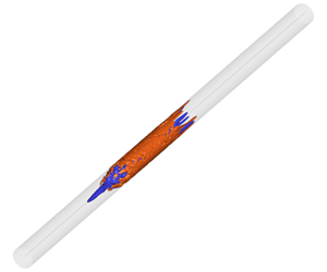
Evolution of the rescaled nonlinear optimal solution at  $Ma=0.50$. Isosurfaces of
 $u_{1}^{\prime }=0.60\times \max (u_{1}^{\prime })$ (red) and
 $u_{1}^{\prime }=-0.60\times \max (u_{1}^{\prime })$ (blue) at
 $t=35$.

The results presented so far have shown the energy amplification of nonlinear disturbances in orderly laminar flow. To investigate the potential of the nonlinear optimal perturbations to trigger a chaotic state, we increase the initial kinetic energy by multiplying the optimal initial condition computed for the case  $Ma=0.50$ by a factor of 5.3, so that
 $E_{0}/Ma^{2}=2.0\times 10^{-6}$. The rescaled perturbation field is used as an initial condition and advanced over an increased horizon of 71 time units. The resulting evolution of the perturbation kinetic energy is presented in figure 9. The perturbations initially amplify via the Orr and lift-up mechanisms before the emergence of a chaotic state at
 $t\approx 26$ further enhances the energy level. Eventually, the convection of the perturbation field out of the computational domain gradually decreases the integral perturbation kinetic energy level. A visualization of the perturbation field at
 $t=35$ is presented in figure 10 and shows that the pattern of streaks has begun to develop into a broadband chaotic state which should, however, not be confused with developed turbulence. We also note that this type of analysis is not a substitute for the identification of an actual minimal seed which may induce turbulence at lower kinetic energy and at an earlier time.
Lastly, we compare the evolution of nonlinear optimal perturbations at high kinetic energy at different Mach numbers. For this purpose, we iteratively rescale the initial energy level of the optimal perturbations computed for the various Mach numbers so as to attain the same kinetic energy of  $E(t)/Ma^{2}=0.016$ at time
 $t=22$. This energy level matches that observed in figure 9 at the onset of the chaotic regime, at
 $t\approx 26$. The identified scaling factors by which the initial energy is modified are
 $A=8.90$,
 $6.80$,
 $2.50$ and
 $1.90$ for the cases
 $Ma=0.20$,
 $0.50$,
 $0.65$ and
 $0.80$, respectively. As evidenced in figure 11(a), the level of kinetic energy required to reach the target value thus decreases with Mach number, demonstrating that the cases at higher Mach number require lower initial kinetic energy to reach the same kinetic energy at final time. Consistent with this result, the evolution of the normalized energy,
 $E(t)/E_{0}$, presented in figure 11(b), substantiates a strong increase of the associated growth with Mach number.
Time evolution of kinetic energy for high-energy perturbations. (a) Kinetic energy normalized by the square of the Mach number,  $E(t)/Ma^{2}$. (b) Kinetic energy normalized by the initial perturbation kinetic energy,
 $E(t)/E_{0}$.
 $Ma=0.20$ (black),
 $Ma=0.50$ (red),
 $Ma=0.65$ (purple) and
 $Ma=0.80$ (blue).

4 Conclusions
A variational framework for the identification of general nonlinear optimal perturbations in compressible flows has been presented. The formulation is based on the compressible Navier–Stokes equations in conserved variables for an ideal gas with temperature-dependent viscosity. The implemented method was validated in the limit of low Mach numbers against published data on incompressible, effectively periodic pipe flow. Both the linear and nonlinear optimal perturbations are captured and the transient energy gain were shown to match results reported by Pringle & Kerswell (Reference Pringle and Kerswell2010). At higher Mach numbers, the pipe flow becomes increasingly non-periodic. The associated nonlinear optimal perturbations are spatially localized and their growth describes a sequence of Orr mechanism, oblique nonlinear interaction and lift-up mechanism. Qualitatively, the amplification of the perturbations is thus similar to incompressible periodic pipe flow (Pringle et al. Reference Pringle, Willis and Kerswell2012), although the observed amplification in kinetic energy is appreciably higher than in the incompressible regime. Nonlinear optimal disturbances which have been rescaled to a higher initial kinetic energy than prescribed in the optimization procedure were shown to eventually reach a chaotic state. It was further shown that for a constant time horizon, the initial perturbation energy to reach a prechaotic high-energy state decreases monotonically with Mach number.
Acknowledgements
The authors wish to thank T. Flint for many helpful discussions. This research was supported by the Office of Naval Research under grant N00014-17-1-2341.
Declaration of interests
The authors report no conflict of interest.



