Nomenclature
-
 $b$
-
thrust factor
-
$d$
-
drag factor
-
$g$
-
gravitational acceleration
-
$m$
-
quadcopter mass
-
$\boldsymbol{r}$
-
position vector in NED frame
-
${u_F}$
-
total thrust force
-
${\boldsymbol{u}_\tau }$
-
torque control vector
-
$x,y,z$
-
position in NED frame
- CoG
-
centre of gravity
-
${F_i}$
-
thrust force of individual rotor
-
$L$
-
distance from the propeller to CoG
-
${I_r}$
-
motor moment of inertia
-
${I_{xx}},{I_{yy}},{I_{zz}}$
-
inertias around
$x,y,z$
axes -
${K_{{p_{\mathrm{*}}}}},{K_{{i_{\mathrm{*}}}}},{K_{{d_{\mathrm{*}}}}}$
-
proportional, integral and derivative gains
-
$\boldsymbol{R}$
-
rotation matrix


Greek symbol
-
$\phi $
-
roll angle
-
$\theta $
-
pitch angle
-
$\boldsymbol\xi $
-
orientation vector
-
$\psi $
-
yaw angle
-
${{\mathrm{\Omega }}_i}$
-
angular speed of each motor


1.0 Introduction
Unmanned air vehicles (UAVs) can be operated autonomously or remotely via a flight control system. Unlike manned aircraft, UAVs do not risk pilot lives during operation. Advanced technological developments have enhanced UAV manoeuverability, reduced manufacturing costs, and simplified assembly processes. Due to these advantages, UAVs have gained widespread popularity in the aviation industry and are increasingly used for hobby purposes.
Quadcopters, a type of UAV with rotary wings, have attracted significant attention from researchers over the past two decades. Often referred to as drones in military contexts, quadcopters have become a prominent research topic due to features such as vertical take-off and landing capabilities, light weight and extended endurance [Reference Mardan, Esfandiari and Sepehri1,Reference Saif and Eminoğglu2]. These advantages make quadcopters widely used in military operations, search-and-rescue missions, agriculture, mapping, surveillance and reconnaissance [Reference Zainuddin, Ghazali and Mat Arof3–Reference Ju, Kim, Seol and Il Son5]. However, the attitude control of quadcopters presents ongoing challenges due to aerodynamic uncertainties, the nonlinear nature of their dynamics, parameter uncertainties and sensitivity to environmental factors [Reference Mian and Daobo6–Reference Kamal Hosseini Sani and Kakavand8]. Thus, an effective controller is essential for overcoming these challenges and achieving successful trajectory tracking missions [Reference Zhu, Cabecinhas, Xie, Casau, Silvestre, Batista and Oliveira9].
In recent years, more complex controllers have been tested for altitude and attitude control of quadcopters. Advanced control methods often draw inspiration from traditional ones found in the literature. PID, LQR, and H-infinity are well-known examples of linear control methods [Reference Ataka, Tnunay, Inovan, Abdurrohman, Preastianto, Cahyadi and Yamamoto10–Reference Alexandrov, Rezkov, Shatov and Chestnov12]. Nonlinear control methods such as feedback linearisation, model predictive control, backstepping control, sliding mode control and adaptive control [Reference Bhatia, Jiang, Zhen, Ahmed and Rohra13–Reference Farber and Richards17], are developed to address the stability and robustness of systems affected by external disturbances and uncertainties [Reference Roy, Islam, Sadman, Mahmud, Gupta and Ahsan18]. Additionally, fuzzy methods and artificial neural networks have become popular for model-free, learning-based controllers in recent years [Reference Jiang, Pourpanah and Hao19–Reference Guzay and Kumbasar21].
Although various approaches have been tested and implemented for UAV control under a wide range of flight conditions, the PID controller still holds a significant place in flight control systems. PID controllers are favoured in industrial applications for their easy implementation, straightforward design process, ability to reduce steady-state error through parameter tuning and low computational demand [Reference Jiao, Liu, Zhang and Lian22–Reference Idrissi, Salami and Annaz24]. However, classical PID tuning methods may not always yield satisfactory results in precision control applications, prompting the use of artificial intelligence-based algorithms for fine-tuning PID gains in recent years [Reference Wang, Lee, Fung, Bi and Zhang25].
Traditional approaches such as the Ziegler-Nichols [Reference Ziegler and Nichols26] and Cohen-Coon [Reference Cohen and Coon27] methods have been used to tune PID gains. Recent studies have evaluated various tuning techniques; for instance, proportional-derivative (PD) controllers tuned using adaptive particle swarm optimisation (APSO) and Ziegler-Nichols (ZN) methods were tested on a quadcopter, revealing that APSO-based PD controllers delivered superior tracking accuracy, shorter settling times, and lower overshoots compared to those tuned with ZN methods [Reference Yazid, Garrat and Santoso28]. However, this study only focused on tuning parameters for position control and did not consider fine-tuning attitude controllers for safety reasons.
Another study developed a comprehensive model of a quadcopter, incorporating gyroscopic moments, external disturbances such as wind and the Earth’s atmospheric rotation. This complex model was used to design individual PID controllers for each translational and rotational motion in all three axes [Reference Parfiryev, Ischuk, Dushkin and Smolyakova29]. Unlike the previous study, the ZN method was utilised to tune PID coefficients. Further research compared the Ziegler-Nichols-based PID and the self-tuning fuzzy PID controllers on a linear quadcopter model to achieve fine-tuning of the attitude and altitude controllers. It was concluded that the self-tuning fuzzy PID controller improved time response characteristics in terms of settling time and overshoot [Reference Sarbass, Tatli and Onrat30]. Another ZN-based PID controller was also introduced for attitude control of an X-configuration quadcopter without considering the position control. It was assumed that applying the ZN-based optimisation procedure only for tuning PID coefficients for pitch movement was sufficient due to the symmetric structure of the quadcopter. The results indicated that although the ZN-based PID controller produced lower rise times in the pitch axis, the PSO-based PID controller provided better overall control performance [Reference Khodja, Tadjine, Boucherit and Benzaoui31]. However, traditional PID tuning methods cannot produce satisfactory responses in precise control applications, which is why AI-based algorithms have been increasingly used in recent years to tune PID coefficients.
In a relevant study, a PD controller was implemented into two distinct control architectures for both altitude and attitude control of a quadcopter in hover flight mode [Reference Artale, Milazzo, Orlando and Ricciardello32]. The first architecture utilised a genetic algorithm (GA) and particle swarm optimisation (PSO) to design PD controllers for a nonlinear quadcopter model, while the second used an LQR-based PD controller for a linear model. In the latter case, PSO and GA first optimised the weighting matrices of the LQR controller, which was then used to tune PD gains. The simulation results indicated that the PSO-based PD controller provided the best performance for ISE and their own performance index, while the GA-based PD excelled in IAE values. In another study, a robust controller was developed to manage weight variations in quadcopters, employing both PSO-based PID and differential evaluation (DE)-based PID controllers [Reference Can and Ercan33]. These controllers were designed to enable the quadcopter to follow a straight trajectory along the x-axis and maintain its initial position in the y-z plane. Tested in the GAZEBO simulation environment across different quadcopter weights, the evolutionary optimisation algorithms outperformed classical tuning methods in terms of controller effectiveness.
The gains of four individual PID controllers were separately tuned using GA, evolution strategies (ES), DE, and cuckoo search (CS) algorithms for a linear quadcopter model controlling motions in the x-y plane, z-axis and roll-pitch-yaw axes. To assess these methods, two different flight trajectories were established. The results varied per trajectory and controller, with GA and ES generally outperforming the others [Reference Hasseni, Abdou and Glida34]. The PSO method was also compared with the GA method for tuning classical PID and fractional order PID (FOPID) controllers using a linear quadcopter model. The findings showed that PSO-FOPID delivered superior performance in the x-y, z, roll-pitch axes, while the PSO-PID controller was more effective in the yaw axis [Reference Saribas and Kahvecioglu35]. These studies predominantly used a linear model for tuning PID coefficients, focusing mainly on attitude stabilisation, which can compromise control performance during tracking flight missions. Therefore, there is a need for a more efficient optimisation procedure to tune PID coefficients for successful tracking in autonomous flight missions. Since nature-inspired optimisation algorithms require a mathematical model of the controlled system, this study proposes an alternative optimisation procedure with a modified multi-objective function based on a nonlinear quadcopter model. Moreover, the PID coefficients used in the attitude and position controllers are simultaneously tuned during the optimisation process for a trajectory path designed in 3D space.
In this study, a cascade PID control algorithm is designed using a nonlinear model of a quadcopter. Three PID controllers are used in the inner loop and three in the outer loop. The outer loop controls the position of the quadcopter, aiming to move it to desired locations and regulate the attitude angles—roll, pitch and yaw—along with the required total thrust force. The desired attitude angles are then sent to the inner loop, where the attitude controller generates the necessary torques around the roll, pitch and yaw axes. The fine-tuning of controller gains has been adjusted with PSO, grey wolf optimisation (GWO), artificial bee colony (ABC), and (DE). Integral time absolute error (ITAE), integral time square error (ITSE), integral square error (ISE), and integral absolute error (IAE) criteria are selected as the fitness functions for the optimisation algorithms. A modified multi-objective function was designed by weighting the position and attitude errors in these fitness functions according to their effects on the system responses. The tracking performance of the designed controller has been tested in simulations. Square and spiral trajectories were generated, and the results of the simulation studies showed that the algorithms used to optimise the PID coefficients provide successful results. Additionally, the controller performances under bounded disturbances were analysed. The robustness analysis, considering important effects such as ground effect, wind effect and mass variation, was performed using the fine-tuned PID gains from previous simulations.
2.0 Modeling of quadcopter
A generic quadcopter consists of four separate rotors, each mounted on a symmetric framework, with each rotor connected by an identical link. Each rotor is operated by an electrical motor. Generally, two of them rotate in a clockwise direction, while the others rotate in a counter-clockwise direction. This arrangement guarantees zero net torque around the vertical axis at the CoG (centre of gravity) point, as shown in Fig. 1.
The configuration of quadcopter UAV with respect to its frames.

In the derivation of the quadcopter model, some generally accepted assumptions are made: i) the quadcopter possesses a rigid and symmetric structure, and ii) the origin
 ${O_b}$
of the body-fixed frame
 ${\mathcal{F}_B}$
coincides with the CoG. To represent the dynamics of the translational and rotational motions of the quadcopter by using Newton-Euler formulation, a North-East-Down (NED) inertial frame
 ${\mathcal{F}_E}$
, attached to the Earth, and a body-fixed frame
 ${\mathcal{F}_B}$
are defined. The position of the quadcopter is given by the vector
 $r = {\left[ {x,y,z} \right]^{\rm T}}$
in the frame
 ${\mathcal{F}_E}$
and the orientation of the quadcopter is defined by the vector
 $\xi = {\left[ {\phi, \theta, \psi } \right]^{\rm T}}$
, which includes Euler angles (i.e. roll, pitch and yaw, respectively) in the frame
 ${\mathcal{F}_B}$
with respect to the frame
 ${\mathcal{F}_E}$
. The translational dynamics of the quadcopter in three-dimensional space
 ${\mathbb{R}^3}$
are given as:
 \begin{align}\ddot r = g\nu - \frac{1}{m}R{u_F}\end{align}
where the unit vector
 $\upsilon = {[\begin{array}{*{20}{l}}0\;\; {}0\;\; {}1\end{array}\!]^{\rm T}}$
and the transformation matrix
 $R$
from the body-fixed to the inertial reference frame system is given by
 \begin{align*}R = \left[ {\begin{array}{*{20}{l}}{{{\mathrm{c}}_\psi }{{\mathrm{c}}_\theta }}\quad {}{{{\mathrm{c}}_\psi }{{\mathrm{s}}_\theta }{{\mathrm{s}}_\phi } - {{\mathrm{s}}_\psi }{{\mathrm{c}}_\phi }}\quad {{{\mathrm{c}}_\psi }{{\mathrm{s}}_\theta }{{\mathrm{c}}_\phi } + {{\mathrm{s}}_\psi }{{\mathrm{s}}_\phi }}\\{{{\mathrm{s}}_\psi }{{\mathrm{c}}_\theta }}\quad {}{{{\mathrm{s}}_\psi }{{\mathrm{s}}_\theta }{{\mathrm{s}}_\phi } + {c_\psi }{{\mathrm{c}}_\phi }}\quad {{{\mathrm{s}}_\psi }{{\mathrm{s}}_\theta }{{\mathrm{c}}_\phi } - {{\mathrm{c}}_\psi }{{\mathrm{s}}_\phi }}\\{ - {{\mathrm{s}}_\theta }}\quad {{{\mathrm{c}}_\theta }{{\mathrm{s}}_\phi }}\quad\quad\quad\quad\quad {{{\mathrm{c}}_\theta }{{\mathrm{c}}_\phi }}\end{array}} \right]\end{align*}
where
 ${{\mathrm{c}}_{\mathrm{*}}} = {\mathrm{cos}}\left( {\mathrm{*}} \right)$
and
 ${{\mathrm{s}}_{\mathrm{*}}} = {\mathrm{sin}}\left( {\mathrm{*}} \right)$
. The total thrust force,
 ${u_F}$
, is the sum of the individual thrusts,
 ${F_i}$
, produced by each rotor driven by an electrical motor, expressed as
 ${u_F} = \mathop \sum \nolimits_{i = 1}^4 {F_i}$
with
 ${F_i} = b{{\mathrm{\Omega }}_i}$
where
 $b$
is the thrust factor and
 ${{\mathrm{\Omega }}_i}$
is the angular speed of each motor.
The rotational dynamics of the quadcopter are expressed as follows:
 \begin{align}\boldsymbol{I}\boldsymbol{\ddot \xi} = - \boldsymbol{\dot \xi} \times \boldsymbol{I}\boldsymbol{\dot \xi} - \boldsymbol{I}_{\boldsymbol{r}}\boldsymbol{\dot \xi} \times \boldsymbol{\Omega} + \boldsymbol{u}_{\boldsymbol{\tau}}\end{align}
where
 $\boldsymbol{\Omega} = \left[ {\begin{array}{*{20}{l}}0\;\; {}0\;\; {}{{{\mathrm{\Omega }}_r}}\end{array}} \!\right]$
with
 ${{\mathrm{\Omega }}_r} = {{\mathrm{\Omega }}_1} - {{\mathrm{\Omega }}_2} + {{\mathrm{\Omega }}_3} - {{\mathrm{\Omega }}_4}$
,
 ${I_r}$
represents the rotor moment of inertia,
 $\boldsymbol{I} = {\mathrm{diag}}\left( {{I_{xx}},{I_{yy}},{I_{zz}}} \right)$
denotes the moments of inertia with respect to its principal axes, and
 $\boldsymbol{u}_{\boldsymbol{\tau}} = {\left[ {\begin{array}{*{20}{l}}{{u_\phi }}\;\; {}{{u_\theta }}\;\; {}{{u_\psi }}\end{array}} \!\right]^{\rm T}}$
is the torque control vector. The complete dynamic model of the quadcopter can now be assembled as follows:
 \begin{align*}{I_{xx}}\ddot \phi &= \left( {{I_{yy}} - {I_{zz}}} \right)\dot \theta \dot \psi - {I_r}\dot \theta {{\mathrm{\Omega }}_r} + {u_\phi }\\{I_{yy}}\ddot \theta &= \left( {{I_{zz}} - {I_{xx}}} \right)\dot \phi \dot \psi + {I_r}\dot \phi {{\mathrm{\Omega }}_r} + {u_\theta }\\{I_{zz}}\ddot \psi &= \left( {{I_{xx}} - {I_{yy}}} \right)\dot \theta \dot \phi + {u_\psi }\\m\ddot x &= - \left( {{{\mathrm{c}}_\psi }{{\mathrm{s}}_\theta }{{\mathrm{c}}_\phi } + {{\mathrm{s}}_\psi }{{\mathrm{s}}_\phi }} \right){u_F}\\m\ddot y &= - \left( {{{\mathrm{s}}_\psi }{{\mathrm{s}}_\theta }{{\mathrm{c}}_\phi } - {{\mathrm{c}}_\psi }{{\mathrm{s}}_\phi }} \right){u_F}\\m\ddot z &= mg - \left( {{{\mathrm{c}}_\theta }{{\mathrm{c}}_\phi }} \right){u_F}\end{align*}
where the control inputs are defined as
 \begin{align}\left[ {\begin{array}{*{20}{l}}{{u_\phi }}\\{{u_\theta }}\\{{u_\psi }}\\{{u_F}}\end{array}} \right] = \left[ {\begin{array}{c@{\quad}c@{\quad}c@{\quad}c}0 & {Lb} {}& 0 {}& {-Lb}\\ {Lb} & 0 & {-Lb} & 0\\ d & {-d} & d & {-d}\\b & b & b & b\end{array}} \right]\left[ {\begin{array}{*{20}{l}}{{\mathrm{\Omega }}_1^2}\\[2pt]{{\mathrm{\Omega }}_2^2}\\[2pt]{{\mathrm{\Omega }}_3^2}\\[2pt]{{\mathrm{\Omega }}_4^2}\end{array}} \right]\end{align}
where
 $L$
is the distance from the propeller to the CoG and
 $d$
is the drag factor. The model parameters of the quadcopter used as an example are given in Table 1 [Reference Kayacan and Maslim36].
Quadcopter parameters

3.0 Design of the cascade pid controller
The classical control architecture typically includes only a single feedback loop. This structure often suffers from poor robustness performance when disturbances affect the plant under control, potentially resulting in slow settling times or high steady-state errors. To mitigate these disadvantages, a cascade control architecture can be employed, as depicted in Fig. 2.
A general cascade control architecture.

This structure yields higher effectiveness in terms of control measures, particularly when the inner loop operates faster than the outer loop and when disturbances applied to the inner loop are effectively suppressed, thus mitigating the impact on the plant [Reference Oh, Jang and Pedrycz37–Reference Soares, Calil and Stephan39]. Generally, this control structure comprises two interlinked feedback loops: the inner and outer loops. The outer loop generates the command input for the inner loop, serving as the set-point.
In the control architecture developed here, the inner loop is tasked with performing attitude control, while the outer loop is designed to manage the altitude and the motion in the
 $x - y$
plane of the quadcopter. The outer loop generates the desired roll and pitch angles, denoted
 ${\phi _d}$
and
 ${\theta _d}$
, respectively. The yaw angle
 $\psi $
is maintained at zero throughout the flight, except when another PID controller, tuned via an optimisation method, is implemented to track a desired non-zero yaw angle. As depicted in Fig. 2,
 $\boldsymbol{r}_\boldsymbol{d} = {\left[ {{x_d},{y_d},{z_d}} \right]^{\rm T}}$
represents the desired positions defined in the frame
 ${\mathcal{F}_E}$
, and the position error vector for the outer loop is given by
 ${[{e_x},{e_y},{e_z}]^{\mathrm{{\rm T}}}}$
calculated as
 ${[{x_d} - x,{y_d} - y,{z_d} - z]^{\mathrm{{\rm T}}}}$
. The position control of the quadcopter in the outer loop is executed using individual PID controllers for each axis, with the corresponding control inputs specified below:
 \begin{align}{{u_x}} {}{ = {K_{{p_x}}}{e_x} + {K_{{i_x}}}\mathop \int \nolimits_0^t {e_x}dt + {K_{{d_x}}}{{\dot e}_x}}\nonumber\\{{u_y}} {}{ = {K_{{p_y}}}{e_y} + {K_{{i_y}}}\mathop \int \nolimits_0^t {e_y}dt + {K_{{d_y}}}{{\dot e}_y}}\\{{u_z}} {}{ = {K_{{p_z}}}{e_z} + {K_{{i_z}}}\mathop \int \nolimits_0^t {e_z}dt + {K_{{d_z}}}{{\dot e}_z}}\nonumber\end{align}
where
 ${K_{{p_{\mathrm{*}}}}}$
,
 ${K_{{i_{\mathrm{*}}}}}$
and
 ${K_{{d_{\mathrm{*}}}}}$
are, respectively, the proportional, integral and derivative gains. Here, the subscript * indicates the corresponding axis (
 $x$
,
 $y$
or
 $z$
axis). The control inputs (4) are utilised to determine the desired attitude angles and the total thrust force as follows:
 \begin{align}{u_F} = m\sqrt {u_x^2 + u_y^2 + {{({u_z} + g)}^2}} \end{align}
 \begin{align}{\phi _d} = {\mathrm{arcsin}}\left( { - \frac{{{u_y}}}{{\sqrt {u_x^2 + u_y^2 + {{({u_z} + g)}^2}} }}} \right)\end{align}
 \begin{align}{\theta _d} = {\mathrm{arctan}}\left( {\frac{{{u_x}}}{{{u_z} + g}}} \right)\end{align}
In order to maintain the desired attitudes, a PID controller is separately designed for yaw, roll and pitch axes, similar to the method used for controlling the position of the quadcopter. Therefore, the torque control inputs can be computed as follows:
 \begin{align}{{u_\phi }} & { = {K_{{p_\phi }}}{e_\phi } + {K_{{i_\phi }}}\mathop \int \nolimits_0^t {e_\phi }dt + {K_{{d_\phi }}}{{\dot e}_\phi }}\nonumber\\{{u_\theta }} & { = {K_{{p_\theta }}}{e_\theta } + {K_{{i_\theta }}}\mathop \int \nolimits_0^t {e_\theta }dt + {K_{{d_\theta }}}{{\dot e}_\theta }}\\{{u_\psi }} & { = {K_{{p_\psi }}}{e_\psi } + {K_{{i_\psi }}}\mathop \int \nolimits_0^t {e_\psi }dt + {K_{{d_\psi }}}{{\dot e}_\psi }}\nonumber\end{align}
where
 ${e_\phi }$
,
 ${e_\theta }$
and
 ${e_\psi }$
denote the attitude errors, i.e.
 ${e_\phi } = {\phi _d} - \phi $
,
 ${e_\theta } = {\theta _d} - \theta $
and
 ${e_\psi } = {\psi _d} - \psi $
. Here,
 ${K_{{p_{\mathrm{*}}}}}$
,
 ${K_{{i_{\mathrm{*}}}}}$
and
 ${K_{{d_{\mathrm{*}}}}}$
are the proportional, integral and derivative gains, respectively. The subscript * indicates the corresponding axis (
 $\phi $
,
 $\theta $
or
 $\psi $
). Now, the motor speeds required to track the desired positions and attitudes can be calculated by taking the inverse of (3), given by:
 \begin{align*}\left[ {\begin{array}{*{20}{l}}{{\mathrm{\Omega }}_1^2}\\[2pt]{{\mathrm{\Omega }}_2^2}\\[3pt]{{\mathrm{\Omega }}_3^2}\\[3pt]{{\mathrm{\Omega }}_4^2}\end{array}} \right] = \left[ {\begin{array}{*{20}{l}}{\frac{1}{{4b}}{u_F} + \frac{1}{{4d}}{u_\psi } + \frac{1}{{2Lb}}{u_\theta }}\\[3pt]{\frac{1}{{4b}}{u_F} - \frac{1}{{4d}}{u_\psi } + \frac{1}{{2Lb}}{u_\phi }}\\[3pt]{\frac{1}{{4b}}{u_F} + \frac{1}{{4d}}{u_\psi } - \frac{1}{{2Lb}}{u_\theta }}\\[3pt]{\frac{1}{{4b}}{u_F} - \frac{1}{{4d}}{u_\psi } - \frac{1}{{2Lb}}{u_\phi }}\end{array}} \right]\end{align*}
4.0 Optimisation algorithms
In this section, the optimisation algorithms employed to fine-tune the PID gains, as specified in (4) and (8), are briefly introduced. Figure 3 illustrates the generic optimisation procedure utilised in the simulations.
The flowchart used in the optimisation mechanism.

4.1 Particle swarm optimsation
Particle swarm optimisation (PSO) is a population-based optimisation method, first developed by Kennedy and Eberhart in 1995 [Reference Eberhart and Kennedy40]. They drew inspiration from the social behaviours observed in schools of fish and flocks of birds.
PSO has gained popularity as an optimisation technique due to its minimal control parameter requirements and straightforward structure. In PSO, the current position of each individual in a swarm is recorded. This includes the position of the individual with the best value in the current iteration (
 ${P_{best}}$
) and the position with the best global value (
 ${G_{best}}$
).
 ${P_{best}}$
converges towards
 ${G_{best}}$
as each individual shares its location with others throughout the optimisation process [Reference Shi and Eberhart41]. The velocity of each individual is then computed and their positions are updated using:
 \begin{align}v_{ij}^{k + 1} &= wv_{ij}^k + {c_1}{r_1}\left( {{\mathrm{pbest}}_{ij}^k - x_{ij}^k} \right) + {c_2}{r_2}\left( {{\mathrm{gbest}}_{ij}^k - x_{ij}^k} \right)\end{align}
 \begin{align}x_{ij}^{k + 1} &= x_{ij}^k + v_{ij}^{k + 1}\end{align}
where
 ${c_1}$
and
 ${c_2}$
are acceleration constants that regulate each individual’s convergence rate to its best position. High acceleration constants can cause individuals to overshoot their best positions, while low values might prevent reaching these positions altogether.
 ${r_1}$
and
 ${r_2}$
are random numbers between 0 and 1. The inertia weight
 $w$
is also chosen from a range of 0 to 1; higher values facilitate global search capabilities, while lower values enhance local search effectiveness.
 ${\mathrm{pbest}}_{ij}^k$
is the best solution reached by the individual
 $i$
up to iteration
 $k$
, and
 ${\mathrm{gbest}}_{ij}^k$
is the best solution found in the group up to iteration
 $k$
.
 $v_{ij}^k$
and
 $x_{ij}^k$
denote the velocity and position of individual
 $i$
at iteration
 $k$
, respectively. After updates, the fitness values of all individuals in the new population are recomputed, and these computations are repeated until the maximum allowed number of iterations is reached.
4.2 Differential evolution (DE)
Differential evolution (DE), first introduced in 1995 by Rainer Storn and Kenneth Price, is based on a population-based optimisation algorithm. DE is a meta-heuristic algorithm that simulates natural evolution by combining different individuals to generate new ones with superior fitness values [Reference Storn and Price42].
The DE algorithm employs three distinct operators: mutation, crossover and selection. To produce a new individual, DE uses a differential mutation operator that combines three randomly selected individuals from the current population. A new candidate solution is then generated by combining this mutation with the current individual using a crossover operator. The selection of the individual subject to mutation and the transition point is stochastic, enabling the algorithm to explore the search space randomly. The new population is evaluated using an objective function, and the best solutions are stored for the next iteration [Reference Storn and Price42].
The initial population is generated by
 \begin{align*}{X_{i,j}} = {X_{min}} + {\mathrm{rand}}\left[ {0,1} \right]\left( {{X_{max}} - {X_{min}}} \right)\end{align*}
where
 ${X_{i,j}}$
represents the candidate solution, and
 ${X_{min}}$
and
 ${X_{max}}$
denote the lower limit and upper limit. Here,
 ${\mathrm{rand}}\left[ {0,1} \right]$
is a random number between 0 and 1. In the mutation process, new solutions are are formulated as:
 \begin{align*}{Y_i} = {X_{r1}} + F\left( {{X_{r2}} - {X_{r3}}} \right)\end{align*}
where
 ${Y_i}$
is the new solution and
 ${X_{r1}}$
,
 ${X_{r2}}$
and
 ${X_{r3}}$
are the three randomly selected solutions.
 $F$
is a scale factor, typically set between 0 and 2. The crossover process is then performed as follows:
 \begin{align*} {Z_i} = \begin{cases}{{Y_{i,j}}} & {}{{\mathrm{rand}}\left[ {0,1} \right] \lt CR}\\ {{X_{i,j}}} & {}{{\mathrm{otherwise}}} \end{cases} \end{align*}
where
 $CR$
is the crossover ratio. Finally, in the selection stage, the choice is made based on the following criterion:
 \begin{align*} {X_{i,j}} = \begin{cases}{{Z_i}} & {f\left( {{Z_i}} \right) \le f\left( {{X_{i,j}}} \right)}\\{{X_{i,j}}} & {{\mathrm{otherwise}}}\end{cases} \end{align*}
4.3 Artificial bee colony (ABC)
First proposed in 2005 by Dervis Karaboga, inspired by the food search behaviour of honey bees [Reference Karaboga43], the ABC algorithm is a swarm intelligence-based optimisation method. It consists of three different bee populations: employed bees, onlooker bees and scout bees. Employed bees are tasked with searching for better solutions near the current solution. When a new solution is discovered, it is compared with the current solution; if superior, the current solution is updated; otherwise, it is retained. Subsequently, employed bees share their solutions with onlooker bees, who then search for the best solution among those provided by the employed bees. Scout bees are tasked with exploring new regions within the search space to discover superior solutions. When a food source is exhausted, the corresponding employed bee transitions into a scout bee.
The locations of the initial food sources are determined by:
 \begin{align}{x_{ij}} = x_j^{min} + {\mathrm{rand}}\left[ {0,1} \right]\!\left( {x_j^{max} - x_j^{min}} \right)\end{align}
with
 $i = 1,2, \ldots, $
N and
 $j = 1,2, \ldots, M$
where
 $M$
and
 $N$
denote the number of the food sources and the parameters to be optimised, respectively. A new source is then generated for the employed bee associated with the solution
 ${x_i}$
using:
 \begin{align}{v_{ij}} = {x_{ij}} + {{\mathrm{\Phi }}_{ij}}\!\left( {{x_{ij}} - {x_{kj}}} \right)\end{align}
subject to
 \begin{align*}{v_{ij}} = \left\{ {\begin{array}{*{20}{l}}{x_j^{min}} {}{{v_{ij}} \lt x_j^{min}}\\{{v_{ij}}} {}{x_j^{min} \le {v_{ij}} \le }\\{x_j^{max}} {}{{v_{ij}} \gt x_j^{max}}\end{array}} \right.x_j^{max}\end{align*}
where
 ${v_{ij}}$
is a candidate solution and
 ${{\mathrm{\Phi }}_{ij}} \in \left[ { - 1,1} \right]$
is a random number. The probability value
 ${P_i}$
used by the onlooker bees in the selection process is calculated by
 \begin{align*}{P_i} = \frac{{{\mathrm{fi}}{{\mathrm{t}}_i}}}{{\mathop \sum \nolimits_{i = 1}^N {\mathrm{fi}}{{\mathrm{t}}_i}}}\end{align*}
In the roulette wheel selection mechanism, a random number between 0 and 1 is generated for each source. If the random number is less than
 ${P_i}$
, then a new source is generated using (12). If the new source is superior to the current source, it replaces the current source and the dimension failure is reset. Otherwise, the dimension failure count is incremented by one. This process is repeated until all onlooker bees have settled into food source areas. Dimension failures are then reviewed, and a new source is generated using (11) for the exhausted sources. Subsequently, the best solution is recorded. Finally, all these steps are repeated until the stopping criterion is met.
4.4 Grey wolf optimisation (GWO)
The grey wolf optimiser (GWO) is a swarm intelligence-based metaheuristic algorithm first proposed by Mirjalili et al. in 2014 [Reference Mirjalili, Mirjalili and Lewis44]. The GWO algorithm is inspired by the hunting behaviour, leadership and social hierarchy observed in grey wolf packs, which include four distinct ranks: alpha (
 $\alpha $
), beta (
 $\beta $
), delta (
 $\delta $
) and omega (
 $\omega $
). This algorithm models the wolves’ tactics of encircling, hunting and attacking their prey. In the wild, grey wolves encircle their prey and coordinate their attacks, a strategy that is emulated in GWO by dividing the search space into subspaces assigned to each wolf.
The encircling behaviour is mathematically modeled by:
 \begin{align*}\vec D = \left| {\vec C{{\vec X}_p}(t) - \vec X(t)} \right|\end{align*}
 \begin{align*}\vec X\left( {t + 1} \right) = {\vec X_p}(t) - \vec A \cdot \vec D\end{align*}
where
 $t$
denotes the iteration step,
 $\vec A$
and
 $\vec C$
are the coefficient vectors,
 ${\vec X_p}$
denotes the position of the prey, and
 $\vec X$
is the position vector of a grey wolf. The coefficients
 $\vec A$
and
 $\vec C$
are calculated as follows:
 \begin{align*}\vec A &= 2\vec a \cdot {\vec r_1} - \vec a \\\vec C &= 2{\vec r_2}\end{align*}
where components of
 $\vec a$
linearly decrease from 2 to 0 across each iteration, and
 ${\vec r_1}$
and
 ${\vec r_2}$
are random vectors within the range of 0 to 1. The hunting behaviour is mathematically represented by:
 \begin{align*}{\vec D_\alpha } = \left| {{{\vec C}_1}{{\vec X}_\alpha } - \vec X} \right|\\{\vec D_\beta } = \left| {{{\vec C}_2}{{\vec X}_\beta } - \vec X} \right|\\{\vec D_\delta } = \left| {{{\vec C}_3}{{\vec X}_\delta } - \vec X} \right|\end{align*}
and
 \begin{align*}{\vec X_1} &= {\vec X_\alpha } - {\vec A_1} \cdot {\vec D_\alpha }\\{\vec X_2} &= {\vec X_\beta } - {\vec A_2} \cdot {\vec D_\beta }\\{\vec X_3} &= {\vec X_\delta } - {\vec A_3} \cdot {\vec D_\delta }\\\vec X\left( {t + 1} \right) &= \frac{{{{\vec X}_1} + {{\vec X}_2} + {{\vec X}_3}}}{3}\end{align*}
where the subscripts
 $\alpha $
,
 $\beta $
and
 $\delta $
denote the wolves in the wolf pack. The attacking phase is initiated when
 $\left| {\vec A} \right| \geqslant 1$
, allowing the pack to search the area, and approaches the prey (or optimum solution) when
 $\left| {\vec A} \right| \lt 1$
.
5.0 Fitness function
The PID controller aims to eliminate the error between the desired and current trajectories. However, completely eradicating this tracking error in real-time applications is not feasible. Instead, control practitioners strive to minimise the error as much as possible.
The control architecture proposed in this study incorporates six distinct PID controllers, as detailed in Section 3.0. The PSO algorithm is employed to minimise both the tracking errors and the optimisation time. Consequently, the most critical step involves designing an appropriate fitness function. The fitness functions used for the optimisation process are based on well-known performance measures, including IAE, ISE, ITSE, and ITAE. These fitness functions are defined as follows:
 \begin{align}{J_i} = \left\{ {\begin{array}{*{20}{l}}{\smallint {e_i}{{(t)}^2}dt,} & {{\mathrm{for\;ISE}}}\\{\smallint \left| {{e_i}(t)} \right|dt,} & {{\mathrm{for\;IAE}}}\\{\smallint t\left| {{e_i}(t)} \right|dt,} & {{\mathrm{for\;ITAE}}}\\{\smallint t\left[ {{e_i}{{(t)}^2}} \right]dt,} & {{\mathrm{for\;ITSE}}}\end{array}} \right.\end{align}
where
 ${e_i}(t)$
denotes the tracking error in the corresponding state. Utilising the fitness function (13), the objective function is expressed as:
 \begin{align*}J = \mathop \sum \limits_{i = 1}^n {\tilde J_i}\end{align*}
where
 $n$
is the dimension of the state vector and
 ${\tilde J_i}$
is the weighted fitness function defined by
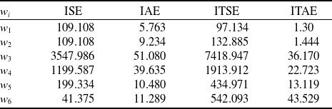
 ${\tilde J_i} = {w_i}{J_i}$
with a positive weighting coefficient
 ${w_i}$
. The weighting coefficients are selected to ensure that the value of
 ${\tilde J_i}$
is approximately equal for each state. Moreover, the same weighting parameters are applied across all objective functions. The weighting coefficients
 ${\omega _1}$
,
 ${\omega _2}$
,
 ${\omega _3}$
,
 ${\omega _4}$
,
 ${\omega _5}$
and
 ${\omega _6}$
correspond to the states
 $x$
,
 $y$
,
 $z$
,
 $\phi $
,
 $\theta $
and
 $\psi $
, respectively. Table 2 provides the values of the weighting coefficients for all states.
The weighting coefficients

6.0 Results
The performance of the cascade flight control system, equipped with PID controllers tuned by the aforementioned optimisation algorithms, is evaluated in simulations designed for the trajectory tracking of a quadcopter. For these optimisation algorithms, the maximum number of iterations, the population size and the lower bound are respectively set to 100, 40 and 0. Conversely, the upper bound is selected within the range of 50 to 100. The values of the remaining parameters, which are set to search for the optimum gains of the PID controllers, are provided in Table 3. These parameters are selected arbitrarily, hence, this parameter setting yields good results rather than the best possible outcomes.
Parameters values of the optimisation algorithms

Simulations are conducted for two distinct flight missions. In the first mission, the quadcopter operates in autonomous flight mode, following a spiral-shaped reference trajectory while maintaining a constant heading. In the second mission, the spiral trajectory is replaced by a rectangular trajectory in the
 $x - y$
plane at a fixed altitude. Initially, the quadcopter ascends to an altitude of 1 m, then proceeds to follow a square trajectory with 1 m sides in the x-y plane. Consequently, the tracking performances of the designed controllers during sharp turns are compared.
6.1 Spiral trajectory tracking mission
The reference position of the quadcopter following the spiral trajectory is defined by the following time-dependent function:
 \begin{align*}x &= {\mathrm{sin}}(t)\\y &= {\mathrm{cos}}(t) - 1\\z &= t\end{align*}
and the heading angle is consistently maintained at
 ${30^ \circ }$
.
Figure 4 illustrates the positions of the quadcopter controlled by the cascade flight control system, with PID coefficients independently tuned using PSO, ABC, GWO and DE optimisation algorithms to minimise the fitness functions. It is evident that the quadcopter successfully follows the reference trajectory in all cases. However, notable differences in the transient response phase are observed due to the effects of the optimisation algorithms. To further analyse these differences, a comprehensive examination of the error evolution is conducted. Figures 5 and 6 display the position and attitude error trajectories, respectively. As indicated, the GWO algorithm yields a less oscillatory response with faster convergence in the transient phase while minimising the IAE and ITAE fitness functions. Conversely, in scenarios employing the ISE and ITSE fitness functions, the DE algorithm provides satisfactory time responses. These outcomes are also reflected in Table 4, which presents the best values of the fitness functions for the spiral trajectory. According to the data in Table 1, the best values of IAE and ITAE are achieved using the GWO, while the DE algorithm produces the best values of ISE and ITSE. These findings are corroborated by the error analysis presented in Table 4.
The best values of the fitness functions for spiral trajectory

Position response of the quadcopter in the spiral trajectory tracking mission with different optimisation algorithms.

Position errors of the quadcopter in the spiral trajectory tracking mission with different optimisation algorithms.

Attitude errors of the quadcopter in the spiral trajectory tracking mission with different optimisation algorithms.

6.2 Square trajectory tracking mission
From the launch position (0,0,0), the quadcopter initially ascends to an altitude of 1m, reaching the coordinates (0,0,1). Subsequently, it moves 1 m along the positive
 $x$
-axis to the coordinates (1,0,1). Following this, the quadcopter travels 1 m along the positive
 $y$
-axis to the coordinate(1,1,1). It then proceeds to move 1 m in the negative
 $x$
-axis direction, arriving at the point (0,1,1). Lastly, it travels 1 m in the negative
 $y$
-axis direction, returning to (0,0,1), where it concludes the movement by maintaining a hover position. Similar to the spiral trajectory, the reference yaw angle (
 $\psi $
) remains constant at 30°. For this mission, the PID optimisation process is reinvoked for all scenarios.
The performance of various PID controllers in tracking the reference square trajectory is assessed by comparing the quadcopter’s position with the predefined trajectory. Figure 7 displays the positions of the quadcopter controlled by PID controllers, each tuned separately by the optimisation algorithms previously employed to minimise four distinct fitness functions. From Fig. 7, it is evident that some PID controllers, such as those tuned by the DE algorithm to minimise the ITAE function and by the PSO algorithm to minimise the IAE function, exhibit unreliable performance for this mission. These observations are further detailed in the error analysis, the results of which are presented in Figs. 8 and 9. While the ABC algorithm minimising the IAE fitness function achieves lower position and attitude errors compared to other algorithms, the GWO algorithm is found to be the most effective for tracking the square trajectory with other fitness functions. Table 5 corroborates these results.
Position response of the quadcopter in the square trajectory tracking mission with different optimisation algorithms.

Position errors of the quadcopter in the square trajectory tracking mission with different optimisation algorithms.

Attitude errors of the quadcopter in the square trajectory tracking mission with different optimisation algorithms.

The best values of the fitness functions for square trajectory

6.3 Robustness against ground effect, mass variation and disturbance
In the previous section, a comprehensive analysis was conducted to evaluate the performance of the meta-heuristic algorithms used to fine-tune PID coefficients, focusing on trajectory-tracking control based on the nonlinear kinematics of the quadcopter. Currently, the robustness of the fine-tuned PID controllers is being tested in simulations. Given the low-altitude flight trajectories of the quadcopter, the ground effect is a significant factor and must be considered. Several approaches to modeling the ground effect have been documented [Reference Cheeseman and Bennett45–Reference Sanchez-Cuevas, Heredia and Ollero48]. Additionally, a linear model has been developed by Wei et al. [Reference Wei, Chan, Lee and Kong49], which is based on experimental results. This linear model is described as follows:
 \begin{align*}\frac{{{u_{{F_{IGE}}}}}}{{{u_F}}} = \left\{ {\begin{array}{l@{\quad}l}{ - 0.0373\frac{z}{R} + 1.1651} & {}{\dfrac{z}{R} \lt 4.42}\\[9pt]1 & {}{{\mathrm{otherwise}}}\end{array}} \right.\end{align*}
In the model,
 $z$
represents the height from the ground,
 $R$
denotes the propeller radius, and
 ${u_{{F_{IGE}}}}$
is the in-ground effect thrust force. Additionally, the flight controller confronts significant challenges from wind disturbances. To achieve accurate trajectory tracking in harsh environments, the flight controller must exhibit robustness against wind disturbances. While unsteady atmospheric conditions pose substantial control challenges at high altitudes, their effects are also non-negligible at very low altitudes, particularly during take-off or payload dropping phases. Consequently, for a more comprehensive analysis of robustness, wind disturbance is incorporated into the nonlinear quadcopter model as external moment disturbances applied to the roll and pitch axes. In the simulations, the following torques are employed [Reference Thanh and Hong50]:
 \begin{align*}{\tau _{{d_\phi }}} = {\tau _{{d_\theta }}} = 7 + 2cos\left( {2\pi t/3} \right)\end{align*}
In the robustness study, two different flight scenarios are considered. In the first scenario, the PID controllers, previously fine-tuned for a spiral path, are tested in the presence of wind disturbances and ground effects. In the second scenario, the quadcopter undertakes a flight mission involving payload transportation. During this mission, the quadcopter, carrying three identical payloads each weighing 200 grams, follows the square route described in the previous section. The quadcopter is programmed to drop one of the payloads at each of the following locations: (1,0,1), (1,1,1), and (0,1,1). This mission also facilitates the investigation of the robustness of the fine-tuned controllers against parameter uncertainty.
6.3.1 Spiral trajectory tracking mission
The total length of the reference spiral trajectory is 42.4 m. The total distances traveled by the quadcopter and the corresponding RMSE values are provided in Table 6. The results reveal that the minimum RMSE and path length values are achieved by the PID controller fine-tuned by the ABC algorithm to minimise the IAE objective function. Figure 10 clearly demonstrates the quadcopter’s capability, controlled by this specific controller, to accurately track the reference spiral trajectory.
Performance of PID controllers for spiral path

6.3.2 Square trajectory tracking mission
This mission is depicted in Fig. 11, with the total path length being 5 m. The total path traveled by the quadcopter and the RMSE errors are summarised in Table 7. The minimum path length and RMSE value are achieved using PID coefficients optimised by the ABC algorithm, which minimised the IAE objective function. As shown in Fig. 12, the PID controller based on the ABC-IAE algorithm demonstrates considerable robustness in the presence of variations in total mass and external disturbances such as ground effect and wind.
Performance of PID controllers for 2
 ${}^{nd}$
Scenario in Fig. 11

Position response of the quadcopter in the spiral trajectory tracking mission with ABC-IAE algorithm.

Reference path for the second scenario.

Position response of the quadcopter with ABC-IAE algorithm for the
 ${2^{{\mathrm{nd}}}}$
scenario.

7.0 Conclusion
This study compares the tracking performances of different PID controllers within a flight control architecture for a quadcopter, which are tuned using various optimisation algorithms: PSO, ABC, GWO and DE. These controllers operate within a bounded search region of interest. The flight control system employs a cascade structure comprising a position controller and an attitude controller, resulting in six PID controllers being finely tuned. During the optimisation process, four distinct weighted fitness functions based on IAE, ISE, ITAE and ITSE performance criteria are utilised.
In the simulations, two different reference trajectories are considered: a spiral trajectory and a square trajectory. The simulation results reveal that the GWO algorithm achieves the minimum values for IAE and ITAE, while the DE algorithm provides the minimum values for ISE and ITSE for the spiral trajectory. For the square trajectory mission, the ABC algorithm delivers the best IAE performance measure. Among the tested algorithms, GWO proves to be the most effective in minimising ISE, ITAE and ITSE performance measures.