
1. Introduction
The initial stage of the laminar–turbulent transition process is known as receptivity (Morkovin Reference Morkovin1969), whereby environmental disturbances transform into perturbations within the boundary layer. Such environmental disturbances can include free-stream noise, vortex structures and surface roughness. Excellent reviews on the receptivity process and boundary layer transition mechanisms are presented by Saric, Reed & Kerschen (Reference Saric, Reed and Kerschen2002) and Saric, Reed & White (Reference Saric, Reed and White2003).
The receptivity process establishes the initial conditions of the boundary layer disturbance, including the disturbance amplitude, frequency and phase. The amplitude of the initial fluctuation dictates the transition path to turbulence. If the initial perturbations are small, the growth (or decay) of the disturbances can be described using linear stability theory. Depending on the geometry of the body and the flow conditions, two- or three-dimensional disturbances may be excited that govern the preliminary stages of the laminar–turbulent transition process. For instance, Tollmien–Schlichting (TS) waves develop on a flat surface or an unswept wing, while cross-flow vortices grow within the boundary layer on a swept wing or rotating disc (von Kármán Reference von Kármán1921; Lingwood & Alfredsson Reference Lingwood and Alfredsson2015). Linear disturbances can be decomposed as
 \begin{equation} \boldsymbol{q}(\boldsymbol{x},t)=A\hat{\boldsymbol{q}}(\boldsymbol{x},t), \end{equation}
where  $\hat {\boldsymbol {q}}$ encompasses the growth (or decay) rate of the perturbation that is governed by the flow conditions, including the Reynolds number of the flow, spatial wavelength and temporal periodicity. (Here
 $\boldsymbol {x}$ represents the spatial coordinates and
 $t$ time.) The disturbance amplitude
 $A$ accounts for the receptivity to the environmental forcing; free-stream effects or surface roughness can vary significantly from one case to another, establishing different disturbance amplitudes that bring about considerable variations in the onset of the latter stages of transition. As the disturbance grows to larger amplitudes, linear stability theory becomes inappropriate, and nonlinear processes and secondary instabilities (amongst other instability mechanisms) emerge that lead to the breakdown of the flow to a turbulent state.
Goldstein (Reference Goldstein1983) identified a receptivity mechanism, whereby an acoustic disturbance (i.e. sound wave) near the leading edge of a flat plate interacts with the flow to establish a TS wave. Another receptivity mechanism was identified independently by Ruban (Reference Ruban1984) and Goldstein (Reference Goldstein1985) that involves a sound wave interacting with a disturbance generated by surface roughness. Following these seminal receptivity investigations, voluminous studies (only a few are cited below) have been undertaken on boundary layer receptivity, including Crouch (Reference Crouch1992a,Reference Crouchb), Choudhari & Streett (Reference Choudhari and Streett1992) and Choudhari (Reference Choudhari1993), who modelled acoustic forcing over a flat plate with surface roughness. Additionally, Wu (Reference Wu2001a,Reference Wub) applied asymptotic theory to distributed and localised roughness in the presence of vortical and acoustic waves.
Choudhari (Reference Choudhari1994) modelled the receptivity of swept wing boundary layers (Falkner–Skan–Cooke flows), whereby stationary and non-stationary cross-flow vortices were excited by a spanwise-periodic roughness distribution. Using a compressible linearised Navier–Stokes solver, Collis & Lele (Reference Collis and Lele1999) found that surface curvature and non-parallel effects played a significant role in the receptivity process along the leading edge of a swept wing. Later, Schrader and co-workers modelled the receptivity of a swept wing leading edge by coupling free-stream turbulence and surface roughness (Schrader, Brandt & Henningson Reference Schrader, Brandt and Henningson2009; Schrader, Amin & Brandt Reference Schrader, Amin and Brandt2010).
Several experiments on a swept wing were undertaken by the Saric group, in which cross-flow disturbances were excited by localised roughness elements (Reibert et al. Reference Reibert, Saric, Carillo and Chapman1996; Saric, Carrillo & Reibert Reference Saric, Carrillo and Reibert1998; Radeztsky, Reibert & Saric Reference Radeztsky, Reibert and Saric1999). In particular, it was noted by Radeztsky et al. (Reference Radeztsky, Reibert and Saric1999) that receptivity is most enhanced by roughness elements located near the onset of unstable behaviour. Numerical methods were employed by Ng & Crouch (Reference Ng and Crouch1999) in an attempt to replicate the Saric experiments. Using a local parallel flow assumption, they obtained qualitatively similar results as that found experimentally. More recently, Tempelmann et al. (Reference Tempelmann, Schrader, Hanifi, Brandt and Henningson2012b) employed direct numerical simulations (DNS) and parabolised stability equations (PSE) to study the receptivity of a swept wing to localised roughness elements, with the objective to reproduce the wind tunnel experiments performed by the Saric group. In all cases modelled, DNS and PSE cross-flow amplitudes were smaller than the equivalent experimental disturbance measurements. It was suggested that uncertainties in the experimental set-up were possibly responsible for these differences.
This paper is concerned with the receptivity of the rotating disc boundary layer to randomly distributed surface roughness, which is the archetypal model for the study of three-dimensional instability mechanisms that trigger laminar–turbulent transition. The flow on a rotating disc is formed when a planar solid surface is rotated, with a constant angular velocity, that drives the motion of the otherwise still fluid immediately above it. This particular flow has been of fundamental interest to the fluid dynamics community throughout much of the twentieth and twenty-first centuries, with the foundational study undertaken by von Kármán (Reference von Kármán1921). A review by Lingwood & Alfredsson (Reference Lingwood and Alfredsson2015) provides an extensive overview of the numerous investigations that have been carried out on the rotating disc using theoretical, numerical and experimental methods. The seminal experimental and theoretical study by Gregory, Stuart & Walker (Reference Gregory, Stuart and Walker1955) revealed that the inviscid cross-flow instability appears as stationary spiral vortices on the rotating disc. In addition to cross-flow disturbances, the rotating disc is susceptible to at least two other forms of instability. The first of these instabilities is viscous and is a direct consequence of the Coriolis forces present in rotating boundary layers (Faller & Kaylor Reference Faller and Kaylor1966; Malik Reference Malik1986), while the second instability is a spatially damped mode that propagates radially inwards (Mack Reference Mack1985).
In their china-clay visualisation experiments, Gregory et al. (Reference Gregory, Stuart and Walker1955) observed cross-flow disturbances as 28–32 vortices that spiralled radially outwards at an angle of  $14^\circ$. The number of cross-flow vortices is directly related to the integer-valued azimuthal mode number
 $n$ that represents the periodicity of the disturbance in the azimuthal direction. Similar observations were made in later experimental studies by Kobayashi, Kohama & Takamadate (Reference Kobayashi, Kohama and Takamadate1980), Malik, Wilkinson & Orszag (Reference Malik, Wilkinson and Orszag1981), Kohama (Reference Kohama1984) and Wilkinson & Malik (Reference Wilkinson and Malik1985). The onset of these stationary cross-flow vortices was observed experimentally for a Reynolds number
 $Re_c<300$ (Kobayashi et al. Reference Kobayashi, Kohama and Takamadate1980; Malik et al. Reference Malik, Wilkinson and Orszag1981) and confirmed as
 $Re_c\approx 286$ using linear stability theory by Malik et al. (Reference Malik, Wilkinson and Orszag1981) and Lingwood (Reference Lingwood1995), amongst many others. Moreover, Siddiqui et al. (Reference Siddiqui, Mukund, Scott and Pier2013) observed that those stationary perturbations with an azimuthal mode number near
 $n=30$ developed with the largest spatial growth. (A formal definition for the Reynolds number
 $Re$ is given below in (2.7).)
An absolute form of instability was discovered by Lingwood (Reference Lingwood1995) using the Briggs (Reference Briggs1964) pinch-point criterion, and was shown to result from the coalescence of the cross-flow instability (Gregory et al. Reference Gregory, Stuart and Walker1955) and the spatially damped mode found by Mack (Reference Mack1985). More dangerous than the convectively unstable cross-flow mode, Lingwood (Reference Lingwood1995) identified the critical Reynolds number for absolute instability as  $Re_a=510$ (later corrected to
 $Re_a=507$ by Lingwood Reference Lingwood1997) for an azimuthal mode number
 $n=68$. The linear stability analysis undertaken by Lingwood (Reference Lingwood1995) was based on a local theory, which was achieved by imposing a spatially homogeneous flow approximation. This is often termed the parallel flow approximation, whereby the radial dependence of the base flow is ignored.
Davies & Carpenter (Reference Davies and Carpenter2003) undertook a numerical investigation of the radially dependent inhomogeneous flow over an infinite rotating disc and showed that absolute instability was not sufficient for a disturbance to become globally linearly unstable. Instead, for azimuthal mode numbers  $n$ near the critical conditions for absolute instability, convective characteristics dominated the global disturbance development. However, a subsequent study by Thomas & Davies (Reference Thomas and Davies2018) found that a form of global linear instability can occur, although such behaviour only arises for azimuthal mode numbers significantly greater than that associated with the onset of absolute instability that were the primary focus of the earlier investigation. While absolute instability is a necessary condition for the onset of global linear instability to occur, it is not a sufficient condition. Generally, the region of absolute instability must exceed some threshold size for global linear instability to ensue (Chomaz, Huerre & Redekopp Reference Chomaz, Huerre and Redekopp1988; Huerre & Monkewitz Reference Huerre and Monkewitz1990). In particular, for the flow on a rotating disc, the radial extent of absolute instability increases as the azimuthal mode number
 $n$ increases. Thomas & Davies (Reference Thomas and Davies2018) found that, for
 $n\gtrapprox 83$, globally linearly unstable behaviour emerges that is characterised by a stronger than exponential temporal growth. Furthermore, Thomas and Davies utilised solutions of the Ginzburg–Landau equation (Hunt & Crighton Reference Hunt and Crighton1991) to show that the onset of global linear instability can be predicted using local stability characteristics based on the homogeneous flow approximation. The results of Thomas and Davies indicate that the infinite rotating disc is stable for small Reynolds numbers
 $Re$ and azimuthal mode numbers
 $n$. For larger
 $Re$ and
 $n$, regions of local convective instability (such as cross-flow vortices) and absolute instability emerge, but globally linearly unstable behaviour only develops for sufficiently large azimuthal mode numbers. Further studies have shown that this behaviour is ubiquitous across the family of rotating boundary layers, including cones in a quiescent medium and discs with roughness modelled via the partial-slip boundary condition (Thomas & Davies Reference Thomas and Davies2019; Thomas, Stephen & Davies Reference Thomas, Stephen and Davies2020).
Experimental observations indicate that transition to turbulence in the rotating disc boundary layer is highly reproducible with Reynolds numbers  $500\leqslant {\textit {Re}} \leqslant 566$ quoted in the literature. For instance, Gregory et al. (Reference Gregory, Stuart and Walker1955) observed transition for
 ${\textit {Re}}=533$, while Malik et al. (Reference Malik, Wilkinson and Orszag1981) and Kobayashi et al. (Reference Kobayashi, Kohama and Takamadate1980) indicate that transition sets in for
 $513<{\textit {Re}}<526$ and
 ${\textit {Re}}=566$, respectively. More recently, Lingwood (Reference Lingwood1996) suggests that transition on a clean disc occurs for Reynolds numbers
 ${\textit {Re}}=513\pm 3\,\%$, while Othman & Corke (Reference Othman and Corke2006) observed transition about
 ${\textit {Re}}=539$. A comprehensive list of the many experimental investigations undertaken on the rotating disc and transition Reynolds numbers is given by Imayama, Alfredsson & Lingwood (Reference Imayama, Alfredsson and Lingwood2013); see table 1 of their paper.
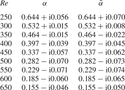
Linear and adjoint radial wavenumbers,  $\alpha$ and
 $\tilde {\alpha }$, for the azimuthal mode number
 $n=32$, determined by applying the homogeneous flow approximation.

Since absolute instability and transition to turbulence occur within the same band of Reynolds numbers, Lingwood (Reference Lingwood1996) suggested that the absolutely unstable mechanism is the primary cause for the breakdown of the laminar flow. Several recent investigations on a rotating disc of finite radius suggest that absolute instability can establish globally unstable behaviour if disc edge effects are accounted for (Healey Reference Healey2010; Imayama et al. Reference Imayama, Alfredsson and Lingwood2013; Pier Reference Pier2013; Appelquist et al. Reference Appelquist, Schlatter, Alfredsson and Lingwood2015, Reference Appelquist, Schlatter, Alfredsson and Lingwood2016; Lee et al. Reference Lee, Nishio, Izawa and Fukunishi2017, Reference Lee, Nishio, Izawa and Fukunishi2018). Additionally, Pier (Reference Pier2003) suggests that a secondary absolute instability develops near the primary absolute instability, providing an alternative route to turbulence. Meanwhile, the discovery by Thomas & Davies (Reference Thomas and Davies2018) that a form of global linear instability develops for sufficiently large azimuthal mode numbers  $n$ may provide additional support to Lingwood's conclusions. However, there does not appear to be any evidence for these large
 $n$ modes in the available experimental literature. This does not imply that these globally unstable disturbances do not exist, but that other faster growing instabilities (such as the cross-flow instability) may prevent their development. Cross-flow disturbances (both stationary and travelling) grow rapidly and can achieve exponential growth factors
 $N \in [7:11]$ within the range of Reynolds numbers that transition is observed experimentally (Thomas & Davies Reference Thomas and Davies2018). Hence, cross-flow vortices may still be the primary mechanism for laminar–turbulent transition in the rotating disc boundary layer.
Imayama et al. (Reference Imayama, Alfredsson and Lingwood2013) remark that the onset of transition in experiments is dependent on the definition for transition. For instance, Lingwood (Reference Lingwood1996) based her observations for transition on the onset of nonlinearity, while Othman & Corke (Reference Othman and Corke2006) based it on the deformation of the laminar flow profile. (Table 3 of Imayama et al. (Reference Imayama, Alfredsson and Lingwood2013) provides an overview of the interpretations for transition in experiments.) Nevertheless, independent of the definition for transition, there is a clear and marked region on the disc that transition occurs. Additionally, it is very difficult to eliminate stationary cross-flow vortices in experiments, even for the flow over a polished disc; unavoidable surface roughness will inevitably excite stationary cross-flow disturbances (Imayama, Alfredsson & Lingwood Reference Imayama, Alfredsson and Lingwood2016). Thus, the route to transition is dependent on the roughness height. Wilkinson & Malik (Reference Wilkinson and Malik1985) found that transition occurred for  $521<{\textit {Re}}<530$ on a rough disc, while transition on a clean disc was delayed to
 $543<{\textit {Re}}<556$. Imayama et al. (Reference Imayama, Alfredsson and Lingwood2016) experimentally modelled surface roughness effects, whereby artificial roughness elements were placed on the surface of an otherwise clean disc. As expected, transition occurred earlier on the rough disc, with very little surface roughness needed to trigger the strong growth of unstable stationary cross-flow disturbances. Thus, transition occurred via a convective route. However, in addition to the stationary cross-flow instability, travelling disturbances were observed on the clean disc. It was suggested that this is evidence for absolute instability, and thus, transition to turbulence occurs via an absolute route. On the other hand, Appelquist et al. (Reference Appelquist, Schlatter, Alfredsson and Lingwood2018) numerically excited stationary cross-flow disturbances via surface roughness elements of variable amplitude, and traced their development through the linear stage, nonlinear saturation and finally transition to turbulence. In all instances simulated, the primary instability was convectively unstable, before nonlinear effects and secondary instabilities formed.
In experimental apparatus, a disc is deemed to be rough when an artificial roughness is fixed to the disc surface. A disc is then described as clean if it is polished to a certain threshold level. In Othman & Corke (Reference Othman and Corke2006) the disc surface was polished to a  $2 \ \mathrm {\mu }\textrm {m}$ finish, while the natural surface roughness was less than
 $1\ \mathrm {\mu }\textrm {m}$ in Imayama, Alfredsson & Lingwood (Reference Imayama, Alfredsson and Lingwood2012), Imayama et al. (Reference Imayama, Alfredsson and Lingwood2013), Imayama, Alfredsson & Lingwood (Reference Imayama, Alfredsson and Lingwood2014) and Imayama et al. (Reference Imayama, Alfredsson and Lingwood2016). However, even for clean discs natural surface roughness still occurs and will inevitably excite stationary cross-flow disturbances, albeit at a lower initial amplitude. Furthermore, the size and shape of the roughness will be specific to each disc, leading to both different receptivity amplitudes and routes to turbulence. Quantifying this effect and computing the receptivity amplitude can be computationally expensive using the linear Navier–Stokes (LNS) equations. Indeed, computing mean receptivity characteristics for predicting the possible transition scenarios would require the LNS equations to be solved for many roughness realisations. Thus, the computational demands of an LNS based receptivity analysis can quickly escalate. However, such difficulties can be overcome using an adjoint based approach.
The adjoint linearised Navier–Stokes (ALNS) equations are both computationally and economically more efficient than other receptivity formulations (such as the LNS equations). They only require solutions to the LNS and ALNS equations to be computed once, after which they can be used to instantaneously predict the amplitude of the disturbance excited by many forms of external forcing. Hill (Reference Hill1995) derived the ALNS equations for the two-dimensional Blasius boundary layer and determined the sensitivity of TS waves. Later, Airiau (Reference Airiau2000) extended Hill's analysis to include non-parallel effects, while Dobrinsky & Collis (Reference Dobrinsky and Collis2000) and Dobrinsky (Reference Dobrinsky2002) employed adjoint methods to compute the receptivity of the family of Falkner–Skan flows. Adjoint formulations have been applied to many other flow systems and boundary layer instabilities (Luchini & Bottaro Reference Luchini and Bottaro1998; Pralits, Hanifi & Henningson Reference Pralits, Hanifi and Henningson2002; Pralits & Hanifi Reference Pralits and Hanifi2003; Giannetti & Luchini Reference Giannetti and Luchini2006; Carpenter et al. Reference Carpenter, Choudhari, Li, Streett and Chang2010; Tempelmann, Hanifi & Henningson Reference Tempelmann, Hanifi and Henningson2012a), with a review given by Luchini & Bottaro (Reference Luchini and Bottaro2014).
Thomas, Mughal & Ashworth (Reference Thomas, Mughal and Ashworth2017) derived the compressible ALNS equations for the flow over a swept wing and undertook a Monte-Carlo type uncertainty quantification analysis. Many thousands of roughness distributions were randomly generated and the amplitude of stationary cross-flow vortices was computed to ascertain mean receptivity characteristics. Similar studies were undertaken by Mughal & Ashworth (Reference Mughal and Ashworth2013) and Raposo, Mughal & Ashworth (Reference Raposo, Mughal and Ashworth2018) using an LNS scheme.
In this investigation we derive for the first time, the ALNS equations in cylindrical coordinates for the rotating disc boundary layer. An extensive receptivity study is undertaken, whereby stationary cross-flow vortices are established by many randomly generated surface roughnesses. Mean receptivity characteristics, based on the root-mean-square (r.m.s.) of the surface roughness, are then used to predict the radial location that the stationary cross-flow instability attains amplitudes sufficient to invalidate the linear stability assumptions and bring about nonlinear effects and the latter stages of the laminar–turbulent transition process.
The remainder of this paper is outlined as follows. In the subsequent section the undisturbed flow is described. In § 3 the ALNS equations in cylindrical coordinates are derived. The velocity–vorticity form of the ALNS equations are presented in § 4 based on the formulation of Davies & Carpenter (Reference Davies and Carpenter2001). The receptivity of the rotating disc boundary layer to surface roughness is discussed in § 5, with conclusions given in § 6.
2. Undisturbed flow
A disc of infinite radius rotates beneath an infinite body of incompressible fluid at a constant angular velocity  $\varLambda ^*$ about the vertical axis that passes through the centre of the disc. The modelling is carried out in cylindrical polar coordinates, where
 $r^*$,
 $\theta$ and
 $z^*$ denote the radial, azimuthal and wall-normal directions, respectively. (Here an asterisk denotes dimensional quantities.) In what follows, all quantities are defined in the frame of reference that rotates with the disk.
The Navier–Stokes equations, in cylindrical coordinates, are defined as
 \begin{align} \dfrac{\partial U_r^*}{\partial t^*} +(\boldsymbol{U^*}\boldsymbol{\cdot}\boldsymbol{\nabla}^*)U_r^* -\dfrac{U_{\theta}^{*2}}{r^*}-2\varLambda^*U_{\theta}^*-\varLambda^{*2}r^* & ={-}\dfrac{1}{\rho^*}\frac{\partial P^*}{\partial r^*} \nonumber\\ &\quad + \nu^* \left(\boldsymbol{\nabla}^{*2}U_r^*-\dfrac{U_r^*}{r^{*2}}-\dfrac{2}{r^{*2}}\dfrac{\partial U_\theta^*}{\partial \theta}\right), \end{align}
 \begin{align} \dfrac{\partial U_\theta^*}{\partial t^*} +(\boldsymbol{U^*}\boldsymbol{\cdot}\boldsymbol{\nabla}^*)U_\theta^* + \dfrac{U_{\theta}^*U_r^*}{r^*}+ 2\varLambda^*U_{r}^*& ={-}\dfrac{1}{r^*\rho^*}\dfrac{\partial P^*}{\partial \theta} \nonumber\\ &\quad + \nu^* \left(\boldsymbol{\nabla}^{*2}U_\theta^*-\dfrac{U_\theta^*}{r^{*2}}+\frac{2}{r^{*2}}\dfrac{\partial U_r^*}{\partial \theta}\right), \end{align}
 \begin{gather} \dfrac{\partial U_z^*}{\partial t^*} +(\boldsymbol{U^*}\boldsymbol{\cdot}\boldsymbol{\nabla}^*)U_z^*={-}\dfrac{1}{\rho^*}\dfrac{\partial P^*}{\partial z^*} + \nu^* \boldsymbol{\nabla}^{*2}U_z^*, \end{gather}
 \begin{gather} \dfrac{1}{r^*}\dfrac{\partial(r^*U_r^*)}{\partial r^*}+\dfrac{1}{r^*}\dfrac{\partial U_{\theta}^*}{\partial \theta}+\dfrac{\partial U_z^*}{\partial z^*}=0, \end{gather}
where
 \begin{equation} \boldsymbol{U^*}\boldsymbol{\cdot}\boldsymbol{\nabla}^*=U_r^*\dfrac{\partial}{\partial r^*}+\dfrac{U_{\theta}^*}{r^*}\dfrac{\partial}{\partial \theta}+U_z^*\dfrac{\partial}{\partial z^*} \end{equation}
and
 \begin{equation} \boldsymbol{\nabla}^{*2} = \dfrac{\partial^2 }{\partial r^{*2}} +\dfrac{1}{r^*}\dfrac{\partial }{\partial r^*}+\dfrac{1}{r^{*2}}\dfrac{\partial^2}{\partial \theta^2}+\dfrac{\partial^2}{\partial z^{*2}}.\end{equation}
The kinematic viscosity and density of the fluid are denoted by  $\nu ^*$ and
 $\rho *$, while
 $\boldsymbol {U}^* = (U_r^*,U_{\theta }^*,U_z^*)$ and
 $P^*$ represent the respective dimensional velocity and pressure fields. Boundary conditions on the disc surface are defined as
 \begin{equation} U_r^*=U_{\theta}^*=U_z^*=0 \quad \textrm{on} \ z^*=0, \end{equation}
and in the far field
 \begin{equation} U_r^* \rightarrow 0 \quad \textrm{and} \quad U_{\theta}^* \rightarrow - r^*\varLambda^* \quad \text{as} \ z^* \rightarrow \infty. \end{equation}
The undisturbed flow field is established using the von Kármán (Reference von Kármán1921) similarity variables
 \begin{equation} \boldsymbol{U}^*= \left( r^*\varLambda^*F(z), r^*\varLambda^*G(z), \delta^*\varLambda^*H(z)\right)\quad \textrm{and} \quad P^*=\rho^*\nu^*\varLambda^*P(z), \end{equation}
where  $F$,
 $G$ and
 $H$ represent the non-dimensional velocity profiles along the three coordinate directions. The non-dimensional pressure field is denoted
 $P$ and
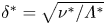 $\delta ^*=\sqrt {\nu ^*/\varLambda ^*}$ represents the constant boundary layer thickness used here to scale units of length:
 $r = r^*/\delta ^*$ and
 $z=z^*/\delta ^*$. On substituting (2.4) into the Navier–Stokes equations (2.1), the following system of ordinary differential equations for
 $F$,
 $G$,
 $H$ and
 $P$ is derived,
 $$\begin{gather} F'' = F^2+F'H-(G+1)^2, \end{gather}$$
 $$\begin{gather}G'' = 2F(G+1)+G'H, \end{gather}$$
 $$\begin{gather}H'' = P'+HH', \end{gather}$$
 $$\begin{gather}0 = 2F+H', \end{gather}$$
which is solved subject to the boundary conditions
 \begin{equation} F=G=H=0 \quad \textrm{on} \ z=0 \end{equation}
and
 \begin{equation} F\rightarrow 0 \quad \textrm{and} \quad G\rightarrow -1 \quad \textrm{as} \ z\rightarrow\infty. \end{equation}
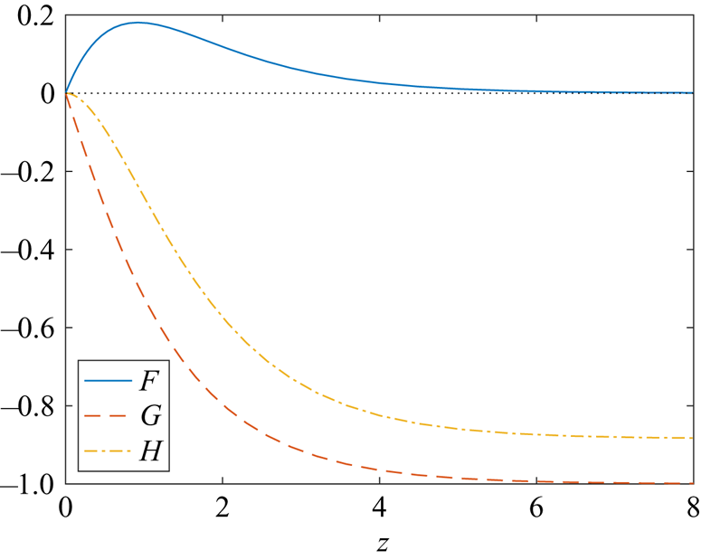
A prime denotes differentiation with respect to  $z$. Figure 1 depicts the von Kármán velocity profiles
 $F$,
 $G$ and
 $H$ as functions of the wall-normal
 $z$-direction.
The von Kármán velocity profiles  $F$,
 $G$ and
 $H$.

Non-dimensionalising velocity and pressure on the respective scales  $r_o^*\varLambda ^*$ and
 $\rho ^*r_o^{*2}\varLambda ^{*2}$, the non-dimensional undisturbed velocity and pressure fields are given as
 \begin{equation} \boldsymbol{U}_{\boldsymbol{B}}(r,z)=\left(\frac{r}{{\textit{Re}}}F(z), \frac{r}{{\textit{Re}}}G(z), \frac{1}{{\textit{Re}}}H(z) \right) \quad \textrm{and} \quad P_B(z)=\frac{1}{{\textit{Re}}^2}P(z), \end{equation}
where the Reynolds number is defined as
 \begin{equation} {\textit{Re}}=r_o^*/\delta^*\equiv r_o,\end{equation}
for a non-dimensional reference radius  $r_o$.
3. Derivation of the ALNS equations
3.1. Linearised Navier–Stokes equations
The undisturbed flow (2.6) is perturbed by infinitesimally small disturbances, with the total velocity  $\boldsymbol {U}$ and pressure
 $P$ given as
 \begin{equation} \boldsymbol{U}=\boldsymbol{U}_{\boldsymbol{B}}+\boldsymbol{u}, \quad P=P_B+p, \end{equation}
where the velocity perturbation  $\boldsymbol {u}=(u_r,u_{\theta },u_z).$ Substituting (3.1) into the Navier–Stokes equations and linearising with respect to the perturbation
 $\boldsymbol {q}=(\boldsymbol {u},p)$ gives the LNS system of equations
 \begin{align} L_r(\boldsymbol{q};\boldsymbol{U}_{\boldsymbol{B}},{\textit{Re}}) &= \frac{\partial u_r}{\partial t}+\frac{rF}{{\textit{Re}}}\frac{\partial u_r}{\partial r}+\frac{F}{{\textit{Re}}}u_r+\frac{G}{{\textit{Re}}}\frac{\partial u_r}{\partial\theta}+\frac{H}{{\textit{Re}}}\frac{\partial u_r}{\partial z}+\frac{rF'}{{\textit{Re}}}u_z \nonumber\\ &\quad -\frac{2(G+1)}{{\textit{Re}}}u_{\theta} +\dfrac{\partial p}{\partial r}-\frac{1}{{\textit{Re}}}\left( \left(\nabla^2 - \frac{1}{r^2} \right) u_r - \frac{2}{r^2}\dfrac{\partial u_{\theta}}{\partial\theta} \right) = 0, \end{align}
 \begin{align} L_{\theta}(\boldsymbol{q};\boldsymbol{U}_{\boldsymbol{B}},{\textit{Re}}) &= \frac{\partial u_{\theta}}{\partial t}+\frac{rF}{{\textit{Re}}}\frac{\partial u_{\theta}}{\partial r}+\frac{F}{{\textit{Re}}}u_{\theta}+\frac{G}{{\textit{Re}}}\frac{\partial u_{\theta}}{\partial\theta}+\frac{H}{{\textit{Re}}}\frac{\partial u_{\theta}}{\partial z}+\frac{rG'}{{\textit{Re}}}u_z \nonumber\\ &\quad +\frac{2(G+1)}{{\textit{Re}}}u_r +\frac{1}{r}\dfrac{\partial p}{\partial \theta}-\frac{1}{{\textit{Re}}}\left( \left(\nabla^2 - \frac{1}{r^2} \right) u_{\theta} + \frac{2}{r^2}\dfrac{\partial u_r}{\partial\theta} \right)=0, \end{align}
 \begin{align} L_z(\boldsymbol{q};\boldsymbol{U}_{\boldsymbol{B}},{\textit{Re}}) &= \frac{\partial u_z}{\partial t}+\frac{rF}{{\textit{Re}}}\frac{\partial u_z}{\partial r}+\frac{G}{{\textit{Re}}}\frac{\partial u_z}{\partial\theta}+\frac{H}{{\textit{Re}}}\frac{\partial u_z}{\partial z}+\frac{H'}{{\textit{Re}}}u_z+\dfrac{\partial p}{\partial z}-\frac{1}{{\textit{Re}}}\nabla^2u_z=0,\end{align}
 \begin{gather} \frac{1}{r}\frac{\partial(ru_r)}{\partial r}+\frac{1}{r}\frac{\partial u_{\theta}}{\partial\theta}+\frac{\partial u_z}{\partial z}=0, \end{gather}
where  $\nabla ^2$ is the non-dimensional form of (2.2b). For convenience, we introduce the LNS operator
 $\boldsymbol {L}=(L_r,L_{\theta },L_z)$.
The corresponding boundary conditions on the disc surface and in the far field are respectively given as
 \begin{equation} \boldsymbol{u}=\boldsymbol{0} \quad \textrm{on} \quad z=0 \quad \textrm{and} \quad \boldsymbol{u}\rightarrow\boldsymbol{0} \quad \textrm{as} \ z\rightarrow \infty. \end{equation}
3.2. Adjoint linearised Navier–Stokes equations
Formulating the Lagrange identity is key to deriving the ALNS system of equations. This is achieved by first introducing adjoint velocity  $\tilde {\boldsymbol {u}}=(\tilde {u}_r,\tilde {u}_{\theta },\tilde {u}_z)$ and pressure
 $\tilde {p}$ perturbation fields. The Lagrange identity is then derived by taking the inner product of the LNS equations (3.2) with
 $\tilde {\boldsymbol {q}}=(\boldsymbol {\tilde {u}},\tilde {p})$, and integrating by parts to give
 \begin{align}
&\underbrace{\boldsymbol{L}(\boldsymbol{q};\boldsymbol{U}_{\boldsymbol{B}},{\textit{Re}})
\boldsymbol{\cdot}\tilde{\boldsymbol{u}}+\boldsymbol{\nabla}\boldsymbol{\cdot}\boldsymbol{u}\tilde{p}}_{\text{Inner
product of LNS }\&
\tilde{\boldsymbol{q}}}+\underbrace{\boldsymbol{u}\boldsymbol{\cdot}\tilde{\boldsymbol{L}}(
\tilde{\boldsymbol{q}};\boldsymbol{U}_{\boldsymbol{B}},{\textit{Re}})+p\boldsymbol{\nabla}\boldsymbol{\cdot}
\tilde{\boldsymbol{u}}}_{\text{Inner product of ALNS }\&
\boldsymbol{q}}
\nonumber\\ &\quad =\underbrace{\frac{\partial}{\partial
t}(\boldsymbol{u}\boldsymbol{\cdot}\tilde{\boldsymbol{u}})+\boldsymbol{\nabla}\boldsymbol{\cdot}
\boldsymbol{J}(\boldsymbol{q},\tilde{\boldsymbol{q}})}_{\text{Bilinear concomitant}},
\end{align}
where
 \begin{equation} \boldsymbol{u}\boldsymbol{\cdot}\tilde{\boldsymbol{u}}=u_r\tilde{u}_r+u_{\theta}\tilde{u}_{\theta}+u_z\tilde{u}_z. \end{equation}
(Note that the integration along the radial direction is performed on a finite interval.)
The ALNS system of equations are then given by those expressions above the second underbrace in (3.4) that form an inner product with the linear perturbation  $\boldsymbol {q}=(\boldsymbol {u},p)$,
 \begin{align} \tilde{L}_r(\tilde{\boldsymbol{q}};\boldsymbol{U}_{\boldsymbol{B}},{\textit{Re}}) &= \frac{\partial \tilde{u}_r}{\partial t}+\frac{rF}{{\textit{Re}}}\frac{\partial \tilde{u}_r}{\partial r}-\frac{F}{{\textit{Re}}}\tilde{u}_{r}+\frac{G}{{\textit{Re}}}\frac{\partial \tilde{u}_r}{\partial\theta}+\frac{H}{{\textit{Re}}}\frac{\partial \tilde{u}_r}{\partial z} \nonumber\\ &\quad-\frac{2(G+1)}{{\textit{Re}}}\tilde{u}_{\theta} + \frac{\partial \tilde{p}}{\partial r}+\frac{1}{{\textit{Re}}}\left( \left(\nabla^2 - \frac{1}{r^2} \right) \tilde{u}_r - \frac{2}{r^2}\frac{\partial \tilde{u}_{\theta}}{\partial\theta} \right)=0, \end{align}
 \begin{align} \tilde{L}_{\theta}(\tilde{\boldsymbol{q}};\boldsymbol{U}_{\boldsymbol{B}},{\textit{Re}}) &= \frac{\partial \tilde{u}_{\theta}}{\partial t}+\frac{rF}{{\textit{Re}}}\frac{\partial \tilde{u}_{\theta}}{\partial r}-\frac{F}{{\textit{Re}}}\tilde{u}_{\theta}+\frac{G}{{\textit{Re}}}\frac{\partial \tilde{u}_{\theta}}{\partial\theta}+\frac{H}{{\textit{Re}}}\frac{\partial \tilde{u}_{\theta}}{\partial z} \nonumber\\ &\quad +\frac{2(G+1)}{{\textit{Re}}}\tilde{u}_{r} + \frac{1}{r}\frac{\partial \tilde{p}}{\partial \theta}+\frac{1}{{\textit{Re}}}\left( \left(\nabla^2 - \frac{1}{r^2} \right) \tilde{u}_{\theta} + \frac{2}{r^2}\frac{\partial \tilde{u}_r}{\partial\theta}\right)=0, \end{align}
 \begin{align} \tilde{L}_z(\tilde{\boldsymbol{q}};\boldsymbol{U}_{\boldsymbol{B}},{\textit{Re}}) &= \frac{\partial \tilde{u}_z}{\partial t}+\frac{rF}{{\textit{Re}}}\frac{\partial \tilde{u}_z}{\partial r}+\frac{G}{{\textit{Re}}}\frac{\partial \tilde{u}_z}{\partial\theta}+\frac{H}{{\textit{Re}}}\frac{\partial \tilde{u}_z}{\partial z}-\frac{rF'}{{\textit{Re}}}\tilde{u}_{r} \nonumber\\ &\quad -\frac{rG'}{{\textit{Re}}}\tilde{u}_{\theta}-\frac{H'}{{\textit{Re}}}\tilde{u}_{z}+\frac{\partial \tilde{p}}{\partial z}+\frac{1}{{\textit{Re}}}\nabla^2\tilde{u}_z=0, \end{align}
 \begin{equation} \frac{1}{r}\frac{\partial(r\tilde{u}_r)}{\partial r}+\frac{1}{r}\frac{\partial \tilde{u}_{\theta}}{\partial\theta}+\frac{\partial \tilde{u}_z}{\partial z}=0,\end{equation}
where the ALNS operator  $\tilde {\boldsymbol {L}}=(\tilde {L}_r,\tilde {L}_{\theta },\tilde {L}_z)$. Note that the viscous terms in the ALNS equations (3.6) are of the opposite sign to the equivalent terms in the LNS equations (3.2). Thus, the adjoint equations must be solved backwards in time.
The system of ALNS equations (3.6) are solved subject to an equivalent set of boundary conditions as imposed on the LNS system of equations (3.2),
 \begin{equation} \tilde{\boldsymbol{u}}=\boldsymbol{0} \quad \textrm{on} \quad z=0 \quad \textrm{and} \quad \tilde{\boldsymbol{u}}\rightarrow\boldsymbol{0} \quad \textrm{as} \ z\rightarrow \infty. \end{equation}
3.3. Bilinear concomitant
The operator  $\boldsymbol {J}=(J_r,J_{\theta },J_z)$, on the right-hand side of the Lagrange identity (3.4), represents the bilinear concomitant and is defined as
 \begin{align} J_r(\boldsymbol{q},\tilde{\boldsymbol{q}})&=\frac{rF}{{\textit{Re}}}\boldsymbol{u} \boldsymbol{\cdot}\tilde{\boldsymbol{u}}+p\tilde{u}_r+u_r\tilde{p}\nonumber\\ &\quad +\frac{1}{{\textit{Re}}}\left(u_r\frac{\partial\tilde{u}_r}{\partial r}-\tilde{u}_r\frac{\partial u_r}{\partial r}+u_{\theta}\frac{\partial\tilde{u}_{\theta}}{\partial r}-\tilde{u}_{\theta}\frac{\partial u_{\theta}}{\partial r}+u_z\frac{\partial\tilde{u}_z}{\partial r}-\tilde{u}_z\frac{\partial u_z}{\partial r}\right), \end{align}
 \begin{align} J_{\theta}(\boldsymbol{q},\tilde{\boldsymbol{q}})&=\frac{rG}{{\textit{Re}}}\boldsymbol{u}\boldsymbol{\cdot}\tilde{\boldsymbol{u}}+p\tilde{u}_{\theta}+u_{\theta}\tilde{p}\nonumber\\ &\quad+\frac{1}{r{\textit{Re}}}\left(u_r\frac{\partial\tilde{u}_r}{\partial \theta}-\tilde{u}_r\frac{\partial u_r}{\partial \theta}+u_{\theta}\frac{\partial\tilde{u}_{\theta}}{\partial \theta}-\tilde{u}_{\theta}\frac{\partial u_{\theta}}{\partial \theta}+u_z\frac{\partial\tilde{u}_z}{\partial \theta}\right.\nonumber\\ &\left.\quad -\tilde{u}_z\frac{\partial u_z}{\partial \theta} + 2 \left(u_{\theta}\tilde{u}_r-u_r\tilde{u}_{\theta}\right)\right), \end{align}
 \begin{align} J_z(\boldsymbol{q},\tilde{\boldsymbol{q}})&=\frac{H}{{\textit{Re}}}\boldsymbol{u}\boldsymbol{\cdot} \tilde{\boldsymbol{u}}+p\tilde{u}_z+u_z\tilde{p}\nonumber\\ &\quad +\frac{1}{{\textit{Re}}}\left(u_r\frac{\partial\tilde{u}_r}{\partial z}-\tilde{u}_r\frac{\partial u_r}{\partial z}+u_{\theta}\frac{\partial\tilde{u}_{\theta}}{\partial z}-\tilde{u}_{\theta}\frac{\partial u_{\theta}}{\partial z}+u_z\frac{\partial\tilde{u}_z}{\partial z}-\tilde{u}_z\frac{\partial u_z}{\partial z}\right). \end{align}
In the subsequent analysis, the  $\boldsymbol {J}$-operator is utilised to establish a formula for predicting the receptivity amplitude of the stationary cross-flow instability excited by surface roughness.
3.4. Normalisation
Stationary cross-flow perturbations  $\boldsymbol {q}=(\boldsymbol {u},p)$ are assumed to be linear, infinitesimally small and of the general form
 \begin{equation} \boldsymbol{q}(r,\theta,z,t) = \hat{\boldsymbol{q}}(r,z) \mathrm{e}^{\textrm{i}n\theta} \end{equation}
for an integer-valued azimuthal mode number  $n$. Similarly, stationary adjoint perturbations
 $\tilde {\boldsymbol {q}}=(\tilde {\boldsymbol {u}},\tilde {p})$ are assumed to be of the form
 \begin{equation} \tilde{\boldsymbol{q}}(r,\theta,z,t) = \tilde{\hat{\boldsymbol{q}}}(r,z)\mathrm{e}^{-\textrm{i}n\theta}, \end{equation}
where a change in sign arises for the azimuthal mode number  $n$ as adjoint disturbances evolve in the spatially opposite sense to the LNS perturbation (3.9).
Assuming Fourier modes (3.9) and (3.10) are distinct modes of the respective systems (3.2) and (3.6), the Lagrange identity (3.4) can be reduced to the form
 \begin{equation} \frac{1}{r}\frac{\partial (rJ_r)}{\partial r}+\frac{\partial J_z}{\partial z} = 0, \end{equation}
where  $J_r$ and
 $J_z$ are given explicitly in terms of the linear
 $\boldsymbol {q}$ and adjoint
 $\tilde {\boldsymbol {q}}$ perturbation fields. Furthermore, (3.11) can be simplified using the divergence theorem and by integrating over the
 $(r,z)$ domain to give
 \begin{equation} \mathcal{J}(r) = \int_{0}^{\infty}J_r(\boldsymbol{q},\tilde{\boldsymbol{q}}) \,\mathrm{d} z, \end{equation}
where the homogeneous boundary conditions (3.3) and (3.7) are implemented on the disc surface and in the far field. The quantity  $\mathcal {J}$ is critical to the success of the adjoint method in predicting receptivity.
The linear perturbation  $\boldsymbol {q}$ is normalised by setting
 \begin{equation} \max_z|u_{\theta}(r,z)|=1 \quad \textrm{at} \ r=r_c, \end{equation}
where  $r_c$ denotes the radial location that
 $\boldsymbol {q}$, with a fixed azimuthal mode number
 $n$, becomes unstable. The corresponding adjoint perturbation
 $\tilde {\boldsymbol {q}}$ is then normalised by fixing
 \begin{equation}
\mathcal{J}(r) =1 \quad \textrm{for all }r. \end{equation}
Disturbance characteristics are normalised in this study on the azimuthal velocity perturbation field  ${u}_{\theta }$, rather than the radial velocity
 $u_r$ or energy
 $K=(u_r^2+u_{\theta }^2+u_z^2)/2$. However, the subsequent analysis and conclusions would remain the same independent of the choice of scaling; normalising disturbances on a second quantity would establish a change in the disturbance receptivity that is counterbalanced by the difference in the two normalisations.
3.5. Receptivity formula
Stationary cross-flow disturbances  $\boldsymbol {q}=(\boldsymbol {u},p)$, excited by surface roughness, are assumed to be of the form (3.9) scaled by a receptivity amplitude
 $A$,
 \begin{equation} \boldsymbol{q}(r,\theta,z,t) = A\hat{\boldsymbol{q}}(r,z)\mathrm{e}^{\textrm{i}n\theta}. \end{equation}
The size of the amplitude  $A$ is then dependent on the location and shape of the roughness. For the following study, we assume (for the purposes of simplifying the problem and analysis) that the roughness is periodic with respect to the azimuthal direction and modelled via a linearisation of the boundary condition (3.3a) for
 $\boldsymbol {u}$ as
 \begin{align} u_{r,w}={-}\frac{r}{{\textit{Re}}}F'(0)h(r)\mathrm{e}^{\textrm{i}n\theta}, \quad u_{\theta,w}={-}\frac{r}{{\textit{Re}}}G'(0)h(r)\mathrm{e}^{\textrm{i}n\theta}, \quad u_{z,w}=0 \quad \textrm{on} \ z=0, \end{align}
where  $h=h(r)$ represents the radial height of the surface roughness that is imposed on the finite radial interval
 $r_a\leqslant r\leqslant r_b$. (The
 $w$ subscript in (3.15) references the disc wall.) Assuming
 $h=0$ for all radii
 $r< r_a$ and
 $r>r_b$, then the receptivity amplitude
 $A$ of a linear perturbation (3.14) is given as the change in the disturbance magnitude between the radial positions
 $r=r_a$ and
 $r=r_b$. Moreover, in the instance that
 $h=0$ for all radii
 $r$ (a smooth disc without any natural surface roughness), the amplitude
 $A=0$ and the stationary cross-flow instability is not established.
A formula for the receptivity amplitude  $A$ is then derived by following the procedure outlined in § 3.3 for (3.11) and (3.12). On coupling (3.14) with the Lagrange identity (3.4) and the modified boundary condition (3.15), and then integrating across the wall-normal direction
 $z\in [0,\infty )$ and the finite radial interval
 $r\in [r_a,r_b]$, we obtain the following formula for the receptivity amplitude
 \begin{equation} A = \int_{r_a}^{r_b} \left. J_z(\boldsymbol{q},\tilde{\boldsymbol{q}}) \right|_{z=0} \,\mathrm{d} r, \end{equation}
where
 \begin{equation} \left.J_z(\boldsymbol{q},\tilde{\boldsymbol{q}})\right|_{z=0} = \frac{1}{{\textit{Re}}}\left(u_{r,w}\left.\frac{\partial \tilde{u}}{\partial z}\right|_{z=0} + u_{\theta,w}\left.\frac{\partial \tilde{v}}{\partial z}\right|_{z=0}\right). \end{equation}
In general, the receptivity amplitude  $A$ is complex. However, in the subsequent analysis we will only quote the absolute value of
 $A$. Thus, receptivity amplitudes
 $A$ can be determined using the shape of the surface roughness
 $h$ and the normalised adjoint solutions
 $\tilde {\boldsymbol {q}}$ to the ALNS system of equations (3.6).
For a given azimuthal mode number  $n$, the development and growth of the linear and adjoint perturbation fields are unchanged by the roughness shape
 $h$ (only the amplitude of the linear disturbance changes). Thus, the adjoint method significantly reduces the time required to compute receptivity amplitudes
 $A$. Unlike the LNS approach, where the system of equations (3.2) are solved separately for each roughness realisation, the adjoint scheme only requires the LNS and ALNS systems to be solved once. On computing the normalised adjoint perturbation fields
 $\partial \tilde {u}/\partial z_{z=0}$ and
 $\partial \tilde {v}/\partial z_{z=0}$, receptivity amplitudes
 $A$ can be computed instantaneously for many thousands of roughness realisations.
4. Velocity–vorticity formulation
Disturbance characteristics for both the LNS and ALNS systems of equations are numerically simulated using a velocity–vorticity formulation, based on the numerical scheme developed by Davies & Carpenter (Reference Davies and Carpenter2001). Both the linear and adjoint forms of the velocity–vorticity approach are fully equivalent to the LNS and ALNS systems of equations (3.2) and (3.6), respectively.
4.1. Linear scheme
Total velocity and vorticity fields are decomposed as
 \begin{equation} \boldsymbol{U} = \boldsymbol{U}_{\boldsymbol{B}} + \boldsymbol{u}, \quad \boldsymbol{\varOmega} = \boldsymbol{\varOmega_B} + \boldsymbol{\omega}, \end{equation}
where  $\boldsymbol {U}_{\boldsymbol {B}}$ and
 $\boldsymbol {\varOmega }_{\boldsymbol {B}}=\boldsymbol {\nabla }\wedge \boldsymbol {U}_{\boldsymbol {B}}$ represent the undisturbed velocity and vorticity of the basic state (2.6), while the velocity and vorticity perturbation variables are defined as
 \begin{equation} \boldsymbol{u}=(u_r,u_\theta,u_z) \quad \textrm{and} \quad \boldsymbol{\omega} =(\omega_r,\omega_\theta,\omega_z). \end{equation}
Perturbation fields are separated into primary  $(\omega _r,\omega _{\theta },u_z)$ and secondary variables
 $(u_r, u_{\theta }, \omega _z)$. The evolution of linearised disturbances is then determined using the following set of governing equations:
 $$\begin{gather} \frac{\partial\omega_r}{\partial t} + \frac{1}{r}\frac{\partial N_z}{\partial\theta} - \frac{\partial N_\theta}{\partial z} - \frac{2}{Re} \left( \omega_\theta + \frac{\partial u_z}{\partial r}\right) = \frac{1}{{\textit{Re}}} \left( \left(\nabla^2 - \frac{1}{r^2} \right) \omega_r - \frac{2}{r^2}\frac{\partial\omega_\theta}{\partial\theta} \right), \end{gather}$$
 $$\begin{gather}\frac{\partial\omega_\theta}{\partial t} + \frac{\partial N_r}{\partial z} - \frac{\partial N_z}{\partial r} + \frac{2}{Re} \left( \omega_r - \frac{1}{r} \frac{\partial u_z}{\partial\theta} \right) = \frac{1}{{\textit{Re}}} \left( \left(\nabla^2 - \frac{1}{r^2} \right) \omega_\theta + \frac{2}{r^2}\frac{\partial\omega_r}{\partial\theta} \right), \end{gather}$$
 $$\begin{gather}\nabla^2 u_z=\frac{1}{r} \left( \frac{\partial\omega_r}{\partial\theta} - \frac{\partial(r\omega_\theta)}{\partial r} \right). \end{gather}$$
Here  $\boldsymbol {N}=(N_r,N_{\theta },N_z)$ is defined as
 \begin{equation} \boldsymbol{N}=\boldsymbol{\varOmega}_{\boldsymbol{B}}\times\boldsymbol{u}+\boldsymbol{\omega}\times\boldsymbol{U}_{\boldsymbol{B}} \end{equation}
and
 $$\begin{gather} N_r = \frac{1}{{\textit{Re}}}\left(rF'u_z-2Gu_{\theta}+H\omega_{\theta}-rG\omega_z\right), \end{gather}$$
 $$\begin{gather}N_{\theta} = \frac{1}{{\textit{Re}}}\left(2Gu_r+rG'u_z+rF\omega_z-H\omega_r\right), \end{gather}$$
 $$\begin{gather}N_z = \frac{r}{{\textit{Re}}}\left(G\omega_r-F\omega_{\theta}-F'u_r-G'u_{\theta}\right). \end{gather}$$
Equations (4.2a) and (4.2b) are the radial and azimuthal components of the vorticity transport equation in cylindrical coordinates, while (4.2c) is the wall-normal component of the Poisson equation. Although the convective term  $\boldsymbol {N}$ is dependent on both the primary and secondary variables, the latter set of perturbation fields can be eliminated as they can be defined explicitly in terms of the former set of fields using the definition for vorticity and the solenoidal condition,
 $$\begin{gather} u_r={-}\int_z^{\infty}\left(\omega_{\theta}+\dfrac{\partial u_z}{\partial r}\right) \textrm{d}z, \end{gather}$$
 $$\begin{gather}u_{\theta}=\int_z^{\infty}\left(\omega_{r}-\frac{1}{r}\dfrac{\partial u_z}{\partial \theta}\right) \textrm{d} z, \end{gather}$$
 $$\begin{gather}\omega_z=\frac{1}{r}\int_z^{\infty}\left(\dfrac{\partial(r\omega_r)}{\partial r}+ \dfrac{\partial \omega_{\theta}}{\partial \theta}\right) \textrm{d}z. \end{gather}$$
Substituting (3.15a) and (3.15b) into the definitions (4.4a) and (4.4b) for the secondary variables gives the following integral constraints for the primary variables  $\omega _{\theta }$ and
 $\omega _r$:
 $$\begin{gather} \int_z^{\infty}\omega_{\theta}\,\mathrm{d} z ={-}u_{r,w} - \int_z^{\infty}\dfrac{\partial u_z}{\partial r} \,\mathrm{d} z, \end{gather}$$
 $$\begin{gather}\int_z^{\infty}\omega_{r}\,\mathrm{d} z = u_{\theta,w}+ \int_z^{\infty}\frac{1}{r}\dfrac{\partial u_z}{\partial \theta}\,\mathrm{d} z. \end{gather}$$
Condition (3.15c) for  $u_z$ on the disc wall is unchanged, while all perturbations are assumed to asymptote towards zero in the far-field limit.
The pressure perturbation field  $p$ is not explicitly given in the velocity–vorticity formulation but is required in normalising perturbation fields (recall § 3.3). Integrating (3.2c) with respect to the wall-normal
 $z$-direction gives the following definition for pressure:
 \begin{equation} p=\int_0^{\infty}\left(\frac{\partial u_z}{\partial t}+\frac{rF}{{\textit{Re}}}\frac{\partial u_z}{\partial r}+\frac{G}{{\textit{Re}}}\frac{\partial u_z}{\partial\theta}+\frac{1}{{\textit{Re}}}\frac{\partial(Hu_z)}{\partial z}+\frac{1}{r{\textit{Re}}}\left(\frac{\partial(r\omega_{\theta})}{\partial r}-\frac{\partial\omega_r}{\partial\theta} \right) \right) \textrm{d}z. \end{equation}
Finally, as we are only interested in the development of stationary linear disturbances, velocity  $\boldsymbol {u}$ and pressure
 $p$ perturbation fields are again decomposed as (3.9), while the vorticity perturbation is given as
 \begin{equation} \boldsymbol{\omega}(r,\theta,z,t)=\boldsymbol{\hat{\omega}}(r,z) \mathrm{e}^{\textrm{i}n\theta} \end{equation}
for an integer-valued azimuthal mode number  $n$.
4.2. Adjoint scheme
Adjoint velocity and vorticity perturbation fields are defined as
 \begin{equation} \tilde{\boldsymbol{u}}=(\tilde{u}_r,\tilde{u}_\theta,\tilde{u}_z) \quad \textrm{and} \quad \tilde{\boldsymbol{\omega}} =(\tilde{\omega}_r,\tilde{\omega}_\theta,\tilde{\omega}_z). \end{equation}
Similar to the linear scheme, adjoint perturbations are separated into primary  $(\tilde {\omega }_r,\tilde {\omega }_{\theta },\tilde {u}_z)$ and secondary variables
 $(\tilde {u}_r,\tilde {u}_{\theta },\tilde {\omega }_z)$. The three adjoint primary variables are given as solutions of the following set of governing equations:
 $$\begin{gather} \frac{\partial\tilde{\omega}_r}{\partial t} + \frac{1}{r}\frac{\partial \tilde{N}_z}{\partial\theta} - \frac{\partial \tilde{N}_\theta}{\partial z} - \frac{2}{Re} \left(\tilde{\omega}_\theta + \frac{\partial \tilde{u}_z}{\partial r}\right) ={-}\frac{1}{{\textit{Re}}} \left( \left(\nabla^2 - \frac{1}{r^2} \right) \tilde{\omega}_r - \frac{2}{r^2}\frac{\partial\tilde{\omega}_\theta}{\partial\theta} \right), \end{gather}$$
 $$\begin{gather}\frac{\partial\tilde{\omega}_\theta}{\partial t} + \frac{\partial \tilde{N}_r}{\partial z} - \frac{\partial \tilde{N}_z}{\partial r} + \frac{2}{Re} \left( \tilde{\omega}_r - \frac{1}{r} \frac{\partial \tilde{u}_z}{\partial\theta} \right) ={-}\frac{1}{{\textit{Re}}} \left( \left(\nabla^2 - \frac{1}{r^2} \right) \tilde{\omega}_\theta + \frac{2}{r^2}\frac{\partial\tilde{\omega}_r}{\partial\theta} \right), \end{gather}$$
 $$\begin{gather}\nabla^2 \tilde{u}_z=\frac{1}{r} \left( \frac{\partial\tilde{\omega}_r}{\partial\theta} - \frac{\partial(r\tilde{\omega}_\theta)}{\partial r} \right). \end{gather}$$
Here  $\tilde {\boldsymbol {N}}=(\tilde {N}_r,\tilde {N}_{\theta },\tilde {N}_z)$ is defined as
 $$\begin{gather} \tilde{N}_r = \frac{1}{{\textit{Re}}}\left(H\tilde{\omega}_{\theta}-rG\tilde{\omega}_z-2(F\tilde{u}_r+G\tilde{u}_{\theta})\right), \end{gather}$$
 $$\begin{gather}\tilde{N}_{\theta} = \frac{1}{{\textit{Re}}}\left(rF\tilde{\omega}_z-H\tilde{\omega}_r+2(G\tilde{u}_r-F\tilde{u}_{\theta})\right), \end{gather}$$
 $$\begin{gather}\tilde{N}_z = \frac{1}{{\textit{Re}}}\left(rG\tilde{\omega}_r-rF\tilde{\omega}_{\theta}-2(rF'\tilde{u}_r+rG'\tilde{u}_{\theta}+H'\tilde{u}_z)\right). \end{gather}$$
Definitions for the three adjoint secondary variables are equivalent to those expressions given in (4.4) for the linear secondary variables, while integral constraints for  $\tilde {\omega }_{\theta }$ and
 $\tilde {\omega }_r$ are analogous to those equations given in (4.5) for
 $\omega _{\theta }$ and
 $\omega _r$. Additionally, the boundary condition for
 $\tilde {u}_z$ on the disc surface is identical to that given in (3.15c) for
 $u_z$, while all adjoint perturbations are assumed to approach zero in the far-field limit.
The adjoint perturbation field  $\tilde {p}$, that is again required to normalise disturbances (recall § 3.3), is computed by integrating (3.6c) with respect to
 $z$ to give
 \begin{align} \tilde{p}&=\int_0^{\infty}\left(\frac{\partial \tilde{u}_z}{\partial t}+\frac{rF}{{\textit{Re}}}\frac{\partial \tilde{u}_z}{\partial r}+\frac{G}{{\textit{Re}}}\frac{\partial \tilde{u}_z}{\partial\theta}+\frac{H}{{\textit{Re}}}\frac{\partial(\tilde{u}_z)}{\partial z}-\frac{1}{{\textit{Re}}}(rF'\tilde{u}_r+rG'\tilde{u}_{\theta}+H'\tilde{u}_z) \right.\nonumber\\ &\quad \left. -\frac{1}{r{\textit{Re}}}\left(\frac{\partial(r\tilde{\omega}_{\theta})}{\partial r}-\frac{\partial\tilde{\omega}_r}{\partial\theta} \right) \right) \textrm{d}z. \end{align}
Finally, adjoint velocity  $\tilde {\boldsymbol {u}}$ and pressure
 $\tilde {p}$ perturbation fields are again decomposed as (3.10), while the adjoint vorticity perturbation is given as
 \begin{equation} \tilde{\boldsymbol{\omega}}(r,\theta,z,t)=\boldsymbol{\tilde{\hat{\omega}}}(r,z)\mathrm{e}^{-\textrm{i}n\theta}. \end{equation}
4.3. Receptivity formula
The receptivity formula (3.16), for computing the amplitude  $A$ of stationary cross-flow vortices excited by surface roughness, is recast to include the adjoint vorticity perturbation field
 $\tilde {\boldsymbol {\omega }}$ as
 \begin{equation} A = \int_{r_a}^{r_b} \left. J_z(\boldsymbol{q},\tilde{\boldsymbol{q}}) \right|_{z=0} \,\mathrm{d} r, \end{equation}
for
 \begin{equation} \left. J_z(\boldsymbol{q},\tilde{\boldsymbol{q}})\right|_{z=0} = u_{r,w}\frac{\tilde{\omega}_{\theta,w}}{{\textit{Re}}} - u_{\theta,w}\frac{\tilde{\omega}_{r,w}}{{\textit{Re}}}, \end{equation}
where the subscript  $w$ again refers to the disc wall.
4.4. Numerical methods
Both of the respective linear and adjoint velocity–vorticity formulations, (4.2) and (4.9), are discretised using the numerical scheme developed by Davies & Carpenter (Reference Davies and Carpenter2001). A fourth-order centred, compact finite difference method is implemented in the radial direction, whilst a Fourier expansion (given by (3.9) and (3.10)) is utilised in the azimuthal direction.
Along the wall-normal  $z$-direction, disturbances are expanded using a Chebyshev spectral series of order
 $M$ with the primary variables expanded in terms of odd Chebyshev polynomials following the pattern
 \begin{equation} f(r,\theta,z,t)=\left\{\sum_{m=1}^Mf_m(r,t)T_{2m-1}(\zeta)\right\}\textrm{e}^{{\pm} \textrm{i}n\theta}, \end{equation}
while the secondary variables are given in terms of even Chebyshev polynomials
 \begin{equation} g(r,\theta,z,t)=\left\{\tfrac{1}{2}g_0(r,t)+\sum_{m=1}^Mg_m(r,t)T_{2m}(\zeta)\right\}\textrm{e}^{{\pm} \textrm{i}n\theta}. \end{equation}
(Note the sign in the exponential term is positive and negative for the linear and adjoint formulations, respectively.) Here  $T_m$ is the
 $m$th Chebyshev polynomial, with points mapped from the semi-infinite physical domain
 $z\in [0,\infty )$ onto a finite computational interval
 $\zeta \in (0,1]$ via the coordinate transformation
 \begin{equation} \zeta = \dfrac{l}{l+z}, \end{equation}
where  $l$ is a stretching factor. For the subsequent investigation,
 $l=4$ was found to give an appropriate spread of points along the wall-normal direction.
For the linear scheme, null conditions are imposed on all perturbation fields at the inner radial boundary. In the subsequent study it was determined that this did not affect the evolution of disturbances, providing the inner radius was sufficiently small and removed from any source of disturbances, i.e. surface roughness. At the outer radius we follow the strategies outlined by Davies & Carpenter (Reference Davies and Carpenter2001). The computational domain is chosen to be sufficiently large to ensure the outer radial boundary is always kept an appropriate distance from those locations that are of interest, i.e. the radial region that stationary cross-flow instabilities emerge and develop. Secondly, we assume that disturbances are wavelike at the outer radius and impose the following condition on all primary perturbation fields:
 \begin{equation} \dfrac{\partial^2 f}{\partial r^2}={-}\alpha^2 f. \end{equation}
Here  $\alpha$ denotes a complex-valued radial wavenumber that is set equal to the corresponding eigenvalue determined from a local linear stability analysis. For the adjoint formulation, the inner and outer radial boundary conditions are reversed, since the adjoint perturbation develops upstream. Finally, both linear and adjoint disturbances are numerically simulated using a time marching procedure based on a combination of a predictor–corrector scheme and semi-implicit methods.
5. Results
5.1. Normalising perturbation fields
Before undertaking a receptivity investigation of stationary cross-flow vortices excited by randomly distributed surface roughness, we first illustrate how linear and adjoint disturbances were numerically simulated and normalised. In the subsequent discussion we illustrate this process for the case corresponding to the azimuthal mode number  $n=32$. A finite computational domain was first established in the
 $(r, z)$-plane. Well-resolved numerical solutions were obtained for a radial grid
 $150\leqslant r\leqslant 750$, with a radial step size of
 $0.5$ units. The inner and outer boundaries of the radial domain were carefully chosen to ensure that the structure of the linear and adjoint disturbances was obtained in full. Additionally, the upstream radial boundary corresponds to the reference radius
 $r_o$. Finally,
 $M=96$ Chebyshev points were used along the wall-normal
 $z$-direction, which was more than sufficient to accurately compute the development of both the linear and adjoint disturbances.
5.1.1. Linear perturbation
Stationary linear and adjoint perturbation fields were excited by a Gaussian shaped surface roughness
 \begin{equation} h(r)=\dfrac{1}{\sqrt{2{\rm \pi} c^2}}\exp\left(\dfrac{-(r-r_f)^2}{2c^2}\right),\end{equation}
where  $r_f$ denotes the radial location of the roughness and
 $c^2$ the variance. (In the subsequent discussion
 $c=2$.) The linear disturbance was established by fixing the roughness about
 $r_f=200$. This particular radial location was chosen as it is sufficiently far upstream of the onset of the stationary cross-flow instability, which first becomes linearly unstable about
 $r_c\approx 323$ for
 $n=32$. The roughness excites a stationary cross-flow vortex that develops radially outwards. After sufficient time has passed, the disturbance has convected across the entire radial domain and is unchanged by further increments in time. (Disturbance development was simulated for both shorter and longer radial domains and the results were unchanged.)
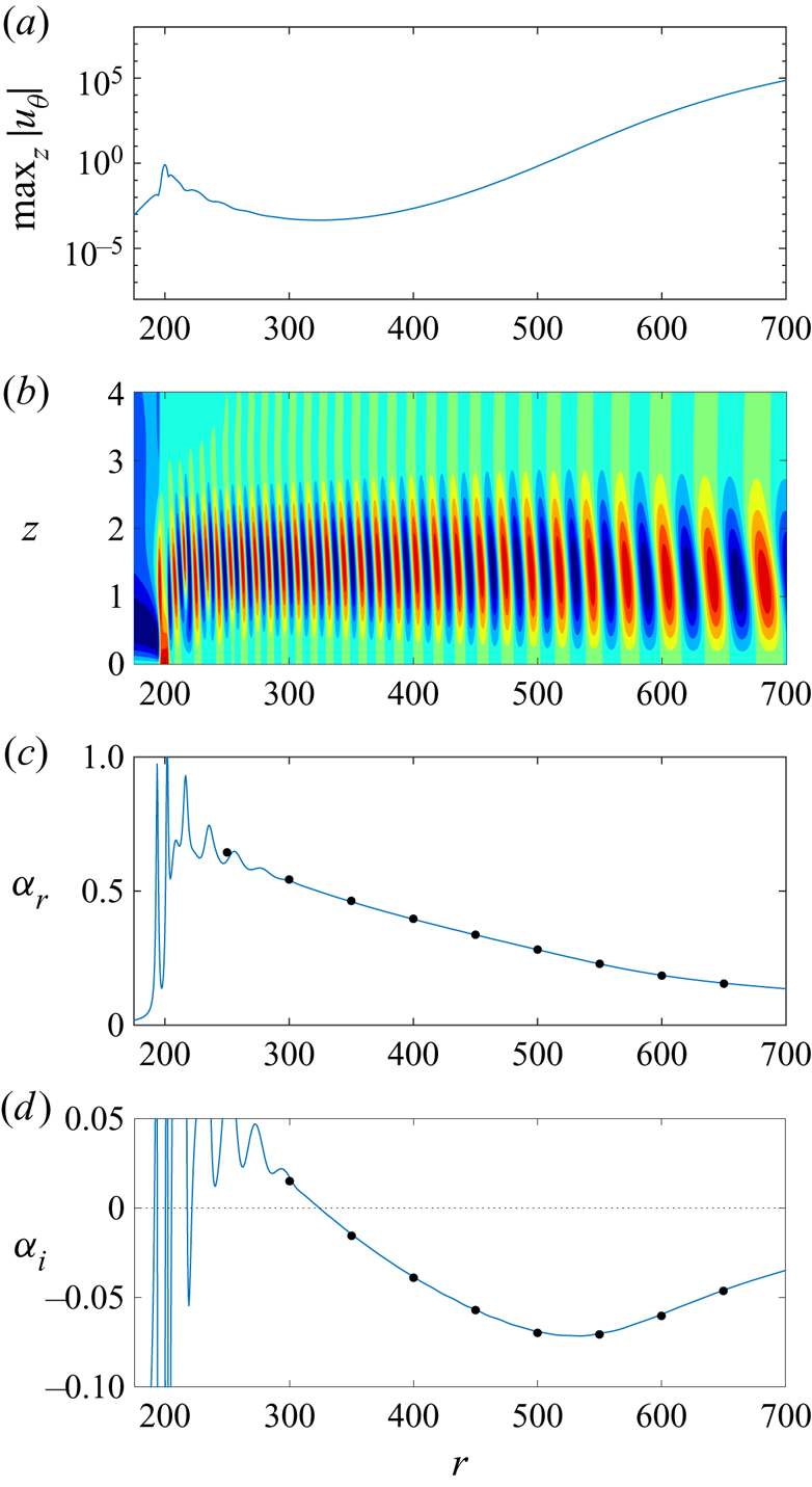
Figure 2 displays several characteristics associated with the linear disturbance established above. The maximum absolute value of the azimuthal velocity perturbation field,  $\max _z|u_{\theta }|$, is plotted in figure 2(a) as a function of
 $r$, while figure 2(b) depicts the corresponding contours of
 $u_{\theta }$ scaled on
 $\max _z|u_{\theta }|$ in the
 $(r,z)$-plane. The scaling was implemented here to assist visualisation of the disturbance development, which would otherwise be impossible due to the rapid spatial growth associated with this form of instability. Red and blue colours in figure 2(b) depict positive and negative valued contour levels, respectively. The radial location of the roughness in figures 2(a) and 2(b) is made evident by the respective small peak and red contours located about the radius
 $r=200$. Immediately downstream of the roughness the amplitude of the disturbance decreases. This behaviour is to be expected, as this particular cross-flow instability does not become linearly unstable until the critical radius
 $r_c\approx 323$. However, radially downstream of
 $r_c\approx 323$ the disturbance grows rapidly, and the cross-flow instability assumes the typical structure and develops near the disc surface.
Characteristics of the linear azimuthal velocity perturbation field  $u_{\theta }$ excited about
 $r_f=200$, for an azimuthal mode number
 $n=32$. (a) Plot of
 $\max _z|u_{\theta }|$ as a function of
 $r$. (b) Contours of
 $u_{\theta }/\max _z|u_{\theta }|$ in the
 $(r,z)$-plane. (c) Radial wavenumber
 $\alpha _r$. (d) Radial growth rate
 $\alpha _i$. The dot markers in (c,d) indicate those results obtained for fixed Reynolds numbers
 ${\textit {Re}}$ derived by applying the homogeneous flow approximation.

The spatial development of the linear perturbation  $\hat {\boldsymbol {q}}$ (recall (3.9)) may be decomposed as
 \begin{equation} \hat{\boldsymbol{q}}(r,z)= \check{\boldsymbol{q}}(r,z)\exp\left(\textrm{i} \int_{r_c}^{r}\alpha (r') \,\mathrm{d} r'\right), \end{equation}
where  $\check {\boldsymbol {q}}$ is a slowly varying shape function and
 $\alpha =\alpha _r+\textrm {i}\alpha _i$ represents the complex-valued radial wavenumber. The real and imaginary parts of
 $\alpha$ may be interpreted as the respective radial wavenumber and growth rate of the linear disturbance, and may be computed by considering the formula
 \begin{equation} \alpha ={-}\dfrac{\textrm{i}}{f}\dfrac{\partial f}{\partial r}, \end{equation}
where  $f$ is taken to be a measure of the disturbance amplitude at any given radial and wall-normal location. As before, the azimuthal velocity perturbation field
 $u_{\theta }$ was selected, with computations based on measurements about the wall-normal height
 $z=1.5$. (Note that the calculations for
 $\alpha$ were not noticeably affected by shifting the wall-normal
 $z$-location.)
The radial wavenumber  $\alpha _r$ and growth rate
 $\alpha _i$, associated with the above disturbance, are plotted in figures 2(c) and 2(d) and indicate that there is an initial transient phase before linearly unstable behaviour emerges about the critical radius
 $r_c\approx 323$. (Note that a negative valued
 $\alpha _i$ corresponds to radial growth and unstable behaviour.) The black dot markers in figures 2(c) and 2(d) depict the equivalent results obtained by solving the linear system of governing equations (4.2) with the homogeneous flow approximation, where the radial dependence of the undisturbed flow (2.6) is removed by fixing
 $r={\textit {Re}}$. To the accuracy of the illustration, the homogeneous flow computations about fixed radii are identical to the inhomogeneous flow solution, with results tabulated in table 1.
5.1.2. Adjoint perturbation
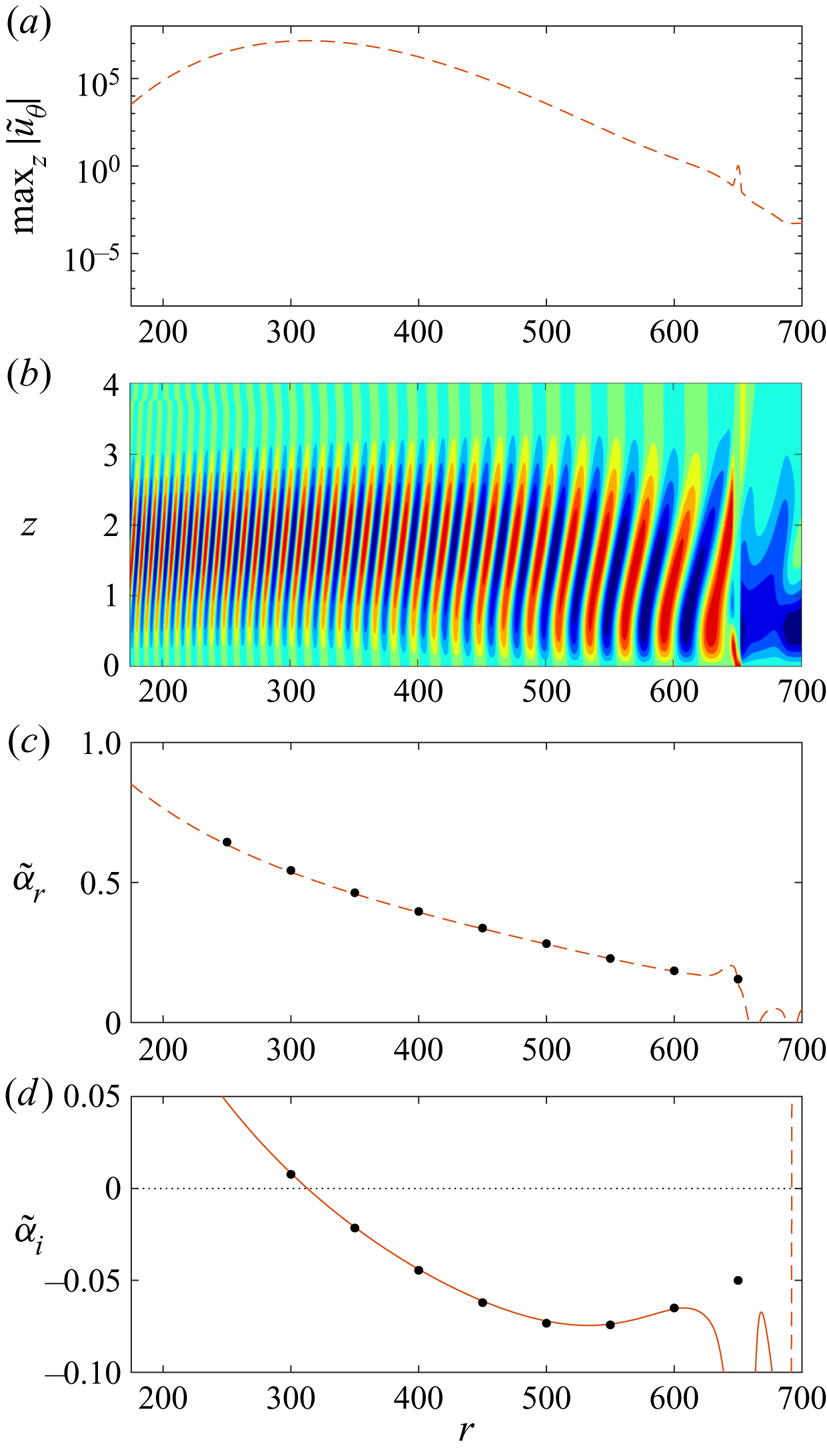
The corresponding adjoint perturbation field was generated by fixing the Gaussian shaped roughness (5.1) about the radius  $r_f=650$. Adjoint disturbances evolve in the spatially opposite sense to their linear counterparts and propagate upstream towards the inner radius. The dashed red line in figure 3(a) depicts the maximum absolute value of the adjoint perturbation field,
 $\max _z|\tilde {u}_{\theta }|$, while figure 3(b) displays the contours of
 $\tilde {u}_{\theta }$ scaled on
 $\max _z|\tilde {u}_{\theta }|$. The adjoint disturbance grows radially inwards, attaining a peak amplitude near the radial location that the linear cross-flow instability first becomes unstable. Further upstream, the magnitude of
 $\max _z|\tilde {u}_{\theta }|$ decreases, which corresponds to a decay in the adjoint perturbation field.
Characteristics of the adjoint azimuthal velocity perturbation field  $\tilde {u}_{\theta }$ excited about
 $r_f=650$, for an azimuthal mode number
 $n=32$. (a) Plot of
 $\max _z|\tilde {u}_{\theta }|$ as a function of
 $r$. (b) Contours of
 $\tilde {u}_{\theta }/\max _z|\tilde {u}_{\theta }|$ in the
 $(r,z)$-plane. (c) Radial wavenumber
 $\tilde {\alpha }_r$. (d) Radial growth rate
 $\tilde {\alpha }_i$. The dot markers in (c,d) indicate those results obtained for fixed Reynolds numbers
 ${\textit {Re}}$ derived by applying the homogeneous flow approximation.

Analogous to the linear perturbation, the spatial development of the adjoint perturbation  $\tilde {\hat {\boldsymbol {q}}}$ (recall (3.10)) may be decomposed as
 \begin{equation} \tilde{\hat{\boldsymbol{q}}}(r,z)= \tilde{\check{\boldsymbol{q}}}(r,z)\exp\left(-\textrm{i}\int_{\tilde{r}_c}^{r}\tilde{\alpha} (r') \,\mathrm{d} r'\right), \end{equation}
where  $\tilde {\check {\boldsymbol {q}}}$ is a slowly varying shape function and
 $\tilde {\alpha }=\tilde {\alpha }_r+\textrm {i}\tilde {\alpha }_i$ represents the complex-valued adjoint radial wavenumber. (Note a change in sign has been imposed on the adjoint radial wavenumber as the adjoint disturbance grows radially inwards.) The adjoint radial wavenumber
 $\tilde {\alpha }$ is determined via the formula
 \begin{equation} \tilde{\alpha} = \dfrac{\textrm{i}}{f}\dfrac{\partial f}{\partial r}, \end{equation}
with  $f$ taken as the adjoint azimuthal velocity perturbation field
 $\tilde {u}_{\theta }$, measured about the wall-normal height
 $z=1.5$.
Figures 3(c) and 3(d) depict the real and imaginary parts of  $\tilde {\alpha }$, with the adjoint growth rate
 $\tilde {\alpha }_i=0$ about the radius
 $\tilde {r}_c\approx 318$. (A negative valued
 $\tilde {\alpha }_i$ is matched to an adjoint perturbation growing radially inwards, while
 $\tilde {r}_c \neq r_c$ as a consequence of marginal differences between the linear and adjoint radial growth rates.) Black dot markers correspond to those solutions obtained by solving the equivalent adjoint system of governing equations (4.9) but with the application of the homogeneous flow approximation, i.e. the radius
 $r$ is held fixed by setting it equal to the Reynolds number
 ${\textit {Re}}$. Similar to the analysis of the linear perturbation, homogeneous flow calculations about fixed radii (tabulated in table 1) are indistinguishable from the inhomogeneous flow solutions. Moreover, the real parts of the linear and adjoint radial wavenumbers are identical:
 $\alpha _r=\tilde {\alpha }_r$. On the other hand, there are marginal differences in the corresponding imaginary parts:
 $\alpha _i\neq \tilde {\alpha }_i$. However, these small differences are counterbalanced by the normalisation (3.13).
5.1.3. Normalisation
Linear and adjoint disturbances were then normalised using (3.13), with the corresponding azimuthal velocity perturbation fields,  $\max _z|u_{\theta }|$ and
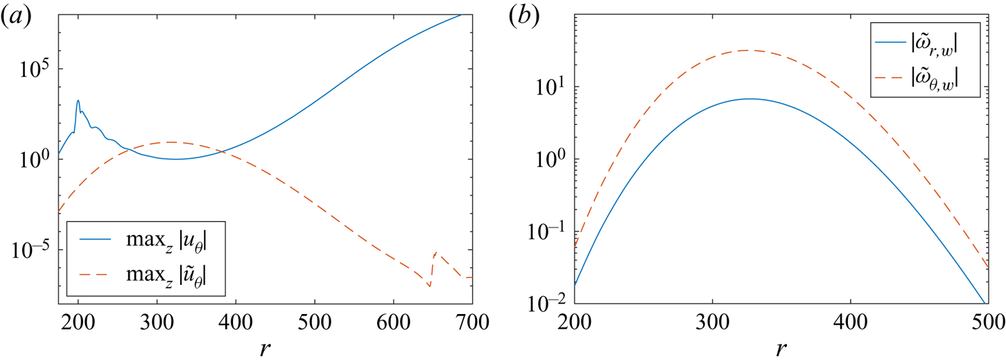
 $\max _z|\tilde {u}_{\theta }|$, plotted in figure 4(a). The line types and axes scales are the same as that given in figures 2(a) and 3(a), to help distinguish differences brought about by the normalisation. The linear solution is equal to unity about the radial location
 $r_c$ for the onset of the stationary cross-flow instability, which is a requirement of the normalisation (3.13). On the other hand, the adjoint solution is scaled downwards and develops at a significantly smaller amplitude than before the normalisation.
(a) Maximum absolute value of the linear and adjoint azimuthal velocity perturbation fields,  $\max _z|u_{\theta }|$ and
 $\max _z|\tilde {u}_{\theta }|$, normalised using (3.13). (b) Corresponding normalised absolute value of the adjoint vorticity perturbation fields,
 $|\tilde {\omega }_{r,w}|$ and
 $|\tilde {\omega }_{\theta ,w}|$. Solutions correspond to those parameter settings given in figures 2 and 3.

Figure 4(b) displays the normalised absolute value of the adjoint vorticity perturbation fields  $|\tilde {\omega }_{r,w}|$ (solid blue line) and
 $|\tilde {\omega }_{\theta ,w}|$ (dashed red line) that are required to compute the receptivity amplitude
 $A$ of the stationary cross-flow instability (recall (4.13)). The adjoint azimuthal vorticity perturbation field is almost an order of magnitude greater than the equivalent radial component. This would suggest that the azimuthal component of vorticity will have a greater influence on the receptivity of the rotating disc boundary layer to surface roughness. Furthermore, both adjoint perturbation fields achieve larger amplitudes about the radial location
 $r_c$ associated with the onset of the linear disturbance. Thus, we might expect receptivity to be enhanced by roughness elements located within this particular radial region.
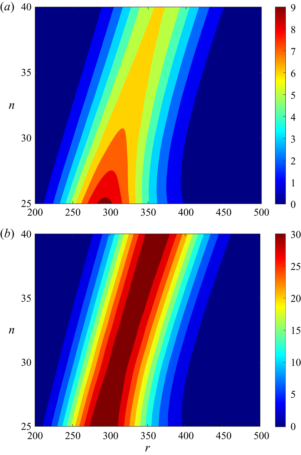
The above process was repeated for azimuthal mode numbers  $n\in [25,40]$ at unit step intervals. The decision to focus on this particular range of modes was made as a consequence of experimental investigations that typically observe cross-flow disturbances within this parameter range. Figure 5 depicts contours of
 $|\tilde {\omega }_{r,w}|$ and
 $|\tilde {\omega }_{\theta ,w}|$ in the
 $(r,n)$-plane. For azimuthal mode numbers
 $n\leqslant 32$, the two adjoint vorticity components attain a peak over the radial range
 $250\leqslant r\leqslant 350$. Beyond this annular region, both perturbation fields are significantly reduced. As
 $n$ increases, the radial location that the two adjoint vorticity terms achieve a maxima is shifted radially downstream. This particular observation coincides with a corresponding radial shift downstream in the onset of the stationary cross-flow instability that occurs as
 $n$ increases to larger values. Hence, for each azimuthal mode number
 $n$, receptivity will be most affected by surface roughness in the region that the stationary cross-flow instability first appears. This behaviour is consistent with that found in the flow over a swept wing. Radeztsky et al. (Reference Radeztsky, Reibert and Saric1999) undertook an experimental study on the flow over a swept wing with isolated roughness elements. Roughness centred about the location for neutral instability established the strongest receptivity, while roughness elements located further downstream had a negligible effect.
Contours in the  $(r,n)$-plane of (a)
 $|\tilde {\omega }_{r,w}|$; (b)
 $|\tilde {\omega }_{\theta ,w}|$.

5.2. Validation
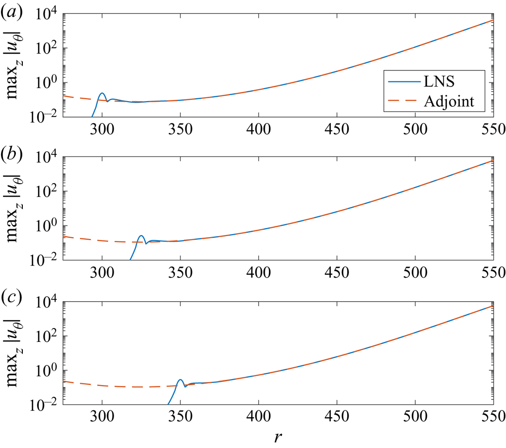
The adjoint scheme was validated by directly comparing adjoint predictions for the receptivity amplitude  $A$ against numerical solutions of the linear scheme (4.2). Linear disturbances were established by Gaussian shaped roughness elements (5.1) fixed about the radii
 $r_f=300$,
 $325$ and
 $350$. The solid blue lines in figure 6 depict the maximum absolute value of the azimuthal velocity perturbation field,
 $\max _z|u_{\theta }|$, established by these three roughness distributions.
Maximum absolute value of the azimuthal velocity perturbation field,  $\max _z|u_{\theta }|$, for the azimuthal mode number
 $n=32$. Stationary cross-flow disturbance excited by a Gaussian shaped roughness centred about (a)
 $r_f=300$; (b)
 $r_f=325$; (c)
 $r_f=350$. The LNS solution is given by the solid blue line, while the dashed red line depicts the adjoint prediction.

Coupling the receptivity formula (4.13) with the normalised adjoint vorticity perturbation fields  $\tilde {\omega }_{r,w}$ and
 $\tilde {\omega }_{\theta ,w}$, the amplitude
 $A$ of the disturbance established by the three Gaussian shaped roughnesses was instantaneously computed as
 $A=0.078$,
 $0.111$ and
 $0.106$, respectively. (Note that we only present the absolute value of the receptivity amplitude
 $A$ here.) The dashed red lines in figure 6 illustrate the adjoint predictions for
 $\max _z|u_{\theta }|$ that were obtained by scaling the normalised linear perturbation field (plotted in figure 4a) by the above adjoint prediction for the amplitude
 $A$. In all three instances, the linear and adjoint solutions are identical downstream of the roughness. Hence, the adjoint approach has correctly computed the amplitude
 $A$ of the stationary cross-flow instability excited by the three Gaussian shaped roughness distributions. Several further test cases were modelled, for different roughness locations and shapes. In each instance, the adjoint method correctly predicted the amplitude of the equivalent LNS generated disturbance.
Having successfully tested the adjoint method for predicting the amplitude  $A$ of the disturbance established by simple Gaussian shaped roughness elements, we extend the investigation to realistic surface distributions. As the adjoint formula (4.13) only requires the adjoint perturbation fields
 $\tilde {\omega }_{r,w}$ and
 $\tilde {\omega }_{\theta ,w}$ (given in figure 5) and the radial shape of the roughness
 $h(r)$ as inputs, the adjoint approach offers significant computational and time advantages over alternative receptivity strategies (i.e. LNS). Using (4.13), we undertake a rapid receptivity study of the rotating disc boundary layer to many thousands of randomly generated roughness realisations, of variable length and roughness settings.
5.3. Randomly distributed surface roughness
5.3.1. Model
Natural surface roughness is random and will be composed of several peaks and troughs of variable height, depth and wavelength. Mughal & Ashworth (Reference Mughal and Ashworth2013) undertook a receptivity investigation of stationary cross-flow vortices on a swept wing, whereby three-dimensional roughness distributions were modelled using a Fourier cosine series. A simplification was made in the subsequent adjoint based study by Thomas et al. (Reference Thomas, Mughal and Ashworth2017), who assumed the roughness distribution was periodic along the spanwise direction. A similar simplification was implemented here, where due to the natural periodicity of the disc, surface roughness was assumed to be periodic in the azimuthal direction. Two-dimensional roughness distributions were modelled as
 \begin{equation} h(r)=\sum_{j=N_{min}}^{N_{max}}a_j\cos\left(2{\rm \pi} \left(\frac{jr}{r_{\lambda}}+\phi_j\right)\right),\end{equation}
where  $N_{min}$ and
 $N_{max}$ specify long and short scale wavelength filters, and
 $r_{\lambda }$ denotes a radial wavelength. Parameters
 $a_j$ and
 $\phi _j$ represent randomly generated roughness amplitudes and phase shifts, respectively. Roughness distributions were then implemented on the radial interval
 $r_a \leqslant r \leqslant r_b$, where
 $r_a$ and
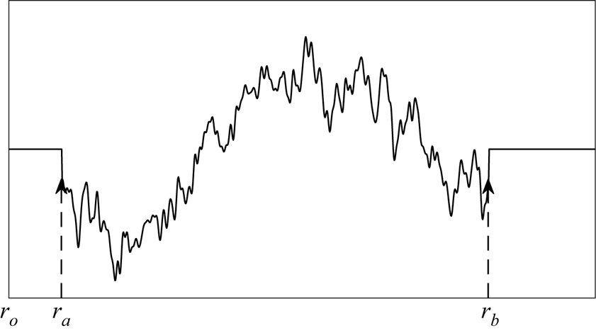
 $r_b$ specify the upstream and downstream boundaries of the surface roughness, respectively. Figure 7 displays a diagram of the roughness arrangement, including labels for the radial positions
 $r_o$,
 $r_a$ and
 $r_b$. (Note that in the subsequent analysis, the downstream boundary of the roughness distribution
 $r_b\leqslant r_{\lambda }+r_a$.)
Diagram of the roughness model.

Each randomly generated amplitude  $a_j$ was then scaled by the factor
 \begin{equation} \left(\dfrac{r_{\lambda}}{2{\rm \pi} j}\right)^{k} \end{equation}
for a power law coefficient  $k$. An identical modelling approach was implemented by Raposo et al. (Reference Raposo, Mughal and Ashworth2018) in their acoustic receptivity study of TS waves in the presence of surface roughness. This particular model for roughness was utilised here as it is well known that the power spectral density (PSD) for natural surface roughness follows a power law of the form (5.5) (Van Deusen Reference Van Deusen1967; Sayles & Thomas Reference Sayles and Thomas1978; Jacobs, Junge & Pastewka Reference Jacobs, Junge and Pastewka2017). For instance, it was shown by Mughal & Ashworth (Reference Mughal and Ashworth2013) that the energy in the PSD of a painted panel or unpainted aluminium plate was primarily found in the longer wavelengths. Furthermore, Van Deusen (Reference Van Deusen1967) noted that the PSD decreased with the square of the angular frequency for many natural and artificial surfaces, while Raposo et al. (Reference Raposo, Mughal and Ashworth2018) set the coefficient
 $k=1$ in their receptivity investigation to ensure the PSD decayed at the rate found by Van Deusen.
Finally, all roughness distributions were scaled on the r.m.s., which is defined as
 \begin{equation} h_{{rms}}=\sqrt{\dfrac{1}{r_b-r_a}\int_{r_a}^{r_b}h^2 \,\mathrm{d} r}. \end{equation}
For instance, setting  $h_{{rms}}=10^{-3}$ corresponds to a surface roughness with a r.m.s. equal to
 $0.1\,\%$ of the boundary layer thickness
 $\delta$.
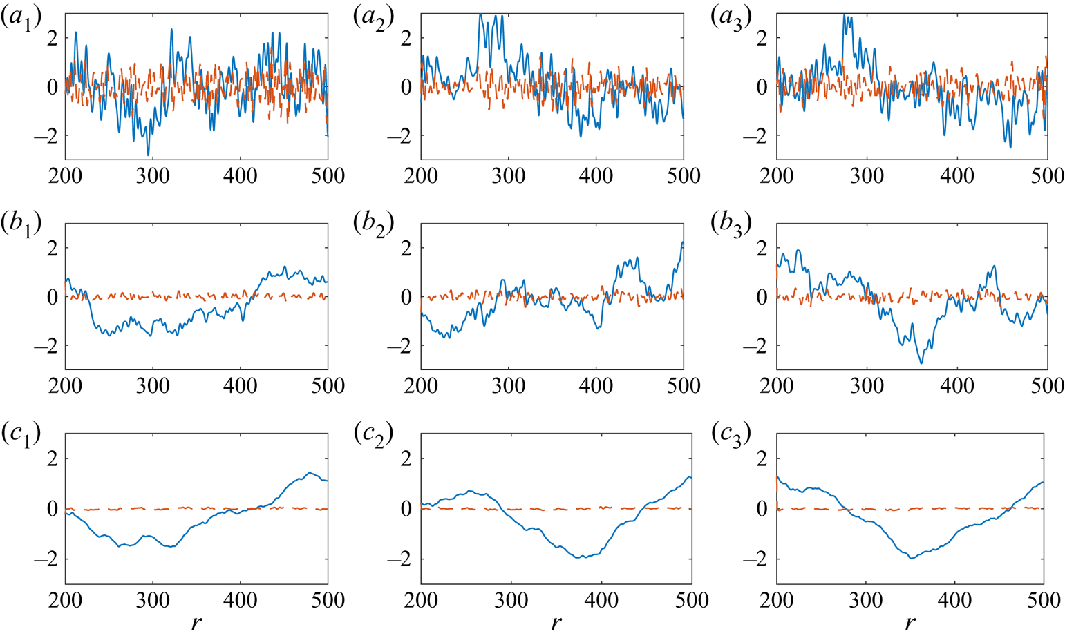
Figure 8 depicts several randomly generated roughness distributions (solid blue lines), along with their respective gradients  $\textrm {d}h/\textrm {d}r$ (dashed red) in the instance the roughness parameter
 $h_{{rms}}=1$. The long and short scale wavelength filters are set to the respective values
 $N_{min}=1$ and
 $N_{max}=100$, while each roughness is fixed about the radial interval
 $200\leqslant r\leqslant 600$ and
 $r_{\lambda }=400$. The power law coefficient
 $k$ increases from
 $k=0.5$ in figure 8(a) to
 $k=1.5$ in figure 8(c), at
 $0.5$ step intervals. The illustration clearly shows that each roughness realisation is distinct and encompasses a variety of wavelengths. Furthermore, the effect of the power law coefficient
 $k$ on the form of the roughness is demonstrated. For small
 $k$, shorter wavelengths are significant that establish many peaks and troughs with relatively large gradients. However, as the coefficient
 $k$ increases, shorter wavelengths have a limited influence on the structure of the roughness, resulting in fewer sharp variations and significantly smaller gradients.
Examples of surface roughness for  $N_{{min}}=1$,
 $N_{{max}}=100$,
 $h_{{rms}}=1$ and (a
 $_{\star }$)
 $k=0.5$; (b
 $_{\star }$)
 $k=1$; (c
 $_{\star }$)
 $k=1.5$. The solid blue and dashed red lines depict roughness distributions
 $h$ and their corresponding gradients
 $\textrm {d}h/\textrm {d}r$.

Averaging over many thousands of roughness realisations, it was determined that the mean of the absolute value of the surface gradient,  $|\textrm {d}h/\textrm {d}r|$, was approximately
 $0.4$ when
 $k=0.5$, but reduces as
 $k$ increases;
 $|\textrm {d}h/\textrm {d}r|\approx 0.1$ and
 $0.05$ for
 $k=1$ and
 $k=1.5$, respectively. These trends are then scaled linearly with the r.m.s. of the roughness. In the subsequent analysis we assume that any significant spikes or troughs in the surface roughness are not sufficient to bring about boundary layer separation or the nonlinear stages of laminar–turbulent transition.
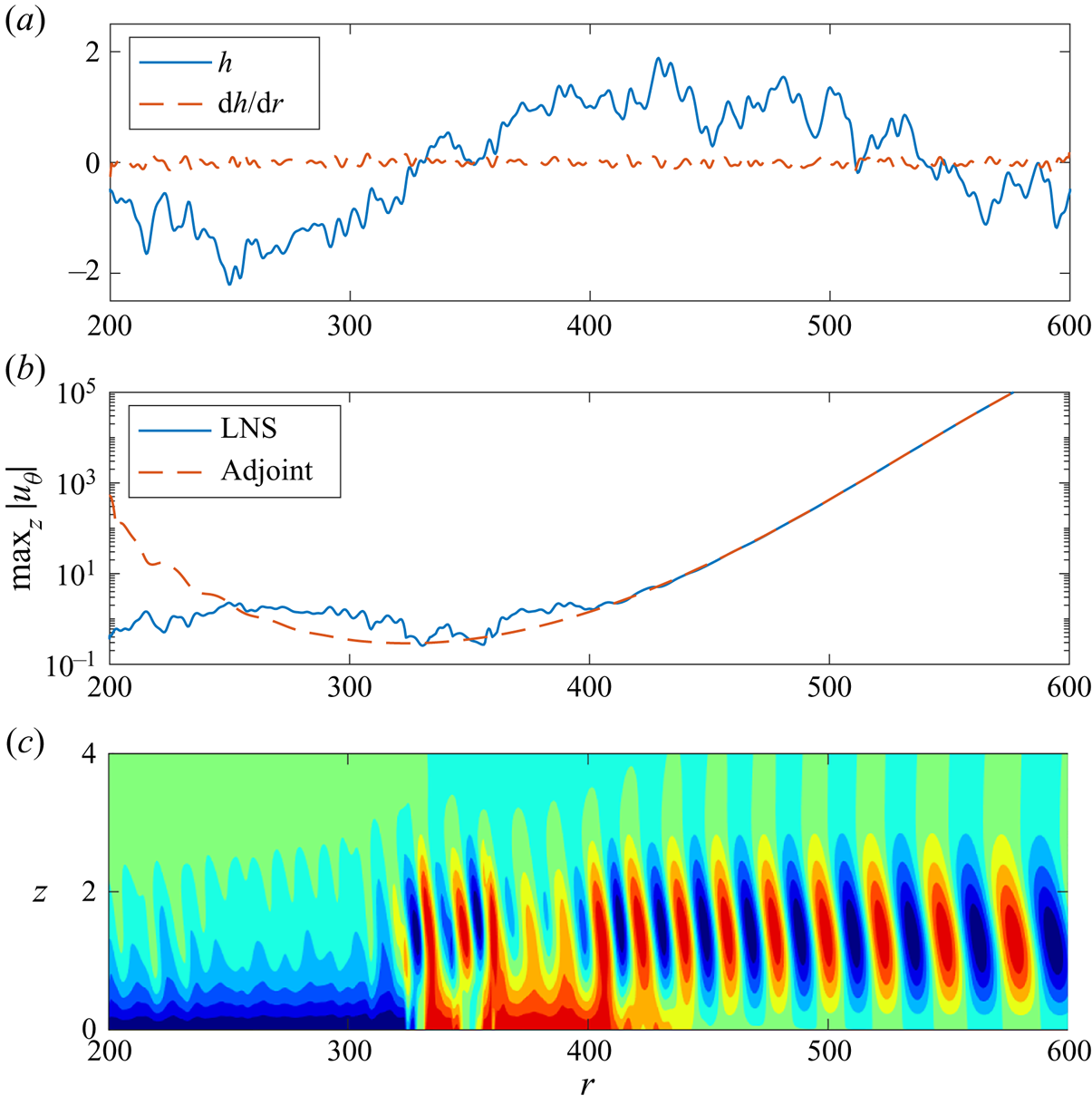
An additional roughness realisation is plotted in figure 9(a) that is established using those parameter settings given in figure 8(b). The response of the azimuthal velocity perturbation field  $u_{\theta }$, to this particular roughness, is then shown in figure 9(b,c). The maximum absolute value of the azimuthal velocity perturbation field,
 $\max _z|u_{\theta }|$, determined via the LNS formulation (4.2) is given by the solid blue line in figure 9(b), while the equivalent adjoint prediction is given by the dashed red line. (Recall that the adjoint formula (4.13) only requires the normalised adjoint vorticity fields
 $\omega _{r,w}$ and
 $\omega _{\theta ,w}$, and the roughness shape
 $h$, as inputs.) The amplitude
 $A$ of the disturbance established by the given roughness was determined using the adjoint formula (4.13) as
 $A=0.29$. As with the simpler Gaussian shaped roughness distributions, the LNS solution and adjoint prediction are indistinguishable. Thus, the adjoint approach has again correctly determined the amplitude
 $A$ of the disturbance.
(a) Randomly generated roughness distribution  $h$ and gradient
 $\textrm {d}h/\textrm {d}r$. (b) Maximum absolute value of the azimuthal velocity perturbation field,
 $\max _z|u_{\theta }|$. The LNS solution is given by the solid blue line, while the dashed red line depicts the adjoint prediction. (c) Contours of
 $u_{\theta }$, scaled on
 $\max _z|u_{\theta }|$, in the
 $(r,z)$-plane.

The depiction of  $\max _z|u_{\theta }|$ in figure 9(b) and the contours of
 $u_{\theta }$ in figure 9(c) indicate that the disturbance achieves magnitudes greater than the height of the roughness about the radius
 $r=400$. Beyond this radial location the disturbance grows rapidly, and the response of the linear perturbation is not affected by roughness elements located further outboard. Hence, receptivity is greatest in the radial region that the stationary cross-flow instability first becomes linearly unstable.
5.3.2. Mean receptivity
For the remainder of this investigation, the long wavelength filter  $N_{min}=1$ and the wavelength parameter
 $r_{\lambda }=400$. Additionally, the upstream boundary of the roughness distribution was fixed about
 $r_a=200$, which is sufficiently far upstream of the radial region that receptivity is expected to be the most significant. The downstream boundary
 $r_b$ of the roughness distribution and the short wavelength filter
 $N_{max}$ were then varied to determine the effects, if any, on the receptivity process. Additionally, several values of the power law coefficient
 $k$ were modelled.
There are two major objectives of the following analysis.
(i) Determine those roughness characteristics that are most significant in the receptivity process, and establish the largest disturbance amplitudes
 $A$.
(ii) For a disc with a known roughness r.m.s., compute the mean disturbance amplitudes and determine the radial region that disturbances achieve sufficiently large magnitudes to invalidate the linear stability assumptions. Moreover, these calculations will be used as initial inputs in a future fully nonlinear stability study.

A Monte-Carlo uncertainty quantification analysis was undertaken, whereby several thousand roughness distributions were randomly generated and receptivity amplitudes  $A$ computed. Mean amplitudes
 $\bar {A}$ were then determined via the formula
 \begin{equation} \bar{A}=\sum_s A/s, \end{equation}
for  $s$ roughness realisations. (Calculations were again based on the absolute value of
 $A$.) Figure 10(a) displays mean amplitudes
 $\bar {A}$ as a function of the number of roughness realisations
 $s$, for four downstream boundaries
 $r_b$. The azimuthal mode number
 $n=32$ and the low wavelength filter
 $N_{max}=100$, while the roughness parameter
 $h_{{rms}}$ and power law coefficient
 $k$ were both set to unity. A log scaling is used along the horizontal
 $s$-axis to illustrate the variation in
 $\bar {A}$ as
 $s$ increases. In all instances modelled, the size of
 $\bar {A}$ converges towards a fixed constant after approximately
 $1000$ roughness iterations. Further iterations were not found to bring about any significant changes in the mean amplitude. Although a different mean amplitude was realised for each
 $r_b$ considered, results indicate that variations in
 $\bar {A}$ diminish as
 $r_b$ increases. Thus, surface roughness located sufficiently far outboard has a negligible effect on the mean amplitude of the stationary cross-flow instability.
(a) Mean amplitude  $\bar {A}$ against the number of roughness realisations
 $s$. (b) Probability density functions. The azimuthal mode number
 $n=32$ and roughness parameters
 $N_{{max}}=100$,
 $h_{{rms}}=1$,
 $k=1$ and variable
 $r_b$.

Probability density functions (p.d.f.s) are plotted in figure 10(b), which were generated using the routines available in MATLAB. Each p.d.f. was constructed using  $s=10^4$ roughness realisations and the absolute value of the receptivity amplitude
 $A$. Solutions indicate that a greater variance in the amplitude
 $A$ is achieved as the length of the roughness distribution increases. Moreover, the illustration shows that receptivity can vary significantly from one realisation to the next. It is hypothesised that the larger amplitudes are associated with roughness distributions that encompass significant isolated peaks (and troughs) in the radial region that receptivity is most enhanced, i.e. where the cross-flow vortex first becomes linearly unstable.
Mean amplitudes  $\bar {A}$ are plotted as a function of the low wavelength filter
 $N_{max}$ (for
 $r_b=600$) in figure 11(a) and the downstream boundary
 $r_b$ of the roughness (for
 $N_{max}=100$) in figure 11(b). Solutions again correspond to the stationary cross-flow instability established for the azimuthal mode number
 $n=32$, while roughness parameters
 $h_{{rms}}=1$ and
 $k\in [0.5,1.5]$. Moreover, computations are based on
 $s=10^4$ roughness realisations, which was more than sufficient for
 $\bar {A}$ to achieve a converged state in all cases modelled. The size of the mean amplitude
 $\bar {A}$ increases sharply in figure 11(a) when
 $N_{max}$ exceeds 20. This particular observation coincides with the shortest roughness scale matching the wavelength of the cross-flow instability. The radial wavenumber
 $\alpha _r$ of the stationary cross-flow instability is within the range
 $0.25\leqslant \alpha _r\leqslant 0.5$ (recall figure 2c), while the wavenumber associated with the shortest roughness scale in (5.4) is given as
 $2{\rm \pi} N_{max}/r_{\lambda }\approx 0.31$ for
 $N_{max}=20$. Similar observations were observed by Thomas et al. (Reference Thomas, Mughal and Ashworth2017) in their receptivity study of cross-flow vortices over a swept wing. With the exception of the case
 $k=0.5$ (solid blue line), mean amplitudes
 $\bar {A}$ approach a fixed constant for
 $N_{max}\approx 40$, which corresponds to a roughness length scale that is approximately half of the wavelength of the cross-flow instability. Hence, shorter roughness scales have a negligible effect on the receptivity process, which is to be expected given the power law scale factor (5.5). In the instance the power law coefficient
 $k=0.5$,
 $\bar {A}$ is observed to decrease for
 $N_{max}>40$. However, if results were extended to larger valued
 $N_{max}$, than that plotted in figure 11(a), results would eventually converge towards a fixed value as the shorter roughness scales would become insignificant. Finally, as
 $k$ increases, the size of the mean amplitude
 $\bar {A}$ decreases. Indeed, there is an order of magnitude difference in
 $\bar {A}$ between the smallest and largest valued
 $k$ modelled. The significance of the short roughness scales of commensurate size to the wavelength of the cross-flow instability, diminish for larger valued
 $k$.
Mean amplitude  $\bar {A}$ as a function of (a)
 $N_{max}$ for
 $r_b=600$ and (b)
 $r_b$ for
 $N_{max}=100$. Computations are based on
 $s=10^4$ roughness iterations for
 $n=32$, and roughness parameters
 $h_{{rms}}=1$ and variable
 $k$.

Results plotted in figure 11(b) indicate that the mean amplitude  $\bar {A}$ increases rapidly for radii
 $r_b>250$, and in most instances asymptotes towards a fixed constant for
 $r_b>400$. (There is a noticeable exception for cases
 $k>1$, where
 $\bar {A}$ attains a maximum value near
 $r_b\approx 330$ and then decreases towards a fixed constant for larger valued
 $r_b$. This behaviour can again be attributed to the diminished effect of the short roughness scales that occurs for larger valued
 $k$.) These observations are consistent with our earlier predictions that receptivity is most affected by roughness distributions located about the radial region that the disturbance first becomes linearly unstable and where the adjoint vorticity terms were most significant (recall figures 4(b) and 5).
The above analysis was extended to azimuthal mode numbers  $n\in [25,40]$, for roughness parameter settings
 $N_{max}=100$,
 $r_b=600$ and
 $h_{{rms}}=1$. These particular settings were chosen as receptivity calculations were unchanged by further increases in the short wavelength filter
 $N_{max}$ or the downstream boundary
 $r_b$ of the roughness. Figure 12 displays the mean amplitude
 $\bar {A}$ and corresponding standard deviations
 $\sigma$ as functions of
 $n$, for five values of the power law coefficient
 $k$. Calculations are again based on
 $s=10^4$ roughness realisations. For each
 $k$ considered, the standard deviation
 $\sigma$ is approximately half of the corresponding mean amplitude
 $\bar {A}$. Thus, there is a significant variation in the initial amplitude of the stationary cross-flow instability. Additionally, there is a small increase in
 $\bar {A}$ as the azimuthal mode number
 $n$ increases. However, this does not necessarily imply that these larger valued
 $n$ modes will play a greater role in the laminar–turbulent transition process, as smaller valued
 $n$ modes become unstable earlier. The cross-flow mode that is ultimately responsible for bringing about the latter stages of convective driven transition is governed by the amplitude
 $A$, the radial growth rate
 $\alpha _i$ and the size of the roughness that is characterised in this investigation by the parameter
 $h_{{rms}}$.
(a) Mean amplitude  $\bar {A}$ and (b) standard deviation
 $\sigma$ as a function of the azimuthal mode number
 $n$ and variable
 $k$. Computations are based on
 $s=10^4$ roughness iterations, and roughness parameters
 $h_{{rms}}=1$,
 $N_{max}=100$ and
 $r_b=600$. Line types are the same as those given in figure 11.

5.3.3. Predicting the onset of nonlinear behaviour and other processes
Mean amplitudes  $\bar {A}$ are coupled to the radial growth of the normalised azimuthal velocity perturbation field
 $u_{\theta }$ (as plotted in figure 4(a) for
 $n=32$) to predict the radial location that we might expect the linear stability assumptions to no longer be appropriate, and where nonlinear effects and other transition processes to have emerged. Since the analysis is linear, scaling the surface roughness on the parameter
 $h_{{rms}}$ equates to an equivalent scaling on the disturbance amplitude. Thus, fixing
 $h_{{rms}}=10^{-3}$ corresponds to setting the mean amplitude of the disturbance to
 $10^{-3}\bar {A}$, with
 $\bar {A}$ as given in figure 12. Furthermore, we assume that the linear stability assumptions are no longer appropriate once
 $\max _z|u_{\theta }|=10^{-1}$. This particular assumption was based on earlier observations within the literature. For instance, Balachandar, Streett & Malik (Reference Balachandar, Streett and Malik1992) reported that the primary instability has to attain a threshold value of
 $9\,\%$ of the undisturbed flow (2.6) in order for secondary instabilities to grow. Hence,
 $r_{u_{\theta }=0.1}$ denotes the radial location used here to distinguish between the linear and nonlinear stages of convectively forced laminar–turbulent transition. (In experiments, the threshold between linear and nonlinear effects may arise at smaller disturbance amplitudes than that implemented here. Moreover, travelling waves, the absolutely unstable mechanism or secondary instabilities may develop, and establish nonlinear behaviour and the onset of laminar–turbulent transition at earlier radii than that presented in the subsequent analysis. Thus, the radial location
 $r_{u_{\theta }=0.1}$ should only be viewed as an upper bound for when we might expect disturbance development to be no longer governed by linear stability theory.)
Figure 13 displays the maximum absolute value of the azimuthal velocity perturbation field,  $\max _z|u_{\theta }|$, as a function of the radius
 $r$ for the azimuthal mode number
 $n=32$. Solution curves were obtained by scaling the normalised solution depicted in figure 4(a), by the adjoint predictions for the mean amplitude
 $\bar {A}$ presented in figure 12, with
 $k$ set to unity. The horizontal dotted line indicates when
 $\max _z|u_{\theta }|=10^{-1}$. (Computations based on other
 $k$ values brought about a small change in the radial interval that
 $\max _z|u_{\theta }|=10^{-1}$ was realised.) The r.m.s. of the roughness decreases by an order of ten monotonically down figure 13, with
 $h_{{rms}}=10^{-2}$ and
 $10^{-4}$ in figures 13(a) and 13(c), respectively. Solid blue line-types depict results based on the mean amplitude
 $\bar {A}$, while the remaining two line-types give an indication of the spread of solutions, with the disturbance amplitude set to
 $\bar {A}\pm \sigma$. Results indicate that
 $\max _z|u_{\theta }|=10^{-1}$ is realised about the successive radial intervals
 $r\in [418,450]$,
 $[460,485]$ and
 $[495,520]$, for the three respective
 $h_{{rms}}$ values modelled. This was extended to
 $r\in [528,550]$ and
 $[560,583]$ for
 $h_{{rms}}=10^{-5}$ and
 $10^{-6}$, respectively. Hence, for a fixed
 $h_{{rms}}$, there is a short annular region in which we might expect the stationary cross-flow vortex, established by surface roughness, to achieve amplitudes sufficient to invalidate the linear stability assumptions and bring about nonlinear effects. Furthermore, results clearly demonstrate that a smooth disc will delay the onset of convective induced transition to larger radii, which may allow the absolutely unstable mechanism to develop and play a role in the laminar–turbulent transition process.
Maximum absolute value of the azimuthal velocity perturbation field,  $\max _z|u_{\theta }|$, as a function of the radius
 $r$ for
 $n=32$ and (a)
 $h_{{rms}}=10^{-2}$; (b)
 $h_{{rms}}=10^{-3}$; (c)
 $h_{{rms}}=10^{-4}$. Calculations are based on those roughness parameters given in figure 12 when
 $k=1$. The horizontal dotted line corresponds to
 $\max _z|u_{\theta }|=10^{-1}$.

The radial location  $r_{u_{\theta }=0.1}$ is plotted in figure 14 as a function of
 $h_{{rms}}$. Calculations are again based on the adjoint predictions presented in figure 12 for
 $n=32$. The first illustration, figure 14(a), gives an indication of the spread of
 $r_{u_{\theta }=0.1}$ for the case where the power law coefficient
 $k=1$. The second plot, figure 14(b), depicts the effect of varying the power law coefficient
 $k$. As expected, results show that the radial location
 $r_{u_{\theta }=0.1}$ emerges further downstream as
 $h_{{rms}}$ decreases. Furthermore, for
 $h_{{rms}}\leqslant 10^{-2}$, the radius
 $r_{u_{\theta }=0.1}$ is approximated by the formula
 \begin{equation} r_{u_{\theta}=0.1}=c-d\log_{10}h_{{rms}} \end{equation}
for positive valued constants  $c$ and
 $d$ that are dependent on
 $k$. (Similar depictions of
 $r_{u_{\theta }=0.1}$ were realised for other stationary cross-flow disturbances with different azimuthal mode numbers.) Assuming that experimental roughness characteristics are known and that the
 $n=32$ cross-flow mode is responsible for bringing about convective driven transition, figure 14 and this particular logarithmic relationship may be used to predict the radial range when transition in the rotating disc boundary layer is likely to occur, or at least when nonlinear effects and other processes must be accounted for. Finally, results imply that
 $r_{u_{\theta }=0.1}$ occurs further downstream for larger valued
 $k$, which is to be expected given our earlier observations: mean amplitudes
 $\bar {A}$ decrease as
 $k$ increases.
The radius  $r$ that the maximum absolute value of the azimuthal velocity perturbation field,
 $\max _z|u_{\theta }|=10^{-1}$, for
 $n=32$ and those roughness parameters given in figure 12. (a) Calculations are based on the mean amplitude
 $\bar {A}$ and standard deviation
 $\sigma$ for
 $k=1$. (b) Calculations are based on
 $\bar {A}$ and variable
 $k$.

The maximum absolute value of the azimuthal velocity perturbation field,  $\max _z|u_{\theta }|$, is plotted in figure 15 for several azimuthal mode numbers
 $n$. Computations are again based on the mean calculations presented in figure 12 for
 $k=1$, while the roughness parameter
 $h_{{rms}}$ is as indicated in the caption. The horizontal dotted line again specifies when
 $\max _z|u_{\theta }|=10^{-1}$. Solutions plotted in figure 15(a) indicate that the
 $n=26$ cross-flow mode (solid blue line) attains this threshold value about
 $r\approx 400$ when
 $h_{{rms}}=10^{-2}$, which is radially inboard of the locations that the other modes achieve this particular amplitude. Thus, the
 $n=26$ mode will be responsible for engineering the early stages of transition in this instance. As
 $h_{{rms}}$ decreases, the stationary cross-flow mode
 $n$ that first achieves the amplitude
 $\max _z|u_{\theta }|=10^{-1}$, increases. For
 $h_{{rms}}=10^{-3}$ and
 $10^{-4}$, cross-flow modes
 $n=28$ (dashed red) and
 $30$ (chain yellow) are the first to attain the linear-nonlinear threshold amplitude about the respective radial positions
 $r\approx 450$ and
 $500$.
Maximum absolute value of the azimuthal velocity perturbation field,  $\max _z|u_{\theta }|$, as a function of the radius
 $r$ for variable azimuthal mode numbers
 $n$ and (a)
 $h_{{rms}}=10^{-2}$; (b)
 $h_{{rms}}=10^{-3}$; (c)
 $h_{{rms}}=10^{-4}$. Mean amplitudes
 $\bar {A}$ are based on those roughness parameter settings given in figure 12 when
 $k=1$. The horizontal dotted line corresponds to
 $\max _z|u_{\theta }|=10^{-1}$.

Contours of the radius  $r_{u_{\theta }=0.1}$ are plotted in figure 16 in the
 $(n,h_{{rms}})$-plane, for those roughness settings given in figure 12 and
 $k=1$. Blue contour levels correspond to radii
 $r\sim 400$, while red contours are matched to
 $r\sim 600$. The illustration further supports our above comments that azimuthal mode numbers on the interval
 $25\leqslant n\leqslant 30$ will most likely bring about nonlinear effects when the roughness parameter
 $h_{{rms}}\geqslant 10^{-4}$. However, for smaller valued
 $h_{{rms}}$, larger valued azimuthal mode numbers (such as
 $n=32$) grow at a faster rate and attain amplitudes
 $\max _z|u_{\theta }|=10^{-1}$ earlier. Hence, these particular stationary cross-flow instabilities will play a greater role in the early stages of laminar–turbulent transition on a clean rotating disc.
Contours of the radius  $r_{u_{\theta }=0.1}$ in the
 $(n,h_{{rms}})$-plane that the maximum absolute value of the azimuthal velocity perturbation field,
 $\max _z|u_{\theta }|=10^{-1}$. Mean amplitudes
 $\bar {A}$ are based on those roughness parameter settings given in figure 12 when
 $k=1$.

6. Conclusions
The receptivity of the rotating disc boundary layer to surface roughness was investigated using adjoint methods. The ALNS equations in cylindrical coordinates were derived and receptivity characteristics were computed using a fully equivalent velocity–vorticity formulation (that is based on the numerical scheme developed by Davies & Carpenter Reference Davies and Carpenter2001). Stationary cross-flow vortices were excited by surface roughness that was modelled using a two-dimensional Fourier cosine series (5.4) and implemented via a linearisation of the no-slip condition. Each roughness distribution was scaled on its respective r.m.s. and composed of many roughness length scales (both long and short) that establish distinct surface distributions. Randomness was modelled by assigning each roughness length scale a randomly generated amplitude and phase shift. Furthermore, roughness amplitudes were scaled using a power law (5.5) that was characterised by a coefficient  $k$, that ensures the energy of the PSD was primarily found in the longer roughness wavelengths (Van Deusen Reference Van Deusen1967). A receptivity formula, based on adjoint perturbation fields, was formulated and used to predict the receptivity or initial amplitude of the stationary cross-flow instability established by surface roughness. The amplitude of the disturbance, generated by surface roughness, is then instantaneously determined by a simple integration of known quantities; normalised adjoint vorticity fields and the roughness shape. Thus, the adjoint approach for receptivity offers huge computational and time advantages over slower LNS based receptivity strategies.
Adjoint perturbation fields, required to predict receptivity, were considerably larger about the radial range that the stationary cross-flow instability first appears. Indeed, receptivity was significantly enhanced by surface roughness located about this annular region. This behaviour is consistent with observations on a swept wing (Radeztsky et al. Reference Radeztsky, Reibert and Saric1999), where the receptivity of stationary cross-flow vortices is strongest near the leading edge.
A Monte-Carlo type uncertainty quantification analysis was undertaken, whereby many thousands of roughness distributions were randomly generated and disturbance amplitudes determined. Receptivity characteristics were averaged over all roughness realisations to compute the expected mean amplitudes and spread. Disturbance amplitudes were noticeably enhanced by roughness distributions that include short roughness scales equivalent to the wavelength of the stationary cross-flow instability. Very short roughness scales, approximately half a cross-flow vortex wavelength and less, were found to have a negligible effect on the receptivity process, which were further diminished as the power law coefficient  $k$ increases. Furthermore, mean amplitudes increased significantly for roughness elements fixed about the radial interval
 $200 \leqslant r \leqslant 400$, while receptivity was less affected by surface roughness located further outboard.
The onset of the nonlinear stage in the laminar–turbulent transition process was estimated by coupling the adjoint predictions for the mean amplitude with the radial growth of the stationary cross-flow instability. The r.m.s. of the roughness was varied to determine the effects on transition brought about by this convectively unstable disturbance. It was assumed that the linear stability assumptions were invalid and nonlinear effects emerged about the radial location that the azimuthal velocity perturbation field attained a magnitude of order  $10^{-1}$. Results suggest that for relatively large roughness r.m.s. values (greater than
 $10^{-4}$), stationary cross-flow modes
 $n\leqslant 30$ will achieve the linear–nonlinear threshold first, and thus, will be responsible for the appearance of nonlinear behaviour and engineering transition to turbulence. However, for smaller r.m.s. values that might be more representative of a clean rotating disc, marginally larger cross-flow modes,
 $n\geqslant 32$, were first to attain the threshold amplitude. Hence, these modes are expected to be significant in bringing about the latter stages of transition on a clean disc, which is consistent with many experimental and numerical observations.
The current investigation focuses on the development of stationary cross-flow disturbances in the infinite rotating disc boundary layer, which are assumed here to be responsible for the early stages of laminar–turbulent transition. The growth of travelling cross-flow waves established by acoustics or free-stream vortex structures, and mechanisms linked to local absolute instability (Lingwood Reference Lingwood1995), linear globally unstable disturbances (Thomas & Davies Reference Thomas and Davies2018) and disc edge effects (Healey Reference Healey2010; Imayama et al. Reference Imayama, Alfredsson and Lingwood2013; Pier Reference Pier2013; Appelquist et al. Reference Appelquist, Schlatter, Alfredsson and Lingwood2015, Reference Appelquist, Schlatter, Alfredsson and Lingwood2016) were ignored. For very small roughness r.m.s. values, the absolute route to turbulence may transpire (Imayama et al. Reference Imayama, Alfredsson and Lingwood2016) as the convectively growing cross-flow instabilities may not achieve sufficiently large amplitudes until further downstream. Additionally, the roughness model imposed in this study was assumed to be periodic in the azimuthal direction. In real experiments, roughness will be fully three dimensional and may be localised in both the radial and azimuthal directions. Thus, for future receptivity studies, it will be necessary to extend the simplified two-dimensional model (5.4) to three dimensions, and determine the effect on the receptivity process and disturbance amplitudes. Hence, to ascertain a greater understanding of the transition process on a rotating disc, we suggest that the mean disturbance amplitudes computed herein and from a fully three-dimensional roughness study be used as initial conditions in a fully global nonlinear instability investigation. The radial region that nonlinear effects can be expected to ensue can then be determined more precisely (as opposed to the estimates made above). Furthermore, by combining real profile measurements of a disc surface (made using a profilometer) with the adjoint receptivity formulation, it may be possible to specify the exact PSDs in the roughness model (5.4) and, hence, compute the expected mean disturbance amplitudes for experimental studies on the rotating disc.
Acknowledgements
We are grateful to the referees for several suggestions which have led to a much improved paper.
Declaration of interests
The authors report no conflict of interest.