2.1. Set-up

We have adapted the set-up described in Dollet (Reference Dollet2010). The foam flows in a Hele-Shaw cell, made of two horizontal glass plates of length 170 cm and width 32 cm, separated by a gap $h=2~\text{mm}$ thin enough that the foam is confined as a bubble monolayer (figure 1 a). Two plastic plates of thickness 2 mm are inserted inside the Hele-Shaw cell, so that the width $H$ of the channel is reduced to 10.66 cm (figure 1 b). These plates have a negligible roughness compared with the bubble size. The channel is connected upstream to a vertical chamber (figure 1 a) in which a soap solution is fed at a prescribed flow rate $Q_{l}$ thanks to a syringe pump (PHD2000, Harvard Apparatus). Nitrogen is continuously blown through injectors at the bottom of this chamber, producing rather monodisperse bubbles (figure 1 b). The flow rate in each injector is independently controlled with an electronic flow-rate controller (Brooks). We identify the liquid fraction ${\it\phi}_{l}$ as the ratio of the liquid flow rate to the total flow rate: ${\it\phi}_{l}=Q_{l}/(Q_{g}+Q_{l})$ , with $Q_{g}$ the gas flow rate. The resulting foam accumulates on top of the chamber, then flows through the channel. The transit time through the whole channel is less than 10 min in all experiments; we do not observe significant change of bubble size during this time, hence coarsening is negligible. The soap solution is a mixture of sodium lauryl dioxyethylene sulphate (SLES), cocamidopropyl betaine (CAPB) and myristic acid (MAc), following the protocol described in Golemanov et al. (Reference Golemanov, Denkov, Tcholakova, Vethamuthu and Lips2008). We prepare a concentrated solution of 6.6 wt% of SLES and 3.4 % of CAPB in ultrapure water, we dissolve 0.4 wt% of MAc by continuously stirring and heating at $60\,^{\circ }\text{C}$ for about 1 h, and we dilute 20 times in ultrapure water. The solution has a surface tension of ${\rm\Gamma}=22.4~\text{mN}~\text{m}^{-1}$ . The contraction region is lit by a circular neon tube, giving isotropic and nearly homogeneous illumination over a diameter of approximately 20 cm. Movies of the foam flow are recorded with a CCD camera at a frame rate of 8 f.p.s., with an exposure time of 8 ms. The movies are constituted of 1000 images of 1312 pixel $\times$ 672 pixel. The pressure drop is measured across the observation zone by a water–water differential manometer connected to two points of the channel (figure 1 b) through tubes full of water. We performed five different experiments, for which a summary of the parameters is provided in table 1.

Table 1.

Summary of the main characteristics of the experiments presented in this paper, with the respective symbols used in the figures. The parameters $v_{0}$ , ${\it\alpha}_{s}$ and $L_{v}$ come from the fit of the velocity profiles by the formula (4.1). The angles ${\it\theta}_{d}$ and ${\it\theta}_{a}$ are the orientations of plastic events (figures 2 and 3). The quantity $\text{d}P/\text{d}x$ is the pressure drop along the channel, and $\text{d}{\it\sigma}\!/\text{d}y$ is the gradient of shear elastic stress across the channel.

Figure 2.

(a) A snapshot of the bubbles in the foam flowing from left to right. (b) Sketch of a plastic event. By following the displacements of the bubbles between subsequent images, we are able to determine the features of a T1 rearrangement. In grey (black) we report the bubble edges just before (after) the T1. With the solid (dashed) line, we report the link between the centres of the two bubbles that lose (come into) contact during the T1. From the analysis of the links, we are able to determine the angles associated with the links that disappear ( $d$ ) or appear ( $a$ ) in the T1 rearrangement.

Figure 3.

(a) A snapshot of the droplets (identified by their corresponding Voronoi cells) in a concentrated emulsion, flowing from left to right, obtained in numerical simulations based on the lattice Boltzmann model. (b) Sketch of a T1 plastic event from the simulations. To systematically analyse plastic events, we perform a Voronoi tessellation from the centres of mass of the droplets. Following the Voronoi tessellation in time, we are able to identify T1 events and associated disappearing (red solid line) and appearing (blue dashed line) links. In grey (black) we indicate the Voronoi cells soon before (after) a T1 event. The numerical results will be compared with the experimental results (see also figure 2).

2.2. Image analysis

To extract the relevant rheological information from the movies, we follow a home-made procedure very similar to that presented in Dollet & Graner (Reference Dollet and Graner2007) and Dollet (Reference Dollet2010); we refer to these papers for full details. The velocity field is obtained after averaging of all the displacements of all individual bubbles between consecutive frames (approximately $3\times 10^{6}$ in total). Averaging is performed along 53 lanes aligned with the flow direction. The T1s are tracked as described in Dollet & Graner (Reference Dollet and Graner2007). For the four bubbles concerned by a T1, we denote $\boldsymbol{r}_{d}$ ( $\boldsymbol{r}_{a}$ ) the vector linking the centres of the two bubbles that lose (come into) contact, ${\it\theta}_{d}^{\prime }$ and ${\it\theta}_{a}^{\prime }$ the angles of these vectors with respect to the flow direction, which we can restrict to the interval $[-{\rm\pi}/2,{\rm\pi}/2]$ because the orientations of $\boldsymbol{r}_{d}$ and $\boldsymbol{r}_{a}$ are irrelevant (figures 2 and 3), and $\boldsymbol{x}_{d}$ ( $\boldsymbol{x}_{a}$ ) the position of the midpoint of the centres of the two bubbles that lose (come into) contact. In our program, the detection of appearing and disappearing contacts is first run independently. As a second step, to identify a T1 and minimise artefacts, we decide that a pair of an appearing and a disappearing contact constitutes a single T1 if (i) they are in the same image or if the appearing contact occurs in the image next to the disappearing one; the latter condition is necessary, because it happens that transient fourfold vertices are erroneously recognised as artificial small bubbles; (ii) the positions $\boldsymbol{x}_{d}$ and $\boldsymbol{x}_{a}$ are closer than a critical distance (which we choose to be of the order of the bubble size, to separate from T1s occurring in the neighbourhood); (iii) $|{\it\theta}_{d}^{\prime }-{\it\theta}_{a}^{\prime }|$ is larger than a critical angle (we choose ${\rm\pi}/4$ ), this condition being necessary because of the appearance of the aforementioned spurious bubbles. By visual inspection on 30 images, we estimate that this procedure leads to an uncertainty of no more than 5 % on the number $N_{T1}$ of T1s. We then define the quantity $(\boldsymbol{x}_{d}+\boldsymbol{x}_{a})/2$ as the position of a T1, and we ascribe this information to the box where this position belongs. We thus compute the scalar field of the frequency of T1s per unit time and area:

(2.1) $$\begin{eqnarray}R_{T1}=\frac{N_{T1}}{2A_{\mathit{box}}t_{\mathit{movie}}},\end{eqnarray}$$

where $A_{\mathit{box}}$ is the area of a box and $t_{\mathit{movie}}$ is the duration of a movie. Our T1 detection has two major advantages: (i) it is directly based on the topological rearrangements, in contrast to indirect characterisations based on velocity correlations; (ii) it yields an unprecedented statistics, up to $2.5\times 10^{4}$ individual T1s, which enables us to average over the same lanes as for the velocity and to perform quantitative analysis.

We now address the measurement of stress. Batchelor (Reference Batchelor1970) has derived the general expression for the stress in a suspension of force-free particles, including the effect of surface tension. This was first applied to the calculation of the elastic stress in foams and emulsions by Khan & Armstrong (Reference Khan and Armstrong1986), and it yields the same prediction of the elastic shear modulus as Princen (Reference Princen1983), which has been experimentally validated (Princen & Kiss Reference Princen and Kiss1986) and used ever since. Considering a representative volume element $V$ of foam, the stress is written as

(2.2) $$\begin{eqnarray}{\bf\sigma}=-\frac{1}{V}\mathop{\sum }_{k}V_{k}P_{k}\mathbf{1}-{\it\phi}_{\ell }p\mathbf{1}+\frac{{\it\mu}}{V}\int _{V_{\ell }}\dot{{\bf\gamma}}\text{d}V+\frac{{\rm\Gamma}}{V}\int _{S}(\mathbf{1}-\boldsymbol{n}\otimes \boldsymbol{n})\text{d}S,\end{eqnarray}$$

where the index $k$ labels the bubbles contained within $V$ , $V_{k}$ and $P_{k}$ are the volume and pressure of bubble $k$ , $p$ is the pressure in the continuous phase of volume $V_{\ell }$ and viscosity ${\it\mu}$ , $\dot{{\bf\gamma}}$ is the rate-of-strain tensor, $S$ is the surface of the gas/liquid interfaces contained within $V$ , $\boldsymbol{n}$ is the local normal unit vector and $\mathbf{1}$ stands for the unity tensor of rank two. The two first terms in (2.2) give the pressure contribution to the stress, and the third term gives the viscous contribution. We cannot measure these contributions in our set-up. The last term in (2.2) is the elastic stress ${\bf\sigma}^{e}$ (Cantat et al. Reference Cantat, Cohen-Addad, Elias, Graner, Höhler, Pitois, Rouyer and Saint-Jalmes2013). A specific advantage of quasi-2D foams, confined in a Hele-Shaw cell so as to form a bubble monolayer, is the possibility to measure elastic stress directly from image analysis. Neglecting the curvature of the films between two bubbles, i.e. assuming that they are flat rectangles of height $h$ and horizontal side $\boldsymbol{\ell }$ , which is a reasonable approximation in practice (figure 2), the elastic stress is

(2.3) $$\begin{eqnarray}{\bf\sigma}^{e}=2{\rm\Gamma}h{\it\rho}_{\boldsymbol{\ell }}\left\langle \frac{\boldsymbol{\ell }\otimes \boldsymbol{\ell }}{\ell }\right\rangle ,\end{eqnarray}$$

with ${\it\rho}_{\boldsymbol{\ell }}$ the areal density of bubble edges, and where the average is computed over the same lanes as for the velocity and plastic events. The total number of bubble edges $\boldsymbol{\ell }$ treated for each experiment is approximately  $10^{7}$ .

The ‘force-free’ assumption in the approach of Batchelor (Reference Batchelor1970) amounts to neglecting the effect of buoyancy on the bubbles or, more precisely, to neglecting the variation of hydrostatic pressure ${\it\rho}gh$ over the height of the bubbles (with ${\it\rho}=10^{3}~\text{kg}~\text{m}^{-3}$ the density of the soap solution, $g=10~\text{m}~\text{s}^{-2}$ the gravity acceleration, and $h=2~\text{mm}$ the cell gap) compared with the capillary overpressure ${\rm\Gamma}/R_{PB}$ , where $R_{PB}$ is the radius of the Plateau borders between three neighbouring bubbles, or two neighbouring bubbles and a plate, the latter ones containing most of the solution for foams confined within a Hele-Shaw cell. The quantity $R_{PB}$ is readily related to the liquid fraction ${\it\phi}_{\ell }$ . Since in order of magnitude, each bubble of volume $Ah$ is surrounded by a total length ${\approx}\sqrt{A}$ of such Plateau borders of cross-section ${\approx}R_{PB}^{2}$ , one has $R_{PB}\approx h^{1/2}A^{1/4}{\it\phi}_{\ell }^{1/2}$ . Hence, the ratio of the hydrostatic to capillary pressures is ${\it\rho}ghR_{PB}/{\rm\Gamma}\approx {\it\rho}gh^{3/2}A^{1/4}{\it\phi}_{\ell }^{1/2}/{\rm\Gamma}=0.01$ or 0.02 for our experimental values of the parameters (table 1), much lower than one. Therefore, it is safe to assume that the bubbles are ‘force-free’ particles.

4.1. Experimental velocity profiles

The velocity profiles measured for five experiments are shown in figure 5. They are quite flat at the centre ( $y=0$ ) of the channel, although not completely flat as would be expected from a Herschel–Bulkley model, and decrease significantly close to the sidewalls ( $y=\pm H/2$ ). They are well fitted by an exponential profile, which is written either as $v(y)=v_{1}(1+A\cosh y/L_{v})$ or as

(4.1) $$\begin{eqnarray}v(y)=v_{0}\frac{\cosh (H/2L_{v})-{\it\alpha}_{s}-(1-{\it\alpha}_{s})\cosh (y/L_{v})}{\cosh (H/2L_{v})-1},\end{eqnarray}$$

with a set of three fitting parameters, $v_{0}$ , ${\it\alpha}_{s}$ and $L_{v}$ , which have a clear physical meaning: $v_{0}=v(y=0)$ is the centreline velocity and

(4.2) $$\begin{eqnarray}{\it\alpha}_{s}=\frac{v(y=\pm H/2)}{v_{0}}\end{eqnarray}$$

is the relative slip, i.e. the ratio of the slip velocity to the centreline velocity. The parameter $L_{v}$ , which we will henceforth call the velocity localisation length, describes the range of influence of the wall friction on the velocity profile. The values of the best fitting parameters are reported in table 1. Among the four experiments run at constant control parameters except for the driving flow rate, the relative slip tends to decrease, and the velocity localisation length to increase, at increasing flow rate, except for the experiment at a flow rate of $102.5~\text{ml}~\text{min}^{-1}$ . The fifth experiment is run at a larger liquid fraction that the other four: it shows a larger relative slip, and a smaller velocity localisation length, than the experiment with comparable flow rate.

Figure 5.

Velocity profiles for the five experiments described in table 1. These data have been symmetrised with respect to the centreline; the error bars denote the standard deviation resulting from this averaging. Each dashed line is a fit of the data by the law (4.1); see table 1 for the values of the best fitting parameters. The dotted line is a fit of the data series ▵ with the law (C 6) accounting for nonlinear wall friction and bulk viscous stress; see § 4.2.2 and appendix C for details. It is barely distinguishable from the dashed line.

4.2. Comparison of experiments with a local model

4.2.1. Linear model

To provide analytical reference equations for the velocity profiles and place our work in the context of the existing literature, we start by comparing our velocity profiles with local models. We start by a comparison to the model of Janiaud et al. (Reference Janiaud, Weaire and Hutzler2006), which we adapt to the Poiseuille configuration and to slip boundary conditions. It is appealing, due to its simplicity, and it has been shown to reproduce well experimental velocity profiles for foam flows in plane Couette geometry (Katgert et al. Reference Katgert, Möbius and Van Hecke2008). The model considers a steady unidimensional flow, where inertia vanishes identically. We also neglect end effects, and hence assume that the flow is streamwise invariant. Hence, the flow profile is written as $\boldsymbol{v}=v(y)\boldsymbol{e}_{x}$ , with $x$ the streamwise direction and $y$ the spanwise one. The streamwise invariance implies a constant pressure drop: $\boldsymbol{{\rm\nabla}}P=\boldsymbol{e}_{x}\text{d}P/\text{d}x$ with $\text{d}P/\text{d}x$ constant. From depth-averaged momentum conservation, $\mathbf{0}=\boldsymbol{{\rm\nabla}}\cdot {\bf\sigma}-\boldsymbol{{\rm\nabla}}P+2\boldsymbol{f}_{D}/h$ , with $\boldsymbol{f}_{D}$ the foam/wall friction force per unit area. The term $2\boldsymbol{f}_{D}/h$ is analogous to the drag force $\boldsymbol{F}_{D}$ used in the simulations (see § 3). Taking the streamwise component of the equation, we obtain

(4.3) $$\begin{eqnarray}0=\frac{\text{d}{\it\sigma}}{\text{d}y}-\frac{\text{d}P}{\text{d}x}+\frac{2}{h}f_{D},\end{eqnarray}$$

where ${\it\sigma}$ is the $xy$ component of the stress tensor. The model assumes that for the shear stress ${\it\sigma}={\it\sigma}_{Y}f_{e}({\it\gamma}/{\it\gamma}_{Y})+{\it\eta}\dot{{\it\gamma}}$ , with ${\it\gamma}$ the shear strain and $\dot{{\it\gamma}}=\text{d}v/\text{d}y$ the shear rate, ${\it\sigma}_{Y}$ and ${\it\gamma}_{Y}$ the yield stress and the yield strain respectively, ${\it\eta}$ the plastic viscosity of the foam and $f_{e}$ a function quantifying the variation of the elastic stress with the shear strain. Insertion of this model in (4.3) yields

(4.4) $$\begin{eqnarray}0={\it\eta}\frac{\text{d}^{2}v}{\text{d}y^{2}}+{\it\sigma}_{Y}\frac{\text{d}{\it\gamma}}{\text{d}y}f_{e}^{\prime }\left(\frac{{\it\gamma}}{{\it\gamma}_{Y}}\right)-\frac{\text{d}P}{\text{d}x}-{\it\beta}v,\end{eqnarray}$$

where $f_{D}$ is assumed to be proportional to the velocity, and ${\it\beta}$ is defined as

(4.5) $$\begin{eqnarray}f_{D}=-{\textstyle \frac{1}{2}}h{\it\beta}v.\end{eqnarray}$$

If we neglect the elastic term for simplicity, we obtain the following ordinary differential equation (ODE) for the velocity:

(4.6) $$\begin{eqnarray}\frac{\text{d}^{2}v}{\text{d}y^{2}}-\frac{v}{L_{0}^{2}}=-\frac{v_{1}}{L_{0}^{2}},\end{eqnarray}$$

where we have introduced the friction length

(4.7) $$\begin{eqnarray}L_{0}=\sqrt{\frac{{\it\eta}}{{\it\beta}}}.\end{eqnarray}$$

A first boundary condition comes from the fact that $x$ is a symmetry axis, hence $v$ is an even function of $y$ , and we recover the exponential profile (4.1), $v(y)=v_{1}[1+A\cosh (y/L_{0})]$ , first proposed in § 4.1 as an empirical fit, with the characteristic velocity $v_{1}$ proportional to the pressure gradient:

(4.8) $$\begin{eqnarray}v_{1}=-{\displaystyle \frac{L_{0}^{2}}{{\it\eta}}}{\displaystyle \frac{\text{d}P}{\text{d}x}}.\end{eqnarray}$$

As shown in § 4.1, it turns out that this functional form, with $v_{1}$ , $A$ and $L_{0}$ as free fitting parameters, reproduces very well the experimental profiles (figure 5). However, there is a second boundary condition, coming from a force balance of the foam at the sidewall:

(4.9) $$\begin{eqnarray}{\it\sigma}=\pm f_{D}\quad \text{at}\;y=\pm H/2,\end{eqnarray}$$

which differs from the original model of Janiaud et al. (Reference Janiaud, Weaire and Hutzler2006), who assumed no-slip boundary conditions. A macroscopic visible signature of the balance (4.9) is the angle between the bubble edges and the sidewalls in figure 1(b), see also Dollet & Cantat (Reference Dollet and Cantat2010). Inserting (4.5), (4.7) and (4.8) in (4.3), $\text{d}{\it\sigma}/\text{d}y={\it\beta}(v-v_{1})$ , hence

(4.10) $$\begin{eqnarray}{\it\sigma}(y=H/2)={\it\beta}v_{1}A\int _{0}^{H/2}\cosh \frac{y}{L_{0}}\text{d}y={\it\beta}v_{1}AL_{0}\sinh \frac{H}{2L_{0}},\end{eqnarray}$$

which we insert in (4.9) to obtain

(4.11) $$\begin{eqnarray}v(y)=v_{1}\left[1-\frac{h\cosh (y/L_{0})}{2L_{0}\sinh (H/2L_{0})+h\cosh (H/2L_{0})}\right]\!.\end{eqnarray}$$

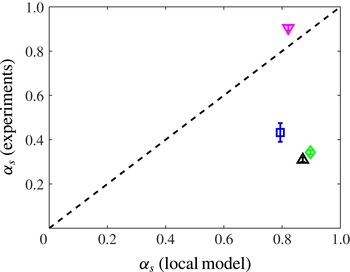
This new functional form, with $v_{0}$ and $L_{0}$ as free fitting parameters, does not fit the experiments. Actually, there is a major discrepancy with the relative slip; setting $y=H/2$ in (4.11) and using the definition (4.2) of the relative slip, we obtain

(4.12) $$\begin{eqnarray}{\it\alpha}_{s}={\displaystyle \frac{1}{1+{\displaystyle \frac{h}{2L_{0}}}\coth {\displaystyle \frac{H}{2L_{0}}}}}\simeq \frac{1}{1+h/2L_{0}},\end{eqnarray}$$

since $\coth (H/2L_{0})$ is very close to 1 for all our experiments. This prediction is much higher than the experimental value, except for the wet foam (figure 6).

Figure 6.

Relative slip measured in the experiments described in table 1, as a function of the relative slip (4.12) predicted by the local model.

4.2.2. Nonlinear model

A possible reason for the discrepancy lies in the fact that the wall friction force is nonlinear in velocity, and the bulk viscous stress is nonlinear in shear rate. Following Denkov et al. (Reference Denkov, Tcholakova, Golemanov, Ananthapadmanabhan and Lips2009), the bulk viscous stress for a 3D foam equals ${\it\sigma}=({\it\tau}_{\mathit{VF}}+{\it\tau}_{\mathit{VS}}){\rm\Gamma}/R$ (film and interface contribution respectively), with $R$ the bubble radius and

(4.13) $$\begin{eqnarray}{\it\tau}_{\mathit{VF}}=1.16\text{Ca}_{\dot{{\it\gamma}}}^{0.47}(1-{\it\phi}_{l})^{5/6}\frac{(0.26-{\it\phi}_{l})^{0.1}}{{\it\phi}_{l}^{0.5}},\end{eqnarray}$$

with $\text{Ca}_{\dot{{\it\gamma}}}={\it\mu}\dot{{\it\gamma}}R/{\rm\Gamma}$ the capillary number ( ${\it\mu}=10^{-3}~\text{Pa}~\text{s}$ : bulk viscosity) and ${\it\tau}_{\mathit{VS}}=9.8{\rm\pi}B\dot{{\it\gamma}}^{0.18}$ with $B=2.12\times 10^{-3}$  S.I. an empirical constant for SLES/CAPB/MAc foams. Using as orders of magnitude from the experiments $R\approx \sqrt{A/{\rm\pi}}\approx 2~\text{mm}$ and $\dot{{\it\gamma}}\approx v_{0}/L_{v}\approx 1~\text{s}^{-1}$ , we obtain ${\it\tau}_{\mathit{VS}}/{\it\tau}_{\mathit{VF}}\approx 0.6$ , hence the film term is dominant, although the surface term is not negligible. Keeping only the film term for simplicity, (4.13) shows that the bulk viscous stress scales sublinearly with the shear rate:

(4.14) $$\begin{eqnarray}{\it\sigma}={\it\eta}^{\prime }\dot{{\it\gamma}}^{0.47},\end{eqnarray}$$

where the prefactor ${\it\eta}^{\prime }$ (primed to distinguish it from the plastic viscosity in the linear law used in § 4.2.1) is

(4.15) $$\begin{eqnarray}{\it\eta}^{\prime }=1.16\frac{{\it\mu}^{0.47}{\rm\Gamma}^{0.53}}{R^{0.53}}(1-{\it\phi}_{l})^{5/6}\frac{(0.26-{\it\phi}_{l})^{0.1}}{{\it\phi}_{l}^{0.5}}.\end{eqnarray}$$

For solutions giving rigid interfaces, like SLES/CAPB/MAc (Golemanov et al. Reference Golemanov, Denkov, Tcholakova, Vethamuthu and Lips2008), foam/wall friction is quantified by the force per unit area (or equivalently the wall stress) (Denkov et al. Reference Denkov, Tcholakova, Golemanov, Ananthapadmanabhan and Lips2009):

(4.16) $$\begin{eqnarray}f_{D}=\frac{{\rm\Gamma}}{R}\left[1.25C_{IF}\sqrt{\text{Ca}^{\ast }}\sqrt{\frac{F_{3}}{1-F_{3}}}+2.1C_{IL}(\text{Ca}^{\ast })^{2/3}\right]F_{3},\end{eqnarray}$$

with two empirical constants $C_{IF}=3.7$ and $C_{IL}=3.5$ , $\text{Ca}^{\ast }={\it\mu}v/{\rm\Gamma}$ another capillary number, and

(4.17) $$\begin{eqnarray}F_{3}=\sqrt{1-3.2\left(\frac{1-{\it\phi}_{l}}{{\it\phi}_{l}}+7.7\right)^{-1/2}}.\end{eqnarray}$$

For $v\approx 1~\text{cm}~\text{s}^{-1}$ , the ratio of the second term to the first term in (4.16) is 5, hence we neglect the second term. Equation (4.16) then shows that the wall friction force scales sublinearly with the velocity:

(4.18) $$\begin{eqnarray}f_{D}=-{\textstyle \frac{1}{2}}h{\it\beta}^{\prime }\sqrt{v},\end{eqnarray}$$

with the following value of the wall friction constant (primed to distinguish it from its counterpart in the linear law used in § 4.2.1):

(4.19) $$\begin{eqnarray}{\it\beta}^{\prime }=\frac{2.5C_{IF}}{hR}\sqrt{{\rm\Gamma}{\it\mu}}\sqrt{\frac{F_{3}^{3}}{1-F_{3}}}.\end{eqnarray}$$

Like in § 4.2.1, see (4.7), we can construct a characteristic length from ${\it\eta}^{\prime }$ and ${\it\beta}^{\prime }$ . To do so, it is convenient to replace the exponent 0.47 by $1/2$ in (4.14), recasting the factor $\dot{{\it\gamma}}^{0.03}$ in the definition (4.15) of ${\it\eta}^{\prime }$ ; this factor is almost constant, and equal to 1, for all our experiments. The characteristic length is then $L_{0}^{\prime }=({\it\eta}^{\prime }/{\it\beta}^{\prime })^{2/3}$ . It is the extension the friction length $L_{0}$ defined in (4.7) to the case of the nonlinear wall friction (4.18) and the nonlinear bulk viscous stress (4.14). We compute with all the experimental values of the parameters appearing in (4.15) and (4.19): $L_{0}^{\prime }=1.9~\text{mm}$ for ${\it\phi}_{l}=4.8\,\%$ and 2.7 mm for ${\it\phi}_{l}=16.9\,\%$ . These orders of magnitude are compatible with the experimental values of the localisation lengths (table 1).

The effect of nonlinear wall friction and bulk viscous stress on the velocity profile has been theoretically considered for Couette flows (Weaire et al. Reference Weaire, Hutzler, Langlois and Clancy2008; Weaire, Clancy & Hutzler Reference Weaire, Clancy and Hutzler2009), but not for Poiseuille flows. Therefore, in appendix C, we compute analytically the velocity profile using the nonlinear laws (4.14) and (4.18), and we show that the role of these nonlinearities on the velocity is negligible.

Hence, the present model is too simple to capture wall slip in our experiments, which suggests that the role of elastic stresses is crucial. This is qualitatively supported by the fact that the only experiment for which the local model is quite accurate in predicting the amount of slip is for a wet foam, which stores less elastic energy (Cantat et al. Reference Cantat, Cohen-Addad, Elias, Graner, Höhler, Pitois, Rouyer and Saint-Jalmes2013). To further support this idea, we plot the shear component of the elastic stress and the normal elastic stress difference in figure 7; see the end of § 2.2 for the measurement of the elastic stress. The shear elastic stress is indeed about four times weaker for the wet foam than for the four other experiments. For these experiments at given bubble area and liquid fraction, its variation across the channel is as follows: towards the centre of the channel, although with a significant asymmetry for some experiments, there is a zone of quasilinear increase around ${\it\sigma}_{xy}^{e}=0$ . The width of this region decreases slightly at increasing flow rate. Outside this region, the elastic shear stress plateaus to a value that does not depend much on the flow rate. Interestingly, there is still some velocity variation, and a significant plastic activity, outside those regions where the shear elastic stress plateaus. Except for the experiment for the wet foam, the normal elastic stress difference ${\it\sigma}_{xx}^{e}-{\it\sigma}_{yy}^{e}$ is always positive, i.e. the bubbles are elongated streamwise, an effect that is clearly visible in figure 1(b). It tends to increase towards the wall.

Figure 7.

(a) Shear component of the elastic stress and (b) normal difference of the elastic stress for the five experiments described in table 1.

Equation (4.3) expresses the balance between the driving pressure gradient, the foam/wall friction and the gradient of elastic and bulk viscous stresses. Close to the middle of the channel, the velocity gradient is very weak, hence bulk viscous stress is negligible, and the gradient of the shear elastic stress is roughly constant (figure 7). It is interesting to compare the value of this gradient $\text{d}{\it\sigma}_{xy}^{e}/\text{d}y$ and the pressure gradient $\text{d}P/\text{d}x$ . Their experimental values are reported in table 1; the pressure gradient is always larger than the gradient of shear elastic stress, the missing part being wall friction. This is a major difference from Poiseuille experiments in 3D channels (Goyon et al. Reference Goyon, Colin, Ovarlez, Ajdari and Bocquet2008, Reference Goyon, Colin and Bocquet2010; Geraud et al. Reference Geraud, Bocquet and Barentin2013), where wall friction is absent. This prevents us from measuring directly the spanwise stress from the pressure gradient, in contrast to the aforementioned studies.

4.3. Numerical simulations and comparison with the fluidity model

We have shown the inaccuracies of a local model without elasticity in capturing our experimental data thanks to the inspection of the boundary condition at the wall. To test the effects of elasticity, local visco-elastoplastic models could be used (Cheddadi et al. Reference Cheddadi, Saramito and Graner2012), but it is not straightforward to deduce testable predictions from them. Moreover, elasticity is not the only aspect of the physics of foams and dense emulsions missed by a model such as that discussed in the previous sections. It has recently been shown in experiments of flowing emulsions in microchannels (Goyon et al. Reference Goyon, Colin, Ovarlez, Ajdari and Bocquet2008) that in order to capture the velocity profiles, the intrinsic non-local rheology of such soft glassy materials must be considered. Non-locality is due to the long-ranged relaxation of stress released after a plastic rearrangement occurs. Building on previous models for soft glassy rheology (Sollich et al. Reference Sollich, Lequeux, Hébraud and Cates1997; Hébraud & Lequeux Reference Hébraud and Lequeux1998; Sollich Reference Sollich1998), Bocquet et al. (Reference Bocquet, Colin and Ajdari2009) proposed a kinetic elastoplastic model (KEP henceforth) to describe explicitly spatial interactions among plastic events. The continuum limit of KEP suggests that the local relation between the stress ${\it\sigma}$ and the rate of strain $\dot{{\it\gamma}}$ is dictated by a kind of inverse effective viscosity, the fluidity

(4.20) $$\begin{eqnarray}f=\frac{\dot{{\it\gamma}}}{{\it\sigma}},\end{eqnarray}$$

which obeys a non-local diffusion–relaxation equation of the form

(4.21) $$\begin{eqnarray}{\it\xi}^{2}{\rm\Delta}f(\boldsymbol{x})+f_{b}({\it\sigma}(\boldsymbol{x}))-f(\boldsymbol{x})=0,\end{eqnarray}$$

where $f_{b}$ is the bulk fluidity, i.e. the value of the fluidity in the absence of spatial cooperativity ( ${\it\xi}=0$ ), and ${\it\xi}$ is the cooperativity length scale within the material due to spatial heterogeneities and represents, basically, a correlation length for the fluidity itself, as can be easily derived from (4.21). The other important result of KEP is that such fluidity must be expected to be proportional to the rate of occurrence of plastic events, $R_{T1}$ , in the system, i.e. $f\propto R_{T1}$ . Furthermore, KEP encompasses the effect of elasticity through the non-local relaxation of elastic stress induced by plastic events. There is, however, a difficulty in testing this non-local model against our experiments. The role of wall friction is crucial in experiments, whereas the non-local model has been set up and tested in its absence, although recent studies have considered the coupled role of wall friction and non-locality (Barry, Weaire & Hutzler Reference Barry, Weaire and Hutzler2011; Scagliarini, Dollet & Sbragaglia Reference Scagliarini, Dollet and Sbragaglia2014). Indeed, wall friction complicates the stress profile across the channel, as discussed in § 4.2, and it is thus not straightforward to extract relevant flow curves ${\it\sigma}(\dot{{\it\gamma}})$ from our experiments. Hence, it is interesting to run numerical simulations, where the wall friction can be set off and tuned at will.

Various sets of numerical simulations have been performed in the $(F_{P},{\it\beta}^{\ast })$ parameter space (see table 2 for the numerical values used), where ${\it\beta}^{\ast }$ is the value of the friction coefficient (3.8) ${\it\beta}$ made dimensionless with the channel width $H$ and viscosity ${\it\eta}$ , i.e.

(4.22) $$\begin{eqnarray}{\it\beta}^{\ast }=\frac{{\it\beta}H^{2}}{{\it\eta}}=\frac{H^{2}}{L_{0}^{2}},\end{eqnarray}$$

where the last equality is based on the definition of the friction length $L_{0}$ given in (4.7). A flat velocity profile in the bulk is shown by all curves (figure 8), including the case with ${\it\beta}^{\ast }=0$ , witnessing the presence of a non-trivial bulk rheology (Goyon et al. Reference Goyon, Colin, Ovarlez, Ajdari and Bocquet2008, Reference Goyon, Colin and Bocquet2010; Geraud et al. Reference Geraud, Bocquet and Barentin2013). We also report the experimental velocity profile with flow rate $152.5~\text{ml}~\text{min}^{-1}$ (see table 1), just to show that we are able to tune the wall friction parameters in the numerics to achieve the same localisation as observed in the experiments for which an equivalent wall friction parameter ${\it\beta}^{\ast }\approx 250$ can be estimated based on the wall friction constant (4.19) and the plastic viscosity (4.15). While a direct comparison of experiments and numerics in terms of velocity profiles is complicated by boundary conditions (as observed in the experimental data of figure 5, slippage is found to occur at the surfaces of the experiments, while the numerical simulations are performed by imposing no-slip at the walls), an important insight will be provided by simulations for validation of the picture of the plastic flow (§ 4.4) for different values of the wall friction constant, which is a freely tunable parameter in the numerical model, unlike in experiments.

Figure 8.

Numerical velocity profiles, normalised by the centreline velocity $v_{0}$ , for different values of the wall friction constant. Data from three sets of simulations are shown with dimensionless wall friction parameter (see (4.22))  ${\it\beta}^{\ast }=0,100,200$ (runs P1-3 in table 2); the experimental velocity profile with flow rate $152.5~\text{ml}~\text{min}^{-1}$ (see table 1) is also reported to show that we are able to tune the wall friction parameters in the numerics to achieve the same localisation as observed in the experiments. The equivalent ${\it\beta}^{\ast }$ in the experiments is ${\it\beta}^{\ast }\approx 250$ (see text for details). On the abscissae, the $y$ -location across the channel has been normalised by the total channel height.

Figure 9(a) indeed provides some indications that wall friction does not seem to dramatically affect the distribution of plastic events. There we plot the rate of plastic rearrangements, normalised by the total number of events, from experiments and numerics (for the three values of ${\it\beta}^{\ast }$ ). The data show a moderately good collapse onto each other. At a given driving pressure drop, an increase in wall friction results in a decrease of the total number of plastic events $N_{T_{1}}$ . We could estimate the number $N_{T_{1}}$ in the numerical simulations, and it is reported in figure 9(b): for the same simulation time (see caption of table 2) plastic events diminish from $N_{T_{1}}\sim 6\times 10^{3}$ to $N_{T_{1}}\sim 2\times 10^{3}$ on increasing ${\it\beta}^{\ast }$ from 0 to 400. A similar trend is observed for the centreline velocity, which is reported in the inset of figure 9(b). To make this statement more quantitative, we notice that the overall decrease in the number of plastic events can be well captured by the function

(4.23) $$\begin{eqnarray}G({\it\beta}^{\ast })=\frac{2b^{2}N_{T1}^{(0)}}{{\it\beta}^{\ast }}\left[1-\frac{1}{\cosh (\sqrt{{\it\beta}^{\ast }}/b)}\right]\!,\end{eqnarray}$$

a scaling behaviour that can be obtained from the expression of the centreline velocity, $v_{0}$ in (4.1), with ${\it\alpha}_{s}=0$ (no-slip boundary condition for the numerics). The parameter $N_{T1}^{(0)}$ in (4.23) sets the number of plastic events in the limit ${\it\beta}^{\ast }\rightarrow 0$ , whereas the argument $\sqrt{{\it\beta}^{\ast }}/b$ of the hyperbolic function in (4.23) is inversely proportional to the velocity localisation length. The choice of (4.23) as a fitting function is suggested by the consideration that the total number of plastic events is dominated by events occurring in boundary regions where the shear stress is approximately constant and, hence, the fluidity $f$ is basically proportional to the shear rate $\dot{{\it\gamma}}$ . Consequently, as the number of events is, by definition, equal to the integral of the corresponding rate $R_{T1}$ , and since $R_{T1}\propto f\approx |\dot{{\it\gamma}}|$ , we can assume that $G({\it\beta}^{\ast })\propto \int _{0}^{H/2}|\dot{{\it\gamma}}|\text{d}y$ , which equals the centreline velocity. Interestingly, the estimate of $b$ that we obtain from a best fit procedure ( $b\approx 6.0$ ) is greater than the estimate of $b$ based on the friction length $L_{0}$ in (4.7), which would yield $b=2$ . This is an indication that the velocity localisation length in the numerical simulations is larger than the localisation length induced by the wall friction, $\boldsymbol{F}_{D}=-{\it\beta}\boldsymbol{v}$ . This is not a surprise, because our numerical simulations had already confirmed the presence of a cooperativity length scale (Sbragaglia et al. Reference Sbragaglia, Benzi, Bernaschi and Succi2012), without wall friction, in a Couette flow set-up. This supports the idea that an effective localisation length results from the combination of the friction length and the cooperativity length (Barry et al. Reference Barry, Weaire and Hutzler2011), an issue that we will further explore in § 4.4.

Figure 9.

(a) Plot of the rate of plastic rearrangements as a function of $y$ : experiments (▵ in table 1) are compared with numerical data from runs P1–3. The dashed line indicates the function $\sinh (y/L_{v})/y$ , representing the fluidity profile based on the hyperbolic cosine fit of the velocity profile (see § 4.1 for details). Numerical data have been symmetrised. (b) Total number of T1s as a function of ${\it\beta}^{\ast }$ from the simulations; the dashed line is a fit with the functional form given in (4.23). Inset: the centreline velocity versus ${\it\beta}^{\ast }$ is reported.

The study of the spatial distribution in the number of plastic events and the simultaneous analysis of the localisation in the velocity profiles allows us to bridge the gap between the ‘microscopic’ details of local irreversible plastic rearrangements and the macroscopic flow. A connection between the rate of T1 events and the fluidity field is indeed visible in figure 9(a). The dashed line indicates $\sinh (y/L_{v})/y$ , which is the ‘synthetic’ fluidity profile (up to an unessential numerical scaling factor) based on the hyperbolic cosine fit of the velocity profile (see § 4.1) and a linear variation of the shear stress across the channel. Interestingly, a significant plastic activity remains towards the centre of the channel, and it is well correlated to the fluidity field, which remains finite in such regions, whereas the strain rate goes to zero. Moreover, a closer inspection reveals that the decrease in the number of plastic events is affected by the wall friction constant ${\it\beta}^{\ast }$ , with a steeper decrease associated with the larger ${\it\beta}^{\ast }$ . Figure 9 calls, therefore, for a deeper understanding with regard to the link between the rate of plastic events and the local flow properties.

4.4. Localisation lengths: comparison of plasticity and shear rate

To go further, we choose to explore the connection between the rate of plastic events and the local flow properties, by looking at the relationship between the localisation length of the velocity profiles, $L_{v}$ , and the localisation length of the number of plastic events, $L_{p}$ (henceforth called the plastic localisation length). This connection enables us to compare experiments and simulations, despite their different boundary conditions. The velocity localisation length $L_{v}$ is estimated by a hyperbolic cosine function $\cosh (y/L_{v})$ , from which the decay length $L_{v}$ is extracted (see § 4.1). Simultaneously, the plastic localisation length $L_{p}$ is computed out of an exponential fit of the symmetrised rate of plastic events close to the wall (figure 10 a). Since our numerical simulations have already confirmed the presence of a cooperativity length scale (Sbragaglia et al. Reference Sbragaglia, Benzi, Bernaschi and Succi2012) without wall friction, they are good candidates to complement the experimental findings, showing how the spatial distribution of plastic events is affected by a change in the wall friction parameter ${\it\beta}$ . Hence, in figure 10(b) we also look at the localisation in the numerics, by fixing the pressure gradient and changing ${\it\beta}^{\ast }$ , something that cannot be easily done in experiments with the data at hand. At fixed pressure gradient, we show the log–lin plot of the rate of plastic events from simulations with different ${\it\beta}^{\ast }$ . The extracted $L_{p}$ is found to be a decreasing function of ${\it\beta}^{\ast }$ .

Figure 10.

(a) Decimal logarithm of the density of T1s per unit time and area as a function of $y/H$ , for the five experiments described in table 1. These data have been symmetrised with respect to the centreline; the error bars denote the standard deviation resulting from this averaging. Data below $10^{-4}~\text{mm}^{-2}~\text{s}^{-1}$ are not shown because they are statistically irrelevant (fewer than 10 T1s counted per bin per experiment). Dashed lines represent the linear fits of the data. (b) Data from numerical simulations complement the experimental results reported in (a). In particular, to appreciate the effect of wall friction at fixed pressure gradient, we show the log–lin plot of the rate of plastic events from simulations P1–3 (fixed pressure drop and different ${\it\beta}^{\ast }$ ) close to the bottom wall (the dashed lines represent best linear fits of the data). Inset: plastic localisation length as a function of the wall friction parameter ${\it\beta}^{\ast }$ .

In figure 11 we report a scatter plot of the velocity localisation length $L_{v}$ versus the plastic localisation length $L_{p}$ for three sets of data: experiments (symbols as in table 1), simulations with fixed pressure drop and various values of ${\it\beta}^{\ast }$ (filled squares) and simulations with fixed ${\it\beta}^{\ast }=200$ and various pressure drops (filled circles). Figure 11 shows that the two localisation lengths are indeed close to each other. The fact that the values of $L_{p}$ and $L_{v}$ agree confirms the picture of the ‘plastic flow’; it is also compatible with the fact that the rate of plastic events and the fluidity seem to be proportional (§ 4.3).

Barry et al. (Reference Barry, Weaire and Hutzler2011) have combined the local model presented in § 4.2 with the non-local equation for the fluidity field (4.21), in the case of a Couette flow with linear laws for the bulk viscous stress and wall friction (as in § 4.2.1). They predicted that the velocity localisation length is an increasing function of both the cooperativity length ${\it\xi}$ and the friction length $L_{0}$ defined by (4.7). Here, this theoretical prediction can be tested for the first time versus our experiments and simulations. Some care is required in doing so because of the nonlinear nature of wall friction and bulk viscous stress in experiments, and the difference between Couette and Poiseuille flows. However, we have shown in appendix C that the effect of nonlinear wall friction and bulk viscous stress is very weak. Since the velocity localisation length $L_{v}$ is much smaller than the channel width and the stress does not vary much across the localisation zone, the comparison with the Couette predictions is relevant. For this reason, we also repeated some numerical simulations in a Couette flow geometry (see table 2). The associated data nicely collapse onto the same master curve, stressing even more the robustness of our findings on changing the load conditions.

In experiments, at given liquid fraction and bubble area, the localisation length $L_{v}$ increases with increasing flow rate. Moreover, table 1 shows that at given flow rate (up to 5 %) and bubble area, the localisation length is lower for a wet foam than for a dry one, in qualitative agreement with the experiments of Goyon et al. (Reference Goyon, Colin and Bocquet2010) on emulsions. We tried to get further insight into these findings, by investigating the local effect of single plastic events, namely by measuring the way they affect displacement and elastic stress fields on their surroundings, in the spirit of Picard et al. (Reference Picard, Ajdari, Lequeux and Bocquet2004) in theory and Chen, Desmond & Weeks (Reference Chen, Desmond and Weeks2012) in experiments. Our hope was to directly evidence the cooperativity length as the range of influence on displacement and stress fields of single plastic events, and whether it would depend on the flow rate and liquid fraction. However, the data turned out to be too noisy to address this specific question, in particular because of the difficulty in properly subtracting the effect of the mean flow. Hence, we cannot directly measure the cooperativity length. In some sense, the work presented here bypasses the problem of an accurate measurement of the cooperativity length, but directly explores the link between localisation phenomena in the velocity profiles and the rate of plastic events.

Figure 11.

Scatter plot of the velocity localisation length $L_{v}$ (computed from a hyperbolic cosine fit of the velocity profiles) versus the plastic localisation length $L_{p}$ (computed out of an exponential fit of the symmetrised rate of plastic events across the channel) for three sets of data: experiments (symbols as in table 1), simulations of Poiseuille flow with fixed pressure drop and various values of the normalised friction coefficient ${\it\beta}^{\ast }$ (filled squares) and with fixed ${\it\beta}^{\ast }=200$ and various pressure drops (filled circles) and simulations of Couette flow at two values of ${\it\beta}^{\ast }$ (filled triangles); both lengths are normalised by the mean bubble diameter. The dashed line is the $L_{v}=L_{p}$ curve.

4.5. Orientation of the plastic events

The importance of plastic rearrangements has been stressed in that the occurrence of these events induces long-range correlations within the soft glassy material. It is also acknowledged (Picard et al. Reference Picard, Ajdari, Lequeux and Bocquet2004; Schall, Weitz & Spaepen Reference Schall, Weitz and Spaepen2007) that T1s possess a non-trivial angular structure with a quadrupolar topology. It seems, then, reasonable to argue that for a full understanding of the way they determine non-local effects inside the system, not only the distribution of their locations in space but also their orientational properties need to be addressed. Therefore, we go further with the description of plastic events, and study their angular statistics from experiments and simulations. More precisely, focusing on the four bubbles involved in a T1, we define as a disappearing link the segment connecting the centres of the two bubbles that were in contact before the event (and which are then far apart), and as an appearing link the connector between the other two bubble centres (see also § 2 and figures 2 and 3). We then measure for each event the angle between such links and the flow direction. We have observed that the angles are reversed between the two sides of the channel, consistently with the fact that $y=0$ is an axis of symmetry. Therefore, we choose to analyse the statistics of the quantities ${\it\theta}_{d}={\it\theta}_{d}^{\prime }\,\text{sign}\,(y)$ and ${\it\theta}_{a}=\,{\it\theta}_{a}^{\prime }\text{sign}\,(y)$ (see figure 1 for the sign convention of $y$ ). We did not observe a significant variation of the distribution of these angles across the channel, hence we analyse the distributions of these angles for all T1s, whatever their location across the channel. Figure 12 shows the histogram of ${\it\theta}_{d}$ and ${\it\theta}_{a}$ for one experiment and one simulation, while the average and standard deviations of these quantities are summarised for all experiments in table 1. This analysis shows that T1s have preferential orientations: ${\it\theta}_{d}$ is peaked around 0.5 rad, with a small dispersion, and ${\it\theta}_{a}$ around $-0.7~\text{rad}$ , with a larger dispersion. The average values do not depend significantly on the flow rate. For the wet foam, ${\it\theta}_{d}$ is larger, and ${\it\theta}_{a}$ slightly smaller.

Figure 12.

Normalised distributions of the orientations of plastic events. Distributions of appearing (a) and disappearing (b) centre-to-centre links of bubbles involved in rearrangements are shown, from experiment (thin blue line) and simulations (thick red line). Here, ${\it\theta}$ denotes the angle formed by the link and the direction of the flow, i.e. the positive $x$ -axis. Following Princen (Reference Princen1983), the extreme values are found for a dry foam at liquid fraction ${\it\phi}_{l}=0$ and are indicated with a dashed line.

We now derive some reference values for these angles from a microstructural analysis. Since our foams are rather monodisperse, it is interesting to use the simple geometrical model of a sheared 2D hexagonal foam (Princen Reference Princen1983) (see also Khan & Armstrong Reference Khan and Armstrong1986). In this model, the unit cell drawn in dashed lines in figure 13 is sheared, and the locations of the vertices are computed to comply with the equilibrium rule that the three edges meet at equal angles. To account for the finite liquid fraction, the vertices are decorated with Plateau borders for which the radius $R_{P}$ is an increasing function of the liquid fraction (figure 13 a), ${\it\phi}_{l}=(2\sqrt{3}-{\rm\pi})R_{P}^{2}/A_{h}$ , with $A_{h}$ the area of one hexagon. This structure can be sheared up to the point where two neighbouring Plateau borders meet, which defines the onset of the T1 (figure 13 b).

Figure 13.

Portions of unsheared (a) and sheared (b) hexagonal foam. The strain is defined as ${\it\gamma}=4{\rm\Delta}x/3a$ .

The two angles ${\it\theta}_{a}^{\prime }$ and ${\it\theta}_{d}^{\prime }$ can be computed from simple geometry, when the two Plateau borders come into contact (figure 13 b). The length of the edge $c$ between the two bubbles about to detach is equal to $R_{P}$ . Now, at a given strain ${\it\gamma}$ , this length is (Khan & Armstrong Reference Khan and Armstrong1986) $c=a(1-{\it\gamma}\sqrt{3}/2)/\sqrt{4+{\it\gamma}^{2}}$ , where $a$ is the side length of the undeformed hexagon. Setting $c=R_{P}$ in the latter equation yields the strain ${\it\gamma}_{c}$ at which the T1 occurs; ${\it\gamma}_{c}$ is a decreasing function of $R_{P}$ . Moreover, ${\it\gamma}=1/\sqrt{3}-\cot {\it\alpha}$ (Princen Reference Princen1983), and we compute from geometrical considerations in figure 13(b) $\cot {\it\theta}_{d}^{\prime }=2/\sqrt{3}-\cot {\it\alpha}=1/\sqrt{3}+{\it\gamma}_{c}$ and $\cot {\it\theta}_{a}^{\prime }=-2/\sqrt{3}-\cot {\it\alpha}=-\sqrt{3}+{\it\gamma}_{c}$ . Qualitatively, these two expressions show that both ${\it\theta}_{d}^{\prime }$ and ${\it\theta}_{a}^{\prime }$ are decreasing functions of ${\it\gamma}_{c}$ , hence increasing functions of $R_{P}$ , hence of the liquid fraction. The extreme values are found for a dry foam at ${\it\phi}_{l}=0$ , for which ${\it\gamma}_{c}=2/\sqrt{3}$ (Princen Reference Princen1983), and for the jamming transition for which ${\it\gamma}_{c}=0$ : ${\it\theta}_{d}^{\prime }$ varies between ${\rm\pi}/6\simeq 0.52$  rad (dry foam) and ${\rm\pi}/3\simeq 1.05~\text{rad}$ ( jamming transition), and ${\it\theta}_{a}^{\prime }$ between $-{\rm\pi}/3$ and $-{\rm\pi}/6$ . Our measured values are indeed in these ranges. The values of the disappearing angles for the four experiments with ${\it\phi}_{l}=4.8\,\%$ are compatible (within experimental dispersion) with the dry foam prediction, the latter indicated with a vertical dashed line in figure 12. The predicted increase of the angles with liquid fraction is compatible with the experiments for ${\it\theta}_{d}$ , but not for ${\it\theta}_{a}$ .

Although the model by Princen (Reference Princen1983) gives useful reference values, it is difficult to make a more quantitative comparison based on liquid fraction, because the distribution of liquid is specific to each system. In simulations, the films between droplets are thick, and contain a significant proportion of the liquid. In experiments, the distribution of water is complex because of the 3D structure of the bubbles; there is relatively more water close to the confining plates than in the midplane in between (Cox & Janiaud Reference Cox and Janiaud2008). The hexagonal foam model of Princen (Reference Princen1983) is a good approximation of the structure of our experimental foams across the midplane between the top and bottom confining plates, but the liquid fraction across this plane, relevant in the hexagonal model, is significantly lower than the experimental liquid fraction. Moreover, the measurement of the appearing angle is less precise than that of the disappearing one, because the relaxation of the four bubbles after a T1 is fast; hence, the measurements made on the image after the topological rearrangement may not be representative of the configuration at the instant of a T1. This also explains why the dispersion is larger for ${\it\theta}_{a}$ than for  ${\it\theta}_{d}$ .