1 Introduction
The observation of deep lens structures in the Canary basin, showing important density and rotation anomalies, was first reported by Armi & Zenk (Reference Armi and Zenk1984). Since then, tens of these huge anticyclones, known as Meddies (Mediterranean eddies), have been observed to form at the exit of the Mediterranean sea, and their properties have been analysed and compared (Richardson, Bower & Zenk Reference Richardson, Bower and Zenk2000). The issue of their longevity is not a trivial one, because Meddies are believed to play a relevant role in the interaction between the Mediterranean sea and the Atlantic ocean (Bashmachnikov et al. Reference Bashmachnikov, Neves, Calheiros and Carton2015). The Great Red Spot constitutes another remarkable example of a long-lived anticyclonic vortex, which has been observed in Jupiter’s atmosphere over hundreds of years (Marcus Reference Marcus1993). Anticyclones are also reported to form in numerical simulations of protoplanetary disks (Barranco & Marcus Reference Barranco and Marcus2005) and claimed to contribute to planet formation, which would indicate a lifetime of the order of millions of years.
A set of four parameters is usually chosen in order to describe these three-dimensional (3-D) objects: their vertical and horizontal length scales
 $H$
and
 $L$
, their internal rotation rate
 $\unicode[STIX]{x1D6FA}_{c}$
and their internal Brunt–Väisälä frequency
 $N_{c}=\sqrt{-(g/\unicode[STIX]{x1D70C})\unicode[STIX]{x2202}_{z}\unicode[STIX]{x1D70C}}$
, where the
 $c$
subscripts refer to values evaluated at the centre of the vortex. Several studies have addressed the problem of predicting the aspect ratio
 $\unicode[STIX]{x1D6FC}=H/L$
as a function of the ambient Coriolis and Brunt–Väisälä frequencies,
 $f$
and
 $N$
, which characterize the unperturbed background flow. It is commonly accepted that these variables should be connected as a result of the quasi-geostrophic balance and hydrostatic balance. A scaling law
 $H/L\sim f/N$
has been considered for a long time (see e.g. McWilliams Reference McWilliams1985; Dritschel, de la Torre Jurez & Ambaum Reference Dritschel, de la Torre Jurez and Ambaum1999; Reinaud, Dritschel & Koudella Reference Reinaud, Dritschel and Koudella2003), which does not depend on the vortex internal properties. Recently Hassanzadeh, Marcus & Le Gal (Reference Hassanzadeh, Marcus and Le Gal2012) proposed a new model where the full set of variables
 $H,L,Ro=\unicode[STIX]{x1D6FA}_{c}/f,N_{c}$
enters in a universal quasi-equilibrium relationship
 $$\begin{eqnarray}\unicode[STIX]{x1D6FC}\equiv \frac{H}{L}=\left(\frac{-Ro(1+Ro)}{N^{2}-N_{c}^{2}}\right)^{1/2}f.\end{eqnarray}$$
This relationship has been validated by numerical simulations (Hassanzadeh et al.
Reference Hassanzadeh, Marcus and Le Gal2012) and observations (Aubert et al.
Reference Aubert, Le Bars, Le Gal and Marcus2012). On the contrary Bashmachnikov et al. (Reference Bashmachnikov, Neves, Calheiros and Carton2015) has observed that the tendency of
 $H/R$
following the Iberian coast northward was not in agreement with (1.1). The aim of the present work is to predict and verify how the full set
 $H,L,Ro,N_{c}$
evolves in time.
We perform experiments with a laboratory rotating stratified flow where anticyclones are generated with the same technique as Hedstrom & Armi (Reference Hedstrom and Armi1988), following the seminal work of Griffiths & Linden (Reference Griffiths and Linden1981). We then measure the evolution of the velocity field in the equatorial plane. Based on the experimental observations, we present an axisymmetric model, in contrast with the 2-D theoretical study of Gill (Reference Gill1981). We observe that the dynamics strongly depends on the combination of both the stratification and the background rotation. As a consequence, the typical vortex evolution is significantly different from studies performed in laboratory flows where just one of the two elements was present. In fact, the stratification suppresses the Ekman pumping which dominates the vortex decay in rotating non-stratified flow (Kloosterziel & van Heijst Reference Kloosterziel and van Heijst1991), while rotation makes the action of momentum dissipation much more convoluted than in the case of a plain stratified flow (Beckers et al. Reference Beckers, Verzicco, Clercx and Van Heijst2001). In our model, secondary circulations, while small, are found to play a crucial role. Our results thus significantly differ from the recent model presented by Ungarish (Reference Ungarish2015), which only accounts for the viscous dissipation of the azimuthal motion.
The paper is organized as follows. In § 2, we describe the experimental and numerical tools that we use in our study. In § 3, we report the main experimental observations, while in § 4, we detail the derivation of our theoretical model. In § 5, we compare theory with both experiments and numerical results. Finally in § 6, we summarize our study and briefly investigate the model application to Meddies.
2 Investigation methods
2.1 Experimental apparatus
We study the time evolution of an isolated anticyclone in a laboratory rotating stratified flow using the same experimental apparatus as Aubert et al. (Reference Aubert, Le Bars, Le Gal and Marcus2012). The flow is produced in a transparent tank (
 $50~\text{cm}\times 50~\text{cm}\times 70~\text{cm}$
) mounted on a rotating table. The tank is filled with salty water linearly stratified in density. The density profile is obtained by the double-bucket method (Oster Reference Oster1965). To measure the density profile we collect small samples of fluid (
 ${\sim}10~\text{ml}$
) at different heights and analyse them with a density-meter Anton Paar DMA 35. In our experiment the Brunt–Väisälä frequency
 $N$
varies between
 $0.82~\text{rad}~\text{s}^{-1}$
and
 $2.47~\text{rad}~\text{s}^{-1}$
. For each experiment we measure the stratification before and after the experiment. Secondary circulations appear during the spin-up process (i.e. when we turn on the rotating table) as a consequence of the non-circular geometry of the tank, and possibly perturb the stratification. Nevertheless we verify that the density profile is not significantly perturbed by the spin-up, injection and spin-down processes i.e. the relative discrepancy is approximately 2 %. The rotating table can turn at up to
 $f/2=10~\text{rad}~\text{s}^{-1}$
but in the present experiments we restrict the cases to
 $f/2=1~\text{rad}~\text{s}^{-1}$
and
 $f/2=0.75~\text{rad}~\text{s}^{-1}$
. The presence of the stratification inhibits the Ekman pumping so the spin-up time (i.e. the time before the entire fluid is in solid body rotation) turns out to be quite long (
 ${\sim}4~\text{h}$
). The anticyclone is generated by the injection of a fixed amount (
 ${\sim}150~\text{ml}$
) of neutrally buoyant fluid at the centre of the tank. The injected fluid is rapidly organized into an anticyclone by the Coriolis force (see e.g. Kloosterziel & van Heijst Reference Kloosterziel and van Heijst1991; Aubert et al.
Reference Aubert, Le Bars, Le Gal and Marcus2012). The injection is made by a thin retractable nozzle immersed in the fluid by a rack mounted on the top of the tank. We fix a small sponge sphere at the end of the nozzle to make the exiting fluid flow as laminar as possible and reduce the mixing with the ambient fluid. In the following we will assume that the density in the centre of the anticyclone was always homogeneous at the end of the injection (e.g.
 $N_{c}(t=0)=0$
). In our experiments, the injection process lasts between 100 and 150 rotations (
 $4\unicode[STIX]{x03C0}/f$
) of the table, while we analyse the evolution of the anticyclone during a typical time of 600–900 rotations after the end of the injection and a short transient of about 25 rotations. The fluid is seeded with (
 $10~\unicode[STIX]{x03BC}\text{m}$
– diameter) hollow glass spheres and a laser sheet illuminates the particles in a thin horizontal plane intercepting the anticyclone at its mid-height (i.e. in the equatorial plane). The flow is then recorded from the top by a
 $4~\text{Mpx}$
camera at a frame rate of
 $10~\text{f.p.s.}$
, and the velocity field is obtained by a particle image velocimetry (hereafter PIV) cross-correlation algorithm (Meunier & Leweke Reference Meunier and Leweke2003). The velocity field is always averaged over a time interval of 5–10 rotations which was estimated to be a time scale well separated from both the short-time oscillations due to experimental noise or waves and the large-time evolution of the global velocity field. We then consider the averaged azimuthal and radial velocity (hereafter just azimuthal and radial velocity when for experiments) at the position where the conditions for PIV were the best (e.g. uniform and sufficiently high lighting). The error in determining the azimuthal velocity is estimated looking at its variations over a quadrant at constant radius, and it is approximately 5 %. The injected fluid is also dyed with rhodamine in order to localize the vortex during the injection and adjust the position of the horizontal laser sheet once it is formed.
2.2 Direct numerical simulations
Complementary axisymmetric direct numerical simulations (DNS) were performed using the finite-element solver Comsol Multiphysics. Boussinesq Navier–Stokes equations and an advection–diffusion equation for the density field are solved in the frame rotating at a constant velocity
 $f/2$
, with an imposed linear stably stratified background density along the rotation axis, characterized by the buoyancy frequency
 $N$
. Initial conditions are given by a Gaussian vortex in cyclo-geostrophic balance, i.e. the initial azimuthal velocity is given by
 $$\begin{eqnarray}v=Ro_{0}\,fr\cdot \exp (-r^{2}/L_{0}^{2}-z^{2}/H_{0}^{2}),\end{eqnarray}$$
with the pressure and density fields computed following the cyclo-geostrophic and hydrostatic equations respectively, and zero radial and vertical velocities. In particular each simulation is initialized with zero stratification at the centre of the vortex, in agreement with experiments,
 $N_{c}(t=0)=0$
.
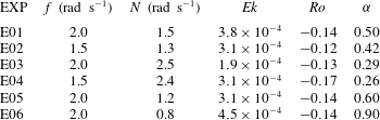
Parameters and initial conditions for a set of 6 laboratory experiments about 25 rotations after the end of the injection. The value of the Schmidt number is estimated to be
 $Sc\sim 700$
for all experiments. Here the value of
 $\unicode[STIX]{x1D6FC}$
is deduced from (1.1), because in the present experiments
 $H$
cannot be measured directly. We make the hypothesis that the core of the anticyclone is initially uniform in density, e.g.
 $N_{c}(t=0)=0$
.

The computation domain is 10 times larger than the characteristic width of the initial vortex
 $L_{0}$
. Only the upper half of the solution is computed, using symmetry conditions around the equatorial plane. The other boundary conditions are no stress and zero density perturbation on the top and equatorial boundaries and no stress and no density flux on the side boundaries. We use standard triangular Lagrange elements of type P2-P3 (i.e. quadratic for the pressure field and cubic for the velocity and density fields). The total number of degrees of freedom is close to 2 million, with a refined mesh in the region of interest. At each time step, the system is solved with the backward difference formulae (BDF) temporal solver and the sparse direct linear solver PARDISO. No stabilization technique is used.
3 Experimental observations
We performed six different experiments for different values of
 $N$
and
 $f$
; parameters are listed in table 1. The value of
 $N/f$
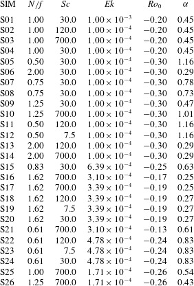
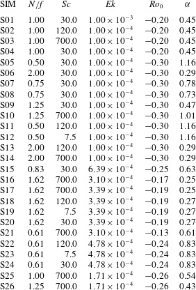
varies by a factor 4 over the whole set of experiments. We also performed DNS in order to compare to the laboratory experiments as well as to extend our study to a wider region of the parameters space. In table 2 we list the parameters and initial conditions for a collection of 27 DNS. Experimentally, we measure the velocity field in the equatorial plane of the anticyclone, during the whole evolution.
Parameters and initial conditions for the whole set of DNS. The initial velocity profile is always Gaussian as in (2.1). The absolute stratification at the centre of the vortex is initially
 $N_{c}=0$
. In simulations S01, S04 and S08 the centrifugal term is neglected in the computation of initial conditions in pressure and density.
We are particularly interested in the strength of the vortex, which is usually associated with the Rossby number
 $Ro$
that we introduced in § 1. First of all, we report that for each experiment the flow is observed to be laminar, axisymmetric and mainly in the azimuthal direction. In fact no relevant averaged radial motion can be detected in the limit of our experimental errors. Also the anticyclone is stable and its strength is always observed to decay, i.e.
 $Ro(t)\rightarrow 0$
. This may be in contrast with previous numerical and theoretical studies (Nguyen et al.
Reference Nguyen, Hua, Schopp and Carton2012; Yim Reference Yim2015; Mahdinia et al.
Reference Mahdinia, Hassanzadeh, Marcus and Jiang2016) according to which the region of parameters we explored is unstable. In the experiments E05 and E06 (i.e. when
 $N/f$
is the smallest), the lateral boundaries of the dyed region in a vertical cut are not totally smooth and appear partially jagged. Nevertheless the slow evolution of these features did not allow us to determine whether they were the result of some turbulent mixing produced by the injection or evidence for the existence of an axisymmetric disturbance with a small, non-negative, growth rate. We suspect that in our experiments the
 $Re$
number was not big enough to trigger any instability or, at least, the associated growth rates were too small for having the core of the vortex destabilized, and weak disturbances only affected the periphery of the vortex. This may be consistent with Nguyen et al. (Reference Nguyen, Hua, Schopp and Carton2012) and Mahdinia et al. (Reference Mahdinia, Hassanzadeh, Marcus and Jiang2016) which localised the most unstable mode at the vortex periphery although a direct comparison is made difficult by their fully inviscid approach. Yim (Reference Yim2015) showed the existence of instabilities at finite
 $Re$
number, but no results were presented combining the small
 $Ro$
number (e.g.
 $Ro\sim 0.1$
) and moderate
 $Re$
number (e.g.
 $Re\sim 1000$
) which characterized all our experiments. Also in our experiments the
 $Ro$
evolves in time and a straight comparison with instability analysis at fixed
 $Ro$
may be not appropriate. What was clear (e.g. looking at the dyed region in the equatorial plane) is that for each experiment the core of the anticyclone remained compact and axisymmetric over hundreds of table rotations.
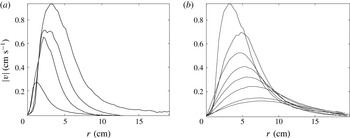
In figure 1 we report the radial profile of the azimuthal velocity
 $v$
, i.e.
 $v(r,z=0)$
, at different times, up to 450 rotations for the experiment E05. Each profile corresponds to the time average over an interval of 5–10 rotations. The experimental error is estimated to be approximately 5 %. The injection process takes approximately a hundred rotations. One recognizes how the injection process (figure 1
a) generates a non-zero azimuthal velocity at progressively larger radius, while the Rossby number (i.e. the slope of the profile at
 $r=0$
) remains relatively constant. After the end of the injection (figure 1
b) the velocity anomaly spreads to even larger radius and the modulus of the Rossby number decreases. We remark that the vortex is still spinning for up to a thousand rotations after the end of the injection. Such a long lifetime and laminar evolution indicates that a viscous mechanism may control the vortex decay. The importance of viscous effects is expressed by the Ekman number
 $Ek=2\unicode[STIX]{x1D708}/L_{0}^{2}f$
whose value is reported in table 1 for each experiment. At this stage we neglect any effect of salt on the viscosity of water and consider
 $\unicode[STIX]{x1D708}$
as the viscosity of pure water at
 $20^{\circ }$
,
 $\unicode[STIX]{x1D708}=10^{-6}~\text{m}^{2}~\text{s}^{-1}$
. The value of
 $L_{0}$
varies between
 $5$
and
 $10~\text{cm}$
, thus a viscous time scale given by
 $T=2/(fEk)$
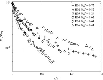
is consistent with the experimental observations reported in figure 2. One clearly sees that irrespective of
 $N/f$
, the Rossby number decreases by more than an order of magnitude over a time of the order of
 $T$
, while the details of this evolution depend on
 $N/f$
and will be studied in the next section.
Absolute value of the azimuthal velocity
 $v$
as a function of radius
 $r$
at
 $z=0$
from experiment E05. (a) For different times before the end of the injection corresponding to
 $t=0$
(injection duration of
 $538~\text{s}$
): from lower to upper curve,
 $t=-484~\text{s}$
,
 $t=-331~\text{s}$
,
 $t=-181~\text{s}$
,
 $t=0~\text{s}$
. (b) For different times after the end of the injection: from upper to lower curve,
 $t=0~\text{s}$
,
 $t=214~\text{s}$
,
 $t=396~\text{s}$
,
 $t=626~\text{s}$
,
 $t=916~\text{s}$
,
 $t=1372~\text{s}$
,
 $t=2255~\text{s}$
,
 $t=2280~\text{s}$
.

Rossby number as a function of time. Different markers correspond to different experiments. The Rossby number is divided by its initial value for each experiment. The time is made non-dimensional by
 $T=L_{0}^{2}/\unicode[STIX]{x1D708}$
where
 $L_{0}$
is determined by a Gaussian fit on the velocity radial profile at time
 $t=0$
, i.e. at about 25 rotations after the end of the injection.

It is well known that a viscous dominated evolution is associated with a diffusion-like equation. According to Kloosterziel (Reference Kloosterziel1990), the solution of a diffusion equation can be decomposed into a sum of fast decaying self-similar solutions, whose self-similar variable reads
 $$\begin{eqnarray}\unicode[STIX]{x1D702}=r/\sqrt{1+4t/T}.\end{eqnarray}$$
(In the work of Kloosterziel (Reference Kloosterziel1990)
 $\unicode[STIX]{x1D702}=r/\sqrt{1+2t/T}$
, because fast decaying functions belong to the the Hilbert space
 $L^{2}(\boldsymbol{R}^{n},\text{e}^{-|x|^{2}/2})$
, while we use
 $\text{e}^{-|x|^{2}}$
.) All these solutions decay at a different rate, which in the end leads to one component (i.e. the slowest in decaying) largely dominating the other ones. When no net vorticity is introduced in the system (i.e. a vortex produced by injection), the leading component of the decomposition coincides with a Gaussian isolated vortex (hereafter Gaussian vortex), frequently used to approximate experimental isolated vortices (Kloosterziel & van Heijst Reference Kloosterziel and van Heijst1991; Beckers et al.
Reference Beckers, Verzicco, Clercx and Van Heijst2001). In this case the velocity profile reads
 $$\begin{eqnarray}v(r,z=0,t)=Ro(t)fr\cdot \exp [-(r/L(t))^{2}].\end{eqnarray}$$
In our experiments the radial profile of
 $v$
always shows an inner core of quasi solid body rotation (e.g.
 $v$
linear in
 $r$
), smoothed at its max and then rapidly decreasing to 0 at a radius larger than a length scale that we identify with
 $L$
. In figure 3 we compare the experimental value of
 $v$
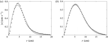
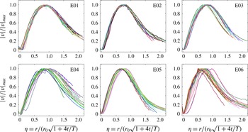
with the best fit of a Gaussian vortex. We observe some minor discrepancy near the maximum and the tail of the velocity profile right after the end of the injection (a) but the agreement improves later in the evolution (b) as predicted by Kloosterziel (Reference Kloosterziel1990). Supported by this first agreement with Kloosterziel’s theory, we can now verify if the velocity profile remains self-similar during the whole evolution. In figure 4 we report the rescaled velocity profiles at different times after the end of the injection. For each profile the velocity is divided by its maximum and the self-similar variable is constructed using the diffusive time scale
 $T=L_{0}^{2}/\unicode[STIX]{x1D708}$
. One remarks that almost all the profiles collapse on the same master curve even if some discrepancies appear when
 $N/f$
significantly deviates from 1 (i.e. E04 and E06).
Absolute value of the azimuthal velocity
 $v$
as a function of the radius
 $r$
at
 $z=0$
. Circles correspond to experimental data, the solid line is the best fit of a Gaussian vortex. (a) Right after the injection. (b)
 $t\sim 0.2T$
.

Superposition of the rescaled velocity profiles as a function of the similarity variable
 $\unicode[STIX]{x1D702}=r/(r_{0}\sqrt{1+4t/T})$
at different times for the whole set of experiments. For each profile the velocity is divided by its maximum.

The above simple diffusive model thus provides a first-order description of our experimental results. To go further, we present below an analytical approach of our system, which allows us to better describe the explicit dependence of the system evolution on
 $N/f$
.
4 A model for the lifetime of a pancake anticyclone
4.1 A single equation for the pressure
We consider a cylindrical coordinate system
 $(r,\unicode[STIX]{x1D703},z)$
which rotates with the angular velocity
 $f/2$
. The Navier–Stokes equations in the Boussinesq approximation read
 $$\begin{eqnarray}\displaystyle & \displaystyle \frac{\unicode[STIX]{x2202}\boldsymbol{v}}{\unicode[STIX]{x2202}t}+(\boldsymbol{v}\boldsymbol{\cdot }\unicode[STIX]{x1D735})\boldsymbol{v}=-\frac{\unicode[STIX]{x1D735}p^{\prime }}{\unicode[STIX]{x1D70C}_{0}}-\frac{\unicode[STIX]{x1D70C}^{\prime }}{\unicode[STIX]{x1D70C}_{0}}g\hat{\boldsymbol{z}}+f\boldsymbol{v}\times \hat{\boldsymbol{z}}+\unicode[STIX]{x1D708}\unicode[STIX]{x1D6FB}^{2}\boldsymbol{v}, & \displaystyle\end{eqnarray}$$
 $$\begin{eqnarray}\displaystyle & \displaystyle \frac{\unicode[STIX]{x2202}\unicode[STIX]{x1D70C}^{\prime }}{\unicode[STIX]{x2202}t}+(\boldsymbol{v}\boldsymbol{\cdot }\unicode[STIX]{x1D735})\unicode[STIX]{x1D70C}^{\prime }-\frac{N^{2}}{g}\unicode[STIX]{x1D70C}_{0}w\hat{\boldsymbol{z}}=k\unicode[STIX]{x1D6FB}^{2}\unicode[STIX]{x1D70C}^{\prime }, & \displaystyle\end{eqnarray}$$
 $$\begin{eqnarray}\displaystyle & \displaystyle \unicode[STIX]{x1D735}\boldsymbol{\cdot }\boldsymbol{v}=0, & \displaystyle\end{eqnarray}$$
where
 $N=\sqrt{\unicode[STIX]{x2202}_{z}\bar{\unicode[STIX]{x1D70C}}(g/\unicode[STIX]{x1D70C}_{0})}$
is the background Brunt–Väisälä frequency,
 $\unicode[STIX]{x1D708}$
and
 $k$
are the viscosity and salt diffusivity and
 $\boldsymbol{v}=(u,v,w)$
is the velocity field. We stress here that
 $\unicode[STIX]{x1D708}$
is intended as a 3-D coefficient (e.g. diffusion is considered as isotropic). The primed variables denote the variations with respect to the stationary unperturbed solution including the linear stable stratification. We refer to
 $p^{\prime }$
and
 $\unicode[STIX]{x1D70C}^{\prime }$
as the pressure and density anomalies, while
 $\bar{\unicode[STIX]{x1D70C}}$
denotes the linear stratification i.e.
 $\unicode[STIX]{x1D70C}(r,z,t)=\unicode[STIX]{x1D70C}^{\prime }(r,z,t)+\bar{\unicode[STIX]{x1D70C}}(z)+\unicode[STIX]{x1D70C}_{0}$
, where
 $\unicode[STIX]{x1D70C}$
is the absolute density and
 $\unicode[STIX]{x1D70C}_{0}$
is a constant.
Based on our experimental observations, a first approximation consists in considering the flow as axisymmetric, i.e. we neglect any
 $\unicode[STIX]{x1D703}$
derivative. Then if one retains only the azimuthal component
 $v$
of the velocity
 $\boldsymbol{v}$
and the viscosity and salt diffusivity are neglected, (4.1) and (4.2) reduce to a time-independent system
 $$\begin{eqnarray}\displaystyle & \displaystyle \frac{\unicode[STIX]{x2202}p^{\prime }}{\unicode[STIX]{x2202}r}=\unicode[STIX]{x1D70C}_{0}v\left(f+\frac{v}{r}\right), & \displaystyle\end{eqnarray}$$
 $$\begin{eqnarray}\displaystyle & \displaystyle \frac{\unicode[STIX]{x2202}p^{\prime }}{\unicode[STIX]{x2202}z}=-\unicode[STIX]{x1D70C}^{\prime }g. & \displaystyle\end{eqnarray}$$
The two equations above describe the cyclo-geostrophic and hydrostatic balances along the horizontal and vertical directions respectively. Hassanzadeh et al. (Reference Hassanzadeh, Marcus and Le Gal2012) showed that a stationary solution exists, which corresponds to a compact isolated vortex centred at
 $r=0$
,
 $z=0$
. The ellipsoidal contour of the vortex is given by the isobars and the aspect ratio
 $\unicode[STIX]{x1D6FC}$
follows the universal law (1.1).
Then we consider the first-order approximation around the quasi-equilibrium state given by the equations (4.4) and (4.5). We assume that terms involving time derivatives and velocities
 $u$
and
 $w$
are small. We also consider small viscous and nonlinear terms, i.e. small Ekman and Rossby numbers:
 $Ek=2\unicode[STIX]{x1D708}/fL^{2}\ll 1$
,
 $Ro\ll 1$
. The azimuthal component of (4.1), equation (4.2) and the incompressibility relation then become
 $$\begin{eqnarray}\displaystyle & \displaystyle \unicode[STIX]{x2202}_{t}v+fu=\unicode[STIX]{x1D708}\unicode[STIX]{x1D6FB}^{2}v, & \displaystyle\end{eqnarray}$$
 $$\begin{eqnarray}\displaystyle & \displaystyle \unicode[STIX]{x2202}_{t}\unicode[STIX]{x1D70C}^{\prime }-\unicode[STIX]{x1D70C}_{0}wN^{2}/g=\frac{\unicode[STIX]{x1D708}}{Sc}\unicode[STIX]{x1D6FB}^{2}\unicode[STIX]{x1D70C}^{\prime }, & \displaystyle\end{eqnarray}$$
 $$\begin{eqnarray}\displaystyle & \displaystyle (1/r)\unicode[STIX]{x2202}_{r}(ru)+\unicode[STIX]{x2202}_{z}w=0, & \displaystyle\end{eqnarray}$$
where we introduced the Schmidt number
 $Sc=\unicode[STIX]{x1D708}/k$
in order to compare the salt diffusion to the momentum dissipation.
Together with (4.4) and (4.5), these form a complete set of linear differential equations.
Now we want to make the problem non-dimensional. As a first step, we fix the azimuthal velocity scale
 $[v]=fL_{0}$
, the length scale
 $[r]=[z]=L_{0}$
and the time scale
 $[t]=T=2/fEk$
. The quasi-equilibrium state equations (4.4) and (4.5) provide the pressure and density scales,
 $[p^{\prime }]=\unicode[STIX]{x1D70C}_{0}f^{2}L_{0}^{2}$
and
 $[\unicode[STIX]{x1D70C}^{\prime }]=\unicode[STIX]{x1D70C}_{0}f^{2}L_{0}/g$
. Finally, the density equation relates the time scale and the vertical velocity scale,
 $[t][w]=L_{0}f^{2}/N^{2}$
, and the divergence-free condition imposes that the vertical and radial velocity scales
 $[w]$
and
 $[u]$
be the same. The equations of motion are now non-dimensional and reduce to
 $$\begin{eqnarray}\frac{\unicode[STIX]{x2202}}{\unicode[STIX]{x2202}t}\left(N_{f}^{2}\unicode[STIX]{x1D6FB}_{r}^{2}p+\frac{\unicode[STIX]{x2202}^{2}p}{\unicode[STIX]{x2202}z^{2}}\right)=N_{f}^{2}\unicode[STIX]{x1D6FB}_{r}^{2}\left(\unicode[STIX]{x1D6FB}_{r}^{2}p+\frac{\unicode[STIX]{x2202}^{2}p}{\unicode[STIX]{x2202}z^{2}}\right)+\frac{1}{Sc}\frac{\unicode[STIX]{x2202}^{2}}{\unicode[STIX]{x2202}z^{2}}\left(\unicode[STIX]{x1D6FB}_{r}^{2}p+\frac{\unicode[STIX]{x2202}^{2}p}{\unicode[STIX]{x2202}z^{2}}\right),\end{eqnarray}$$
where
 $N_{f}=N/f$
,
 $\unicode[STIX]{x1D6FB}_{r}^{2}=(1/r)\unicode[STIX]{x2202}_{r}(r\unicode[STIX]{x2202}_{r})$
and the prime on the
 $p$
variable has been suppressed. The equation above is linear and can be solved in the transformed Hankel–Fourier space. A prediction for the Rossby number can be obtained in the integral form
 $$\begin{eqnarray}\frac{Ro(t)}{Ro_{0}}=\frac{3\unicode[STIX]{x1D6FC}_{0}N_{f}}{2}\int _{0}^{1}\frac{(1-x^{2})\,\text{d}x}{[4t(1-(1-N_{f}^{2})x^{2})(1-(1-1/Sc)x^{2})+\unicode[STIX]{x1D6FC}_{0}^{2}N_{f}^{2}x^{2}+(1-x^{2})]^{5/2}},\end{eqnarray}$$
where the subscript
 $0$
denotes variables at
 $t=0$
. The numerical integration of (4.10) allows us to predict at no cost the time evolution of any pancake vortex in a rotating stratified medium. Also one can solve the equation (4.9) numerically, which provides the pressure anomaly field at any time and then the velocity and density anomaly fields through equations (4.4) and (4.5).
Now, we observe that in the specific case
 $N_{f}=1$
, equation (4.9) greatly simplifies to
 $$\begin{eqnarray}\frac{\unicode[STIX]{x2202}p}{\unicode[STIX]{x2202}t}=\unicode[STIX]{x1D6FB}_{r}^{2}p+\frac{1}{ScN_{f}^{2}}\frac{\unicode[STIX]{x2202}^{2}p}{\unicode[STIX]{x2202}z^{2}},\end{eqnarray}$$
which admits an exact self-similar solution.
Asymptotically, when both the aspect ratio
 $\unicode[STIX]{x1D6FB}_{r}^{2}p/\unicode[STIX]{x2202}_{zz}p\sim \unicode[STIX]{x1D6FC}^{2}$
and the Burger number
 $Bu=N_{f}^{2}\unicode[STIX]{x1D6FC}^{2}$
are small, (4.9) reduces to
 $$\begin{eqnarray}\frac{1}{N_{f}^{2}}\frac{\unicode[STIX]{x2202}p}{\unicode[STIX]{x2202}t}=\unicode[STIX]{x1D6FB}_{r}^{2}p+\frac{1}{ScN_{f}^{2}}\frac{\unicode[STIX]{x2202}^{2}p}{\unicode[STIX]{x2202}z^{2}}.\end{eqnarray}$$
We notice that (4.12) is identical to (4.11) once the time is rescaled by a factor
 $N_{f}^{2}$
, i.e.
 $[t]=T/N_{f}^{2}$
. On the contrary, in the opposite limit
 $\unicode[STIX]{x1D6FB}_{r}^{2}p/\unicode[STIX]{x2202}_{zz}p\gg 1$
and
 $Bu\gg 1$
we recover the equation (4.11). This variety of asymptotic solutions corresponds to a variety of possible behaviours, but also illustrates some generic features. Firstly we observe that in the limit
 $Sc\longrightarrow \infty$
, (4.11) and (4.12) further simplify to a radial diffusion equation of the form
 $$\begin{eqnarray}\frac{\unicode[STIX]{x2202}p}{\unicode[STIX]{x2202}t}=\unicode[STIX]{x1D6FB}_{r}^{2}p.\end{eqnarray}$$
Here we stress that this result does not depend on the aspect ratio
 $\unicode[STIX]{x1D6FC}$
, thus a radial diffusion should occur even for an initial perturbation whose overall shape is already vertically flattened (i.e.
 $\unicode[STIX]{x1D6FC}\ll 1$
). Secondly we observe that the proper limit to neglect the density diffusion, i.e. the rightmost term of (4.11) and (4.12), is
 $$\begin{eqnarray}\frac{\unicode[STIX]{x1D6FB}_{r}^{2}p}{\unicode[STIX]{x2202}_{zz}p}\frac{1}{N_{f}^{2}Sc}\sim \frac{1}{BuSc}\ll 1.\end{eqnarray}$$
Thus, only considering the value of the Schmidt number may be misleading in neglecting or not the density diffusion. Consider for example the case
 $N_{f}=1$
and a moderately low aspect ratio
 $\unicode[STIX]{x1D6FC}=0.3$
: a Schmidt number of order 10 is then expected to significantly impact on the time evolution, which might appear counter-intuitive. A detailed discussion of this effect is given in § 5.4. With regards to our experiments
 $Sc\sim 700$
and thus the limit (4.14) is expected to be fairly valid as long as
 $|Ro|>0.01$
, which according to (1.1), is sufficient to have
 $Bu>0.01$
. In the following we then neglect salt diffusion, even if analytical solutions can also be found with this term.
4.2 Exact and approximate analytic solutions
The equation (4.13) can be solved exactly once the initial condition is given. We consider an initial pressure profile which is Gaussian in both the vertical and the horizontal directions, which is consistent with the measured experimental velocity profile (3.2). The evolution in time reads
 $$\begin{eqnarray}p(r,z,t)=\frac{p_{0}}{1+4t}\cdot \exp [-(r/L(t))^{2}-(z/H(t))^{2}],\end{eqnarray}$$
where
 $L(t)=L_{0}\sqrt{1+4t}$
and
 $H(t)=H_{0}$
, i.e.
 $H$
is constant. This strong anisotropy is uncommon for diffusion-like problems and we claim it follows from the determinant role played by the secondary flow
 $(u,w)$
as will be seen in § 5.3. Also, the explicit time evolution of all the other significant parameters describing the vortex can then be determined analytically
 $$\begin{eqnarray}\displaystyle & \displaystyle Ro(t)=\frac{Ro_{0}}{(1+4t)^{2}}, & \displaystyle\end{eqnarray}$$
 $$\begin{eqnarray}\displaystyle & \displaystyle N^{2}-N_{c}^{2}(t)=\frac{N^{2}-N_{c}^{2}(0)}{1+4t}. & \displaystyle\end{eqnarray}$$
Both the relative rotation and the stratification anomaly (i.e.
 $N^{2}-N_{c}$
) relax to zero, and the aspect ratio
 $H/L$
fulfils the small Rossby version of the scaling law (1.1) at each time.
We stress here that the time dependence of
 $L$
is common to other initial profiles (e.g. as Lamb–Ozeen vortex, Kloosterziel & van Heijst (Reference Kloosterziel and van Heijst1991)), in agreement with the work of Kloosterziel (Reference Kloosterziel1990). On the other hand the functional form for all the other parameters are peculiar to the Gaussian isolated vortex. The compactness and self-similar character of this solution are remarkable but these features are expected only in the particular case
 $N_{f}=1$
and asymptotically in the suitable limit for geophysical applications where
 $\unicode[STIX]{x1D6FC}\ll 1$
and
 $Bu\ll 1$
. The tricky part here is that, even if for
 $\unicode[STIX]{x1D6FC}\ll 1$
, the condition
 $\unicode[STIX]{x1D6FB}_{r}^{2}p\ll \unicode[STIX]{x2202}_{zz}p$
is valid over a large portion of the
 $(r,z)$
plane, there always exists at least a small region, i.e. in the vicinity of
 $\unicode[STIX]{x2202}_{zz}p=0$
, where the approximation is not true. In § 5 we will show how this globally affects the pressure field and prevents the velocity profile from evolving in a truly self-similar way, whenever
 $N_{f}\neq 1$
.
Nonetheless the two limits (4.11) and (4.12) are meaningful irrespective of
 $N_{f}$
and
 $\unicode[STIX]{x1D6FC}$
. We showed that for
 $N_{f}=1$
, the time evolution of
 $Ro$
has the compact form (4.16). Correspondingly, the term
 $1-(1-N_{f}^{2})x^{2}$
in the denominator of integral (4.10) simplifies to
 $1$
, the
 $x^{4}$
dependence is removed, and the integral can be solved analytically. The same analytical solution is also obtained by substituting
 $x^{2}$
in this term by the integral lower bound
 $x=0$
. Equation (4.10) can then be calculated analytically, giving
 $$\begin{eqnarray}\frac{Ro_{1}(t)}{Ro_{0}}=\frac{1}{(1+4t)^{2}}.\end{eqnarray}$$
If we now replace
 $x^{2}$
by the integral upper bound
 $1$
,
 $1-(1-N_{f}^{2})x^{2}$
simplifies to
 $N_{f}^{2}$
and (4.10) is written:
 $$\begin{eqnarray}\frac{Ro_{2}(t)}{Ro_{0}}=\frac{1}{(1+4tN_{f}^{2})^{2}}.\end{eqnarray}$$
One can easily verify that the exact solution
 $Ro(t)$
is bounded by the asymptotic solutions
 $Ro_{1}(t)$
and
 $Ro_{2}(t)$
, and that
 $Ro_{1}(t)$
and
 $Ro_{2}(t)$
correspond to the exact solution of (4.11) and (4.12). Thus even if the evolution is self-similar only for
 $N_{f}=1$
, any other case can always be bounded by two self-similar solutions, which are identical except for a factor
 $N_{f}$
in the time scale.
4.3 Small perturbation approach around
 $N_{f}=1$

Here we want to derive how the solution of equation (4.13) is modified close to
 $N_{f}=1$
. We define a small parameter
 $\unicode[STIX]{x1D716}=N_{f}-1$
and assume the solution can be written as
 $p=p_{0}+\unicode[STIX]{x1D716}p_{1}$
where
 $p_{0}$
corresponds to the self-similar solution (4.15) and
 $p_{1}$
remains to be determined. Substituting in (4.9), with the Schmidt term dropped for now, one finds
 $$\begin{eqnarray}\frac{\unicode[STIX]{x2202}}{\unicode[STIX]{x2202}t}\left(\unicode[STIX]{x1D6FB}_{r}^{2}p_{1}+\frac{\unicode[STIX]{x2202}^{2}p_{1}}{\unicode[STIX]{x2202}z^{2}}\right)=\unicode[STIX]{x1D6FB}_{r}^{2}\left(\unicode[STIX]{x1D6FB}_{r}^{2}p_{1}+\frac{\unicode[STIX]{x2202}^{2}p_{1}}{\unicode[STIX]{x2202}z^{2}}\right)+f(r,z,t),\end{eqnarray}$$
where
 $$\begin{eqnarray}f(r,z,t)=\frac{\unicode[STIX]{x2202}}{\unicode[STIX]{x2202}t}\frac{\unicode[STIX]{x2202}^{2}p_{0}}{\unicode[STIX]{x2202}z^{2}}.\end{eqnarray}$$
We observe that
 $p_{1}$
fulfils the same equation as
 $p_{0}$
at
 $N_{f}=1$
with an additional forcing term
 $f(r,z,t)$
which can be computed explicitly. We cannot find a simple solution because of the forcing term, thus we consider the two limit cases where either
 $\unicode[STIX]{x1D6FB}_{r}^{2}$
or
 $\unicode[STIX]{x2202}_{zz}$
are negligible. When
 $\unicode[STIX]{x1D6FB}_{r}^{2}\ll \unicode[STIX]{x2202}_{zz}$
(in particular close to the axis
 $z=0$
) we end up with
 $$\begin{eqnarray}\unicode[STIX]{x2202}_{t}p_{1}=\unicode[STIX]{x1D6FB}_{r}^{2}p_{1}+\unicode[STIX]{x2202}_{t}p_{0}\end{eqnarray}$$
and when
 $\unicode[STIX]{x1D6FB}_{r}^{2}\gg \unicode[STIX]{x2202}_{zz}$
(i.e. at
 $r=L/\sqrt{2}$
and especially at
 $z=H$
) one has
 $$\begin{eqnarray}\unicode[STIX]{x2202}_{t}p_{1}=\unicode[STIX]{x1D6FB}_{r}^{2}p_{1}+\unicode[STIX]{x2202}_{zz}p_{0},\end{eqnarray}$$
where we have used the fact that
 $\unicode[STIX]{x2202}_{t}\unicode[STIX]{x2202}_{zz}p_{0}=\unicode[STIX]{x1D6FB}_{r}^{2}\unicode[STIX]{x2202}_{zz}p_{0}$
, as
 $p_{0}$
satisfies (4.13). Numerical simulations presented in § 5.1 show that when
 $N_{f}\neq 1$
, the most significant variations appear in the velocity field. Thus we take the radial derivative of the two equations above and solve them for the perturbation of the velocity field, i.e.
 $v_{1}=\unicode[STIX]{x2202}_{r}p_{1}$
as follows from the geostrophic balance. In the first case one finds
 $$\begin{eqnarray}\displaystyle & \displaystyle \unicode[STIX]{x2202}_{t}v_{1}=\frac{\unicode[STIX]{x2202}}{\unicode[STIX]{x2202}r}\left(\frac{1}{r}\frac{\unicode[STIX]{x2202}(rv_{1})}{\unicode[STIX]{x2202}r}\right)+f_{1}(r,z,t), & \displaystyle\end{eqnarray}$$
 $$\begin{eqnarray}\displaystyle & \displaystyle f_{1}(r,z,t)=\frac{\unicode[STIX]{x2202}}{\unicode[STIX]{x2202}t}\frac{\unicode[STIX]{x2202}}{\unicode[STIX]{x2202}r}p_{0}=-\frac{4r(r^{2}-8t-2)\text{e}^{-(z^{2}/H_{0}^{2})-(r^{2}/(4t+1))}}{(4t+1)^{4}}. & \displaystyle\end{eqnarray}$$
In the other limit
 $$\begin{eqnarray}\displaystyle & \displaystyle \unicode[STIX]{x2202}_{t}v_{1}=\frac{\unicode[STIX]{x2202}}{\unicode[STIX]{x2202}r}\left(\frac{1}{r}\frac{\unicode[STIX]{x2202}(rv_{1})}{\unicode[STIX]{x2202}r}\right)+f_{2}(r,z,t), & \displaystyle\end{eqnarray}$$
 $$\begin{eqnarray}\displaystyle & \displaystyle f_{2}(r,z,t)=\frac{\unicode[STIX]{x2202}}{\unicode[STIX]{x2202}z^{2}}\frac{\unicode[STIX]{x2202}}{\unicode[STIX]{x2202}r}p_{0}=\frac{2r(H_{0}^{2}-2z^{2})\text{e}^{-(z^{2}/H_{0}^{2})-(r^{2}/(4t+1))}}{H_{0}^{4}(4t+1)^{2}}. & \displaystyle\end{eqnarray}$$
Looking at (4.24), i.e. close to
 $z=0$
, one sees that the sign of the forcing term
 $f_{1}$
is given by
 $(1-r^{2}/2L^{2}(t))$
, so that the sign of the velocity perturbation (i.e
 $\unicode[STIX]{x1D716}v_{1}$
) is positive (negative) in the exterior (interior) of the vortex for
 $N_{f}<1$
and the opposite for
 $N_{f}>1$
. Similarly, if one looks at (4.26), i.e. close to
 $r=0$
, the sign of
 $f_{2}$
is given by
 $(1-2z^{2}/H^{2})$
. Thus the sign of the velocity perturbation is positive (negative) in the exterior (interior) of the vortex for
 $N_{f}<1$
and the opposite for
 $N_{f}>1$
. Next we compare the predictions of our theoretical model to the experimental and numerical results.
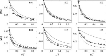
Evolution of the absolute value of the Rossby number as a function of time for a collection of experiments. In each panel we report the experimental results (markers), the exact solution of the linear model (4.10) (solid line) and the two limit solutions
 $Ro_{1}(t)$
(dashed line) and
 $Ro_{2}(t)$
(dotted line). Two series of markers (○ and ♢), corresponding to two distinct radial cuts, are presented to give an estimation of the experimental error.

5 Results and comparison of the experiments, numerics and analytical solution
5.1 Comparison of the experiments with the analytical model
In figure 5 we report the evolution of the Rossby number as a function of time for the whole set of experiments. Experimental results are reported together with the prediction given by the linear model (4.10), and also with the exact solution of the radial diffusion equation in the two asymptotic limits described in the previous section. First of all we verify that the value of the experimental Rossby number (markers) is bounded by the two analytic solutions
 $Ro_{1}(t)$
(dashed line) and
 $Ro_{2}(t)$
(dotted line), which are both of the type (4.16) and differ by a factor
 $N_{f}^{2}$
in the time scale. At the same time, as soon as
 $N_{f}$
significantly deviates from 1, neither of these two limits can provide a quantitative prediction of the value of
 $Ro$
. On the contrary we observe that the numerical solution of the full linear model (solid line) is fairly consistent with the experimental results. We recall here that this prediction demands us to solve numerically the integral (4.10) at only a small computational cost.
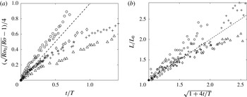
In figure 6(a) we report again the results of all experiments. Here we show the variable
 $\sqrt{Ro_{0}/Ro-1}/4$
, which should be linear in
 $t$
for a diffusive equation, with a slope
 $1$
for the ideal case given by (4.16) (i.e. the straight dashed line). We notice that the Rossby number decays slower (i.e. lower slope) in the case
 $N_{f}<1$
and faster (i.e. higher slope) in the case
 $N_{f}>1$
. This is consistent with the perturbation analysis close to
 $N_{f}=1$
, because close to
 $(r=0,z=0)$
we expect an increase of
 $|v|$
for
 $N_{f}<1$
and a decrease for
 $N_{f}>1$
. Also we observe that far from
 $N_{f}=1$
, the experimental data are poorly fit by a straight line. In figure 6(b) we report the evolution of the horizontal length scale
 $L$
as a function of the time. The values of
 $L$
are obtained by a Gaussian fit to the radial profile of
 $v$
, and time is rescaled according to the exact solution of a radial diffusion equation (3.1) (dashed line). In this case the experimental data are slightly more noisy but we can clearly see that all the experiments spread around the radial diffusion solution in a moderate way. Also we can see that when
 $N_{f}>1$
the radial diffusion is more effective. Again this is in agreement with our small perturbation theory around
 $N_{f}=1$
, which predicts a negative (positive) correction of
 $|v|$
in the interior (exterior) and then an additional flattening of the profile. The opposite reasoning works in the case
 $N_{f}<1$
.
(a) Evolution of the Rossby number as a function of the time for our 6 experiments. Markers legend as in figure 2. (b) Evolution of the horizontal length
 $L$
as a function of time. The value of
 $L$
is obtained from a Gaussian fit to the velocity radial profile at each time. In the two panels the dashed lines correspond to the exact solutions at
 $N_{f}=1$
(4.16) and (3.1).

So far we have focused on the velocity field in the equatorial plane of the vortex because these are the only quantitative data available in our experiments. Also all the limits we considered in our theoretical approach indicate that the dynamics of the system should be mainly in the radial direction as long as the density diffusion does not play an important role. Next we want to verify that this prediction is correct by looking at the results from DNS together with the solution of the linear model.
5.2 Comparison of DNS with the analytical model
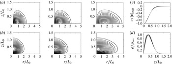
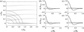
In figure 7 we consider the case
 $N_{f}=1$
,
 $Sc=700$
. In (a) we report the contour plot of
 $v$
in the
 $(r,z)$
plane at three different times. In (c) we superpose the vertical profile of
 $v$
at different times. Such a profile is taken at the value of
 $r$
where
 $|v(r,z=0)|$
is maximum, and all the curves are divided by the maximum value of
 $|v|$
. In (b,d) we report the same graphs for the density anomaly
 $\unicode[STIX]{x1D70C}^{\prime }$
with the only exception that the vertical profile is taken at
 $r=0$
. The contour plots show that the two fields clearly spread only in the radial direction. Also all the vertical cuts collapse on the same master curve, which indicates that the shape of the two fields stays unchanged in the vertical direction. We then confirm that the case
 $N_{f}=1$
can be described as a pure radial diffusion, as long as condition (4.14) is fulfilled.
(a,b) Azimuthal velocity (a) and density anomaly (b) at three different times,
 $t=0.1T$
,
 $t=0.3T$
,
 $t=1.0T$
. Solid contours refer to DNS S25, dashed contours refer to the analytical model. At each time the velocity values are divided by the maximum of
 $|v|$
; contours are reported at a constant step of 0.05. In (c,d) we superpose the values of the azimuthal velocity (c) and density anomaly (d) as a function of
 $z/L_{0}$
at different times between
 $t=0$
(black) and
 $t=T$
(grey). Velocity values are taken at the value of
 $r$
where the velocity is maximum, while density values are taken at
 $r=0$
; the two quantities are divided by their maximum at each time
 $t$
.

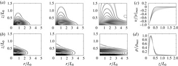
In figure 8 we report the same graphs for the case
 $N_{f}=1.6$
,
 $Sc=700$
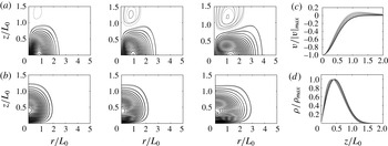
, which is the same as E04. We observe that the core of the vortex still evolves mainly in the radial direction, but some vertical spreading appears in the velocity field. The vertical cuts confirm that some diffusion is acting also in the vertical direction. In figure 9 we consider the case
 $N_{f}=0.61$
,
 $Sc=700$
, which is the same as E05. As in the previous case, the core of the vortex evolves mainly in the radial direction but some new features appear at later times in the velocity field. In this case we observe the formation of a patch of positive vorticity (cyclone) above. The vertical cuts of the velocity field allow us to quantify the strength of this cyclonic cap. At
 $t=T$
the ratio of the Rossby number in the caps to the one in the core is approximately 20 %. Here we stress that the dynamics described in figures 8 and 9 only marginally depends on the density diffusion and on the nonlinear interactions. The first because
 $BuSc>1$
during the whole evolution, the second because our linear model looks consistent with the numerical simulations.
Similar to figure 7, but for S16 where
 $N_{f}=1.62$
.

Similar to figure 7, but for S21 where
 $N_{f}=0.61$
. Positive values of
 $v$
are denoted by dashed-dotted lines (DNS) and dotted lines (analytical model), and reported at a constant step of 0.025.

Looking at figures 8 and 9, the question arises regarding how to define the length scales
 $H$
and
 $L$
, which are supposed to characterize the region of space occupied by the vortex. The question has not been faced so far, because in the case of a self-similar evolution (i.e.
 $N_{f}=1$
) of a Gaussian vortex, the choice is unambiguous. In fact, the pressure, velocity and density fields all share a common Gaussian shape, whose typical lengths are easy to define. When the evolution is not self-similar anymore and the three fields do not show the same shape as seen in figures 8 and 9, the choice is not trivial anymore. From the theoretical point of view the pressure field may be the best candidate because the isopressure lines fairly describe the contour of a Gaussian vortex. On the contrary, this definition is not practical for experiments and observations because the pressure field is not necessarily accessible in a direct way. In this case the best choice is to deduce the value of
 $L$
from the radial profile of the velocity anomaly at
 $z=0$
and
 $H$
from the vertical profile of the density anomaly at
 $r=0$
. Practically, we fit the two profiles with the functional form
 $x\exp -x^{2}/X^{2}$
and take the width
 $X$
as an estimation of the length scale. Alternatively one can estimate the length scale from the position of the maximum. Now, we notice that both the vertical spreading (
 $N_{f}>1$
) and the formation of the cyclonic caps (
 $N_{f}<1$
) do not prevent the core of the velocity anomaly from diffusing radially and barely affect the density field. As a result, we expect
 $L$
and
 $H$
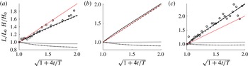
to be weakly sensitive to these phenomena. This is confirmed in figure 10, where we report the values of
 $L$
and
 $H$
as functions of the time for three different values of
 $N_{f}$
and
 $Sc=700$
. We observe that the value of
 $L$
always increases, while
 $H$
is almost constant. In the case
 $N_{f}=1$
we recover exactly the diffusive time law (3.1), while in the case
 $N_{f}<1$
(
 $N_{f}>1$
) the horizontal spreading is lower (faster), in agreement with experiments. In the case
 $N_{f}<1$
the value of
 $H$
even decreases (up to 10 %) as if the initial anticyclone is confined vertically by the formation of the cyclonic caps.
Rescaled value of the horizontal and vertical length scales
 $L$
and
 $H$
as a function of time for
 $N_{f}=0.61$
(a), 1.00 (b) and 1.62 (c). Both
 $L$
and
 $H$
are obtained by a Gaussian fit and divided by their initial values.
 $L$
is deduced from the velocity radial profile at
 $z=0$
and
 $H$
from the vertical density profile at
 $r=0$
. We superpose the value of
 $L$
given by experiments (circles), DNS (solid lines) and the analytical model (dashed lines), as well as the value of
 $H$
given by DNS (dashed-dotted lines) and the analytical model (dotted lines).

5.3 Secondary circulations
As we mentioned in the introduction, previous studies neglected secondary circulations in deriving a model for the decay of a vorticity patch, focusing on the viscous diffusion of the azimuthal velocity (Ungarish Reference Ungarish2015). In our linear model, we do not suppose that
 $u$
or
 $w$
are identically 0 at any stage, while assuming that they are small compared to
 $v$
. In figure 11(a) we superpose the secondary circulation
 $(u,w)$
to the contour plot of the pressure field using results from DNS. We observe an inward vertical flux close to
 $r=0$
and an outward horizontal flux close to
 $z=0$
. The maximum magnitudes are observed inside the vortex and are around
 $0.23L_{0}/T$
for
 $u$
and
 $0.04L_{0}/T$
for
 $w$
. This suggests that the motion associated with
 $(u,w)$
looks more like a slow global deformation of the vortex than a circulation where a fluid particle would travel the same closed path several times. Also this result confirms that
 $u$
and
 $w$
are small compared to
 $v$
, because in these units
 $v$
is of the order of a few hundred.
Next, we want to show that
 $u$
and
 $w$
play a primary role in the time evolution and are responsible for the dominant radial stretching we observe irrespective of the background and initial parameters. In figure 11(b–e) we report all the terms of (4.6), the neglected centrifugal and nonlinear terms as a function of
 $z$
and at a fixed radius
 $r$
. Firstly, we confirm that the leading term is the diffusive one and that the centrifugal term is fairly negligible. Secondly, we observe that the Coriolis term (
 $fu$
) almost compensates the diffusive term, while the time derivative (
 $\unicode[STIX]{x2202}_{t}v$
) is approximately five times smaller. In fact the vertical diffusion of
 $v$
acts primarily on the generation of a non-zero
 $u$
, which in turn is coupled via the divergence equation to
 $w$
which finally advects the density field. As a consequence, we always observe a radial spreading, while for
 $u\equiv 0$
one would expect the diffusion to act mainly along the shortest direction, in order to make the perturbed region isotropic. This result is valid at different radii and times and had already been speculated by Gill (Reference Gill1981). Nevertheless, we remark that a region in
 $z$
always exists where
 $u=0$
, thus the time derivative should be always retained and is also determinant in deriving the final equation for the pressure.
(a) Secondary circulation field
 $(u,w)$
superposed to isolines of the pressure field. Results are from S17 at
 $t/T\sim 0.1$
. The external contour line corresponds to
 $p=p(r=0,z=0,t)/e$
. (b–e) Comparison among the different terms entering the equation for
 $v$
against
 $z$
at a fixed radius. —— diffusion, – – – Coriolis, – - – time derivative,
 $\cdots \cdots$
centrifugal, * nonlinear. (b,c) and (d,e) refer respectively to
 $r/L_{0}=0.1$
and
 $r/L_{0}=0.7$
. (b,d) and (c,e) refer respectively to
 $t/T=0.1$
and
 $t/T=1.0$
.

Finally we want to stress that as long as the geostrophic balance persists, circulations must play a role. In fact, as already noticed by Beckers et al. (Reference Beckers, Verzicco, Clercx and Van Heijst2001), the decay in strength of the vortex caused by momentum dissipation must correspond to a weakening of the pressure anomaly because of the geostrophic balance. The latter demands that the density field should also change. Now, salt diffusion cannot explain this adjustment, because such a response must take place at the viscous time scale. On the contrary, secondary circulations can do it because they act exactly at that time scale.
5.4 The effect of the Schmidt number
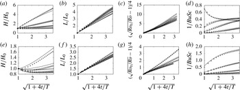
Here we briefly discuss the effect of the Schmidt number. We recall that our theoretical analysis indicates that density diffusion should be neglected only in the limit
 $1/BuSc\ll 1$
. In figure 12 we superpose the results of DNS and the linear model for different values of the Schmidt number (
 $Sc=7.5,30,120,700$
) and two values of
 $N_{f}$
(
 $N_{f}=1.6$
(a–d),
 $N_{f}=0.6$
(e–h)). In (a,e), (b,f), (c,g) we report the evolution of
 $H$
,
 $L$
and
 $Ro$
, while in (d,h) we report the value of
 $1/BuSc$
. We remark that the value of
 $L$
and
 $Ro$
are weakly sensitive to changes in the Schmidt number. On the contrary, the evolution of
 $H$
changes drastically with
 $Sc$
and a vertical diffusion is clearly present below
 $Sc=30$
, corresponding to
 $1/BuSc$
of the order of 0.1–1. We then confirm that
 $1/Sc\ll 1$
is not the relevant parameter to neglect salt diffusion, in contrast to a vortex in a stratified (i.e. non-rotating) flow (Beckers et al.
Reference Beckers, Verzicco, Clercx and Van Heijst2001). The vertical diffusion is much less effective for
 $N_{f}<1$
, which is a consequence of the formation of the cyclonic caps. But in all cases,
 $1/BuSc$
tends to increase at large times because of the radial spreading (i.e.
 $\unicode[STIX]{x1D6FC}$
diminishes), thus some density diffusion always appears at large times. Finally, our analytical model shows that for
 $BuSc<1$
, secondary circulations are reversed compared to the case presented above. This mechanism was already described by Godoy-Diana & Chomaz (Reference Godoy-Diana and Chomaz2003) in the stratified non-rotating case. While very interesting, it is not relevant for the experimental and numerical results presented here, and is beyond the scope of this paper.
Comparison of the numerical results for
 $Sc=7.5$
(
 $+$
), 30 (○), 120 (▫) and 700 (▵), and two values of
 $N_{f}=1.6$
(a–d) and 0.61 (e–h). Solid lines correspond to the linear model. (a,e), (b,f), (c,g) Evolution of
 $H,L$
and
 $Ro$
as a function of the time. (d,h) Evolution of the parameter
 $1/BuSc$
.

5.5 The linear approximation
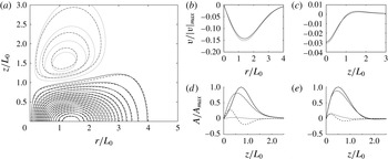
All the results we discussed above show that our linear model is able to predict, in a qualitative way, all the phenomenology arising from both experiments and numerical simulations. In this section we want to address this comparison in a more quantitative way. The good point about numerical simulations is that they allow us to look at each of the terms we neglected in the linear model and to compare them to the leading terms. In figure 13 we compare the results of the DNS S22 with the linear model. The radial and vertical cuts of the velocity field (b,c) show some discrepancies which can be estimated to be approximately 10 % with respect to the maximum. We then expect an error of the same order in predicting the value of the Rossby number. In (d,e) we report the absolute value of all the terms which appear in the density equation. The reason for considering only the density equation is that a systematic analysis of our numerical simulations showed that the ratio of the nonlinear terms to the leading terms is much less important in all other equations. One observe that at earlier time (d) the maximum of the nonlinear terms reaches 25 % of the leading terms while the ratio reduces to 15 % at larger time (e). Thus we verify that the linear model is a good approximation at any time.
Comparison of the DNS S22 with the linear model. On (a) we report the
 $(r,z)$
contour plot of the azimuthal velocity
 $v$
at time
 $t/T=1$
. Negative (positive) values are denoted by a solid (dash-dotted) line for the numerical simulation and by a dashed (dotted) line for the linear model. In (b,c) we report
 $v$
as a function of
 $r$
(b) at
 $z=0$
and
 $v$
as a function of
 $z$
(c) at the value of
 $r$
where
 $|v|$
is maximum. Velocity values are divided by velocity maximum at
 $t=0$
. In (d,e) we report the absolute value of all the terms which appear in the density equation as a function of
 $z$
at
 $r/L_{0}=0.1$
. (d)
 $t/T=0.1$
, (e)
 $t/T=1.0$
. —— time derivative, – – – nonlinear, – - – advection,
 $\cdots \cdots$
diffusion.

6 Conclusions
We study the evolution of an anticyclone created by injection in a laboratory rotating stratified flow. We measure the velocity field in the equatorial plane and observe a slow decay of the Rossby number. The profile of the azimuthal velocity spreads radially with a time scale of the order of
 $2/Ekf$
. The same behaviour is observed for different values of the ratio
 $N/f$
from 0.4 to 1.6, and the vortex always looks stable and axisymmetric within the range of explored parameters. We consider the axisymmetric Navier–Stokes equation in the Boussinesq approximation and linearize around the quasi-equilibrium solution. In the limit of small Rossby and Ekman numbers
 $|Ro|\ll 1$
,
 $Ek\ll 1$
, the system of equations reduces to a single equation for the pressure. We show that this equation ultimately reduces to a radial diffusion equation in the case
 $N_{f}=1$
; in this case the azimuthal velocity evolves in a self-similar way. For
 $N_{f}\neq 1$
a semi-analytic solution can be found using a spectral decomposition and solving the problem numerically. An integral solution for the Rossby number is presented, which is fast to compute and fairly consistent with our experimental results. We predict that the core of the azimuthal velocity perturbation should always spread radially irrespective of the initial aspect ratio. This validates the relevance of the time scale
 $T=2/fEk=L_{0}^{2}/\unicode[STIX]{x1D708}$
, even for small aspect ratios. This behaviour is validated by DNS (i.e. including all the nonlinear terms) and is in agreement with experimental results. We claim that this behaviour is a consequence of the main role played by the radial and vertical circulations
 $u$
and
 $w$
driven by viscous diffusion of the azimuthal velocity
 $v$
. Hence neglecting
 $u$
and
 $w$
may be misleading in determining the decay process, even if they are at least two orders of magnitude smaller than the azimuthal velocity
 $v$
. Beyond radial diffusion, we observe the appearance of new features in the azimuthal velocity field above and below the initial anticyclone. For
 $N_{f}>1$
, the azimuthal velocity diffuses also vertically and a column of weak negative vorticity is formed close to
 $r=0$
. For
 $N_{f}<1$
, a couple of weak cyclonic caps appear above and below the initial anticyclone. Finally, our theoretical analysis and numerical simulations show that the density diffusion comes into play as soon as
 $1/BuSc\sim 1$
, even if
 $Sc\gg 1$
, leading to significant vertical diffusion.
The present study was conceived as a completion of the previous work by Aubert et al. (Reference Aubert, Le Bars, Le Gal and Marcus2012) and Hassanzadeh et al. (Reference Hassanzadeh, Marcus and Le Gal2012), the aim being to determine the explicit time evolution of the relevant parameters
 $H,L,Ro$
and
 $N_{c}$
. The linear model we derive can be solved by a spectral method and allows us to predict the value of the velocity and density field at any time. The value of
 $H$
and
 $L$
are then deduced from a Gaussian fit while
 $Ro$
and
 $N_{c}$
correspond to the vertical and radial derivative at the origin of the velocity and density fields, respectively. The same approach is followed for DNS. We verify that in both cases the scaling law (1.1) is well satisfied.
As a conclusion we briefly address one of the natural phenomena which motivated the present study, i.e. the strikingly long lifetime of Meddies. The recent extensive review by Bashmachnikov et al. (Reference Bashmachnikov, Neves, Calheiros and Carton2015) reports that a large number of Meddies present a small Rossby number (
 $0.05<|Ro|<0.25$
) and a Burger number smaller than 0.5, which is also the case for our experiments. As a drawback, the experimental set-up does not allow us to reach ocean-relevant values of
 $N_{f}$
(e.g.
 $N_{f}\sim 30$
) by more than an order of magnitude. Nonetheless, the present study may serve as guideline for future field investigation and observations.
We verify that in our experiments the motor for the decaying process is viscosity, which is confirmed by our linear model and DNS. The comparison with real Meddies rises three major issues. Firstly, field observations (Richardson et al.
Reference Richardson, Bower and Zenk2000) showed that most Meddies are destroyed by collision with seamounts. Thus a viscous decay does not explain the very end of these objects, but still may describe their evolution for a significantly long time (
 $1{-}3~\text{yrs}$
). Then, our experimental anticyclones are more laminar than oceanic ones by orders of magnitudes. As a consequence, the flow at the boundaries of real Meddies is likely to be much more turbulent than what we observe in experiments and instabilities may appear which we did not observe. In particular the molecular viscosity
 $\unicode[STIX]{x1D708}$
of water seems not to be the relevant parameter for the definition of the Ekman number, thus we consider a turbulent effective viscosity
 $\unicode[STIX]{x1D708}_{eff}$
. The issues coming with this choice are twofold. First, the horizontal (
 $\unicode[STIX]{x1D708}_{eff}^{H}$
) and vertical (
 $\unicode[STIX]{x1D708}_{eff}^{V}$
) turbulent effective viscosities are likely not to be the same because the ocean is a stratified medium. Second, the values available in the literature for both
 $\unicode[STIX]{x1D708}_{eff}^{V}$
and
 $\unicode[STIX]{x1D708}_{eff}^{H}$
vary over quite a broad spectrum. At this stage we neglect this anisotropy by considering only one 3-D coefficient
 $\unicode[STIX]{x1D708}_{eff}=\unicode[STIX]{x1D708}_{eff}^{V}\sim 10^{-3}~\text{m}^{2}~\text{s}^{-1}$
, which is an intermediate value among those proposed in the literature (see e.g. Ledwell, Watson & Law Reference Ledwell, Watson and Law1993; Large & Gent Reference Large and Gent1999; Canuto et al.
Reference Canuto, Howard, Cheng and Dubovikov2001). The reason for this rough approximation is the following. The ratio of the vertical component of the Laplacian operator to the radial one can be estimated as
 $1/\unicode[STIX]{x1D6FC}^{2}\sim 2500$
, thus if
 $\unicode[STIX]{x1D708}_{eff}^{H}/\unicode[STIX]{x1D708}_{eff}^{V}$
is not too big, the horizontal contribution to the turbulent momentum dissipation (e.g.
 $\unicode[STIX]{x1D708}_{eff}^{H}\unicode[STIX]{x1D6FB}_{r}^{2}$
) remains negligible in any case. Bogucki, Jones & Carr (Reference Bogucki, Jones and Carr2005) performed in situ dye-release experiments which indicated a value of the horizontal eddy diffusivity of
 $\unicode[STIX]{x1D708}_{H}\sim 0.1~\text{m}^{2}~\text{s}^{-1}$
, consistent with the lower bound previously given by Sundermeyer & Ledwell (Reference Sundermeyer and Ledwell2001). According to that, and for
 $\unicode[STIX]{x1D708}_{eff}=10^{-3}~\text{m}^{2}~\text{s}^{-1}$
and
 $\unicode[STIX]{x1D6FC}\sim 0.02$
, our approximation appears to be consistent, even if a careful decision regarding its validity is beyond the scope of the present study. A similar question arises with the choice of the relevant salt diffusion coefficient (e.g. the choice of the effective Schmidt number) which is even more complex and beyond the scope of our study.
(a) The initial velocity field for our model Meddy, taken as Gaussian. We take
 $N_{f}=30$
,
 $\unicode[STIX]{x1D6FC}_{0}=0.017$
,
 $L_{0}=30~\text{km}$
,
 $Sc=30$
,
 $\unicode[STIX]{x1D708}_{eff}=10^{-3}~\text{m}^{2}~\text{s}^{-1}$
. (b,c) The velocity field after
 $3~\text{yrs}$
, in the case of plain diffusion and our model respectively. In (d) we report the evolution of the Rossby number in the case of plain diffusion (dashed line) and our model (solid line). At each time the velocity values are divided by the maximum of
 $|v|$
; contours are reported at a constant step of 0.05.

As an illustration of the application of the present paper, we show in figure 14 the predictions of our model in comparison with the simplified case where only the momentum dissipation is considered (e.g. both rotation and stratification are suppressed), choosing arbitrarily
 $H=500~\text{m}$
,
 $L=30~\text{km}$
,
 $\unicode[STIX]{x1D708}_{eff}=10^{-3}~\text{m}^{2}~\text{s}^{-1}$
and
 $Sc=30$
. We observe that, after
 $3~\text{yrs}$
, the velocity field tends towards a more isotropic configuration in the case of plain diffusion (second panel) while a smaller change is predicted by our model. In a similar way the modulus of the Rossby number decreases more slowly in the case of our model. Weak variations in the Rossby number have already been reported by the field studies of Armi et al. (Reference Armi, Hebert, Oakey, Price, Richardson, Rossby and Ruddick1989). Also we observe that the volume affected by a non-zero velocity
 $v$
and density anomaly
 $\unicode[STIX]{x1D70C}^{\prime }$
is not constant as already observed by Hebert, Oakey & Ruddick (Reference Hebert, Oakey and Ruddick1990). The volume delimited by any isoline of absolute density
 $\unicode[STIX]{x1D70C}$
does stay almost constant, which could be for example the envelope of the original amount of warm and salty water from the Mediterranean sea. However additional layers from the ambient fluid are entrained in anticyclonic rotation by viscosity and their absolute density is subsequently perturbed. The weak strength of the secondary circulations (i.e. relative to the rotation velocity) we observe can account only for the global stretching and not for strong intrusion mechanisms. On the contrary, field surveys on Meddy Sharon (Armi et al.
Reference Armi, Hebert, Oakey, Price, Richardson, Rossby and Ruddick1989) showed a net loss of salt and heat which was taken as the evidence of strong lateral intrusions. From this phenomenon Ruddick & Hebert (Reference Ruddick and Hebert1988) deduced the lateral turbulent diffusivity as
 $k_{H}\sim 0.4~\text{m}^{2}~\text{s}^{-1}$
, and an even higher estimation
 $k_{H}\sim 10~\text{m}^{2}~\text{s}^{-1}$
was given by Colin de Verdiere (Reference Colin de Verdiere1992). Finally, the mutual interaction of diffusion of heat, salt and momentum may be responsible for other instabilities such as double diffusion or McIntyre instability and will be the object of a future experimental work.
Summarizing, the final erosion of a Meddy may be controlled by mixing mechanisms other than the secondary circulations induced by momentum dissipation and inaccessible to our laminar experiments. Nevertheless the study we performed may explain why an object which is locally exposed to a viscous relaxation could show a surprisingly long lifetime as a result of a non-trivial mechanism acting at mesoscopic scales.
Acknowledgement
This work has been carried out thanks to the support of the A*MIDEX grant (ANR-11-IDEX-0001-02) funded by the French Government ‘Investissements d’Avenir’ program.