1. Introduction
In their experiments on explosions in coal mines, Mallard & Le Chatelier (Reference Mallard and Le Chatelier1883) reported for the first time the observation of the cellular nature of premixed flames. Since this pioneering work, many other experimental studies have confirmed this particular phenomenon (Smithells & Ingle Reference Smithells and Ingle1892; Groff Reference Groff1982; Bradley Reference Bradley1999). In two similar independent studies Darrieus (Reference Darrieus1938) and Landau (Reference Landau1944) proposed that the exothermic character of combustion is responsible for a hydrodynamic instability that leads to this corrugated pattern. By considering the front as a discontinuity between two inviscid flows of different densities and by using appropriate Rankine–Hugoniot conditions (see Landau & Lifshitz (Reference Landau and Lifshitz1959), chapter IX § 84), they performed a linear stability analysis and demonstrated that the front is unconditionally unstable, with a linearly increasing growth rate with respect to the wavenumber of the perturbation. By introducing a flame curvature dependence of the local flame speed, Markstein (Reference Markstein1951) managed to take flame thickness effects into account and obtained a dispersion relation for flames of finite thickness
 \begin{equation} \sigma=4\frac{\sigma_M}{k_c}\left(\left |k \right |-\frac{k^{2}}{k_c}\right), \end{equation}
where  $\sigma$ and
 $k$ are, respectively, the growth rate and the wavenumber of the perturbation,
 $\sigma _M$ is the growth rate of the most unstable wavelength and
 $k_c$ is a cutoff wavenumber. By introducing this new formalism and considering the gravity effect, Markstein reconciled the linear stability theory with experimental observations of downwards planar propagating flames (Quinard Reference Quinard1984; Searby & Quinard Reference Searby and Quinard1990). In particular, he pointed out that there is a small cutoff wavelength
 $\lambda _c=2{\rm \pi} /k_c$ due to thermal diffusion and a large cutoff wavelength caused by the stabilizing effect of gravity (Taylor Reference Taylor1950; Markstein Reference Markstein1951; Pelce & Clavin Reference Pelce and Clavin1982).
By looking at flames propagating in glass tubes, Markstein (Reference Markstein1949) also noted that the flame destabilization quickly leads to cellular patterns with stationary amplitude. As first identified by Karlovitz, Denniston & Wells (Reference Karlovitz, Denniston and Wells1951) and Manton, von Elbe & Lewis (Reference Manton, von Elbe and Lewis1952), this saturation has a nonlinear Huygens geometrical origin. Due to the normal propagation of the front, the radius of curvature increases (decreases) where the front is convex (concave) toward the unburned gases, leading to cells separated by abrupt cusps. Then, as a consequence of the flow induced in the unburned gas, this cellular pattern exhibits complex dynamics with larger cells growing at the expense of smaller neighbours in a way similar to bubbles competition in water (Layzer Reference Layzer1955). Numerical experiments either in the small expansion framework (Michelson & Sivashinsky Reference Michelson and Sivashinsky1977; Creta, Fogla & Matalon Reference Creta, Fogla and Matalon2011) or with a fully nonlinear model (Rastigejev & Matalon Reference Rastigejev and Matalon2006a; Creta & Matalon Reference Creta and Matalon2011; Altantzis et al. Reference Altantzis, Frouzakis, Tomboulides, Matalon and Boulouchos2012) have shown that these dynamics can lead to a final monocellular solution with characteristic sizes much larger than the most unstable wavelength  $\lambda _{max}=2\lambda _{c}$ predicted by the linear theory (Markstein Reference Markstein1949). These observations highlight the importance of the geometrical nonlinear effects in the long-time dynamics. Indeed, by forming a unique large cell stabilized by stretch (Uberoi Reference Uberoi1959), the hydrodynamic instability is responsible for a new stable state (Zeldovich et al. Reference Zeldovich, Istratov, Kidin and Librovich1980; Pelce & Clavin Reference Pelce and Clavin1987; Rabaud, Couder & Gerard Reference Rabaud, Couder and Gerard1988).
However, as observed in Markstein's experiments, for flames propagating in large vessels the merging process of cells is permanently supplied by the appearance of smaller cells (Michelson & Sivashinsky Reference Michelson and Sivashinsky1977; Gutman & Sivashinsky Reference Gutman and Sivashinsky1990; Rahibe et al. Reference Rahibe, Aubry, Sivashinsky and Lima1995; Rastigejev & Matalon Reference Rastigejev and Matalon2006a; Creta et al. Reference Creta, Fogla and Matalon2011; Altantzis et al. Reference Altantzis, Frouzakis, Tomboulides, Matalon and Boulouchos2012; Yu, Bai & Bychkov Reference Yu, Bai and Bychkov2015) created by splitting cells, after they reached an excessive size. This process never leads to the steady monocellular arrangement observed in smaller experiments (Uberoi Reference Uberoi1959; Von Lavante & Strehlow Reference Von Lavante and Strehlow1983; Pelcé-Savornin, Quinard & Searby Reference Pelcé-Savornin, Quinard and Searby1988). As first suggested by Joulin (Reference Joulin1989), these new crest formations are caused by the background noise that generates small wrinkles on the front that are in turn magnified by the Darrieus–Landau instability.
Hence, the dynamics of premixed flames results from the competition between several intrinsic properties (large-scale hydrodynamic coupling, thermodiffusive phenomena, geometrical nonlinear effects) and external stochastic forcing (hydrodynamics or thermal perturbations). Recently, by studying flames propagating in a Hele-Shaw burner, Almarcha et al. (Reference Almarcha, Radisson, Al Sarraf, Villermaux, Denet and Quinard2018) have shown that a small expansion model (Sivashinsky Reference Sivashinsky1977) provides a good description of the flame evolution both during the destabilization process and the long-time evolution. In particular, they demonstrated that the dynamics is accurately described by the trajectories of poles associated with the analytical solutions of the Michelson–Sivashinsky (MS) equation, up to a certain time. Beyond this time, the stochastic influence of the background noise becomes important and the system can no longer be described as a deterministic process. However, the pole-to-pole interaction still holds locally and allows us to predict some statistical properties of the flame front.
The aim of the present paper is to extend this previous work, in particular to characterize the typical time under which the flame dynamics remains deterministic, and to assess the validity of the statistical description at large time by comparing numerical, experimental and analytical results.
Compared to some of our recent papers, such as Al Sarraf et al. (Reference Al Sarraf, Almarcha, Quinard, Radisson and Denet2018a) and Almarcha et al. (Reference Almarcha, Radisson, Al Sarraf, Villermaux, Denet and Quinard2018), we have greatly improved the experimental techniques, which will allow us to study the repeatability of experiments and perform successful comparisons with theoretical results, both on the short-time nonlinear evolution and on the long-time statistical properties of the front.
The paper is organized as follows. In § 2 the experimental set-up used for this work is described, with special consideration given to its benefits and limitations. Then, early deterministic regimes of destabilization, nonlinear saturation and deterministic pole interaction are analysed in § 3 by way of the MS model whose relevance with regards to laboratory experiments is underlined. Finally, under the influence of stochastic external forcing, the statistical features of the flame topology are described in § 4.
2. Experimental set-up
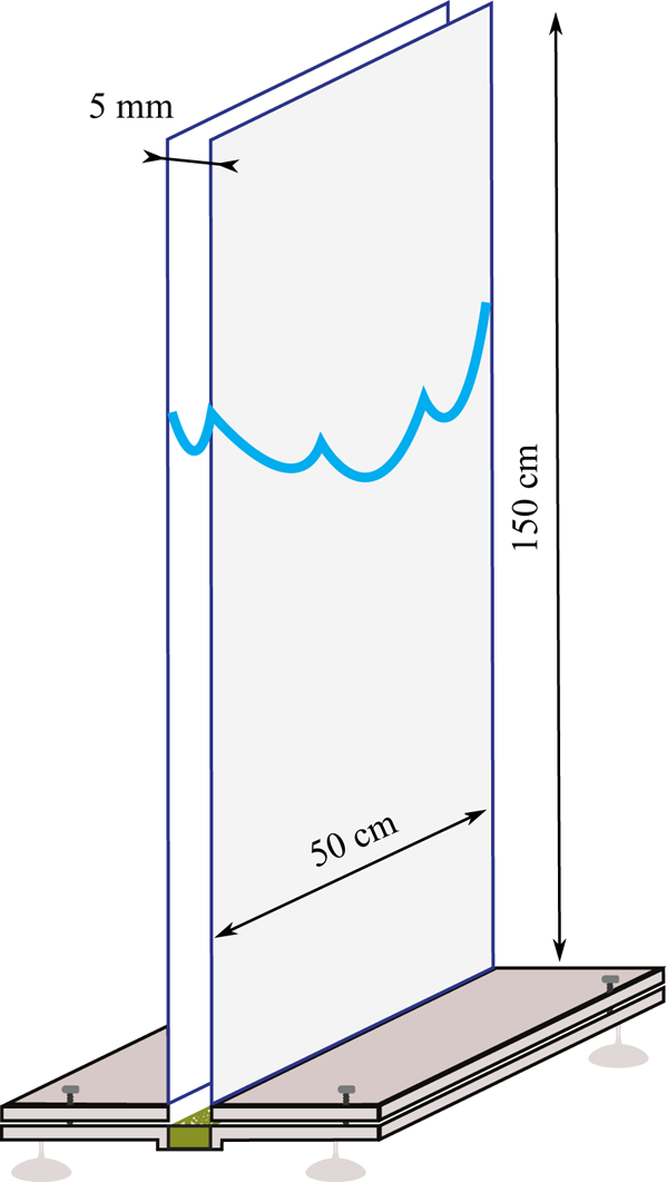
Most of the experimental studies about intrinsic flame instability and dynamics are based on anchored inverted V-flames (Truffaut & Searby Reference Truffaut and Searby1999) or flame propagation in expanding flame balls (Bradley Reference Bradley1999; Jomaas, Law & Bechtold Reference Jomaas, Law and Bechtold2007) or in glass tubes (Markstein Reference Markstein1949; Quinard Reference Quinard1984; Clanet & Searby Reference Clanet and Searby1998; Almarcha, Denet & Quinard Reference Almarcha, Denet and Quinard2015). In the first configuration, the angle between the front and the mean flow, implies the existence of a tangential velocity component. The wrinkles are advected along the front and the time over which their dynamics can be studied is limited. In the two other configurations, although long-time dynamics can be observed, the analysis of the front properties is difficult due to the three-dimensional character of the reaction sheet. In the present study, in order to avoid these shortcomings, the dynamics of the flame is analysed in a Hele-Shaw burner. The later was first proposed in the framework of an analytical study by Joulin & Sivashinsky (Reference Joulin and Sivashinsky1994) and introduced experimentally by Sharif, Abid & Ronney (Reference Sharif, Abid and Ronney1999). The apparatus consists of two vertically oriented borosilicate glass plates, 0.5 m wide and 1.5 m high, separated by a 5 mm gap, closed on the sides, open at the top and supplied with a premixed mixture at the bottom. The gap between the plates being of the order of the cutoff wavelength  $\lambda _c$ (depending on the equivalence ratio), this burner presents the major advantage of forcing the flame to be stationary in the thickness direction. Indeed, after a transient destabilization, the flame quickly moves toward a steady monocellular shape in the thickness direction. The dynamics is thus constrained in that direction and the analysis is significantly simplified into a bidimensional evolution. In the following sections we discuss in detail the choice of the main characteristics of this experimental apparatus.
2.1. Experimental procedure
For each experiment reported in the present study, the same operating procedure is used for each run. A flow of the combustible mixture, adjusted to the desired equivalence ratio ( $\varphi$) and dilution (
 $\delta =V_{O_2}/(V_{O_2}+V_{N_2}$)) with less than
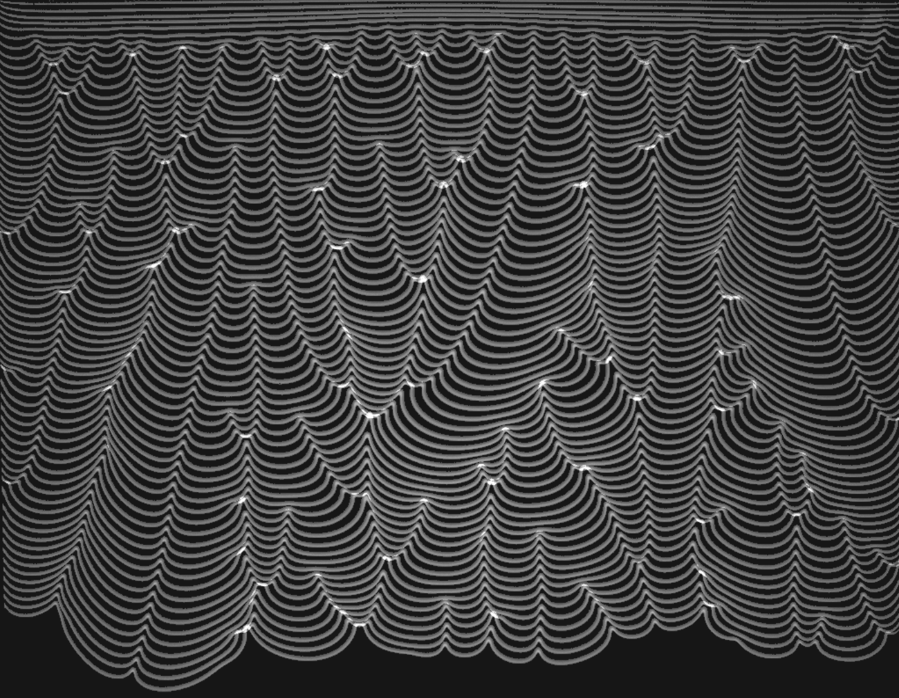
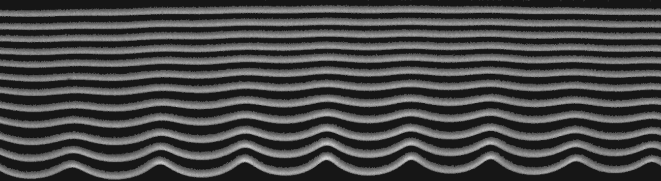
 $1\,\%$ error thanks to a PC-interface connected to Bronkhorst EL-Flow series mass-flow regulators, is maintained from bottom to top until there is complete homogenization in the burner. A two-dimensional inverted V-flame is ignited at the top of the burner and remains anchored as the flow rate exceeds the flame velocity, until the flow is stopped by closing a valve upstream. The flame then starts its downwards propagation (recorded using a high-speed camera), from an initially flat state that quickly leads to a cellular pattern due to hydrodynamic destabilizing effects (see figure 1).
Spatiotemporal diagram of a propane–air flame ( $\varphi =0.8$) propagating downwards in a Hele-Shaw burner. Field of view width is 46 cm. Time between two successive fronts is 14 ms. The front starts flat and is rapidly destabilized due to the Darrieus–Landau effect. Rapidly the instability is saturated by nonlinearities and a complex dynamics is observed. The crest merging and crest creations are readily visible.

2.2. Design of the burner
2.2.1. Thickness
The thickness of the burner is of prime importance. On one hand it must be thin enough to guarantee that the flame has a steady profile in the burner thickness direction. On the other hand, if the thickness is not large enough, momentum (Saffman & Taylor Reference Saffman and Taylor1958) and heat losses at the wall may completely modify the standard Darrieus–Landau picture. By measuring the flame propagation for stoichiometric propane–air flames in small channels (Gutkowski & Jarosiński Reference Gutkowski, Jarosiński, Jarosinski and Veyssiere2009) or in a Hele-Shaw burner (Jang, Jang & Kim Reference Jang, Jang and Kim2018), it has been shown that by decreasing channel width, the flame speed is first slightly increased up to a channel thickness around 5 mm due to surface incremental increase with curvature in the thickness. Then for smaller channel widths, as heat losses become dominant, the flame speed is strongly decreasing with the thickness of the burner until it reaches a quenching thickness ( $\approx$2 mm). For propane–air flames the 5 mm thickness seems to be a good compromise. This choice was confirmed in the same apparatus by the Al Sarraf et al. (Reference Al Sarraf, Almarcha, Quinard, Radisson and Denet2018a) growth rate measurements that follow the standard
 $\sigma \sim k-k^{2}$ (1.1) dispersion relation for all mixture compositions. The latter result shows that even if the heat and momentum losses due to the confinement of the flame may modify the coefficients in the dispersion relation, the underlying mechanisms governing the dynamics of the flame remain the same as for the three-dimensional configuration (Clanet & Searby Reference Clanet and Searby1998).
2.2.2. Width
The width of the cell has to be sufficiently large so that the side walls do not impact the flame behaviour in the middle of the cell. The mean size of the pattern expected in the late-time dynamics is approximately a few times (Cambray, Joulain & Joulin Reference Cambray, Joulain and Joulin1994) the maximum unstable wavelength (approximately 1 cm here). In order to get a sufficient number of cells for the late-time regime studied in § 4, we use a burner 10 times larger than this mean cell size, i.e. 50 cm wide (figure 2).
Sketch of the experimental apparatus used in this study. The two glass plates are vertically oriented and separated by a thin gap closed on the sides and at the bottom. The burner is filled with an homogeneous mixture of propane and air at desired equivalence ratio  $\varphi$ and dilution
 $\delta$ (see § 2.1 for definition). The flame is ignited at the top and propagates downwards.

2.2.3. Height
As the flame propagates from top to bottom, the height of the burner imposes the time over which the flame propagation can be studied. As we are interested in both the short- and long-time dynamics, the apparatus should be high enough to guarantee that the flame reaches a fully developed stage. Due to nonlinear interaction, this time can be significantly longer than the characteristic time of the instability  $t_{\sigma }=1/\sigma _{max}$ (Joulin & Cambray Reference Joulin and Cambray1992). Considering a typical
 $t_{\sigma }\sim 10^{-2}$ s (Al Sarraf et al. Reference Al Sarraf, Almarcha, Quinard, Radisson and Denet2018a) and a typical flame propagation speed
 $u_T\sim 1\ \textrm {m}\ \textrm {s}^{-1}$, the time for the flame to propagate from top to bottom of the 1.5 m high burner, is of the order
 ${\sim }10^{2}t_\sigma$.
2.2.4. Valve closure system
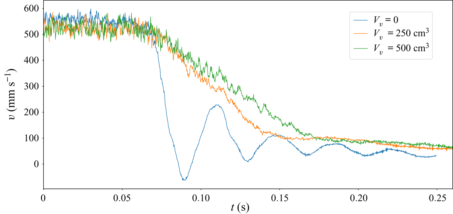
The short-time destabilization is likely to be altered by the gas deceleration after closing the valve. The closure system must be carefully designed to avoid undesirable buoyancy effects including Rayleigh–Taylor instability (Taylor Reference Taylor1950). In order to characterize the acceleration experienced by the gas after the valve closure, we measure the evolution of the flow speed by using particle image velocimetry. For this purpose, a continuous 532 nm laser sheet is placed in the Hele-Shaw burner and the mixture flow is seeded with oil droplets. We perform repeatable experiments using a solenoid valve (contrary to the Al Sarraf et al. (Reference Al Sarraf, Almarcha, Quinard, Radisson and Denet2018a) study where the flow was stopped manually). When the valve is closed, it triggers a high-speed camera that records the flow deceleration. The velocity field is then obtained by a particle image velocimetry cross-correlation algorithm (Meunier & Leweke Reference Meunier and Leweke2003). The vertical velocity of the flow is measured at one point at the top of the burner, a few centimetres inside. A vessel (of volume  $V_v$) can be placed between the valve and the burner, in order to modify the decay rate of the flow. The evolution of the vertical velocity is plotted in figure 3 for three different values of
 $V_v$. As can be seen, when
 $V_v=0$, the system behaves as an underdamped oscillator (see figure 3 (blue curve)) and the flame experiences strong acceleration effects (
 ${\simeq }4g$) which are not desirable for an intrinsic flame dynamics analysis. The underlying mechanism for these oscillations is beyond the scope of the present paper and was studied in a recent paper (Radisson, Piketty-Moine & Almarcha Reference Radisson, Piketty-Moine and Almarcha2019). However, to avoid these shortcomings, for all the experiments reported hereafter, a vessel
 $V_v=250\ \textrm {cm}^{3}$ is placed between the valve and the burner. In this way, the measured deceleration of the flow is approximately half the magnitude of gravity (see figure 3 (orange curve)), ensuring that Rayleigh–Taylor effects are negligible.
Evolution of the vertical speed of the flow after the valve closure for three different set-ups. After a delay time (0.7 s) corresponding to the closure time of the solenoid valve, the deceleration of the flow is observed.

2.3. Flammability limits
The propane–air mixture was varied in order to explore the full range of equivalence ratios, up to the flammability limits of the apparatus, that allow the propagation of a flame. For the burner at ambient temperature  ${\approx }293$ K the flammability limits were found to be approximately
 $\varphi \approx 0.65$ on the lean side and
 $\varphi \approx 1.5$ on the rich side. The present work is limited to a range of equivalence ratios far from these extinction limits (
 $0.8<\varphi <1.3$).
2.4. Data acquisition
The flame dynamics are analysed by recording flame chemiluminescence images with a 8-bit high-speed video camera (Photron FASTCAM MINI AX 200) (figure 1). The flame-front coordinates are then extracted from these images by way of Python image processing (open-source library Scikit-Image) with subpixel accuracy.
3. Deterministic dynamics
In figure 1, two typical stages are clearly visible. Starting from an initially flat flame, some wrinkles first emerge and grow to form crests with saturated amplitude. In a second stage, these crests evolve in a complex motion including crest merging and new crest creations. In this section, we analyse the linear stage and then compare the evolution of the front with a nonlinear model and its analytical solutions. We also evaluate the time during which the trajectories of crests are deterministic.
3.1. Growth rate measurements
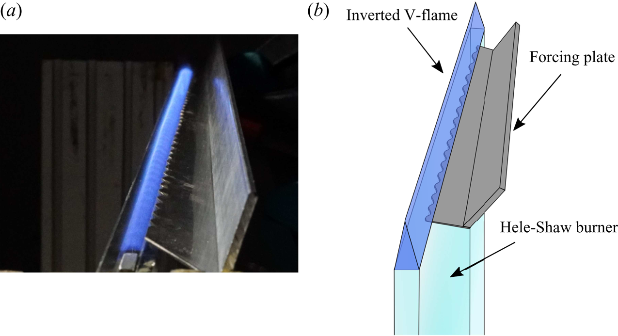
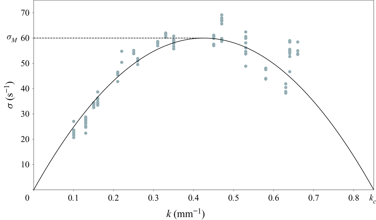
The unstable nature of flames is unveiled by the linear destabilization, starting from an initially flat flame. This is easily obtained in our experiment as the flame is anchored on the straight upper edge of the cell (figure 4) before it starts entering the cell. In that case, the most unstable wavelength emerges. However, in order to access the dispersion relation and the key features exposed on (1.1), it is necessary to start from an initial condition (figure 5) forced to develop selected wavelengths by using the forcing method introduced in Al Sarraf et al. (Reference Al Sarraf, Almarcha, Quinard, Radisson and Denet2018a). This procedure allows us to measure the growth rate of distinct wavelengths. Contrary to the Al Sarraf et al. (Reference Al Sarraf, Almarcha, Quinard, Radisson and Denet2018a) study, the burner supply line is now equipped with a solenoid valve which allows us to perform experiments in a repeatable way and the forcing plates are more accurately machined (we use for measuring growth rates a sinusoidal profile obtained by laser cutting). These improvements of experimental techniques allow us to present a new extended set of growth rate measurements and particularly to obtain a more precise value of the cutoff wavenumber. This better confidence on the  $k_c$ value will be of particular importance for the results presented in the next sections. The data obtained from these measurements are shown in figure 6. The theoretical dispersion relation (1.1) is then fitted with
 $\sigma _M$, the growth rate of the most unstable wavelength, and
 $k_c$, the cutoff wavenumber. As predicted by Sivashinsky (Reference Sivashinsky1977), we will show that the overall dynamics observed in our experiments can be described knowing these two parameter values.
Sketch of the experimental set-up used to perform growth rate measurements.

Unstable mode growth record in the first instants of propagation after stopping the flow (field of view 158 mm). Propane–air flame  $\varphi =0.8$. (Fronts have been artificially shifted to distinguish each time of evolution. Time between each front
 $dt=7.5$ ms.) Here the flame is initially forced with a 18 mm wavelength. See Al Sarraf et al. (Reference Al Sarraf, Almarcha, Quinard, Radisson and Denet2018a) for details about forcing methods.

Growth rate measurements (downwards propagating propane–air flame  $\varphi =0.8$) obtained from flame dynamics analysis in the first instants of propagation. The experimental points are then fitted with the theoretical dispersion relation in order to determine the relevant
 $\sigma _M$ and
 $k_c$ parameters for our experiments.

3.2. Saturation
As evidenced by the flame-front evolution in figure 5, the exponential growth is rapidly saturated by a geometrical effect: the normal propagation of the front. This nonlinear effect is responsible for the formation of crests that limit the wrinkles’ amplitude. Therefore, a relevant investigation of the physical mechanisms involved in the long-time dynamics requires nonlinear analysis with all the basic ingredients highlighted before: large-scale hydrodynamic instability, thermal restabilization at short wavelength and nonlinear geometrical effects able to saturate the instability. Carrying these three essential basic features and possessing the obvious advantage of being analytically tractable, the MS equation (Sivashinsky Reference Sivashinsky1977) seems to be an ideal candidate to allow a detailed description of the flame dynamics. In the following section, the model and its analytical solutions are first introduced and their essential properties are recalled. Its relevance regarding the experiments is then demonstrated.
3.3. An asymptotic model: the MS equation
Considering an infinitesimal thickness flame separating two inviscid flows of different densities and a kinematic relation with a linear dependence on flame-front curvature for the local flame speed, Sivashinsky (Reference Sivashinsky1977) showed that it is possible to obtain an evolution equation for the flame front. By performing an asymptotic development of the full set of equations in the limit of small expansion parameter  $\gamma \rightarrow 0$ (
 $\gamma =(\rho _u-\rho _b)/\rho _u$), the flame-front dynamics is reduced to a pseudodifferential equation governing the motion of the front. At first order in
 $\gamma$ it takes the form
 \begin{equation} \phi_t+\frac{u_A}{2}\phi_x^{2}=\frac{4\sigma_M}{k_c}\left(\frac{\phi_{xx}}{k_c}+ I(\phi, x)\right), \end{equation}
where  $\phi$ stands for the vertical position of the front,
 $x$ is the transverse coordinate and
 $t$ the time. Here,
 $\sigma _M$ and
 $u_A$ are parameters depending on the laminar flame speed and the expansion parameter
 $\gamma$. Here,
 $k_c$ is the cutoff wavenumber depending on the reactive mixture properties and
 $I(\phi ,x)$ is a linear operator given by
 \begin{equation} I(\phi, x)=\int_{-\infty}^{\infty}\left|k\right|\textrm{e}^{\textrm{i}kx}\hat{\phi}(k, t)\, \textrm{d} k. \end{equation}
As can be seen in (3.1), from the first order in  $\gamma$, the Sivashinsky model contains the three essential basic ingredients listed before. Moreover, it was shown later that despite new terms correcting the mean front displacement, this equation keeps almost the same functional structure up to second order (Sivashinsky & Clavin Reference Sivashinsky and Clavin1987; Joulin & Cambray Reference Joulin and Cambray1992) and third order in
 $\gamma$ (Kazakov Reference Kazakov2005a,b Reference Kazakov) (stationary case). In (3.1), the last term is the instability term. Due to multiplication by
 $|k|$ in Fourier space, the
 $I(\phi , x)$ is responsible for the amplification of any disturbance with a linearly increasing growth rate with
 $k$ the wavenumber of the perturbation. The curvature term
 $\phi _{xx}$ comes from the thermal diffusive restabilization and is responsible for the damping of disturbances at small scale. Finally, the
 $\phi _x^{2}$ is a slope advection term and is responsible for the formation of cusps due to normal propagation of the front. In a way similar to the dynamics described by the Burgers equation, the cusps are regularized by the diffusive term in the right-hand side. These dynamics never lead to real slope singularity but to the formation of abrupt crests with rounded tips as can be seen in late stages of figure 5. As first shown by Bessis & Fournier (Reference Bessis and Fournier1984), these quasi-cusps can be expressed in term of complex singularities appearing in complex-conjugate pairs. Accordingly, the MS model admits analytical solutions which allow us to express the evolution of the flame front in terms of the trajectories of these complex singularities.
3.4. Analytical pole solutions for the Sivashinsky equation
As first noted by Thual, Frisch & Hénon (Reference Thual, Frisch and Hénon1985), the MS model belongs to a broader class of nonlinear models (Lee & Chen Reference Lee and Chen1982) which admit analytical solutions in the form of complex pole decomposition: the solutions of (3.1) (with periodic boundary conditions) can be expressed as
 \begin{equation} \phi(x, t)=-\frac{8\sigma_M}{u_Ak_c^{2}}\sum_{n=1}^{2N} \ln\left(\sin\left(\frac{{\rm \pi}\left(x-z_n(t)\right)}{\Lambda}\right)\right),\end{equation}
where  $\Lambda$ is the width of the domain,
 $N$ is the number of complex conjugate pole pairs involved in the solution and
 $z_n$ are the positions of the poles in the complex plane. Roughly speaking, each pair of poles is responsible for a distortion of the front around the abscissa
 $x= \textrm {Re}(z_n)$. The distortion is even more pronounced as
 $\textrm {Im}(z_n)$ is small (
 $\phi _x\rightarrow \pm \infty$ when
 $\textrm {Im}(z_n) \rightarrow 0$).
Substituting (3.3) in (3.1), the problem of the front dynamics is reduced to a dynamical system of  $2N$ ordinary differential equations, that govern the poles trajectories in the complex plane,
 \begin{equation} \dot{z}_n=\frac{4\sigma_M}{k_c}\left[\frac{2{\rm \pi}}{\Lambda k_c}\sum_{p \neq n}\cot \left(\frac{\rm \pi}{\Lambda}\left(z_p-z_n\right)\right)-\textrm{i}\,sign\left( \textrm{Im}(z_n)\right)\right],\end{equation}
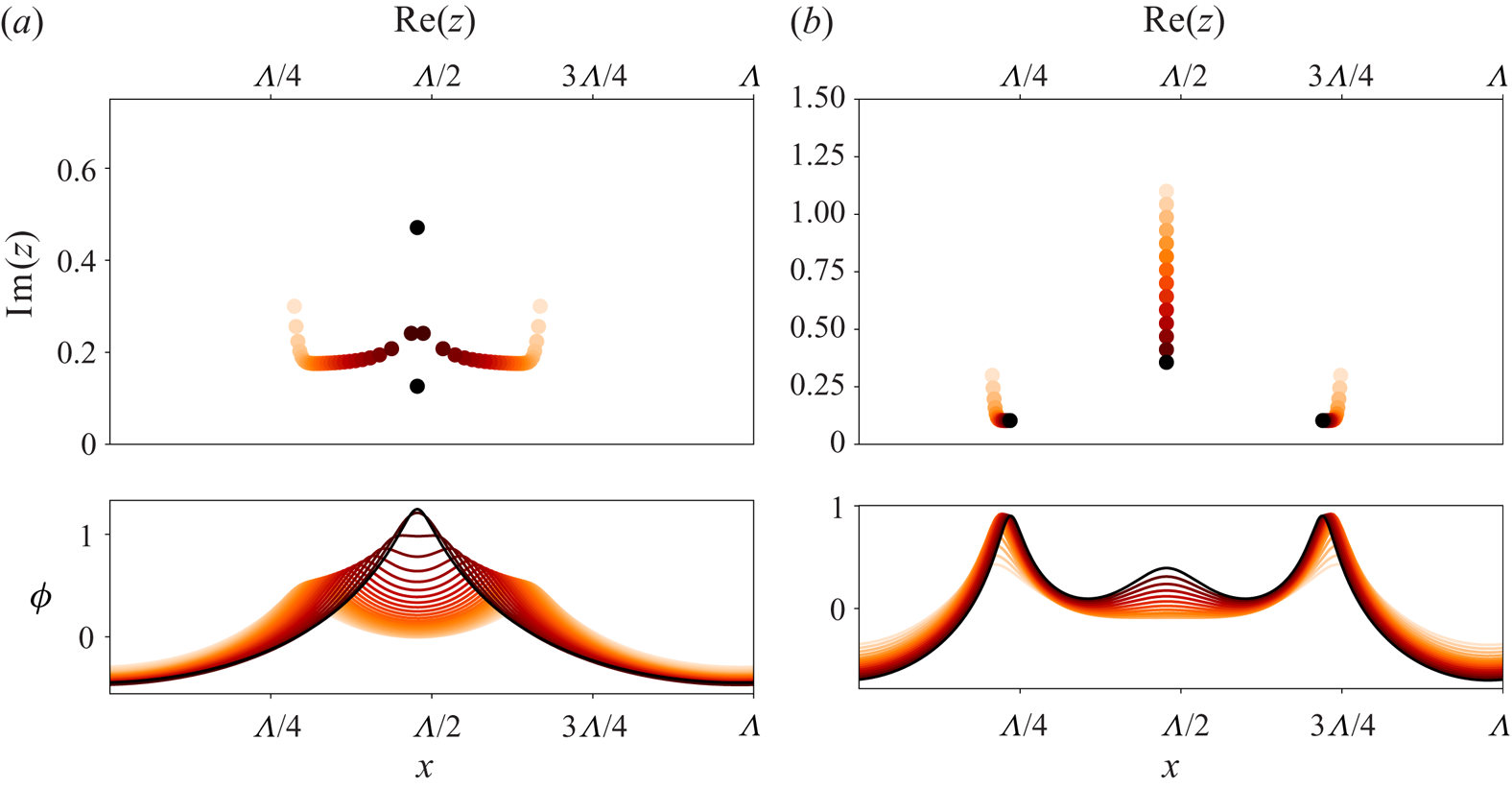
where the first term in brackets is responsible for an attractive interaction between poles along the real axis, and a repulsive one along the imaginary axis. As each crest is the manifestation of at least one pair of poles in the complex plane, this horizontal attraction between poles is responsible for the crest merging observed in our experiments (see figure 1). Due to vertical repulsion, when two pairs of poles tend toward the same abscissa, each of them follows an hyperbolic trajectory (Thual et al. Reference Thual, Frisch and Hénon1985) in the complex plane and poles tend to align vertically forming giant crests (see the left part of figure 7). This pole dynamics leads to a steady giant cusp solution (the monocellular arrangement previously quoted) with all the poles aligned along the imaginary axis (Thual et al. Reference Thual, Frisch and Hénon1985). This process is similar to the pole condensation in the Burgers equation and may be viewed as the mechanism leading to shock coalescence (see Bessis & Fournier Reference Bessis and Fournier1984). In order to test the MS model and the accuracy of the pole solutions, we analyse the dynamics of a two cusps merging.
Evolution of arbitrary set of poles according to (3.4) and their corresponding solutions for the flame front (the time goes from the light initial condition to the dark final one). (a) Merging of two crests due to pole attraction along the real axis. (b) New crest creation due to attraction of a pole initially far from the real axis.

3.5. Crest merging
As in Almarcha et al. (Reference Almarcha, Radisson, Al Sarraf, Villermaux, Denet and Quinard2018), we are interested in the mechanism of cell fusion. We first present a formal derivation of the analytic law for cusp aggregation.
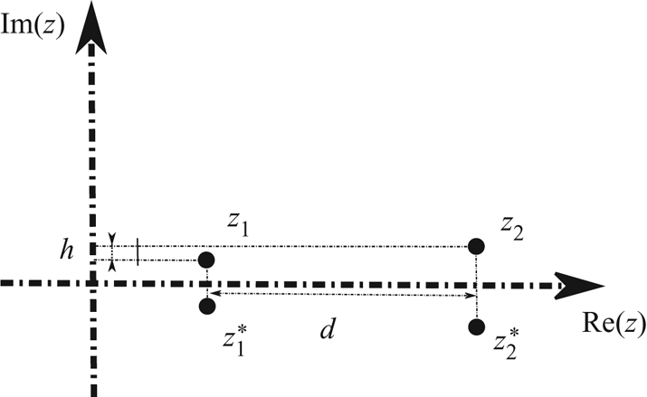
We consider two pairs of complex conjugate poles 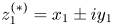 $z_1^{(*)}=x_1\pm iy_1$ and
 $z_2^{(*)}=x_2\pm iy_2$ sufficiently close to each other so that we can ignore their interaction with other poles (see figure 8). According to (3.4) and giving
 $C_1={4\sigma _M}/{kc}$ and
 $C_2={2{\rm \pi} }/{\Lambda k_c}$, we have
 \begin{equation} \Rightarrow \left\{\begin{array}{@{}l} \dot{z}_1=\displaystyle C_1\left\{C_2\left[\cot\left(\dfrac{\rm \pi}{\Lambda}\left(d+\textrm{i}h\right)\right)+ \cot\left(\dfrac{\rm \pi}{\Lambda}\left(d-\textrm{i}l\right)\right)+\cot\left(-2\textrm{i}\dfrac{\rm \pi}{\Lambda}y_1\right)\right]-\textrm{i}\right\},\\ \dot{z}_2=\displaystyle C_1\left\{C_2\left[\cot\left(-\dfrac{\rm \pi}{\Lambda}(d+\textrm{i}h)\right)+ \cot\left(-\dfrac{\rm \pi}{\Lambda}(d+\textrm{i}l)\right)+\cot\left(-2\textrm{i}\dfrac{\rm \pi}{\Lambda}y_2\right)\right]-\textrm{i}\right\},\\ \dot{z}_1^{*}=\displaystyle C_1\left\{C_2\left[\cot\left(\dfrac{\rm \pi}{\Lambda}\left(d+\textrm{i}l\right)\right)+ \cot\left(\dfrac{\rm \pi}{\Lambda}\left(d-\textrm{i}h\right)\right)+\cot\left(2\textrm{i}\dfrac{\rm \pi}{\Lambda}y_1\right)\right]+\textrm{i}\right\},\\ \dot{z}_2^{*}=\displaystyle C_1\left\{C_2\left[\cot\left(-\dfrac{\rm \pi}{\Lambda}(d-\textrm{i}l)\right)+ \cot\left(-\dfrac{\rm \pi}{\Lambda}(d-\textrm{i}h)\right)+\cot\left(2\textrm{i}\dfrac{\rm \pi}{\Lambda}y_2\right)\right]+\textrm{i}\right\}, \end{array}\right. \end{equation}
Interaction between two pairs of poles, sufficiently close to each other so that we can ignore interaction with other poles, but sufficiently far to have  $h \ll d$ in order to consider a two-body interaction with a double charge (see (3.5)).

with
 \begin{equation} \left.\begin{array}{l@{}} d=x_2-x_1,\\ h=y_2-y_1,\\ l=y_2+y_1, \end{array}\right\}\end{equation}
so that
 \begin{align} \Rightarrow \dot{d} &= -C_1C_2\left\{\cot\left(\frac{\rm \pi}{\Lambda}\left(d+\textrm{i}h\right)\right)+ \cot\left(\frac{\rm \pi}{\Lambda}\left(d-\textrm{i}h\right)\right) \right. \nonumber\\ &\quad \left.+\cot\left(\frac{\rm \pi}{\Lambda}\left(d-\textrm{i}l\right)\right)+ \cot\left(\frac{\rm \pi}{\Lambda}\left(d+\textrm{i}l\right)\right)\right\}. \end{align}
In the limit where poles are sufficiently close to each other so that we can ignore interaction with other poles, and where the two poles are near their equilibrium position along the imaginary axis (i.e. attraction due to second term in the right-hand side of (3.4) in equilibrium with the repulsive force due to interaction with their c.c  $\Rightarrow h\ll \Lambda /{\rm \pi}$ and
 $l\ll \Lambda /{\rm \pi}$)
 \begin{equation} \Rightarrow \dot{d}=-\frac{2 \Lambda C_1C_2}{{\rm \pi} d\left(1+\left(\frac{h}{d}\right)^{2}\right)}- \frac{2 \Lambda C_1C_2}{{\rm \pi} d\left(1+\left(\frac{l}{d}\right)^{2}\right)}, \end{equation}
which yields, at leading order when  $h/d \rightarrow 0$ and
 $l/d \rightarrow 0$, to
 \begin{equation} \Rightarrow d^{2}(t)=d_0^{2}-\frac{8 C_1 C_2 \Lambda}{\rm \pi}t=d_0^{2}-\frac{64\sigma_M}{k_c^{2}}t. \end{equation}
The latter is equivalent to the interaction between two poles on the real axis, each of them having a double charge.
As each pole  $z$ is responsible for the presence of a crest at
 $x= \textrm {Re}(z)$, the squared distance between two crests is a linearly decreasing function of
 $t$ with a slope
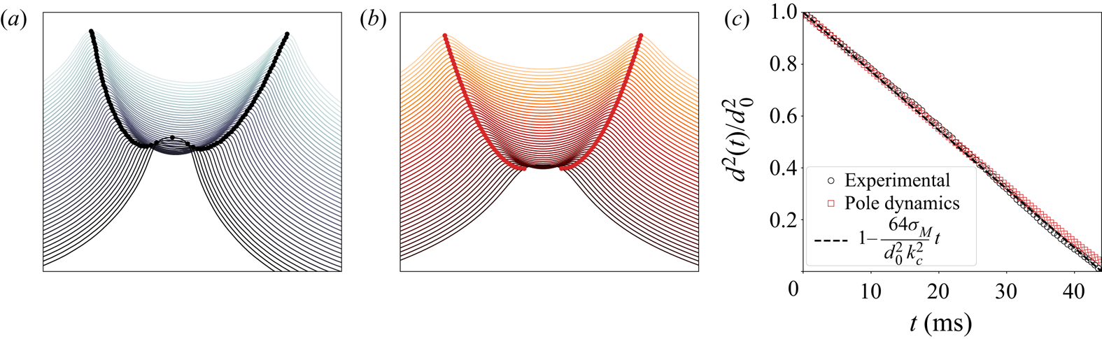
 $d^{2}_t=-64\sigma _M/k_c^{2}$. This theoretical law, already introduced by Almarcha et al. (Reference Almarcha, Radisson, Al Sarraf, Villermaux, Denet and Quinard2018) is now checked experimentally and numerically.
For this purpose, the pole dynamics ordinary differential equation (3.4) is integrated from an initial condition with two isolated poles with equal imaginary parts ( $\textrm {Im}(z_1)= \textrm {Im}(z_2$)) (figure 9b). The evolution of the horizontal distance between the two poles (
 $d(t)= \textrm {Re}(z_2)- \textrm {Re}(z_1$)) is computed. On the other hand, an experimental merging of two isolated crests is analysed in the Hele-Shaw burner (figure 9a), and the evolution of the distance between them
 $d(t)=\sqrt {(x_r-x_l)^{2}+(y_r-y_l)^{2}}$ is computed. These two evolutions are then compared with the asymptotic law (3.9) using
 $\sigma _M$ and
 $k_c$ values obtained in § 3.1 (see right part of figure 9). As can be seen, the experiment not only corroborates the functional form of (3.9) but also the value of the slope, which was not obtained in Almarcha et al. (Reference Almarcha, Radisson, Al Sarraf, Villermaux, Denet and Quinard2018), due to a low precision on the cutoff wavenumber. This good agreement underlines the relevance of pole description for real flames.
Merging process between two isolated crests of a propane–air flame ( $\varphi =0.8$). (a) Successive fronts extracted from an experimental movie during the merging process. Time between two successive fronts
 $dt=2$ ms. (b) Flame-front evolution given by pole dynamics starting from two isolated pairs of poles. Time between two successive fronts
 $dt=2$ ms. (c) Evolution of the squared non-dimensional distance between the two crests in the course of time. The evolution observed on experimental flame (black circles) is compared with the one given by pole dynamics given by (3.4) (red squares) and to the theoretical law (3.9) (dashed line). Here, the
 $\sigma _M$ and
 $k_c$ values are those obtained in § 3.1.

3.6. Crest creation
In viscous Burgers dynamics, shocks are relaxed by pole repulsion to  $\pm \textrm {i}\infty$. In MS dynamics, instead, the second term in brackets in (3.4), is responsible for an attraction of poles toward the real axis. Due to this instability term, poles that are initially far from the real axis (therefore not visible on the front solution) may drift toward the real axis. This mechanism can be responsible for the appearance of new crests (see the right part of figure 7). However, in our experiments we observe permanent new crest creation during the flame propagation (see figure 1), which could be seen as the presence of an infinite (
 $N\to \infty$) reservoir of poles initially far from the real axis. On the other hand if
 $N$ is finite, the pole dynamics cannot describe the experimental observations for large times. The problem of new crest creations is therefore of fundamental importance to settle whether our experiments can be described by a purely deterministic model such (3.4). To make the discussion about new crest creations simpler (and simplify the comparison between the numerical experiments in § 4.1.1 and the other ones from the literature), we introduce the non-dimensional MS equation. Introducing
 $\Lambda =2{\rm \pi} /K$ the width of the domain considered and setting the following appropriate non-dimensional variables
 \begin{equation} \left.\begin{array}{c@{}} \tau=\displaystyle{\dfrac{8{\rm \pi}\sigma_M}{\Lambda k_c}}t,\\ X=\displaystyle{\dfrac{2{\rm \pi}}{\Lambda}}x,\\ \Phi=\displaystyle{\dfrac{u_A k_c{\rm \pi}}{2\Lambda \sigma_M}}\phi. \end{array}\right\}\end{equation}
Equation (3.1) is reduced to a one parameter equation
 \begin{equation} \Phi_{\tau}+\tfrac{1}{2}\Phi_X^{2}=\nu \Phi_{XX}+ I\left(\Phi, X\right),\end{equation}
where the control parameter  $1/\nu =k_c/K$ corresponds to the ratio of the width of the domain to the shortest unstable wavelength. Commonly called the unstable modes number, this parameter stands for the only non-dimensional number governing the flame dynamics. Indeed, both experimental studies (Markstein Reference Markstein1949; Istratov & Librovich Reference Istratov and Librovich1969; Groff Reference Groff1982; Gostintsev, Istratov & Shulenin Reference Gostintsev, Istratov and Shulenin1989; Jomaas et al. Reference Jomaas, Law and Bechtold2007), and numerical experiments, either in the MS framework (Michelson & Sivashinsky Reference Michelson and Sivashinsky1982; Thual et al. Reference Thual, Frisch and Hénon1985; Gutman & Sivashinsky Reference Gutman and Sivashinsky1990; Filyand, Sivashinsky & Frankel Reference Filyand, Sivashinsky and Frankel1994; Joulin & Sivashinsky Reference Joulin and Sivashinsky1994), or using a fully nonlinear model (Rastigejev & Matalon Reference Rastigejev and Matalon2006a), or direct numerical simulation (Yu et al. Reference Yu, Bai and Bychkov2015), have reported a strongly dependent dynamics on this
 $1/\nu$ parameter. For small domains (large
 $\nu$), (considering periodic boundary conditions) the dynamics always leads to a steady single crest configuration (sometimes double crest configuration for Neumann boundary conditions) whereas for larger domains, as the cells become wider, one can observe secondary wrinkles permanently appearing on the primary structures. This behaviour is in contrast with the dynamics described by (3.4), which always leads to a steady state, whatever the size of the domain (Thual et al. Reference Thual, Frisch and Hénon1985; Joulin & Sivashinsky Reference Joulin and Sivashinsky1994; Rahibe et al. Reference Rahibe, Aubry, Sivashinsky and Lima1995). The differences observed between the dynamics described by (3.1) and the one described by (3.4) for large domains, is indeed quite surprising. As first proposed by Joulin (Reference Joulin1989), the new crest creations actually depend on the background noise (numerical noise, flow perturbations). Indeed, as first shown by Thual et al. (Reference Thual, Frisch and Hénon1985), the steady monocoalescent solution is the strongest attractor of (3.4) and any initial condition tends to this
 $N_{opt}$ poles pile solution (Thual–Frisch–Hénon (TFH) solution). This solution is such that
 $2N_{opt}-1<1/\nu <2N_{opt}+1$ (where
 $N_{opt}$ is called the optimal pole number), extra poles are repealed to infinity. However, even if the TFH solution is the only stable one for both (3.1) and (3.4) (Vaynblat & Matalon Reference Vaynblat and Matalon2000a,b Reference Vaynblat and Matalon), the number of equilibrium solutions is growing faster than linearly with
 $1/\nu$, leading rapidly to a large number of solutions (Denet Reference Denet2006). The external noise, which is responsible for the permanent addition of new poles (Joulin Reference Joulin1988; Kupervasser, Olami & Procaccia Reference Kupervasser, Olami and Procaccia1996; Olami et al. Reference Olami, Galanti, Kupervasser and Procaccia1997), may cause the system to permanently jump from one solution to another if poles are introduced close enough to the real axis (Denet Reference Denet2006). Moreover, this unsteady behaviour can be explained without invoking nonlinear mechanisms, because of the existence of transient growth phenomena (Karlin Reference Karlin2002, Reference Karlin2004) not taken into account in the modal analysis carried out by Vaynblat & Matalon (Reference Vaynblat and Matalon2000a) and making the TFH solution an unstable equilibrium for (3.1). To be physically relevant for large-scale flames, it is thus necessary to add a stochastic forcing term in (3.1) to mimic the noise experienced by the flame front (Cambray & Joulin Reference Cambray and Joulin1992; Cambray et al. Reference Cambray, Joulain and Joulin1994; Creta et al. Reference Creta, Fogla and Matalon2011). From the pole decomposition standpoint, as said before, the external perturbations act as a stochastic source of new poles (Joulin Reference Joulin1988; Kupervasser et al. Reference Kupervasser, Olami and Procaccia1996; Olami et al. Reference Olami, Galanti, Kupervasser and Procaccia1997). But until now the new poles are introduced in a completely artificial manner, and how to determine the probability function of adding a new pole at a certain location in the complex plane remains an open question. Despite this effect, in the following section we will show that the flame propagation observed in our experiments can be treated as a deterministic process for some time of evolution, and that the dynamics described by (3.4) is then experimentally relevant.
3.7. Initial forced pole solution
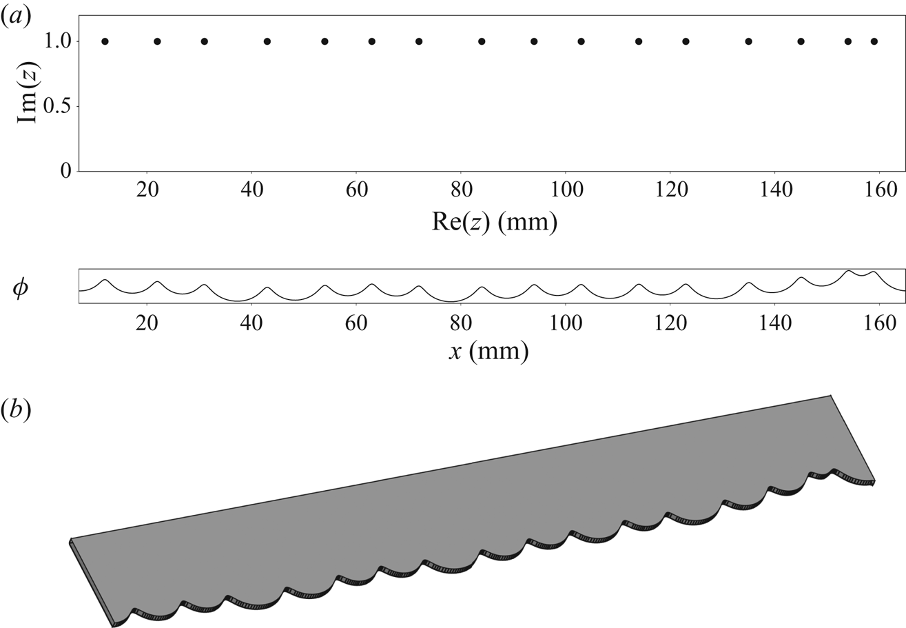
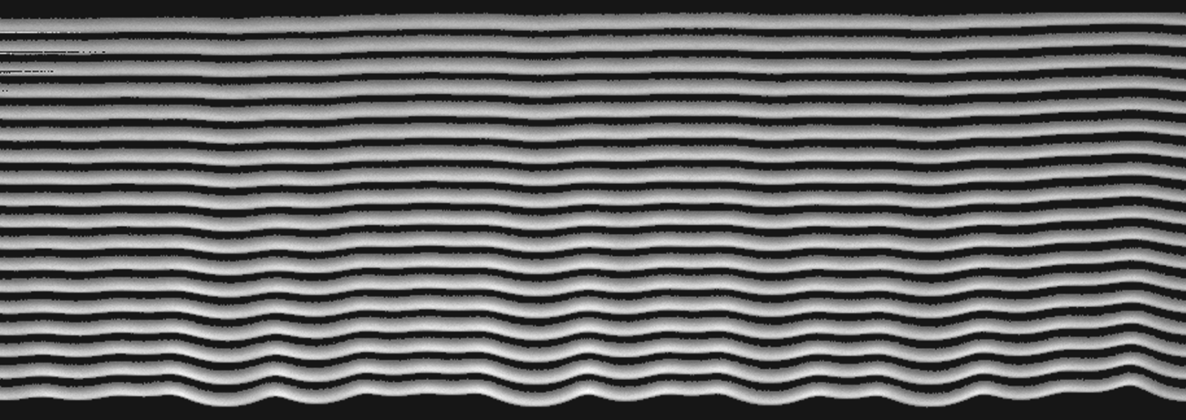
In a recent paper (Almarcha et al. Reference Almarcha, Radisson, Al Sarraf, Villermaux, Denet and Quinard2018), by being able to fit the (3.3) solution on a front extracted from experiments with a small number of poles, we have already shown that pole solutions can be relevant regarding real flames. The present section is another step forward and comes with the aim of characterizing the repeatability of the experiments in order to extract a typical time beyond which the flame dynamics can no longer be described as a purely deterministic pole dynamics. In Al Sarraf et al. (Reference Al Sarraf, Almarcha, Quinard, Radisson and Denet2018a) and in § 3.1 the flame was initially forced with a sinusoidal profile, with the aim of selecting a specific mode and measure its growth rate. In order to study the nonlinear dynamics, the flame is now initially forced with a plate machined following a pole solution profile. For this purpose, a front shape is computed from (3.3) with a set of 16 poles arbitrarily placed in the complex plane and is machined on a plate (see figure 10).The obtained plate is then placed on the top of the burner (figure 4), in order to select this shape as an initial condition for the flame front. As in previous experiments, when the flow is stopped, the flame first enters into the Hele-Shaw burner as a flat front and is then rapidly destabilized taking the shape selected by the plate edge. As can be seen in figure 11, the selected pattern is clearly recognizable during the early time of evolution. It shows that by selecting the appropriate perturbation, it is possible to introduce some poles at desired  $\textrm {Re}(z)$ in the system. The imaginary parts of poles are initially quite large (the flame front is flat in the first instants) and are rapidly attracted toward the real axis, leading to the initially forced pattern. In the present case the flame just missed the last crest on the right (see figure 11). This could be due to the fact that the last two poles on the right of the plate are probably too close to each other and have merged before being attracted enough toward the real axis. However, thanks to this experimental procedure, we demonstrate that it is possible to impose an analytical initial condition for the flame front and to study its evolution in time. It allows us to study the complex nonlinear trajectories in a controlled way and to assess their repeatability.
(a) Set of poles (only upper half of the complex plane is displayed) and the corresponding front shape described by (3.3). (b) Plate obtained by laser beam machining from the front shape described above. This plate is used to print initial perturbations on the front.

Successive fronts obtained in the first instant of propagation. Starting from a flat front, the flame is rapidly destabilized, taking the shape selected by the plate. On the last front the imposed pattern is clearly recognizable. (Fronts have been artificially shifted to distinguish each time of evolution. Time between each front  $dt=2$ ms.)

3.8. Experimental repeatability
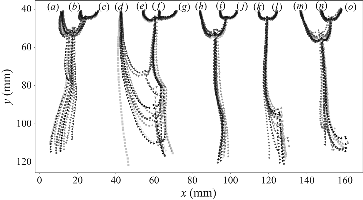
Several experiments are repeated with the same analytical initial condition (a typical evolution of the flame is displayed in figure 17a). Their evolutions are compared by focusing on the crests trajectories. The analysis starts when the forced crests become visible ( ${\approx }0.156$ s after the flow has been stopped). The crest trajectories of the 15 initial crests are then compared for 10 different runs of this experiment (figure 12). The forcing method appears to be very efficient. The initial crest locations are almost the same for the 10 different runs. Moreover, their evolution looks extremely reproducible during a time much larger than the typical time of the instability
 ${\approx }10 t_{\sigma }$. In order to quantify the similarities in trajectories, we compute the mean trajectory as
 \begin{equation} \left.\begin{array}{l@{}} x_{mean}^{i}(t)=\displaystyle{\dfrac{1}{10}\sum_{k=1}^{10}x_k^{i}(t)},\\ y_{mean}^{i}(t)=\displaystyle{\dfrac{1}{10}\sum_{k=1}^{10}y_k^{i}(t)}, \end{array}\right\} \end{equation}
where  $(x_k(t),y_k(t))$ are the coordinates of the trajectories at time
 $t$, for the run number
 $k$, and
 $i$ is the trajectory index. The error on the positions
 $\varepsilon _k(t)$ is then computed by comparing crest positions at each run to their mean
 \begin{equation} \varepsilon_k(t)=\frac{1}{15}\sum_{i=(a)}^{(o)} \sqrt{\left(x_k^{i}(t)-x_{mean}^{i}(t)\right)^{2}+\left(y_k^{i}(t)-y_{mean}^{i}(t)\right)^{2}}. \end{equation}
Crest trajectories comparison of the 15 initial crests for 10 different runs of the same experiment (each colour/symbol correspond to a different run). The crest trajectories go from top to bottom in 0.25 s ( ${\approx }10\times t_{\sigma }$). Time between each point of a trajectory
 $dt=4$ ms. The crests’ trajectories are reproducible in the first time of propagation (upper half-part of the figure). Then new crest creations (visible by sudden directional change in the trajectories) are responsible for the scattering of trajectories (d–g) and (k,l) in the bottom half-part of the figure.

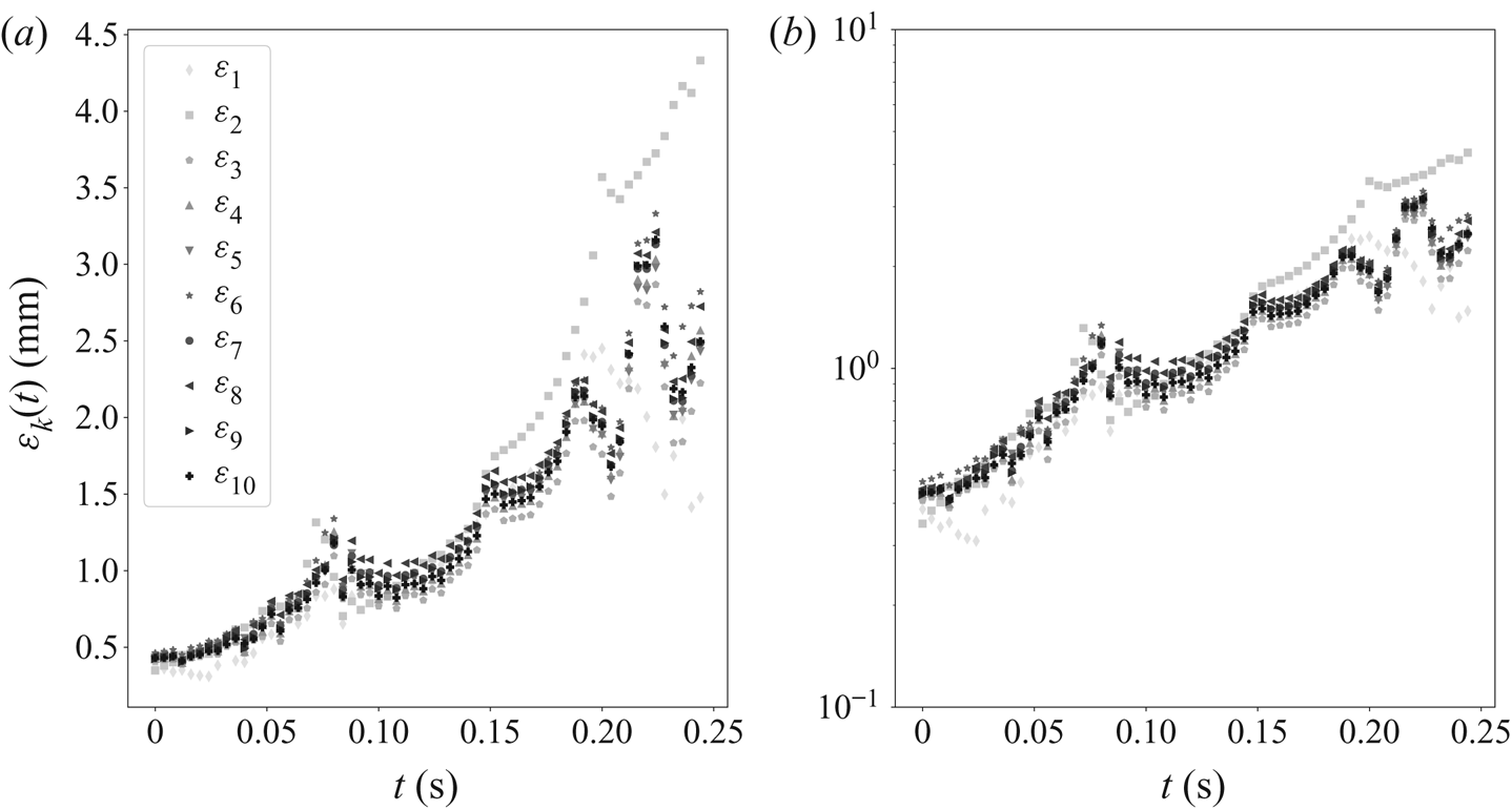
As shown in figure 13, the error on crest position follows an exponential growth. However, some peaks can be observed in the course of time, these local maxima in the error correspond to crest merging instants. Indeed, just before merging, the crests are moving fast and a small difference in the merging time induces a great difference in the distances. The analysis of the error growth curve allows us to quantify the repeatability of the flame dynamics by computing the Lyapunov exponent. For this purpose, each  $\varepsilon _k(t)$ growth curve is non-dimensionalized by the initial error and a mean non-dimensional error
 $\tilde {\varepsilon }_{mean}$ is computed as
 \begin{equation} \tilde{\varepsilon}_{mean}(t)=\frac{1}{10}\sum_{k=1}^{10}\frac{\varepsilon_k(t)}{\varepsilon_k(t=0)}. \end{equation}
The  $\varepsilon$ evolution in the course of time for each of the 10 runs. Panel (a) shows lin–lin scale; (b) semilog scale. One can observe some peaks which correspond to the cusp merging instants. Nevertheless, despite these peaks the error follows an exponential growth.

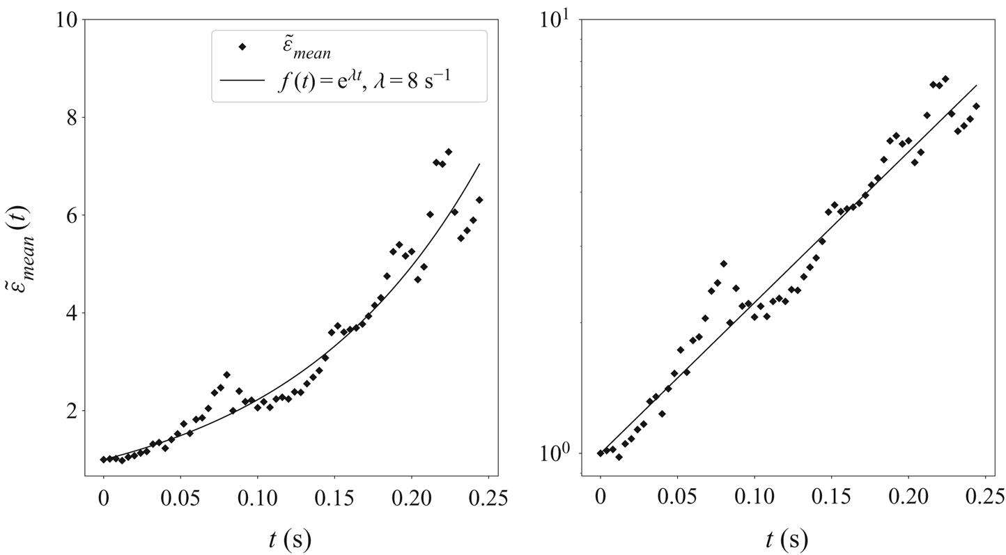
An exponential function  $\textrm {e}^{\lambda t}$ is then fitted on these data. This procedure allows us to obtain the Lyapunov exponent
 $\lambda$ (see figure 14). Here, the best fit is found to be
 $\lambda =8\ \textrm {s}^{-1}$ corresponding to a Lyapunov horizon of
 $1/\lambda =0.125$ s where
 $\lambda$ has to be compared with
 $\sigma _M\approx 60\ \textrm {s}^{-1}$. The flame dynamics can thus be described as a purely deterministic process on times much larger than the typical Darrieus–Landau time, in the fully nonlinear regime, up to the Lyapunov horizon. Far beyond this horizon, the pattern is chaotic and external noise plays an important role. In the following, by comparing the flame evolution to the one given by pole dynamics, we will show that (3.4) is relevant to describe our experiments on times shorter than
 $1/\lambda$. Later in time, the flame must be described statistically.
Evolution of the mean non-dimensionalized error in the course of time. An exponential is fitted on these data in order to determine the Lyapunov exponent of the system.

3.9. Comparison of analytical and experimental poles trajectories
Equation (3.1) is an exact solution of the flame-front problem in the limit  $\gamma \rightarrow 0$. This assumption can be considered as a crude one regarding a real flame (Kazakov & Liberman Reference Kazakov and Liberman2002b). However, as previously shown by Searby, Truffaut & Joulin (Reference Searby, Truffaut and Joulin2001), (3.1) is relevant if the parameters involved in the equation are carefully chosen. Here, following the phenomenological extension of (3.1) to arbitrary values of
 $\gamma$ proposed by Joulin & Cambray (Reference Joulin and Cambray1992), we keep the MS model in its standard form (3.1) but using the exact
 $u_A$,
 $\sigma _M$ and
 $k_c$ parameters obtained from experimental measurements.
The exact  $\sigma _M$ and
 $k_c$ values for our experiments are those previously obtained in § 3.1. A front is then extracted by image processing from an experimental capture, at early time (0.156s) (see figure 15). Then, following the procedure introduced in Almarcha et al. (Reference Almarcha, Radisson, Al Sarraf, Villermaux, Denet and Quinard2018) and providing the
 $\sigma _M$ and
 $k_c$ values determined in § 3.1, a pole solution (3.3) is fitted on the experimental front, by searching for the pole positions
 $z_n= \textrm {Re}(z_n)+\textrm {i} \textrm {Im}(z_n)$ and the amplitude
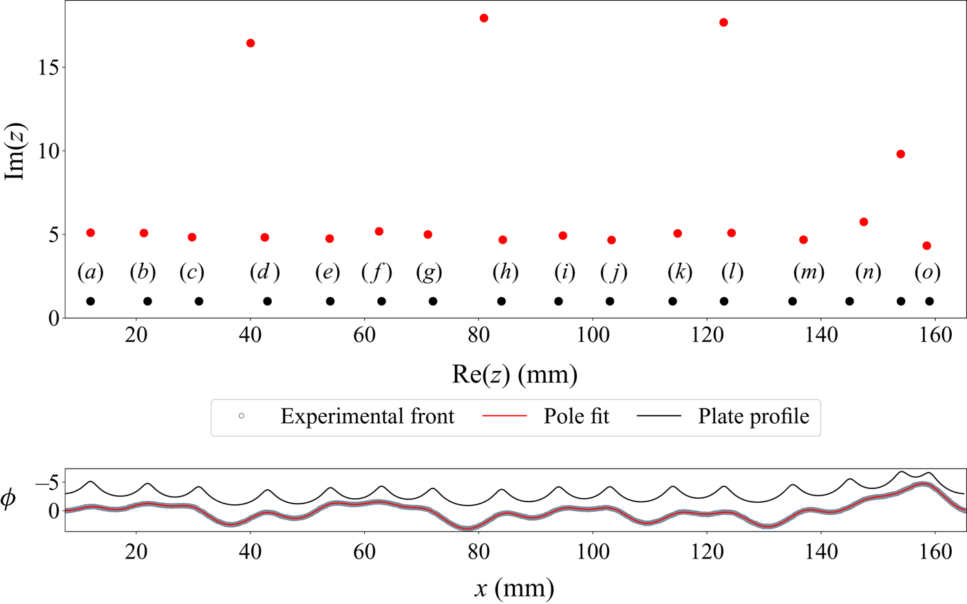
 $A$ that minimizes the error in a least square sense (see figure 15 (redline)). The first thing to note is that, although the plate profile is a
 $16$ poles solution, we have not been able to fit the experimental front with only
 $16$ poles. A minimum of
 $19$ poles has been necessary to obtain the convergence of our Levenberg–Marquardt fitting algorithm. It explains the presence of three large imaginary part poles (figure 15). As they are far from the real axis these three exceeding poles are not associated with the presence of crests but are just flattening the largest cells. Their possible influence in the dynamics will be discussed later. This solution and its corresponding poles (figure 15 (red)) are then compared with the plate profile used to force the initial condition (figure 15 (blue)). As can be seen, the
 $\textrm {Re}(z_n)$ positions of the 15 nearest poles to the real axis (figure 15 (red dots)) are almost identical to the expected poles positions (figure 15 (blue dots)). However, one can note that their imaginary parts,
 $\textrm {Im}(z_n)$, are substantially larger (
 ${\approx }5\times$) than those associated with the plate profile. As a consequence, the profile on the plate is more cusped than the flame profile. This difference can be adjusted with the distance between the plate and the initial anchored inverted-V flame. The closer the plate, the more pronounced are the cusps in the initial flame profile. To summarize, the plate method allows us to introduce some poles at given
 $\textrm {Re}(z)$ positions but with low control on their
 $\textrm {Im}(z)$ location. Moreover, in § 3.7, we argued that the two last crests on the right-hand side of the forced solution could have merged in one (crest
 $(o)$) due to the merging of the two corresponding poles before they have been attracted toward the real axis. This statement is actually corroborated by the fitted solution, where two poles form a pile at the
 $(o)$ crest position.
Comparison of the forcing plate profile (black line and black dots) with the experimental front (grey circles) and its best pole decomposition (red line and red dots) obtained by a Levenberg–Marquardt fitting algorithm. The amplitude has been multiplied by a factor of  $5$ for the experimental front and the fitted solution. The nearest poles to the real axis are responsible for crests at same abscissa on the front, whereas the further are flattening the larger cells.

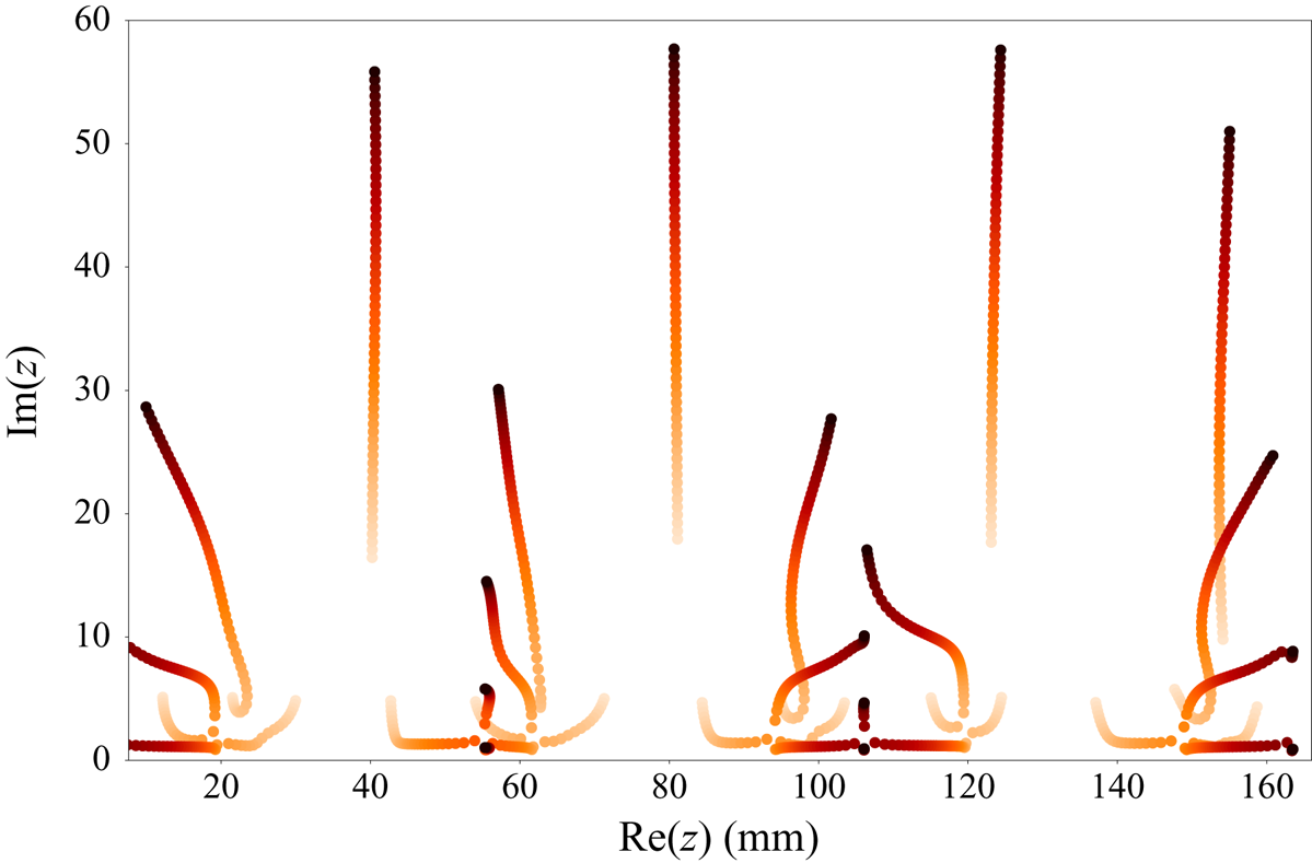
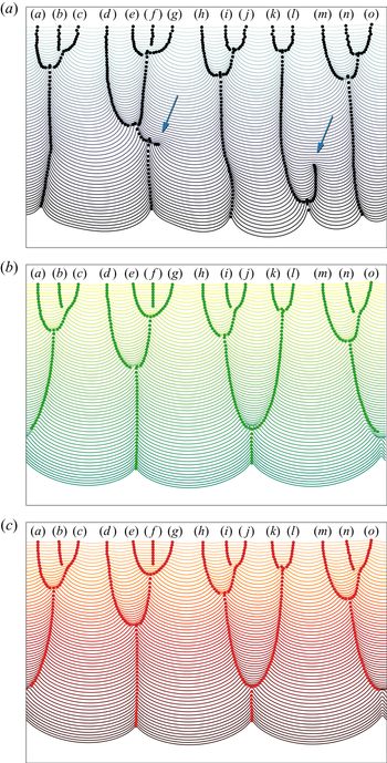
Since an accurate pole decomposition of the experimental front has been obtained, the dynamics described by (3.4) can now be compared with the experimental evolution. For this purpose, starting from the fitted solution (figure 15 (red dots)), the system of ordinary differential equations (3.4), is numerically integrated thanks to a fourth-order Runge–Kutta algorithm. This integration gives the pole trajectories in the complex plane (figure 16). At each instant of the evolution, the flame front is then obtained from the current position of the poles using (3.3). The resulting flame-front evolution is shown in figure 17(c). The latter is compared with the evolution given by MS pseudo differential equation (PDE) integration (3.1) (figure 17b), starting from the initial experimental front. The evolution given by the pole dynamics and the one given by MS PDE are nearly identical. This observation attests to the quality of the fit realized in figure 15. Moreover, these two evolutions obtained from the MS model agree well with the experimental one during, approximately, the half-part of the plot ( ${\approx }0.125$ s). This typical time corresponds to the Lyapunov horizon determined in § 3.8. Beyond this characteristic time the system loses memory of the initial condition and become unpredictable.

Comparison between experimental evolution of a propane–air flame  $\varphi =0.8$ and the corresponding evolution given by the MS PDE and by pole dynamics. (a) Typical experimental evolution obtained by forcing an initial condition using the pole profiled plate method. (b) Corresponding evolution given by MS PDE, starting from the initial experimental front. (c) Corresponding evolution given by pole dynamics, starting from the pole solution corresponding to the initial experimental front. Flame goes from top to bottom in 0.25 s. Time between each front
 $dt=4$ ms.

During the first half-part of the evolution, the 15 poles associated with crests are first attracted toward the real axis (figure 16), leading to a more cusped front (see figure 17). Then, due to the horizontal interaction, they attract each other, pilling up at same abscissas. This process is the mechanism responsible for the merging of crests observed in the experiments.
During the second half-part of the propagation, the crests trajectories described by pole dynamics are diverging from the experimental ones. This is actually due to the already mentioned issue of new cusp creation. Looking at figure 17, one can observe two crest creations (pointed out by arrows). These new cusps are responsible for the disparity in crest trajectories, observed in the previous section (see figure 12). As quoted before, these new crests may come from poles originally far from the real axis that have been attracted toward the real axis (see figure 7), or by an external forcing responsible for the injection of new poles in the system. However, if the latter is true, one can note that these new crests are appearing always in the same zone for the 10 experimental runs considered in the present paper (see figure 12). Then, if an external noise is responsible for the appearance of these new crests, it means that the flame possesses regions that are more sensitive to noise than others, otherwise new crests come from poles which were initially present. In that case, one can ask about the three exceeding poles in the fitted initial solution. We can postulate three different interpretations for their presence: (i) the pole decomposition (3.3) is a too simplistic description regarding real flames and therefore we have not been able to fit the flame with just one pole at each crest; (ii) the exceeding poles have been embedded by an external source of noise during the first instant of propagation; (iii) the plate forcing method is not accurate enough and inserted some undesirable poles. These exceeding singularities could be responsible for the formation of new crests observed in the experiments. However, to make new crests, these poles should be attracted toward the real axis and it is obviously not what is predicted by (3.4) (see figure 16). The additional poles are rapidly spurned to  ${\pm }i\infty$, and never lead to the generation of new crests (see evolution on figure 17). Indeed for the present case,
 $\Lambda /\lambda _c=1/\nu =21.4$, corresponding to an optimal number of poles of
 $N_{opt}=11$ (see Thual et al. Reference Thual, Frisch and Hénon1985). Therefore, initially, there are eight poles in excess that have to be pushed away from the real axis. This explains why these poles are not attracted toward the real axis. Nevertheless, some key features such as gravity or heat loss effects are not taken into account in the MS model and may be responsible for slight modifications in the pole dynamics, eventually leading to the attraction of exceeding poles toward the real axis. Yet, the latter remark is purely speculative as until now no pole description that takes gravity effects into account has been obtained.
As presumed, the generation of new crest is a key component in the flame dynamics and is responsible for the non-repeatability of the crest trajectories, and thus to the failure of a pole dynamics forecast after some time of evolution.
4. Late-time evolution
4.1. Expected cell size distribution
As shown in the previous section, the deterministic stage of large-scale flames ends after the Lyapunov horizon  $1/\lambda$, when new crests creations arise. The dynamics is then sensitive to external forcing (e.g. thermal noise, residual turbulence or vibrations) or to self-generated large-scale perturbations, and must be studied as a stochastic process. As explained in Cambray et al. (Reference Cambray, Joulain and Joulin1994), when a cell gets sufficiently large, a new crest appears and splits the cell in two. As a result, instead of continuously growing up to the size of the domain of propagation, the mean cell size saturates to a stationary value that decreases when the forcing noise intensity increases. Moreover, when changing the properties of the reacting gas, the mean cell size is also expected to vary. We focus here on the distribution of the cells sizes around the mean. As the problem is composed of two competing phenomena, the new crests generation that dominates on large cells, and the crest coalescence that dominates at small scale, we can expect a stationary distribution as demonstrated in Escobedo, Mischler & Ricard (Reference Escobedo, Mischler and Ricard2005). Assuming that the cells split at random, the tail of the distribution (for large cells where fragmentation dominates) is expected to have an exponential decay
 \begin{equation} p\left(d\gg\left\langle d\right\rangle\right)\propto \textrm{e}^{-d}.\end{equation}
At small scales, the coalescence of cusps dominates and is described by (3.9) so that the probability of occurrence of each scale is proportional to its lifetime during the kinematic coalescence process. This lifetime is inversely proportional to the rate of variation of the size in time during coalescence, namely  ${\mathrm {d} d}/{\mathrm {d}t}=-{32\sigma _M}/{k_c^{2} d}$ according to (3.9), so that
 \begin{equation} p\left(d\ll\left\langle d\right\rangle\right)\propto \frac{k_c^{2} } {32\sigma_M}d. \end{equation}
The whole distribution is expected to respect the two conditions, (4.1) and (4.2), and therefore to follow a gamma distribution (Villermaux & Duplat Reference Villermaux and Duplat2003) as introduced in Almarcha et al. (Reference Almarcha, Radisson, Al Sarraf, Villermaux, Denet and Quinard2018),
 \begin{equation} p\left(x=\frac{d}{\left\langle d\right\rangle}\right)=\frac{4}{\Gamma(2)} x \,\textrm{e}^{-2 x}. \end{equation}
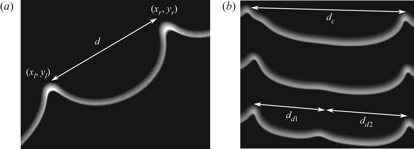
In order to compare this theoretical prediction for the cell size distribution, we carried out both numerical and laboratory experiments. Both for the fronts extracted from numerical simulations and those extracted from experimental images, crest positions are localized by way of a continuous wavelet transform method (Du, Kibbe & Lin Reference Du, Kibbe and Lin2006). The cell size distribution is then computed by measuring the distance between each crest,  $d=\sqrt {(x_r-x_l)^{2}+(y_r-y_l)^{2}}$ (see figure 18).
(a) Typical measure of a cell on a propane–air flame  $\varphi =0.8$. Field of view: 30 mm. (b) Cell of size
 $d_c$ giving birth to two daughter cells of size
 $d_{d1}$ and
 $d_{d2}$ by splitting.

4.1.1. Numerical experiments
The numerical experiments are performed in the MS framework to allow large-scale flame simulations for a limited cost. The non-dimensional Sivashinsky equation (3.11) is integrated by way of Fourier pseudospectral method (Giada, Giacometti & Rossi Reference Giada, Giacometti and Rossi2002), starting from a flat front with small amplitude white noise and periodic boundary conditions. The integration in time is performed by way of the finite difference method with a semi-implicit scheme (forward/backward Euler). The simulations are carried out over a large time  $t\gg t_\sigma$ in order to have a large statistical sampling to compute the cell size distribution. As stated before, the emergence of new crests are related to a sensitivity to external perturbative noise which can be round-off errors, for instance. In order to test the influence of the noise intensity on the cell size distribution, we integrated the following forced MS equation (pseudospectral method domain of width
 $\Lambda =2{\rm \pi}$ with 2048 Fourier modes and time step
 ${\rm \Delta} t=10^{-5}$):
 \begin{equation} \Phi_{\tau}+\tfrac{1}{2}\Phi_X^{2}=\nu \Phi_{XX}+ I\left(\Phi, X\right)+ \eta(x, t), \end{equation}
with  $\eta (x,t)$ a Gaussian white noise probability density function
 \begin{equation} f(\eta)=\frac{1}{s\sqrt{2{\rm \pi}}}\exp\left(-\frac{\eta^{2}}{2s^{2}}\right).\end{equation}
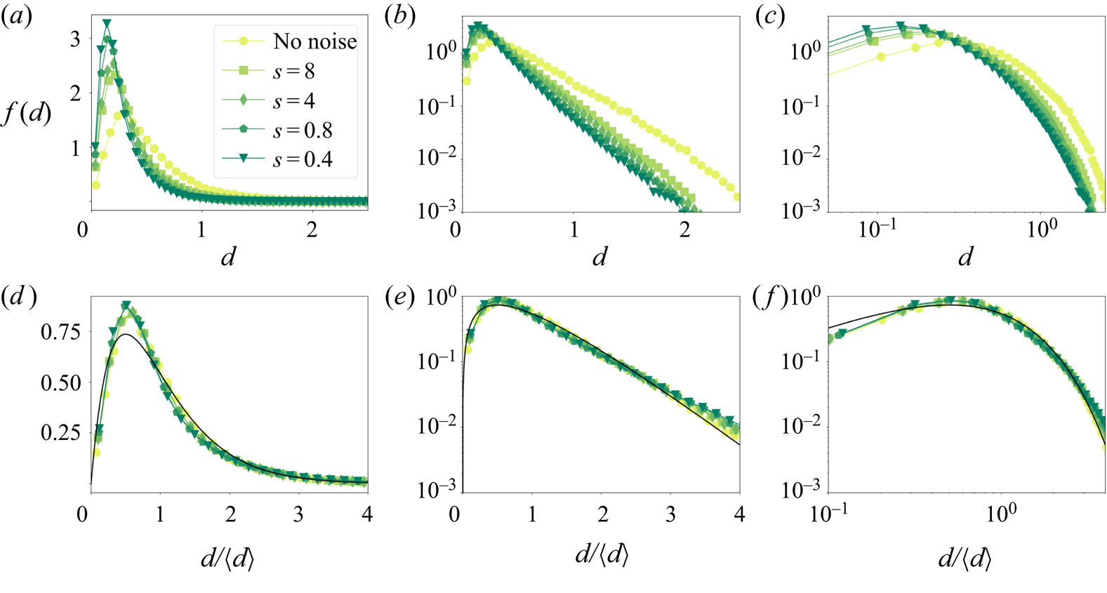
The cell size distribution is then computed following the procedure described earlier, from simulations with different noise intensities. The corresponding results are plotted in figure 19. One can see that even if the noise intensity has a strong influence on the mean cell size, the non-dimensional distribution is not affected and is perfectly matching the expected law (4.3)
Cell size distributions computed from forced MS simulations (see (4.4)) on a domain of width  $\Lambda =2{\rm \pi}$ with periodic boundary conditions and
 $2048$ Fourier modes and time step
 ${\rm \Delta} t=10^{-5}$. For all the simulations only the noise intensity is varied, the unstable mode number is fixed to
 $1/\nu =200$. (a) Dimensional cell size distribution lin–lin scale. (b) Dimensional cell size distribution semilog scale. (c) Dimensional cell size distribution log–log scale. (d) Non-dimensional cell size distribution lin–lin scale. (e) Non-dimensional cell size distribution semilog scale. (f) Non-dimensional cell size distribution log–log scale.

4.1.2. Experiments in the Hele-Shaw burner
The experiments are performed in the apparatus described in § 2 using the experimental procedure described in § 2.1. The high-speed Photron camera (field of view  $50\ \textrm {cm} \times 50\ \textrm {cm}$) is placed between
 $y=75$ and
 $y=125$ cm under the top of the burner, in order to be far from the first instants of propagation and reach fully developed dynamics, and to be far from the closed end of the burner (to avoid confinement effects on the unburned gas side). The experiments are performed with propane–air mixtures for a large range of equivalence ratios (
 $0.8<\varphi <1.3$). For each mixture the experiments are repeated approximately 30 times in order to have a large statistical sample (
 ${\approx }10^{4}$ occurrences for each mixture). Moreover, the acquisition frame rate
 $1/t_{frame}$ of the high-speed camera is adjusted in order to be large enough with respect to the observed dynamics
 $t_{frame} \approx 0.5 t_{\sigma }$. The flame fronts are extracted from these images using the procedure described in § 2.4.
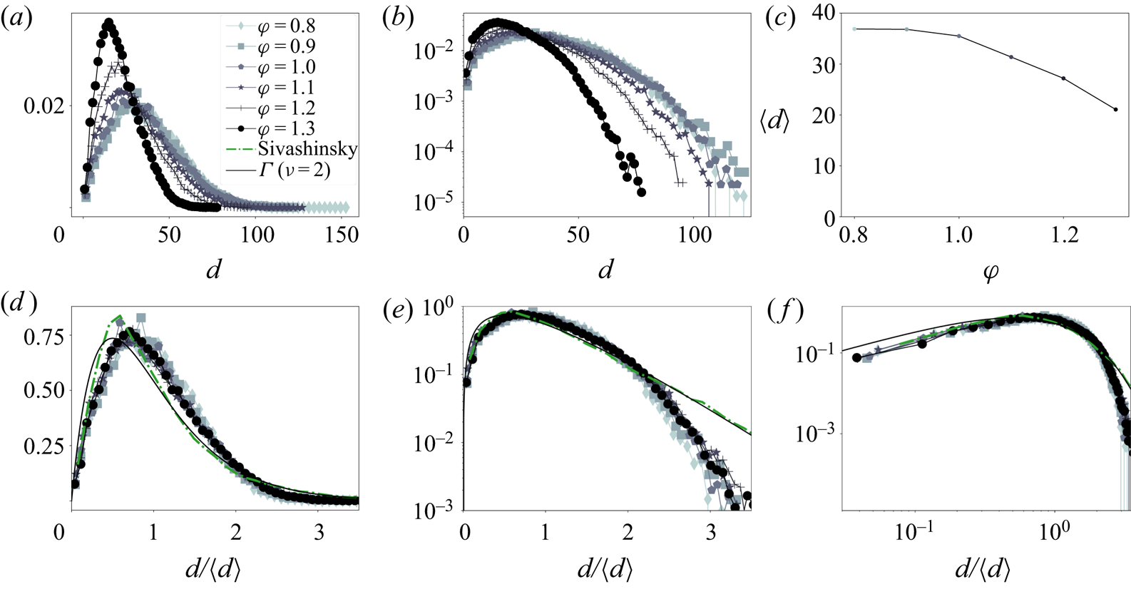
The results obtained numerically and experimentally are presented in figure 20. First, by comparing with growth rate measurements in Al Sarraf et al. (Reference Al Sarraf, Almarcha, Quinard, Radisson and Denet2018a) and Al Sarraf et al. (Reference Al Sarraf, Almarcha, Quinard, Radisson, Denet and Garcia-Ybarra2018b), one can note that, as first observed by Markstein (Reference Markstein1949), the mean cell size  $\left \langle d \right \rangle$ is much larger than the most unstable wavelength
 $\lambda _{max}$ (
 $\left \langle d \right \rangle \approx 5\lambda _{max}$) predicted by the linear theory. Furthermore, due to thermodiffusive properties of the C3H8–air mixture,
 $\left \langle d\right \rangle$ is noticeably decreasing when the equivalence ratio is increased (figure 20a–c). However, despite the variations of the mean size with the equivalence ratio, all the cell size distributions collapse on a same curve when non-dimensionalized by the mean cell size
 $\left \langle d \right \rangle$ (see figure 20d–f). This self-similar property is a common feature of a Smoluchowski aggregation process (Swift & Friedlander Reference Swift and Friedlander1964; Hidy Reference Hidy1965; Friedlander & Wang Reference Friedlander and Wang1966; Fournier & Laurençot Reference Fournier and Laurençot2005). However, although the experimental distributions all collapse on the same curve, one can note a significant lack of large cells regarding the cell size distribution obtained numerically and the theoretical distribution given by (4.3). As this discrepancy concerns lengths much larger than the mean, we can expect that the splitting mechanism is different in the numerics and in the experiments. We can expect that the experimental large-scale cells are relatively more prone to split than the numerical ones. In order to confirm this tendency, we identify the new crest appearance and measure the size
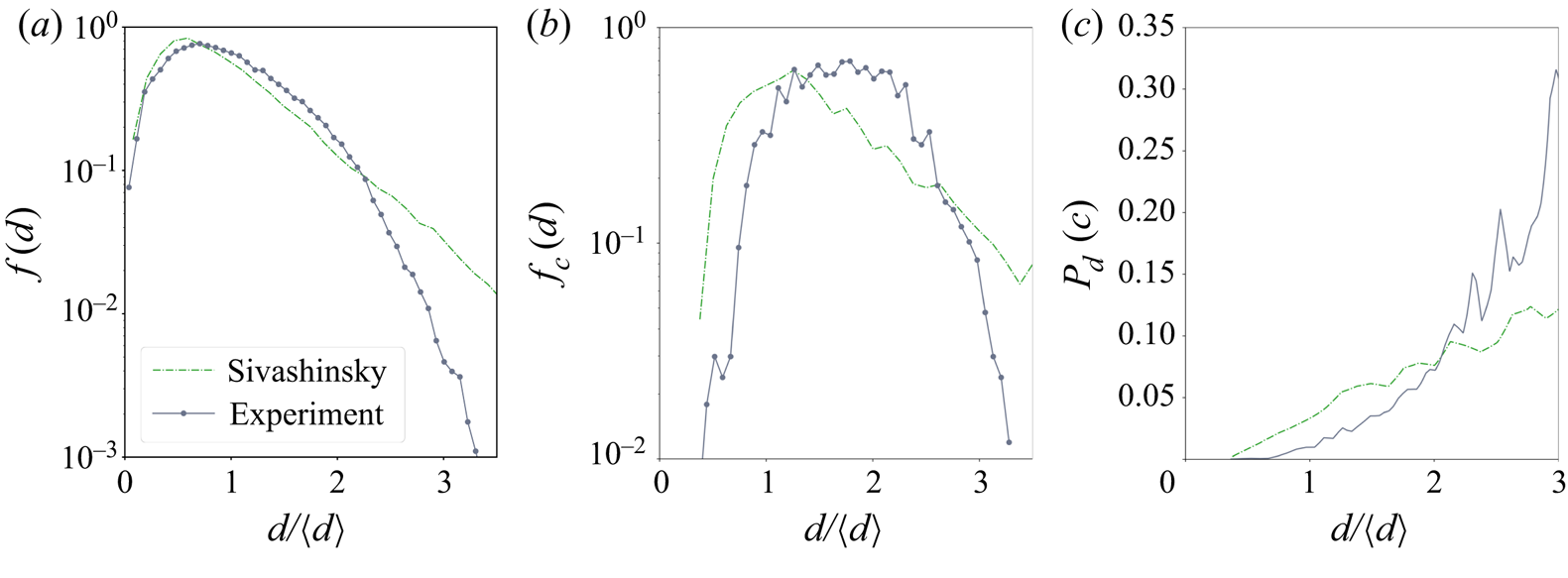
 $d_c$ just before cells split (see figure 18), either from experimental or numerical fronts. The distribution of the cells that split is reported in figure 21(b). Of course, such a distribution is linked to the probability of presence of each cell in figure 21(a). In particular, few cells are splitting for sizes
 ${d}/{\left \langle d\right \rangle }>3$ mainly because very few of these big cells are present along the flame front. In order to determine the natural tendency for each cell to break depending on their size, we divide the distribution in figure 21(b) by the distribution in figure 21(a) to obtain figure 21(c). The result is related to the lifetime expectation or conversely, to the probability per unit time for a specific cell to break when it is of size
 $d$, which according to Bayes’ theorem (Bayes, Price & Canton Reference Bayes, Price and Canton1763; Laplace Reference Laplace1774) is given by
 \begin{equation} P_d(c)=\frac{P_c(d)P(c)}{P(d)}, \end{equation}
with  $P_c(x=d \in [a,b])=\int _{a}^{b}f_c(x)\, \textrm {d} x$ the probability that a cell splits given it is of size
 $d$,
 $P(c)$ the probability of splitting and
 $P(x=d \in [a,b])=\int _{a}^{b}f(x)\, \textrm {d} x$ the probability for a cell to be
 $d$ in size, giving
 \begin{equation} \Leftrightarrow P_d(c)=\frac{f_c(d)P(c)}{f(d)}. \end{equation}
Experimental cell size distributions for propane–air flame at different equivalence ratio compared with theoretical and numerical ones. (a) Dimensional cell size distribution lin–lin scale. (b) Dimensional cell size distribution semilog scale. (c) Mean cell size evolution with equivalence ratio. (d) Non-dimensional cell size distribution lin–lin scale. (e) Non-dimensional cell size distribution semilog scale. (f) Non-dimensional cell size distribution log–log scale.

Cell splitting statistics. (a) Non-dimensional cell size probability density function for experimental and numerical (MS) fronts. (b) Probability density function of cell size which splits. (c) Probability to split per time unit for a given cell of size  $d$, as a function of
 $d$.

This quantity is displayed in the last plot of figure 21. The difference, between experimental and numerical results, in the way external perturbations affect cell splitting is now made very clear. Indeed, for Sivashinsky simulations, the probability of splitting for a given cell of size  $d$ exhibits a linear growth with
 $d$, which is compatible with a probability of breaking, per unit length, which is constant. This particular property is the signature of a random splitting mechanism along the flame front. Conversely, for experimental flames, the probability grows faster than linearly with cell size, showing that a cell is more sensitive to noise when it becomes larger. This characteristic reveals the presence of a mechanism, acting specifically on large cells, that breaks the random splitting hypothesis. A probable candidate is the gravity field that may flatten the largest cells by a buoyancy effect and make them more sensitive to noise. Another candidate is the heat loss on the glass plates behind the flame that may decrease the Darrieus–Landau effect for large cells and especially cells much larger than the cooling length. The analysis of these effects shall be addressed in a forthcoming study.
5. Conclusion
For nearly one hundred and fifty years premixed flames have been known to exhibit a cellular pattern. Despite many attempts to characterize theoretically and experimentally their evolution and scalings, there was no robust and complete mechanism to explain the properties and the evolution of such a pattern. As the combustion process involves a complex reactive fluid dynamics with strong density gradients, the major part of the studies has tried to tackle the question with the help of simplified models, by considering the flame as a gasdynamic discontinuity, between two flows of different densities (Frankel & Sivashinsky Reference Frankel and Sivashinsky1982; Matalon & Matkowsky Reference Matalon and Matkowsky1982; Pelce & Clavin Reference Pelce and Clavin1982). In this framework much effort has been made to obtain an equation for this interface in a closed form (i.e. in a form involving only quantities defined on the flame front) (Sivashinsky Reference Sivashinsky1977; Sivashinsky & Clavin Reference Sivashinsky and Clavin1987; Joulin & Cambray Reference Joulin and Cambray1992; Bychkov Reference Bychkov1998; Bychkov & Kleev Reference Bychkov and Kleev1999; Bychkov, Kovalev & LibermanReference Bychkov, Kovalev and Liberman1999; Kazakov & Liberman Reference Kazakov and Liberman2002a,b Reference Kazakov and Liberman; Kazakov Reference Kazakov2005a,b Reference Kazakov; Joulin, El-Rabii & Kazakov Reference Joulin, El-Rabii and Kazakov2008; El-Rabii, Joulin & Kazakov Reference El-Rabii, Joulin and Kazakov2010; Assier & Wu Reference Assier and Wu2014). However, to obtain such an equation is an extremely intricate mathematical problem because it requires solving the whole flow both ahead and behind the flame front. Therefore, to obtain such an equation generally requires some strong assumptions. One of them consists in developing all the quantities involved in the problem in the small expansion limit. Despite such a crude assumption, the obtained equation was already known for years to reproduce, qualitatively well, the essential features of flame dynamics observed in experiments. Moreover, the obtained nonlinear equation admits pole solutions, which make the dynamics analytically tractable. However, until now there was no experimental evidence of its validity on fully developed nonlinear stages. In most experimental facilities used previously the flame front consisted of a three-dimensional reaction sheet, and the analysis of the front properties is an extremely difficult task.
In this study we use a simplified apparatus that constrains the dynamics to two dimensions only, and despite the heat and momentum losses induced by the confined geometry, the flame dynamics remains of the same nature as in three-dimensional geometries. Thus, the flame-front analysis is greatly simplified, and its description is more accurate. For instance, the experimental tracking of two crests merging has been successfully compared with an expected analytical model of  $d^{2}$ law.
In addition, we used an improved version of a technique recently introduced by Al Sarraf et al. (Reference Al Sarraf, Almarcha, Quinard, Radisson and Denet2018a) where a forcing plate at the top of the burner creates a wrinkling of the flame front. Using a plate machined by laser-cutting, we are now able to print perturbations on the flame front, and to impose precisely the position of the crests that will develop. Thanks to this method, the experimental repeatability has been studied, by performing the experiments several times from the same forced initial condition. The largest Lyapunov exponent of the system has been computed by analysing these experiments. It allows us to identify the characteristic time (the Lyapunov horizon), beyond which the flame dynamics is no longer predictable. When the initially imposed perturbation is an analytic solution of the MS model (i.e. a pole solution), we demonstrated that it is possible to impose the whole analytic nonlinear trajectory to the flame front for times as late as a decade further than the linear growth time. It is a great demonstration of the astonishing accuracy of the pole description.
Later in time the external perturbations play an important role. Moreover, the front is prone to develop large slopes, therefore the MS model is valid locally only. Nevertheless, we have highlighted that for the statistically stationary late-time dynamics, the elementary pole attraction is still ruling the pattern through an aggregation process combined with a fragmentation process. This fragmentation is inducing the large cells statistic decay. In the case of the MS equation forced with additive white noise at random, a gamma distribution was obtained whatever the noise intensity. In the experiments, a faster decrease of the distribution was obtained, expressing that large cells have an enhanced tendency to break, certainly due to gravity or heat loss effects.
Finally, a perspective opened by this study is to extend the present work to three-dimensional flames. Here again, as the analysis of three-dimensional experimental flames is intricate, numerics seems to be the best way to achieve it. In the MS framework, it has been shown that because of the nature of the nonlinear term involved in the MS PDE, the dynamics in  $x$ and
 $y$ directions are completely independent (Denet Reference Denet2007), therefore the analysis carried out in this paper is still valid. However, the
 $x$ and
 $y$ dynamics should be coupled for finite
 $\gamma$ values. To investigate this question, the recent extension of the fully nonlinear model introduced in Rastigejev & Matalon (Reference Rastigejev and Matalon2006b) to three-dimensional geometry (Patyal & Matalon Reference Patyal and Matalon2018) is really promising for large-scale flame dynamics analysis.
Acknowledgements
We would like to thank P. Le Gal, E. Villermaux and G. Joulin for many stimulating and fruitful discussions and É. Bertrand for valued technical support. We are also grateful to the ‘Agence Nationale de la Recherche’ for funding of the ANR ‘PDF’ ANR-14-CE05-0006, the Excellence Initiative of Aix-Marseille University–A*MIDEX, and Labex MEC, for funding.
Declaration of interests
The authors report no conflict of interest.