1. INTRODUCTION
The permutation flowshop scheduling problem (PFSP) is a well-known scheduling problem in many industries, such as steel making, food processing, pharmaceutical, automobile, wooden furniture, and Sanitaryware. Even though flowshop research is widely studied from a theoretical perspective, there are still weaknesses when solving many practical problems that arise on the production floor. Often these problems are more difficult to solve because of additional characteristics and constraints, such as setup times, product specifications, batch size, and capacity constraints. These factors have motivated us to study this case of a real-world flowshop scheduling problem.
Most of the research on production and operations management have classified production systems into two categories: make-to-order (MTO) and make-to-stock (MTS) production systems (Rahman et al., Reference Rahman, Sarker and Essam2015). An MTO production system is more customer specific and usually produces expensive products. In this case, production planning involves order acceptance or rejection decisions, while considering capacity planning, order arrival time, and delivery time or due dates. In contrast, MTS production systems usually focus on less expensive products with low variety. The production planning of a typical MTS system considers anticipating demands, planning to meet such demands, batch size of each product, and length of production cycle.
The case study presented in this paper refers to an MTO Sanitaryware production system. This system is a kind of permutation flowshop. Focusing on this particular production plant, the production scheduling problem is complex and time sensitive, because the decision making depends on random interarrival time and due dates of customer orders without prior information about the composition of orders (product category and their quantity), setup times, due date, and production capacity constraints. Regarding all customer order related performance measures, product diversity, and time sensitivity of operation, the current production plant is often run with a suboptimal solution. Due to this frame of condition, in this paper we have proposed a memetic algorithm based real-time strategy to schedule tasks of the investigated Sanitaryware production line. In order to test the performance, some test instances from the practical production scenario have been generated. To evaluate the performance of the proposed approach, an upper and lower bound have been proposed. The results of thorough analysis allow us to identify the superiority of the proposed approach with respect to existing practices.
2. MTO-BASED SANITARYWARE PRODUCTION SYSTEM
As described earlier, the case refers to a Sanitaryware production plant, which is located in Bangladesh. The production system is capable of producing 10 different types of products, which are listed in Table 1. Based on the specification of the customers, each order consists of a mix of different products with different product volumes; for example, an order may consist of a total of 10 products, where 3 products are from wash basins, 5 products are from galleries, and 2 are kitchen sinks. Production of Sanitaryware follows a series of operations. At the beginning, harder raw materials (e.g., quartz stone, lime stone, feldspar) are crushed through jaw crushers, and bigger and smaller particles are separated through different vibrating separators. Then, these particles are passed through a ball mill where harder particles are mixed with soft materials (e.g., bejoy clay, china clay, ball clay) in a proper ratio. From the ball mill, the mixtures are transferred to the blunger, where sufficient amounts of water are added to increase fluidity. Then the mixture is passed though a magnetic separator to remove any magnetic particles from the solutions. In the next step, different products are given into different shapes through different dies in a casting process. The next step for Sanitaryware is drying, where the casted materials are dried at an elevated temperature, and then the dried products are retouched and cleaned. The cleaned semifinished products are glazed with certain chemical solutions that improve the smoothness of the surface and also reduce porosity. This is followed by firing, where the products are heated through some Kline furnaces. Next, in accordance to specifications and quality, products are sorted, grinded, and cleaned. Finally, finished products are packaged, and the production process completes.
Product types

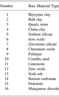
An MTO Sanitaryware production system consists of four phases: planning stage, input, production process, and products. In the planning stage, order acceptance/rejection and scheduling decisions of an incoming order are made. If the order is accepted, production process is initiated with input, and this includes raw materials and utilities (electricity, water, gas, etc.). The raw materials are listed in Table A.1 in Appendix A. Inputs have been processed through the different stages of a production process, and after adding values in these stages, all products of each order will have been produced.
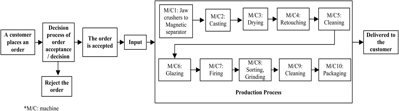
Figure 1 presents a production flow diagram of an MTO Sanitaryware manufacturing system. Like other MTO systems, customers place orders with specific delivery times or due dates. Once a customer places an order, the production manager has to make two decisions: an order acceptance or rejection and scheduling the accepted order. The first decision depends on the availability of production capacity to produce the products within its due date at the point in time when it arrives at the production plant. The available production capacity depends on the accepted orders waiting to process and currently under process. Here, an accepted order starts to process in the first machine (from jaw crusher to magnetic separator) as soon as it is free. The second decision depends on sequencing the accepted products in all machines. Note that from the jaw crusher to the packaging stage, the production floor consists of 10 machines in series. Each product can be considered as a job. Each product needs a specific time to set up in each machine, like mold installment and adjustment in the casting machine, preparation of specific chemical solution, and preheating the firing Kline. However, after processing a product from the same family or category in a particular machine, the setup time of the next product is zero on the same machine if the product is from the same family. Besides, if a product from a certain product family does not need to be processed in a certain machine, the setup time and processing time of that product on that particular machine is zero. For example, each pedestal does not require processing in machine-8 (grinding and sorting), so setup and processing time of pedestals on this machine is zero.
Production flow of a typical make-to-order Sanitaryware production system.

If each product family allows one setup (or single batch per each type of product per order), setup time or cost is minimum. However, the completion time or makespan of an order may be improved if all products are scheduled together while allowing multiple setup of the same product category. In contrast, the setup time on each machine adds additional time, which may increase the completion time or makespan. Setup time is a key factor in scheduling an order, and the number of setups for each product family should be adjusted on a real-time basis. Finally, after processing in all stages, an order is instantly delivered to its customers. The production plant runs for a certain amount of time (like production per day or week), which is called a production shift, and within a production shift, the company receives a certain number of orders.
After processing and delivering an accepted order, a company can earn certain amount of profit. Otherwise, an opportunity loss cost reduces the overall profit of the company.
3. RELATED LITERATURE
In this section, we briefly discuss the research relevant to the current study. Since Johnson (Reference Johnson1954) first introduced the flowshop scheduling problem as an interesting industrial problem, it has attracted many schedulers and practitioners. The classical optimization techniques were popular approaches for solving small-scaled ideal PFSPs with the current computational power. For solving large-scale problems, academic research focus on heuristics (Nawaz et al., Reference Nawaz, Enscore and Ham1983) and meta-heuristics algorithms (Ogbu & Smith, Reference Ogbu and Smith1990; Nowicki & Smutnicki, Reference Nowicki and Smutnicki1996; Grabowski & Wodecki, Reference Grabowski and Wodecki2004; Rajendran & Ziegler, Reference Rajendran and Ziegler2004; Onwubolu & Davendra, Reference Onwubolu and Davendra2006; Ruiz et al., Reference Ruiz, Maroto and Alcaraz2006; Tasgetiren et al., Reference Tasgetiren, Liang, Sevkli and Gencyilmaz2007; Zobolas et al., Reference Zobolas, Tarantilis and Ioannou2009; Rahman et al., Reference Rahman, Sarker and Essam2013). The ideal PFSP is basically a single-order PFSP where the task is to schedule a set a job (an order) in a set of machines. However, in practical MTO system, production managers often receive a stream of orders or a certain pool of orders from which certain orders may be accepted and scheduled with respect to the limited machine capacity (Slotnick, Reference Slotnick2011). If the scheduler accept all orders without checking the feasibility for on-time completion, it will isolate the overall mission of the company that would lead to reduced revenue (Guerrero & Kern, Reference Guerrero and Kern1988). Over the past few decades, the order acceptance and scheduling problem has been studied in a static single machine environment where the arrival times due dates of each order are known well in advance (Rom & Slotnick, Reference Rom and Slotnick2009). The next level of complexity is the order acceptance and scheduling problem in multiple machine environments. Even though these problems are more complex and practical, only a handful of studies in the literature have addressed these problems (Xiao et al., Reference Xiao, Zhang, Zhao and Kaku2012; Wang et al., Reference Wang, Xie and Cheng2013), and there are limitations in the studies, such as: the order acceptance and scheduling decisions have been made separately. However, these decisions process relates to each other, and the studies only consider static order acceptance and scheduling problem in static multiple order problems in MTO environments. However, in actual manufacturing environment, orders may randomly arrive into the production system, with no prior knowledge about the order compositions, due dates, and arrival time (Pinedo, Reference Pinedo2012).
Over the past decades, a huge amount of work has been published dealing with the diverse aspects of the scheduling problem. However, there is still a decent “gap” between theoretical approaches and actual practice in industries. To reduce this gap, Graves (Reference Graves1981) proposed some possible approaches. At the time of their studies, Ford and Bradbard (Reference Ford and Bradbard1987) showed that the applications of some theoretical approaches were impossible to implement in practice. Some researchers have criticized the limited practical applicability of flowshop research in particular (Dudek et al., Reference Dudek, Panwalkar and Smith1992). A statistical review presents an interesting review of flowshop scheduling research, and found that only 3% of studies considered real production systems (Reisman et al., Reference Reisman, Kumar and Motwani1997). Parthasarathy and Rajendran (Reference Parthasarathy and Rajendran1997) studied a real-life flowshop problem with the objective of minimizing maximum weighted tardiness. Bertel and Billaut (Reference Bertel and Billaut2004) developed a mixed integer programming model for a practical three-stage hybrid scheduling problem and proposed a heuristic to solve it. Ruiz et al. (Reference Ruiz, Serifoglu and Urlings2008) developed a flexible flowshop model with realistic constraints. However, even though a few attempts have been taken to solve real-life scheduling problems, to our best knowledge, no attempt has been taken to solve a practical make-to-order PFSPs. Note that multiple-order PFSPs are common in real-life production environments, such as steel, ceramic, Sanitaryware, and bakery production. However, in reality, each machine may require a specific time to set up before it starts to process a job or manufacture a different product. A few researchers have addressed setup time for single-order PFSPs (Allahverdi, Reference Allahverdi2000; Glass et al., Reference Glass, Shafransky and Strusevich2000; Al-Anzi & Allahverdi, Reference Al-Anzi and Allahverdi2005; Brucker et al., Reference Brucker, Knust and Wang2005; Allahverdi & Al-Anzi, Reference Allahverdi and Al-Anzi2006; Ng et al., Reference Ng, Allahverdi, Al-Anzi and Cheng2007). These studies are limited to single-order PFSP with setup times with small-scaled problems (like two-machine PFSPs), and all the problems considered a static permutation flowshop. Another brief review on this topic can be found in Allahverdi et al. (Reference Allahverdi, Ng, Cheng and Kovalyov2008).
To our best knowledge, the only related work to set up in a dynamic flowshop is Su and Chou (Reference Su and Chou2000)'s work. They studied a two-machine PFSP with the objective of total flow time minimization with weighted sum of makespan in a dynamic environment where jobs arrive dynamically over time. They used a frozen strategy to convert the dynamic problem into a static one. They proposed an integer programming model and a heuristic algorithm with computational complexity of O(n 3). However, they only studied small-scaled problems (only two machines). Moreover, although jobs may arrive dynamically in the production floor, there is no due date constraints, that is, no restrictions to finish each job within a particular due date.
4. PROBLEM FORMULATION AND ASSUMPTIONS
In this section, the problem description and assumptions are briefly presented. Whenever a customer places an order, an order acceptance and scheduling decision should be made. This decision depends on the type of products in the order (order composition), arrival and start time of the order, batch size and number of setups required, and due dates. If the order is processed and completed within its specific due dates, it generates a profit to the company. Otherwise, an opportunity lost cost is generated. The problem under study has the following characteristics:
1. The production plant consists of m different stages, and each stage consists of one machine.
2. The factory can produce certain types of Sanitaryware products.
3. A maximum m number of operations are required to finish a product. A product can skip a stage if it is not needed.
4. Setup time in each machine can be considered as a “dummy job” and is independent of sequence.
5. Products from the same family and from the same order can be produced in multiple batches (by multiple setups for the same product family).
6. Work in process inventory and finished goods inventory are allowed, and inventory holding costs are negligible.
7. Transportation costs are negligible.
8. Production does not suffer from any interruption, and any overhauling activities are done when the system is in an idle condition.
9. Each product or job visits each stage only once.
10. Setup time and processing times are known.
11. No preemption is allowed in production. If a stage starts to process one order, it should not process another, until all the products of that order are finished on that stage.
12. Processing times and setup times for the products from the same family are the same in each machine.
13. The production system is efficient enough to avoid any rework and scrap.
14. Once the order has been processed by the factory, it is instantly delivered to the customer, and so delivery time is negligible.
As described earlier, each order may consist of different products. Therefore, if the lth order consists of n products or jobs, and the order consists of H ∈ {f 1, f 2, … , f h}different products categories:
 $$n = \sum\limits_{h = 1}^H {f_h}$$
where f h is the number of the product from the hth product category or family.
The setup time for the ith product on the jth machine can be defined as
 $${s_j^H} = \left\{ {\matrix{ {0\comma \quad \,\hbox{if}\,\hbox{the}\,(i - 1){\rm th}\,\hbox{and}\,{i{\rm th}}\,\hbox{product}\,\hbox{are}\,\hbox{from}\,\hbox{the}\,\hbox{same}\,\hbox{family}} \cr {s_j^{h}\comma \quad {\rm otherwise}} \cr}}. \right.$$
The expression of makespan, completion time, earliness, and tardiness are the same as in Eqs. (3) to (7). As indicated earlier, the makespan of a particular order l, is considered as the makespan of a single order PFSP, C lmax. The completion time of that order, C lcom, can be defined as
 $$C^l_{\rm com} = S^l_j + C^l_{\rm max}.$$
Start time of the first job of first order,
 $${S^l_1} = 0.$$
In this case, the earliness of an order is
 $${E_l} = {d_l}- C^l_{\rm com}\comma\quad l = 1\comma\, 2\comma\, 3\comma \,\ldots\,\comma \,L.$$
The tardiness of an order is
 $${T_l} = C^l_{\rm com} -{d_l}\comma \quad l = 1\comma\, 2\comma \,3\comma \,\ldots\,\comma \,L\comma$$
where d l ≥ 0.
A negative value of tardiness is equal to the earliness of an order,
 $${E_l} = -{T_l}\comma $$
where T l is tardiness of order l, E l is the earliness of order l, S lj is the starting time of the first job of order l on machine j, C lmax is the makespan of order l under static conditions, C lcom is the completion time of order l, and d l is the due dates of order l (also known as the delivery times).
The profit or loss of an order l can be calculated as follows:
 $${P^l} = S{p^l} + {E_l} \times {C_e^{l}} -{T_l} \times {C_t^{l}} -{\rm O}{\rm p}^l\comma\,\quad l = 1\comma\, 2\comma\, 3\comma \,\ldots \,\comma \,L\comma$$
Finally, the total profit in one production shift (which is our objective) can be expressed as
 $$P = \sum\limits_{l = 1}^N {{P^{l}}\comma} $$
where L is the number of orders that arrive for one production shift, Pl is the profit from the lth order, Spl is the revenue from the lth order, Opl is the opportunity loss cost of the lth order, C tl is the tardiness costs per unit time for the lth order, and C el is the earliness bonus per unit time for the lth order. Note that the first job or product from the first order requires a setup in all machines.
The objective is to maximize the total profit of the production, which can be expressed as from Eqs. (8) and (9).
5. SOLUTION APPROACH
In this section, the proposed order acceptance or rejection heuristic is first described. Later, we describe the algorithm design that will be used for scheduling the orders. Our proposed algorithm is a genetic algorithm (GA) based memetic algorithm (MA).
5.1. Order acceptance decision
When an order arrives into the system, an acceptance or rejection decision is made, based on the arrival time, start time, due date, makespan, and completion time of the order. The completion time (and makespan) of each order is calculated using the scheduling algorithm, which is described in the following section.
5.1.1. Algorithm 1: Order acceptance decision for Sanitaryware production
1. The first order, l = 1 arrives into the factory and the production shift starts.
2. Repeat while (l = N)
3. Save the total profit of the production shift, P.
[End of Algorithm]
5.2. Scheduling the orders
When an order arrives into the factory, due to the capacity constraints, machines may not be available at that point in time. However, it may be useful to start the order immediately as soon as the first machine is free. In addition, by considering the machine states, products may be more efficiently scheduled. In this paper, we propose a real-time strategy. In this following section, the structure of the proposed GA based MA has been described. Later, we have discussed how this algorithm has been implemented to solve the practical MTO PFSPs.
5.2.1. MA
Like classical optimization techniques, a GA is not a deterministic mathematically guided algorithm. Instead, it is a stochastic, global search algorithm (Man et al., Reference Man, Tang and Kwong1996). A standard GA has some basic components, which include initial population, evaluation, selection, crossover, and mutation. A GA starts searching from a set of initial solutions, which is known as its population, and each and every individual in the population is represented by a chromosome. Reproduction operators such as selection, crossover, and mutations reproduce new offspring from their parents. The structure of GAs in solving PFSPs are briefly discussed below.
Initial generation and chromosome representation
In GA, chromosomes are represented by integer, binary, or real numbers. For solving PFSPs, using an integer representation of the job sequences for chromosomes is a more widely accepted representation than any other representation. Traditional GA starts with a random initial population. However for solving PFSP, random initialization may not be a good approach to achieve a quality solution within reasonable times. We have proposed a mixed initial population. The first individual is generated from a NEH (Nawaz, Enscore, & Ham, Reference Nawaz, Enscore and Ham1983) algorithm. Then, some individuals are generated from modification of that individual by randomly swapping two jobs from the NEH heuristic-based solution. Next, some individuals are generated by a modified Johnson algorithm. In this case, more than two machine flow shop can be divided into multiple two-machine flowshop problems, and these problems are optimally solved by a Johnson algorithm. Finally, the remaining individuals are randomly generated.
Selection strategy and population enhancement
In this research, a tournament selection technique is used to select parents from the selection pool for the purpose of crossover. The offspring replace their parents. In a heavily constrained combinatorial optimization problem, it is common to produce many duplicate individuals through an evaluation process, which can converge the solution to local optima. To avoid this, in every generation, duplicated individuals are replaced by newly generated random individuals. Note that different solutions (sequences) may have the same fitness value (Ruiz et al., Reference Ruiz, Maroto and Alcaraz2006). Therefore, duplicate individuals are identified by comparing the job sequences. In addition, if the evaluation process stuck into the same fitness value for certain number of generations, a restart scheme (Ruiz et al., Reference Ruiz, Maroto and Alcaraz2006; Zobolas et al., Reference Zobolas, Tarantilis and Ioannou2009; Rahman et al., Reference Rahman, Sarker and Essam2013) has been applied. In that case, if the makespan does not improve for a certain number of generations, all individuals are classified into three segments: best 5%, middle 85%, and worst 10%. The best 5% individuals from the top section are kept as it is in the sorted list. The middle segment is replaced by newly generated individuals through shift mutations of the top segment. The worst 10% of individuals are replaced by random solutions. In this algorithm, an elitism strategy has been used to save and directly pass the best sequence from each generation to its next.
Crossover and mutation
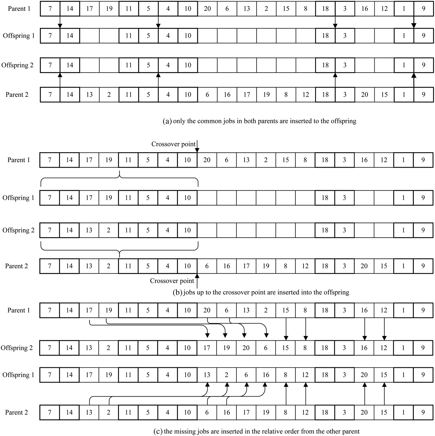
In this algorithm, we have selected similar job order crossover (SJOX; Ruiz et al., Reference Ruiz, Maroto and Alcaraz2006) and shift mutation (Ruiz et al., Reference Ruiz, Maroto and Alcaraz2006; Zobolas et al., Reference Zobolas, Tarantilis and Ioannou2009) as the reproduction operators because they performed well in preliminary experimentations. In SJOX, the job sequence from both parents is inspected individually. If both parents have same jobs in the same position, then those jobs are directly inserted into both offspring. Next, each offspring inserts all of the other jobs from one of the parents up to a random crossover point. For example, Offspring 1 directly copy jobs from Parent 1 and Offspring 2 directly copy jobs from Parent 2. Next, the missing jobs from each offspring are directly inserted from the other parent in the relative job order of that parent. For example, Offspring 1, insert the missing job from Parent 2, and for Offspring 2, insert the missing job elements from Parent 1.
Figure 2 demonstrates the process of single point SJOX. For this example, we have taken instance Ta001from Taillard's benchmark. Parent 1 and Parent 2 have makespan value 1571 and 1523, respectively. A single crossover point has been selected in between the eighth and ninth positions in the sequence. After crossover, the makespan for each offspring is 1481 and 1602, respectively.
Similar job order crossover.

In shift mutation, a job is randomly selected from the job sequence and then it is inserted into a random position in the job sequence. Each job between these two points is then moved to its adjacent position in the job sequence.
Figure 3 illustrates the shift mutation process. In this case, a job (job 10) has been randomly selected from the original schedule, and it has been inserted into another randomly selected position (17th position) in the schedule.
Shift mutation.

5.2.2. Local search
To improve the performance of the algorithm, it is common to incorporate a local search method within the GA. In this algorithm, three-stage local search methods have been applied. They include insertion neighborhood, gap filling, and a job-shifting process. The selected individuals initially go through the insertion neighbourhood search process, then through the gap filling process, and finally through job shifting.
• Insertion neighbourhood search: For solving PFSPs, insertion neighborhood performs well as a local search (Osman & Potts, Reference Osman and Potts1989; Taillard, Reference Taillard1990; Ruiz et al., Reference Ruiz, Maroto and Alcaraz2006). In this case, each job permutation has (n – 1)2 neighbors. In this process, each job is extracted from its current position and inserted into all other positions in the sequence, and if the new sequence is than the current job sequence, it then replaces the current best sequence. This process continues until all of the jobs have been evaluated.
• Gap filling: For solving PFSPs, no interjob gap is allowed when scheduling the jobs in the first machine. However due to precedence constraints, there may be some interjob gaps on all other machines. The sequence can hence be improved if these gaps can be reduced. From the preliminary experimentations, it has been observed that if in a job sequence, a gap exists in the last machine, or the last couple of machines, the sequence can often be improved by inserting a job from the right of the gap location. The process for this is as follows. Initially considering the left most gap, the total processing times for all the jobs in the sequence is calculated, and a pool of three jobs that have the least total processing time among all the jobs right of the gap are created. If a selected job is adjacent to the gap, then select the next best job from the selection pool. The total processing time of each job is the summation of its processing times in all machines. The selected job is then placed in the gap. If such a movement improves the schedule, then the new solution is accepted, and the old schedule is replaced by a new one. If not, then the job whose total processing time is the second best in the schedule is tried. The trial is limited to at most three times for each gap. After the gap identification, job selection, and insertion steps, if the makespan is improved, then the new schedules are accepted. Otherwise, move to the next gap. Finally, repeat the process for all of the gaps from left to right.
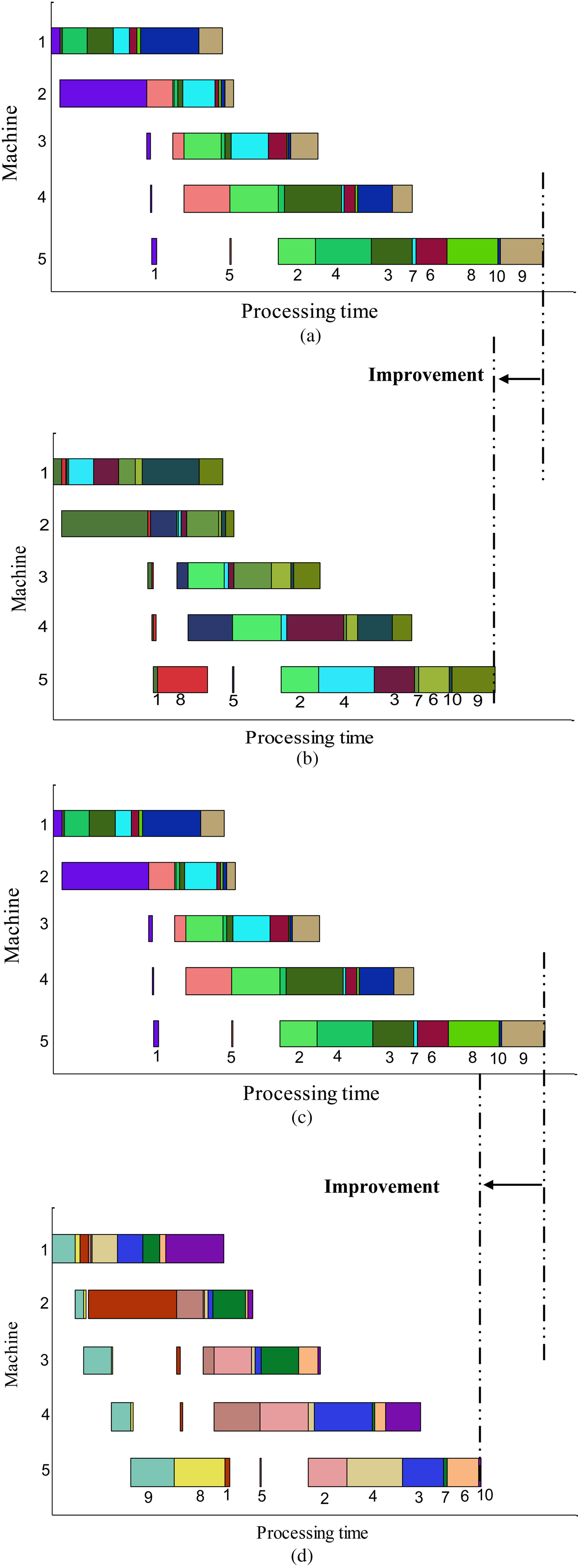
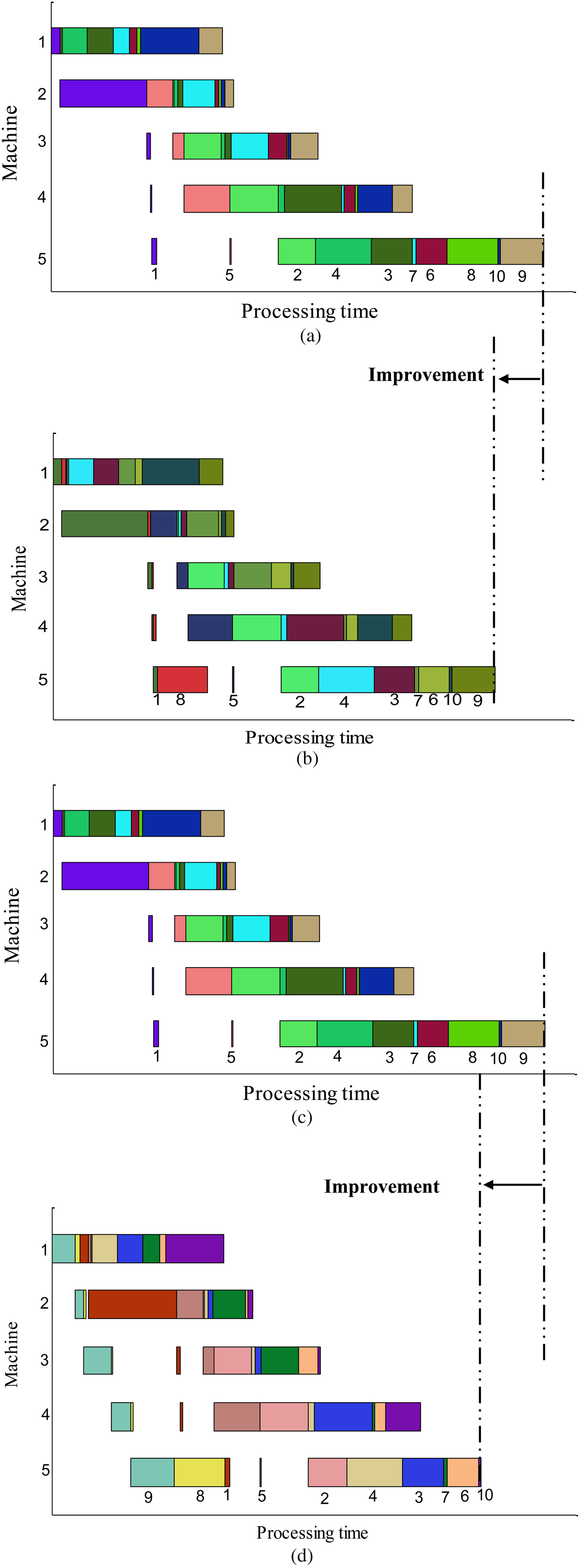
Figure 4 shows a simple illustration of the gap-filling technique. It is a five-machine, 10-job single-order flow shop. The initial job sequence is 1-5-2-4-3-7-6-8-10-9. From Figure 4a, it is clear that there is a gap between Job 1 (first job) and Job 5 (second job). In addition, this gap is the leftmost gap in the sequence. Next, a pool of 3 jobs has been selected. In this sequence, Jobs 8, 6, and 5 have the minimum total process time, respectively. However, because Job 5 is adjacent to the gap, it cannot be selected. Therefore, Job 6 is selected for the pool because it has the next lowest total processing time. Note that all these jobs from the pool are in the right of the gap. Now, if Job 8 is inserted into the gap, the solution improves (Fig. 4b). Therefore, the improved job sequence is 1-8-5-2-4-3-7-6-10-9. The improvement in schedule is indicated by the dotted line, and so the old sequence is replaced by the new one.
• Job shifting: If the jobs have longer processing time at the lower right-hand side (last few machines) of the schedule, and shorter processing time at the upper left-hand side (first or first few machines) of the job sequence, they can be moved from the right hand side to the left hand side in the schedule as much possible. The procedure is as follows: calculate the ratio of processing times (processing time in the last machine with respect to the processing time in the first machine) for all jobs in the schedule is calculated. Then, if the last three jobs in the current sequence have the bigger ratios (in this algorithm, this is limited up to three maximum ratios), then those jobs are then placed as early as possible in the sequence. A simple instance of a PFSP schedule is shown in Figure 4c. Here the eighth job (Job 8) and the ninth (last job; Job 9) are potential jobs because they have longer processing times in the last machine and smaller processing time in the first machine. Following the job-shifting rule, these jobs have been reinserted in the initial positions and these movements reduced the makespan (Fig. 4d). The new schedule is 9-8-1-5-2-4-3-7-6-10.
Fig. 4.Gap filling and job shifting techniques.

5.3. Proposed approach
In this section, the MA based right-shifting (RS) algorithm and the real-time (RT) algorithm has been presented. The proposed approach schedule or rescheduling of some or all of the accepted jobs (based on the conditions of that time) with respect to current available capacity can improve system utilization.
5.3.1. RS strategy with setup (MTO system)
In the RS approach, an order is considered as a single-order PFSP, and products from the same family may be produced in a single batch with a single setup, or be split into different batches (dynamically adjusting the batch size). The sequence of products are generated by GA based MA while using makespan minimization as the objective. Note that products are ordered by sequencing the batches from different families of products, as the same products are formed into single batches. Once the order is accepted, it starts processing in the first machine as soon as it is free. However, after processing in the first machine, if the next machine is not available immediately, the products of that order are shifted to the right. For this reason, the makespan or completion time of that order has greater value than its single-order makespan. A simple example demonstrates the overall process.
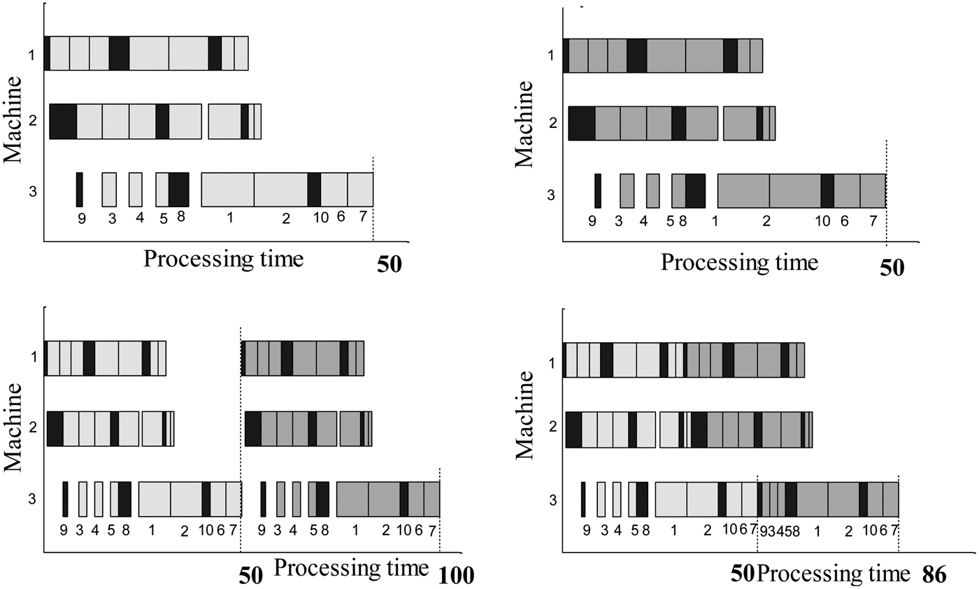
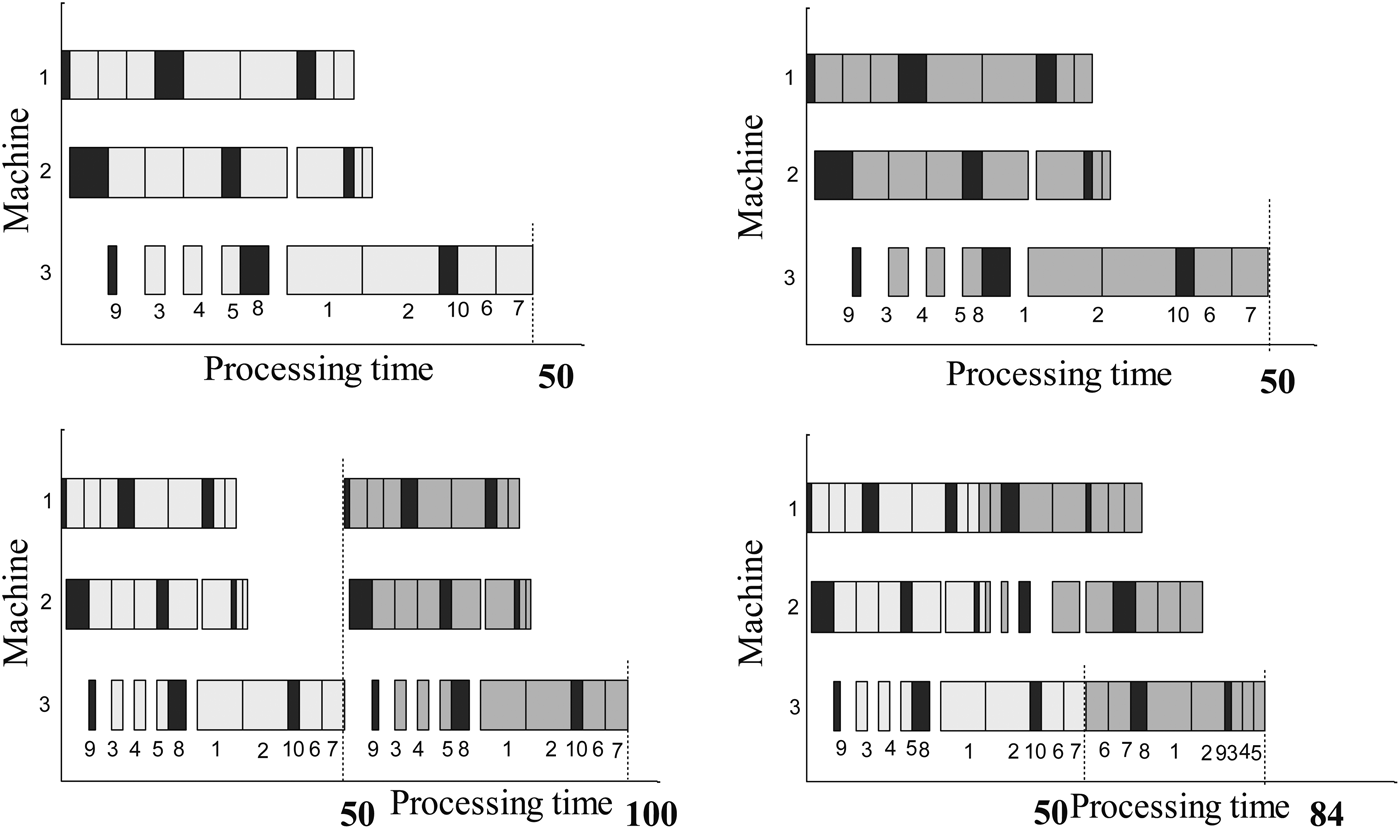
In Figure 5 we consider an instance of a three-machine flowshop problem with two orders (say, order E and F) that arrive at the production floor in two different times, and they have their own customer-specified due dates. Each order consists of seven products (say, two wash basins, three cisterns with lids, and two foot rests). In Figure 5, the black rectangular boxes represent the setup times for each product family. The Gantt chart in the upper left-hand corner presents order E, where Jobs 1 and 2 indicate two wash basins; Jobs 3, 4, and 5 indicate three cisterns with lids; and Jobs 6 and 7 indicates two footrests. The products of order E are dynamically adjusted, and the single-order makespan or completion time for order E is 50, and the sequence of products is 3-4-5-1-2-6-7. Here, Job 9 indicates the required setup times for Products 3, 4, and 5 (single setups for the products from the same family). Products 1 and 2 were processed one after another with a setup time indicated by Job 8. Similarly, Products 6 and 7 were produced within the same batch (indicated by 10). The due date for order E is 60. Therefore, this order is accepted to process in the plant.
Right-shifting strategy for Sanitaryware production.

Assume that order F arrives in the system at Time 5, when order E is still in process. Order F has the same combination of products as order E (two wash basins, three cisterns with lids, and two footrests). In the worst-case scenario, order F starts to process when order E is finished and released from the plant. In this case, the completion time of order F is 100 (in Fig. 5, the Gantt chart in the lower left-hand corner). This refers to the upper bound of the problem. However, the scenario can be improved, if after processing all the products of order E, Machine 1 immediately starts to process order F. In this case, the completion time of order F has been reduced to 86 (the Gantt chart in the lower right-hand corner). The customer set the due date for this as 90. Therefore, order F is accepted.
The algorithm with RS strategy with setup
The procedure of the RS strategy based algorithm for the MTO Sanitaryware production problem can be described as follows.
5.3.2. Algorithm 2: RS strategy for MTO PFSPs
Let the total number of orders that arrive in one production shift be L. Assume that ct is the current clock time and the due date of the lth order is d l. In addition, assume that the clock time t l, is when the first job of the lth order will start to be processed in the first, and L acpt is the number of accepted orders per production shift. The RS algorithm must then calculate the start time of the lth order, Stl, the number of product categories available in that batch, H, and the setup time required per product machine on the jth machine, s jH. The algorithm must also determine the single-order makespan of that order (C max)l, the completion time, (C comp)l, and its tardiness, T l, or its earliness, E l. Finally, the algorithm needs to calculate the profit/loss gained from the lth order, Pl, and also the total profit, P, earned from a production shift. The algorithm starts when the first customer order arrives in the production floor.
1. Set l = 1, L acpt = 0, and clock t 1 = 0
2. Continue until (l = L; up to the last order of the production shift).
A. Update the clock time, t l = ct, and Stl = ct.
B. Identify the total number of product categories from the lth product.
C. For a given product sequence, calculate the required setup time of each product by Eq. (2).
D. Use MA to find the single-order makespan of the current order.
E. Depending on the current system state, recalculate the makespan (C max)l of the current order:
a. If the lth and the (l – 1)th accepted orders are overlapping to each other, right shift the products of the lth order.
b. Else, the makespan (C max)l of the lth order is unchanged.
c. Calculate the completion time (C comp)l = Stl + (C max)l.
F. With respect to completion time, (C comp)l:
a. Calculate the tardiness/earliness, T l = (C comp)l – d l.
b. Save the completion time, (C comp)l and tardiness, T l.
c. If T l ≤ 0,
i. The lth order is Accepted.
ii. L acpt = L acpt + 1.
d. Else, the order is Rejected.
G. Calculate the profit/loss, Pl, earned from the current order.
H. Set l = l + 1.
[End of step 2 Loop]
3. Store, L acpt (total number of accepted orders in one production shift).
4. Save the total profit, P, gained from the current production shift.
[End of Algorithm]
5.3.3. RT strategy with setup (MTO system)
Once an order is placed by a customer, similarly to the RS strategy, an imaginary production schedule is generated, considering the category of products currently under process, the type of product category for which all machines are currently set up, and machine availability/unavailability constraints. On the basis of that hypothetical schedule, if the order can be processed and finished on or before its due date, it is accepted, and that brings profits to the company. Otherwise, the order is not taken.
Figure 6 demonstrates a simple example of the RT strategy. As shown in this figure, the makespan or completion time of order E is 50. Like the RS strategy, order F start to process in the first machine immediately when it completes order E. However, the schedule generated for order F considers the available production capacity at that point in time, and the status of machine setup after completing order E. Considering all these factors, the sequence of order F is 6-7-1-2-3-4-5. Note that Product 6 and 7 from order F do not need any setup because the last product (Product 7) from order E is of the same category. After scheduling order F in real time, the completion time of order F is 84 (the Gantt chart in the lower right-hand corner), which is less than the RS strategy.
Real-time strategy for Sanitaryware production.

The algorithm for RT strategy with setup
The RT strategy based algorithm, for the MTO Sanitaryware production problem, can be described as follows.
5.3.4. Algorithm 3: RT strategy for MTO PFSPs
Assume that the total number of orders that arrive in one production shift is L. The RT algorithm must then determine the start time of the lth order, Stl, the number of product categories available in that batch, H, and the setup time required per product machine on the jth machine, s jH. The algorithm must also determine the single-order makespan of that order, (C max)l, the completion time, (C comp)l, and its tardiness, T l, or its earliness, E l, and the number of accepted orders per production shift, L acpt. Finally, the algorithm calculates the profit/loss gained from the lth order, Pl, and the total profit, P, earned from a production shift.
At the beginning of a production shift, the first order arrives in the production floor and the algorithm starts.
1. Set l = 1, L acpt = 0, and clock t 1 = 0.
2. Repeat until (l < L).
A. Update the clock time, t l = ct, and Stl = ct.
B. Identify the total number of product categories in the current product.
C. For a given product sequence, calculate the required setup time of each product by Eq. (2).
D. Considering the machine availability constraints and machine setups in all machines, use MA to find a makespan of the current order.
E. Depending on the current system state, recalculate the makespan (C max)l of the current order.
F. Calculate the completion time, (C comp)l = Stl + (C max)l.
G. With respect to completion time, (C comp)l :
a. Calculate the tardiness/earliness, T l = (C comp)l – d l.
b. Save the completion time, (C comp)l and tardiness, T l.
c. If T l ≤ 0,
iii. The lth order is Accepted.
iv. L acpt = L acpt + 1.
d. Else, the order is Rejected.
H. Calculate the profit/ loss, Pl earned from the current order.
I. Set l = l + 1.
[End of step 2 Loop]
3. Store, L acpt (total number of accepted order in one production shift).
4. Save the total profit, P gained from the current production shift.
[End of Algorithm]
6. EXPERIMENTAL ANALYSIS
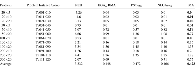
All the algorithms have been tested on small, as well as large, practical instances (20 to 200 products per order). All production data, such as processing times, setup times, order arrival times, and due dates, were collected from the practical production floor, and we have tested the proposed algorithms against 40 instances. We coded the algorithms in the C++ language, and they were run on a computer with an Intel core i7, a 2.8-GHz processor, and 4 GB RAM. In our earlier study (Rahman et al., Reference Rahman, Sarker and Essam2013), we proposed a GA based MA to solve static single-order PFSPs. The algorithm was tested against the Taillard (Reference Taillard1990) standard benchmark, and it was compared against the other competitive algorithms. These algorithms were NEH (Nawaz et al., Reference Nawaz, Enscore and Ham1983), which is both simple and the best constructive heuristics for static PFSPs; HGA_RMA (Ruiz et al., Reference Ruiz, Maroto and Alcaraz2006), which is a robust and powerful hybrid GA for static PFSPs; PSOVNS (Tasgetiren et al., Reference Tasgetiren, Liang, Sevkli and Gencyilmaz2007), which is another powerful metaheuristic algorithm that combines variable neighborhood search with a particle swarm optimization algorithm; and NEGAVNS (Zobolas et al., Reference Zobolas, Tarantilis and Ioannou2009), which is a simple and robust metaheuristic algorithm that combines with GA with different variable neighborhood search. Table 2 shows the average relative percentage of deviation (ARD) for each problem set of each of these algorithms that has been tabulated.
Comparisons between the algorithms (for single-order PFSP)
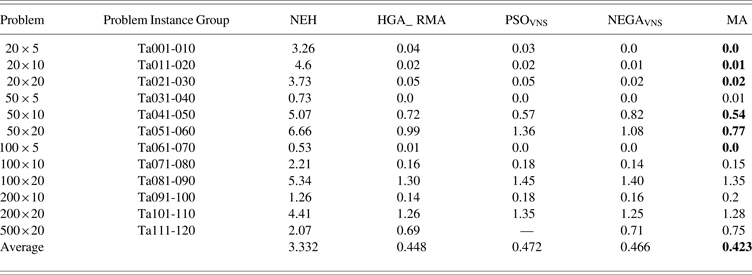
Table 2 presents the comparative results obtained by MA and other above mentioned state-of-the-art algorithms. The results in the table show the ARD between the algorithms and the so-far-determined best makespan. The first column shows the problem size (number of jobs × number of machines). The problem instances that are shown in the next column represent the problem instances, where each problem consists of 10 different problem instances. The next five columns show the average ARD (average of 10 independent runs) for each algorithm. Note that NEH (Nawaz et al., Reference Nawaz, Enscore and Ham1983) is an exception because it is a deterministic algorithm; therefore, the result for a single run has been listed. As shown in Table 2, in most problems, our algorithm outperforms the other algorithms, and also in terms of overall average (reported in the bottom row), MA shows the lowest deviation from the best known solutions.
From this computational study, it is clear that out algorithm outperforms other algorithms for solving single-order PFSPs. The reason behind addressing this computational study is the schedule generated by MA would reduce the completion time (or makespan) of each order. Therefore, the production floor may require less time to complete an order. The helps to increase the number of accepted orders by RT strategy. Therefore, our proposed MA has been extended to design a real-time strategy to solve the practical MTO PFSPs.
The combination of parameters has been based on our earlier study (Rahman et al., Reference Rahman, Sarker and Essam2013). The size of the population is set to 100. The first member in the initial population is generated from the NEH (Nawaz et al., Reference Nawaz, Enscore and Ham1983) heuristics, 40% of the members are produced from the modified NEH (Nawaz et al., Reference Nawaz, Enscore and Ham1983) heuristics, 10% of the individuals are constructed by the modified Johnson algorithm (Johnson, Reference Johnson1954), and the rest of the individuals are generated randomly. The tournament pool size is set to 5. The crossover rate is 90%, and the mutation rate is 60%. The best individual from each generation is selected as the elite, and it is preserved and passes to the next generation. If the algorithm cannot improve the solution for 10 generations, then the restart mechanism has been applied to escape from the local optimum. The local search process is applied in each generation, where the elite member and the random 29 members are selected from the current generation to go through this process.
To test the performance, we have considered three different types of scenarios: same size and combination of orders, different size but same combination of orders, and different size and combination of orders. The production plant consists of 10 machines in series. To ensure the quality and validity of the schedules generated by both the RS and RT strategies, all solutions have been compared against upper bound (UB) and lower bound (LB). The UB and LB has been derived based on the assumption that the machines or the shop may be left idle if there is no job to process. Based on these assumptions, UB and LB could be different. In this research, a reasonable one has been proposed for comparing the results.
Suppose that at time Atl an order l arrives in the production floor and also it is accepted by some manufacturing firm. In addition, assume that the completion time of order l is Ctl, and N S is the total number of accepted orders by the particular technique (as the number of accepted orders may vary for both of the strategies). If (Atl – Ctl− 1) > 0, the shops will be idle for (Atl – Ctl– 1) time period between the arrival time of order l and the completion time of order (l – 1). The positive time difference (TDl) can be defined as follows:
 $${\rm TD}^{l} = \left\{ {\matrix{{A{t}^{l} - C{t^{{l} - 1}}\comma} & {{\rm if}\,(A{t^{l}} - C{t^{{l} - 1}}) \gt 0} \cr {0\comma} & {\rm otherwise} \cr } } \right.\quad\forall \,l \ge 2.$$
UB is the worst-case scenario in completing all accepted orders. Therefore, the UB of completing N s accepted jobs can be expressed as follows:
 $${\rm UB} = \sum\limits_{l = 1}^{Ns} {C{\rm max}}^{l} + \sum\limits_{l = 2}^{Ns} {\rm TD}^l. $$
If (Atl – Ctl− 1) < 0, Machine 1 may start processing the order l as soon as it completes the order l – 1. If (Atl – Ctl− 1) < 0, the order l will require Cmaxl period of time for completing all the processes, if it starts processing just after completing order l – 1. In addition, assume that order l will arrive in the shop just after Machine 1 completes order l – 1. This situation can be the best scenario for completing all accepted N s orders. Let assume that CPtl1 is the time of completing order l on Machine 1 and Ptl1 is the total processing duration required for order l on Machine 1. Now the reduction in processing duration (RPTl) can be defined as follows:
 $${\rm RPT}^{l} = \left\{\matrix{{{C{\rm max}}^{l} - {\rm P}{\rm t}_1^l\comma} & {\hbox{if}(A{t^{l}} - C{t^{l - 1}}) \lt 0 \; \hbox{and} \ \,A{t^{l}} = \hbox{CPt}_1^{l}}\comma \cr 0 & {\rm otherwise} \cr & \qquad\qquad\qquad\forall \ge 2.} \right.$$
Therefore, the LB of completing N s accepted orders can be expressed as follows, because that is the best case scenario in completing all N s accepted orders:
 $${\rm LB} = \sum\limits_{l = 1}^{Ns} {{C{\rm max}}^{l}} - \sum\limits_{l = 2}^{Ns} {\hbox{RPT}_1^{l - 1}} + \sum\limits_{l = 2}^N {\hbox{T}{\hbox{D}^l}}. $$
The effectiveness of each method (RS or RT) can be measured by the following equations:
average deviation from the UB,
 $${D_U} = \left[\sum\limits_{l = 1}^{Ns} \left({\displaystyle{{\hbox{UB}i - Ri} \over {Ri}}} \right)\right]\Bigg/N_S\comma $$
average deviation from the LB,
 $${D_L} = \left[\sum_{l = 1}^{Ns} \left({\displaystyle{{Ri - \hbox{LB}i} \over {\hbox{LB}i}}} \right)\right]\Bigg/N_S.$$
Here Ri is the makespan of the ith accepted order achieved by MA based RS or RT.
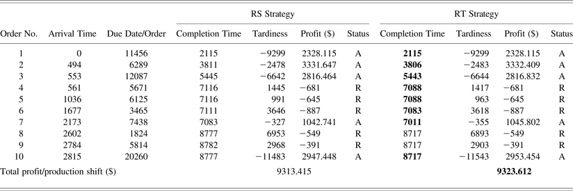
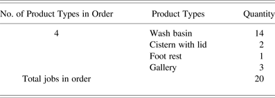
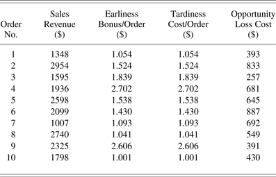
Table 3 shows the comparison between the RS and RT strategies for the 10 orders problems under Scenario 1, where all products of an accepted order must be processed on 10 machines. Each order consists of 50 products or jobs, and Table 4 shows the composition of each order. The first column represents the order number. The second and third columns present the order arrival time and due dates, respectively. These two parameters relate to current clock time, which are calculated on real time. The column headed with completion time shows the completion time of each order. The following column shows the tardiness or earliness of each order, which is calculated based on completion time and due dates. Tardiness is a prime indicator of the order acceptance/rejection decision. A negative value of tardiness means that with the available production capacity, the order can be finished on time. Otherwise, the order is tardy and there is a delay in completing the order. The column headed with profit shows the profit/loss gained from each order. Table 5 represents all costs and selling prices that relate to production.
Scenario 1 comparisons between right shifting (RS) and real time (RT) with 50 products/order

Note: A, Accepted; R, rejected.
Order composition

All relevant costs and sales revenue

At the beginning of production, the first order arrives, and after adjusting the setup on Machine 1 (adjusting the jigs, fixture, mesh size of the magnetic separator, and molds) starts to process instantly. At this point in time of production, all machines are instantly available. Therefore, the makespan and completion time (which is 2116) of this order is the same as the makespan of the single-order PFSP. The summation of the setup times and processing times of all products from the first order on Machine 1 is 1878. The arrival time of the second order is 494. Therefore, after 1878 units of time, Machine 1 starts to process the first product from the second order. Note that the last product of the first order is gallery, and after generating a hypothetical schedule with the RS strategy, the first product of the second order is wash basin. Therefore, with the RS strategy, the first product of the second order needs to set up on all machines. However, with the RT strategy, both the first product from the second order and the last product from the first order are from the same family (wash basins), and Machine 1 can start to process the first product instantly. With the RS strategy, the completion time of the second order is 3811 and the profit gain is $3331.647. In contrast, with the RT strategy, the completion time for the same order is 3806 and it earns $3332.409 profit for the company. The third order arrives in the shop while its previous orders are still in process. Therefore, the third and the second orders are overlapping, and so after acceptance, the third order is waiting in the queue and it is processed once Machine 1 is free. With both the RS and RT strategies, the fourth, fifth, and sixth orders are rejected because their completion time is greater than their due dates. Note that the seventh order arrives into the system when the third order is in process, and it starts to process while the third order is finished on Machine 1. Finally, a similar situation arises for the tenth and final order (arrives when the previously accepted order is in process in Machine 1).
The final rows reflect the total profit earned from the production shift, and show that the RT strategy based hypothetical scheduling and order acceptance decisions ensure higher profit gain than the RS strategy under this Sanitaryware production environment. Tables A.2 and A.3 in Appendix A provide the simulation results of Scenarios 2 and 3, respectively.
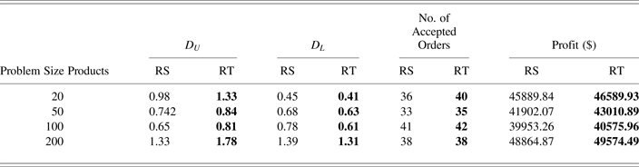
Table 6 shows a summary of comparisons between RS and RT for Scenario 1, where the same types of orders arrive into the production floor randomly. For each problem size, 10 orders with random interarrival times and due dates were generated. The table starts with a column that represents the number of products in each order.
Same order

The next two columns, headed with D U, represent the average improvement from the UB (i.e., deviation from the worst case) for RS and RT under 10 different problem instances. The following two columns represent the deviation from LB for RS and RT. In calculating LB, any violation of capacity constraints has been ignored. Note that both UB and LB have only been calculated for accepted orders. The bigger values of D U and smaller values of D L mean more improvement. In all cases, RT outperforms RS. The following two columns show the number of accepted orders by RS and RT, and the values listed in these columns show that RT is more successful in accepting more orders than the RS strategy. The last two columns show the total profit from the production shifts, and show how following the RT strategy helps to earn more profit for the company than the RS strategy.
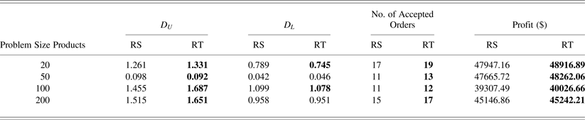
Tables 7 and 8 illustrate a comparison between RS and RT for Scenarios 2 and 3, respectively. The table representations are the same as for Table 6. For each problem instance, 25 orders with different interarrival times and due dates arrive in each production shift. For each problem size, Table 7 shows the comparison between the RS and RT strategies with respect to single problem instances. Table 8 presents a comparison between RS and RT, with respect to two independent problem instances, Cases 1 and 2. In all cases, the RT strategy performs better than the RS strategy.
Mixed order with same order size

Mixed order with different order sizes

7. CONCLUSION
This paper has presented a new approach for solving real-time multiple-order PFSPs, which was inspired from a practical Sanitaryware production problem. The problem is complex, because it requires multiple decision strategies, such as order acceptance/rejection, dynamic adjustment of setup or batch size, and scheduling the products of an order with respect to available production capacity. In the literature, very few works have addressed similar problems. To address the problem, we proposed an order acceptance heuristic and a MA based real-time algorithm. The proposed algorithms have been tested on practical production data, and the simulation results demonstrated that the proposed approach proved capable of improving the profitability of the Sanitaryware Production Company, as compared to traditional approaches.
In this research we considered the order acceptance and scheduling problem in a flowshop environment while assuming that there was no disturbance of any kind. However, in many real-world production environments, systems may be interrupted for many different reasons, such as machine breakdown, shortage of materials, and delay in supply. Future research may be carried out by extending the proposed approaches to deal with such types of interruption events.
Humyun Fuad Rahman is a Postdoctoral Research Assistant in the School of Engineering and Information Technology at the University of New South Wales, where he completed his PhD in computer science. His research mainly covers production scheduling using evolutionary algorithms. Dr. Rahman has published two high-impact journal papers and several papers in IEEE conference proceedings.
Ruhul Sarker is a Professor in the School of Engineering and Information Technology at the University of New South Wales. He received his PhD in operations research from the Department of Industrial Engineering, Dalhousie University. Dr. Sarker has published more than 230 papers in high-impact journals, edited books, and international conference proceedings. His research interests include applied operations research and evolutionary optimization.
Daryl Essam is a Senior Lecturer in the School of Engineering and Information Technology at the University of New South Wales, where he obtained his PhD in computer science. Dr. Essam's research covers design and analysis of evolutionary algorithms and optimization problem solving using evolutionary algorithms. He has published in numerous international high-impact journals and conference proceedings.
APPENDIX A
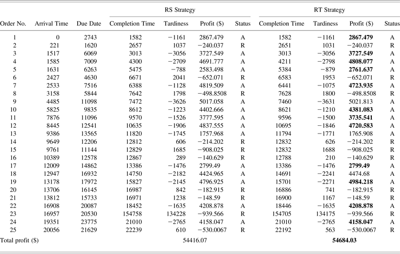
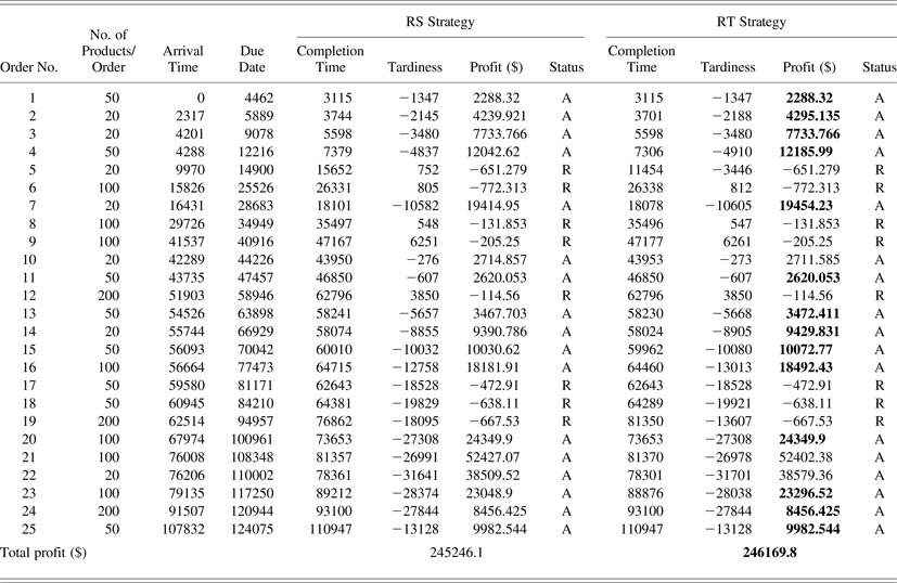
Table A.1 provides a list of raw materials. Table A.2 shows the simulation result of a sample production shift with Scenario 2 (20 products per order). In this production shift, 25 orders arrive randomly into the shop. Even though the size of each order is the same (total 20 products), the composition of each order may be different. Table A.3 presents a sample comparison between RS and RT for Scenario 3, where 25 orders arrive with different interarrival times and due dates in a production shift. Each order may be different in combination and order size.
Raw materials

Scenario 2 comparisons between right shifting (RS) and real time (RT)

Scenario 3 comparisons between right shifting (RS) and real time (RT)