1 Introduction
Diffusion flames established in the lower counterflow region of a horizontal cylindrical burner, known as Tsuji flames, have been used to study the influence of the strain rate on flame stability (Tsuji Reference Tsuji1982). Under standard conditions, in both forced and natural convection, Tsuji flames are highly stretched and, consequently, the extinction mechanism is due to the leakage of reactants by the reaction zone (Tsuji & Yamaoka Reference Tsuji and Yamaoka1967). However, under particular conditions, e.g. those found in reduced gravity environments, flames are weakly stretched and the extinction mechanism is conductive heat loss to the burner and/or radiative heat loss from the flame (Bonne Reference Bonne1971; Fernandez-Pello & Law Reference Fernandez-Pello and Law1982; T’ien Reference T’ien1986; T’ien & Foutch Reference T’ien and Foutch1987). Experimental studies of diffusion flames with very low stretch rate call for the construction of special set-ups. With a very small curvature surface, a quasi-one-dimensional counterflow is generated which achieves strain rates of approximately  $1~\text{s}^{-1}$ (Han et al. Reference Han, Ibarreta, Sung and T’ien2005). As observed, close to extinction conditions, the counterflow diffusion flame becomes transient and is broken into cells. Using the same configuration of chamber flame but with one reactant provided by a set of hypodermic needles, a one-dimensional flow is generated and the established flame becomes unstrained (Jacono et al. Reference Jacono, Papas, Matalon and Monkewitz2005). Similar behaviours as mentioned above are observed. In the first set-up mentioned above, the natural convection and the geometry of the burner are combined to impose a very low strain rate on the flame. In the second set-up mentioned above, the influence of the natural convection on the strain rate is practically removed from the region where the flame is sitting.
In the present work, a third strategy is proposed to obtain a low strain rate for buoyant Tsuji diffusion flames: reduction of the buoyant force by the increase in the ambient-atmosphere temperature. A numerical analysis quantifies the influence of the buoyant force, and by the Froude number measures its influence on the flow field and, consequently, on the flame behaviour. The present work also presents the influence of the Péclet number and the stoichiometric fuel–air ratios on the buoyant diffusion flame.
2 Configuration of the buoyancy-driven diffusion flame
The strain rate of the lower counterflow region of the buoyant Tsuji flame is determined by the fuel injection velocity and the position of the stagnation point imposed by the component of the velocity along the flame driven by the buoyancy. The proposed strategy for lowering the strain rate is to reduce the buoyancy, not through a decrease of the acceleration due to gravity but through a change of the density differences.
The buoyant force is given by  ${\hat{g}}(\hat{\unicode[STIX]{x1D70C}}_{\infty }-\hat{\unicode[STIX]{x1D70C}})$ and in the present work, the density
 $\hat{\unicode[STIX]{x1D70C}}$ satisfies
 $\hat{\unicode[STIX]{x1D70C}}_{f}\leqslant \hat{\unicode[STIX]{x1D70C}}\leqslant \hat{\unicode[STIX]{x1D70C}}_{b}$, in which
 ${\hat{g}}$ is the acceleration due to gravity and
 $\hat{\unicode[STIX]{x1D70C}}_{f}$,
 $\hat{\unicode[STIX]{x1D70C}}_{\infty }$ and
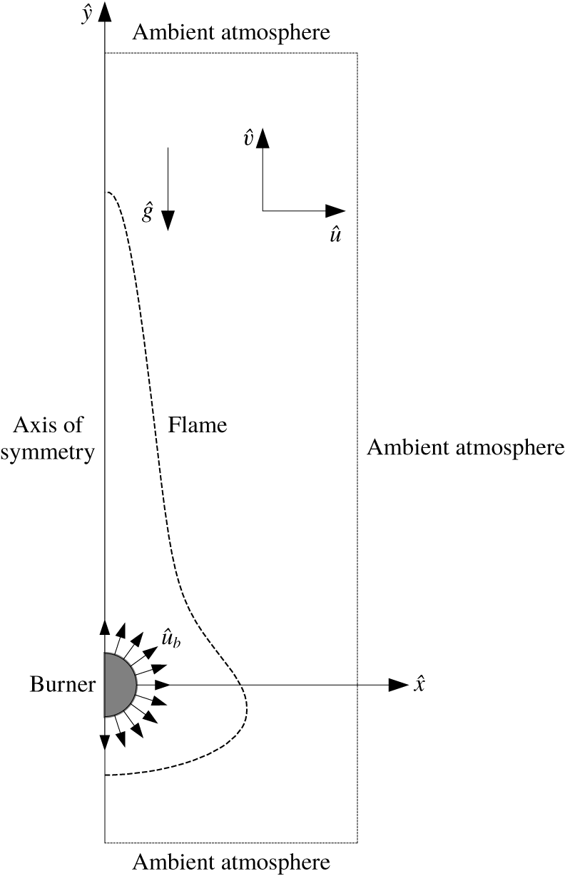
 $\hat{\unicode[STIX]{x1D70C}}_{b}$ are the density of the gases in the flame, in the ambient-atmosphere and in the burner, respectively. A schematic of the problem showing the ambient atmosphere and burner regions is exhibited in (figure 1). The conditions addressed in this analysis are such that
 $\hat{\unicode[STIX]{x1D70C}}_{f}\leqslant \hat{\unicode[STIX]{x1D70C}}_{\infty }\leqslant \hat{\unicode[STIX]{x1D70C}}_{b}$. Thus, in the region with density in the range
 $\hat{\unicode[STIX]{x1D70C}}_{f}\leqslant \hat{\unicode[STIX]{x1D70C}}\leqslant \hat{\unicode[STIX]{x1D70C}}_{\infty }$, the buoyant force is positive,
 ${\hat{g}}(\hat{\unicode[STIX]{x1D70C}}_{\infty }-\hat{\unicode[STIX]{x1D70C}})\geqslant 0$, implying that the velocity of the fluid is positive. Meanwhile, in the region with density in the range
 $\hat{\unicode[STIX]{x1D70C}}_{\infty }\leqslant \hat{\unicode[STIX]{x1D70C}}\leqslant \hat{\unicode[STIX]{x1D70C}}_{b}$, the buoyant force is negative,
 ${\hat{g}}(\hat{\unicode[STIX]{x1D70C}}_{\infty }-\hat{\unicode[STIX]{x1D70C}})\leqslant 0$, implying that the velocity of the fluid can be negative, which is the condition of the gases in the lower part of the burner. Inside the flame, the density varies from the hot gases’ density around the flame up to the cold gases’ density close to the burner, i.e.
 $\hat{\unicode[STIX]{x1D70C}}_{f}\leqslant \hat{\unicode[STIX]{x1D70C}}\leqslant \hat{\unicode[STIX]{x1D70C}}_{b}$. Outside the flame, the density varies from the hot gases’ density, around the flame, up to the cold gases’ density of the ambient atmosphere, i.e.
 $\hat{\unicode[STIX]{x1D70C}}_{f}\leqslant \hat{\unicode[STIX]{x1D70C}}\leqslant \hat{\unicode[STIX]{x1D70C}}_{\infty }$. Hence, decreasing the ambient-atmosphere density through the increase of the temperature, the difference in density
 $(\hat{\unicode[STIX]{x1D70C}}_{\infty }-\hat{\unicode[STIX]{x1D70C}}_{f})>0$ diminishes, consequently, the positive buoyancy is reduced and the result is a low upward velocity along the flame, in both sides of the flame. However, inside the flame, gases are found in the density range
 $\hat{\unicode[STIX]{x1D70C}}_{\infty }\leqslant \hat{\unicode[STIX]{x1D70C}}\leqslant \hat{\unicode[STIX]{x1D70C}}_{b}$, and, consequently, the buoyant force is negative,
 ${\hat{g}}(\hat{\unicode[STIX]{x1D70C}}_{\infty }-\hat{\unicode[STIX]{x1D70C}})<0$. Then, the cold fuel ejected from the forward part of the burner is accelerated by the action of negative buoyancy. The downward velocity of the cold fuel increases and the stagnation point is established farther from the burner.
Therefore, the increase of the ambient-atmosphere temperature leads to the reduction of the positive buoyancy of the hot gases, and to the increase of the negative buoyancy of the cold gases. The combination of these two forces by the systematic variation of the temperature of the ambient atmosphere will be used to achieve a low strain rate in the lower region of the Tsuji diffusion flame.
The rise in the ambient-atmosphere temperature not only reduces the positive buoyancy intensity and augments the negative buoyancy intensity but it also impacts their distribution. These changes in the buoyant force modify the flow field and consequently the flame properties. Unexpectedly, a drastic change is observed in the flow field in a given range of ambient atmosphere temperature. The upper vortex in the wake of the burner breaks into two. One of them is established close to the position of the primary vortex, but the other is established forward the burner.
Problem schematic (horizontal porous cylinder with fuel injection). Close to the burner, the flame presents a cylindrical geometry driven by the fuel injection, but, above the burner, a rectangular geometry driven by the buoyancy.

3 Mathematical formulation and numerical method
Diffusion flames established in a flow imposed by the fuel radial injection from a long horizontal cylindrical porous burner and by the buoyant force are analysed (figure 1). The  $\hat{x}$-component (across the flame) of the velocity
 $\hat{u}$ is a characteristic feature of natural flow field and is responsible for increasing the oxidant transport to the flame. This results in a shorter flame when compared to the one established in forced flow in which the
 $\hat{x}$-component of the velocity is negligible (Bianchin et al. Reference Bianchin, Donini, Cristaldo and Fachini2019).
In order to focus only on the combustion problem, the flow field, temperature and fuel mass fraction profile inside the burner are considered known so that the average radial velocity  $\hat{u} _{b}$, the average temperature
 $\hat{T}_{b}$ and average fuel mass fraction
 ${\hat{Y}}_{F_{b}}$ represent the conditions prevailing inside the burner.
The cylindrical burner with radius  $\hat{a}$ is in an ambient atmosphere with oxygen mass fraction
 ${\hat{Y}}_{O\infty }$, density
 $\hat{\unicode[STIX]{x1D70C}}_{\infty }$ and temperature
 $\hat{T}_{\infty }$. The subscripts
 $b$ and
 $\infty$ stand for the burner and ambient-atmosphere conditions, respectively. Since far from the burner, the flow field is driven by buoyancy, the flame exhibits a rectangular shape, as is observed in forced convection cases. However, close to the burner, the flow field is imposed by the fuel injection, then it has a cylindrical geometry. In intermediate regions, the flow field is a result of fuel injection and buoyancy, with no particular geometry. The
 ${\hat{y}}$-component (along the flame) of the velocity
 $\hat{v}$ is generated by the buoyant force.
Thermodynamic and transport coefficients, i.e. specific heat at constant pressure ( ${\hat{c}}_{p\infty }$), viscosity (
 $\hat{\unicode[STIX]{x1D707}}_{\infty }$), thermal conductivity (
 $\hat{k}_{\infty }$) and diffusion coefficient (
 $\hat{D}_{\infty }$), are considered to be constant. Both fuel and oxidant Lewis numbers are taken equal to unity. Also, an infinitely fast one-step chemical reaction is retained,
 $\text{F}+s\text{O}_{2}\rightarrow (1+s)\text{P}$, (
 $s$ mass of oxygen is consumed stoichiometrically for unit mass of fuel). Thus, the temperature
 $\hat{T}$ and the reactant mass fraction field
 ${\hat{Y}}_{i}$ (
 $i=O,~F$) are determined by two conserved functions: the mixture fraction and the excess enthalpy (Liñán Reference Liñán1991; Liñán & Williams Reference Liñán and Williams1993; Fachini Reference Fachini1999; Fachini, Liñán & Williams Reference Fachini, Liñán and Williams1999; Liñán Reference Liñán2001; Fachini Reference Fachini2007).
From the mass and momentum conservation equations, it can be inferred that the buoyancy-driven  ${\hat{y}}$-component of the velocity (along the flame) reduces the pressure along the flame. The established pressure gradient between the region of the flame and the ambient atmosphere is responsible to establish the
 $\hat{x}$-component (across the flame) of the velocity. The
 $\hat{x}$-component (across the flame) of the convective transport brings oxygen from the ambient atmosphere to close to the flame, increasing the oxygen diffusive flux to the flame. In the case of forced convection, the
 $\hat{x}$-component of the oxygen convective transport is negligible (Bianchin et al. Reference Bianchin, Donini, Cristaldo and Fachini2019). Then, in natural convection flow cases, the flame established above the cylindrical burner is narrower and shorter compared to flames in forced convection.
To investigate solely the effects of the buoyant force on the flow field, the effects of the thermal expansion on the flow field are neglected with the hypotheses of incompressible flow. To fulfil the proposed aim, density variations are only admitted in the buoyant force, which is the unique force driven by the flow field. In a compact form, the dimensionless conservation equations are
 $$\begin{eqnarray}\displaystyle & \displaystyle \unicode[STIX]{x1D6FD}^{-1}\unicode[STIX]{x2202}_{\unicode[STIX]{x1D70F}}p+\unicode[STIX]{x1D735}\boldsymbol{\cdot }\boldsymbol{u}=0, & \displaystyle\end{eqnarray}$$
 $$\begin{eqnarray}\displaystyle & \displaystyle \unicode[STIX]{x2202}_{\unicode[STIX]{x1D70F}}u+\boldsymbol{u}\boldsymbol{\cdot }\unicode[STIX]{x1D735}u=-\unicode[STIX]{x2202}_{x}p+Re^{-1}\unicode[STIX]{x1D6FB}^{2}u, & \displaystyle\end{eqnarray}$$
 $$\begin{eqnarray}\displaystyle & \displaystyle \unicode[STIX]{x2202}_{\unicode[STIX]{x1D70F}}v+\boldsymbol{u}\boldsymbol{\cdot }\unicode[STIX]{x1D735}v=-\unicode[STIX]{x2202}_{y}p+Re^{-1}\unicode[STIX]{x1D6FB}^{2}v+F_{g}, & \displaystyle\end{eqnarray}$$
 $$\begin{eqnarray}\displaystyle & \displaystyle \unicode[STIX]{x2202}_{\unicode[STIX]{x1D70F}}Z+\boldsymbol{u}\boldsymbol{\cdot }\unicode[STIX]{x1D735}Z=Pe^{-1}\unicode[STIX]{x1D6FB}^{2}Z, & \displaystyle\end{eqnarray}$$
 $$\begin{eqnarray}\displaystyle & \displaystyle \unicode[STIX]{x2202}_{\unicode[STIX]{x1D70F}}H+\boldsymbol{u}\boldsymbol{\cdot }\unicode[STIX]{x1D735}H=Pe^{-1}\unicode[STIX]{x1D6FB}^{2}H, & \displaystyle\end{eqnarray}$$
in which the flow field is determined by  $\boldsymbol{u}=(u,v)$.
The first term in (3.1) is a pseudo-transient term that appears from the artificial compressibility method and the parameter  $\unicode[STIX]{x1D6FD}$ is the artificial compressibility factor (Chorin Reference Chorin1997). The set of equations (3.1)–(3.5) achieves the steady-state solution when the pseudo-transient terms become negligible. The buoyant force (
 $F_{g}$) is considered dependent on temperature as
 $F_{g}\equiv (1-1/T)/Fr^{2}$, in which
 $Fr\,(\equiv \hat{u} _{b}/\sqrt{\hat{a}{\hat{g}}})$ is the Froude number. The isobaric approximation is used in the equation of state to implement the temperature differential in the buoyant term, which is not restricted to small density differences. The parameters
 $Re$ and
 $Pe$ are Reynolds and Péclet numbers defined as
 $Re\equiv \hat{a}\hat{u} _{b}/\hat{\unicode[STIX]{x1D708}}$ and
 $Pe\equiv \hat{a}\hat{u} _{b}/\hat{\unicode[STIX]{x1D6FC}}$ (with
 $\hat{\unicode[STIX]{x1D708}}\equiv \hat{\unicode[STIX]{x1D707}}/\hat{\unicode[STIX]{x1D70C}}_{\infty }$,
 $\hat{\unicode[STIX]{x1D6FC}}\equiv \hat{k}_{\infty }/{\hat{c}}_{p\infty }\hat{\unicode[STIX]{x1D70C}}_{\infty }$ and
 ${\hat{g}}$ the acceleration due to gravitational), respectively, based on the burner properties: fuel injection velocity and cylinder radius.
The mixture fraction is expressed as  $Z\equiv SY_{F}-Y_{O}+1$ and the excess enthalpy,
 $H\equiv (S+1)T/Q+Y_{F}+Y_{O}$, in which
 $S\equiv s{\hat{Y}}_{F_{b}}/{\hat{Y}}_{O_{\infty }}$ and
 $Q\equiv {\hat{Y}}_{F_{b}}\hat{Q}/{\hat{c}}_{p\infty }\hat{T}_{\infty }$. The choice for this definition of the mixture fraction is based on the fact that the flame is on the isoline
 $Z(x_{f},y_{f})=1$. The dependence of the flame on the fuel and its concentration are given by the field of
 $Z$,
 $0\leqslant Z\leqslant (S+1)$. The dimensionless independent and dependent variables (time, spatial coordinates, velocities, temperature and pressure) are defined as
 $\unicode[STIX]{x1D70F}\equiv \hat{\unicode[STIX]{x1D70F}}(\hat{u} _{b}/\hat{a})$,
 $x\equiv \hat{x}/\hat{a}$,
 $y\equiv {\hat{y}}/\hat{a}$,
 $u\equiv \hat{u} /\hat{u} _{b}$,
 $v\equiv \hat{v}/\hat{u} _{b}$,
 $T\equiv \hat{T}/\hat{T}_{\infty }$ and
 $p\equiv \hat{p}/\hat{\unicode[STIX]{x1D70C}}_{\infty }\hat{u} _{b}^{2}$. The fuel and oxidant mass fractions are normalized according to
 $Y_{F}\equiv {\hat{Y}}_{F}/{\hat{Y}}_{F_{b}}$ and
 $Y_{O}\equiv {\hat{Y}}_{O}/{\hat{Y}}_{O_{\infty }}$, respectively.
The independent variables are non-dimensionalized with the burner radius, but as seen in the next section, the appropriated characteristic length scales are imposed not only by the burner geometry but also by the buoyant force and the combustion process.
Equations (3.1)–(3.5) are integrated with the following boundary conditions: on the symmetry axis  $(x=0)$,
 $$\begin{eqnarray}\unicode[STIX]{x2202}_{x}u=\unicode[STIX]{x2202}_{x}v=\unicode[STIX]{x2202}_{x}p=\unicode[STIX]{x2202}_{x}Z=\unicode[STIX]{x2202}_{x}H=0;\end{eqnarray}$$
at the burner boundary surface ( $r^{2}|^{+}=x^{2}+y^{2}=1^{+}$),
 $$\begin{eqnarray}u-x=v-y=\unicode[STIX]{x2202}_{n}p=0,\quad Z_{s}-Pe^{-1}\unicode[STIX]{x2202}_{n}Z=S_{Z},\quad H_{s}-Pe^{-1}\unicode[STIX]{x2202}_{n}H=S_{H},\end{eqnarray}$$
where  $Z_{s}\equiv SY_{Fs}-1$,
 $H_{s}\equiv (S+1)T_{s}/Q+Y_{Fs}$ and the subscript
 $n$ stands for the normal coordinate (Robin’s-like boundary type for
 $Z$ and
 $H$). The terms
 $S_{Z}$ and
 $S_{H}$ are
 $Z$ and
 $H$ fluxes at the burner injection surface
 $r^{2}|^{-}=x^{2}+y^{2}=1^{-}$ as functions of
 ${\hat{Y}}_{b}$,
 $\hat{T}_{b}$ and
 $\hat{u} _{b}$, namely
 $S_{Z}\equiv S+1$ and
 $S_{H}\equiv (S+1)T_{b}/Q+1.$ Note that
 $Y_{Fs}$ and
 $T_{s}$ will be found as part of the solution of the problem.
The boundary conditions for the limits of the computational domain,  $x,|y|\rightarrow L\gg 1$ (
 $L$ is the size of the numerical domain), are
 $$\begin{eqnarray}\unicode[STIX]{x2202}_{n}u=\unicode[STIX]{x2202}_{n}v=\unicode[STIX]{x2202}_{n}p=Z=H-H_{\infty }=0,\end{eqnarray}$$
in which  $H_{\infty }\equiv (S+1)/Q+1$. According to the definition of the mixture fraction function
 $Z$, the flame position
 $(x_{f},y_{f})$ is determined by the isoline
 $Z(x,y)=1$. The subscript
 $f$ stands for flame condition. On the isoline
 $Z=1$, the flame temperature
 $T_{f}$ is determined by
 $H(x_{f},y_{f})=(S+1)T_{f}/Q$.
The governing equations, equations (3.1)–(3.5), are discretized by the quadratic upstream interpolation for convective kinetics (known as QUICK) scheme to guarantee stability, sensitivity to the flow direction and third-order truncation error (Fletcher Reference Fletcher2012). The steady-state solution for (3.1)–(3.5) is achieved with an artificial time integration using the second-order Runge–Kutta Ralston method.
Computation difficulties arise from the lack of an explicit equation for pressure. To avoid them, a treatment based on the artificial compressibility method is used to couple pressure and velocity fields leading to (3.1) (Chorin Reference Chorin1997). A bidimensional stretched structured staggered grid is adopted to avoid fluctuating pressure distributions. We considered a mass fraction of methane inside the burner equal to  ${\hat{Y}}_{F_{b}}=0.5$. The aim of this value is to shorten the flame height, and so to reduce the extension of the computational domain.
4 Analysis of order of magnitude
Tsuji diffusion flames around a cylindrical porous burner considering natural convection are quite similar to those established considering forced convection. In the latter case, the  $x$-component (across the flame) of the convective transport is negligible. However, in the former case, oxygen is transported by convection from the ambient atmosphere to near the flame, which imposes a higher oxygen flux to the flame. Therefore, the fuel consumption is also augmented and, consequently, the flame dimensions are reduced. To have a fundamental comprehension of Tsuji diffusion flames under the influence of natural convection, the characteristic spatial and velocity scales imposed by the buoyant force, fuel injection and combustion are determined.
The orders of magnitude of the flame width  $L_{x}\,(\equiv \hat{L}_{x}/\hat{a})$, flame height
 $L_{y}\,(\equiv \hat{L}_{y}/\hat{a})$, variation of velocity in the
 $x$-direction
 $U\,(\equiv \hat{u} _{\infty }/\hat{u} _{b})$ and variation of velocity in the
 $y$-direction
 $V\,(\equiv \hat{v}_{\infty }/\hat{u} _{b})$ are defined. Where the order of magnitude
 $L_{x}$ is set at
 $y=L_{y}/e$ and
 $L_{y}$ at the flame tip,
 $x=0$. The characteristic velocities driven by the buoyancy are defined by
 $(\hat{u} _{\infty },\hat{v}_{\infty })$. From the mass conservation, the following relation is found:
 $U/L_{x}\sim V/L_{y}$.
Balancing inertia and buoyant force terms in the  $y$-component of the Navier–Stokes equation, the second and last terms of (3.3), one finds the relation
 $V^{2}/L_{y}=\unicode[STIX]{x1D6E5}^{2}/(Fr)^{2}$, in which
 $\unicode[STIX]{x1D6E5}^{2}\equiv 1-1/T_{f}$. In the same way, balancing the inertia and viscous terms of the Navier–Stokes equation, the second and the fourth terms of (3.3), a third relation among the properties is obtained,
 $U=1/PeL_{x}$. In the order of magnitude analysis, the approximation
 $Re=Pe$ is justified.
The fourth relation, necessary to close the system, is the flame width found in the Tsuji flame established by forced convection,  $L_{x}=(S+1)Pe^{-1/4}V^{-3/4}$ (Bianchin et al. Reference Bianchin, Donini, Cristaldo and Fachini2019). Although the flame width
 $L_{x}$ is not explicitly dependent on the
 $x$-component of the velocity
 $U$, its dependence is through the
 $y$-component of the velocity
 $V$.
Then, the scales of the problem can be specified as a function of the Froude ( $Fr$) and Péclet (
 $Pe$) numbers, the expansion parameter (
 $\unicode[STIX]{x1D6E5}$) and the combustion parameter (
 $S$) according to
 $$\begin{eqnarray}\displaystyle & \displaystyle L_{x}=Pe^{-2/5}(\unicode[STIX]{x1D6E5}/Fr)^{-3/5}(S+1)^{2/5}, & \displaystyle\end{eqnarray}$$
 $$\begin{eqnarray}\displaystyle & \displaystyle L_{y}=Pe^{2/5}(\unicode[STIX]{x1D6E5}/Fr)^{-2/5}(S+1)^{8/5}, & \displaystyle\end{eqnarray}$$
 $$\begin{eqnarray}\displaystyle & \displaystyle U=Pe^{-3/5}(\unicode[STIX]{x1D6E5}/Fr)^{3/5}(S+1)^{-2/5}, & \displaystyle\end{eqnarray}$$
 $$\begin{eqnarray}\displaystyle & \displaystyle V=Pe^{1/5}(\unicode[STIX]{x1D6E5}/Fr)^{4/5}(S+1)^{4/5}. & \displaystyle\end{eqnarray}$$
Note that, since the Péclet number is based on the burner properties, it determines qualitatively the effect of the fuel injection from the cylindrical burner on the flow field and on the flame. In the same way, the term  $\unicode[STIX]{x1D6E5}/Fr$ quantifies the effect of buoyancy on the flow field and on the flame, while the
 $(S+1)$ term measures qualitatively the effect of the combustion process on the flow field. This simple analysis reveals also the dependence of the flame length on
 $S$, which is not as strong as in the forced convection case because of the oxidant flux across the flame.
The set of equations (4.1)–(4.4) is also consistent with the known behaviour of the flame observed (i) in the microgravity regime  $\unicode[STIX]{x1D6E5}/Fr\rightarrow 0$ (Qian & Law Reference Qian and Law1997), where
 $(L_{x},L_{y}\rightarrow \infty )$ and (ii) in the forced convection regime where the velocity component
 $V$ is vanishing (Bianchin et al. Reference Bianchin, Donini, Cristaldo and Fachini2019).
5 Discussion
The cases presented and commented on in this section are chosen to highlight the processes controlling the diffusion flame established around a horizontal cylindrical burner with a buoyancy-driven flow. In all cases,  $\hat{a}$ and
 $\hat{u} _{b}$ are chosen to satisfy
 $Re\leqslant 30$, preventing any type of instabilities of the flame above the burner.
The temperature distribution exhibited in the figures is in dimensional form to facilitate the comparison between the plots. Since the dimensional temperature of the ambient atmosphere changes from case to case, the burner temperature is fixed and the flame temperature varies slightly among the cases, then, it was decided to present the dimensional temperature in the figures which leads to a minimal number of modifications from case to case. In all cases the burner temperature is  $\hat{T}_{b}=300K$ and the fuel is methane.
5.1 Influence of  $\unicode[STIX]{x1D6E5}/Fr$, $Pe$ and $S$ on the flame


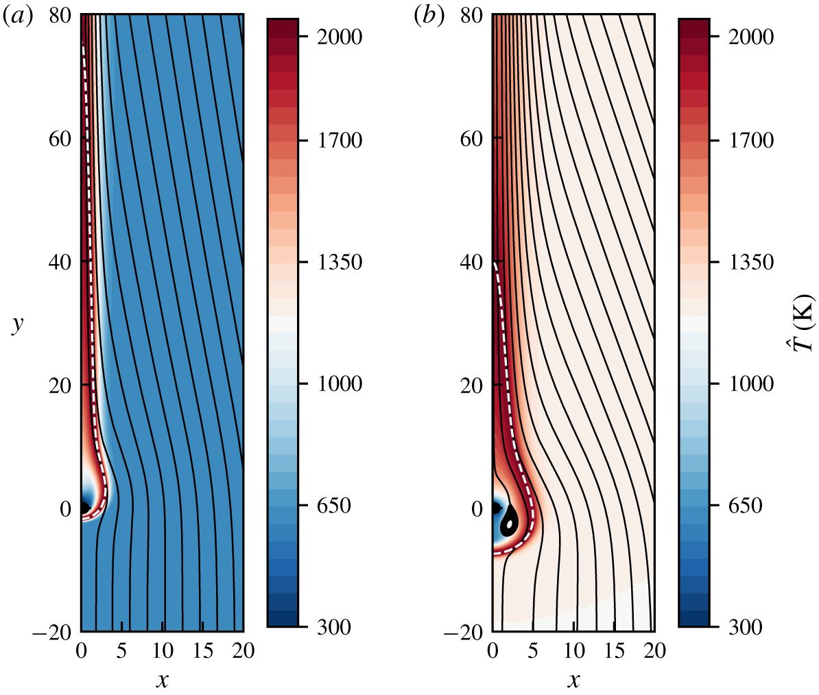
The colourmap contour shows the temperature distribution and the dashed line shows the flame shape for different ambient temperatures: (a)  $\hat{T}_{\infty }=2\hat{T}_{b}$ (
 $1/T_{b}=2$,
 $Pe=7.83$,
 $Fr=1$,
 $\unicode[STIX]{x1D6E5}=0.84$) and (b)
 $\hat{T}_{\infty }=4\hat{T}_{b}$ (
 $1/T_{b}=4$,
 $Pe=3.6$,
 $Fr=1$,
 $\unicode[STIX]{x1D6E5}=0.63$). The cylindrical burner is represented here by the black area at the origin
 $(x,y)=(0,0)$.

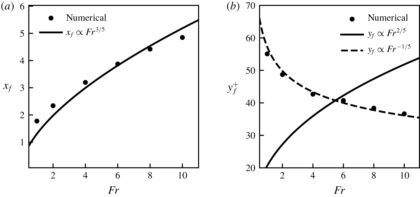
(a) Flame width  $x_{f}$ at
 $y=y_{f}^{+}/e$ and (b) flame height
 $y_{f}^{+}$ as functions of the Froude number, for
 $\hat{T}_{\infty }=3\hat{T}_{b}$,
 $Pe=5.2$,
 $\unicode[STIX]{x1D6E5}=0.74$,
 $S=9.5$.

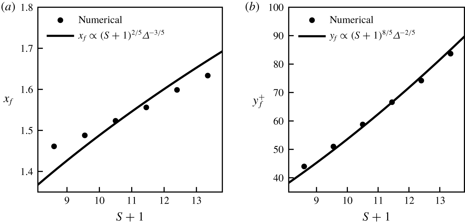
Figure 2 presents the behaviour of the whole flame with reduction in the buoyancy through reduction in the density difference in the buoyant force,  $(1-\unicode[STIX]{x1D70C})/Fr^{2}$, imposed by the increase of the ambient-atmosphere temperature.
From an analysis of (4.1)–(4.4), it is seen that a decrease of the buoyancy term  $\unicode[STIX]{x1D6E5}/Fr$ through an ambient-atmosphere temperature rise leads to a reduction of the velocity components
 $(U,V)$. The consequence of this is a decrease of the oxygen and fuel convective fluxes to the flame. The decrease of the oxygen convective flux, which is almost perpendicular to the flame, forces the flame to move away from the symmetry axis, i.e. the flame width increases. This behaviour is correctly captured by the expression for
 $L_{x}$, equation (4.1), and confirmed by the numerical results shown in figure 3(a). However, the same arguments cannot be used to describe the effects of the reduction of fuel convective transport on the length of the flame
 $L_{y}$. Since the fuel convective transport occurs mainly along the flame, its reduction results in a shortening of the flame associated with the fuel concentration decrease inside the flame. The proof of this conclusion is given by the dependency of the fuel flux on buoyancy. From (4.1) to (4.4), it is seen that the fuel convective transport in a cross-section of the flame diminishes with the reduction of the buoyancy according to
 $L_{y}\sim L_{x}V\sim (\unicode[STIX]{x1D6E5}/Fr)^{-1/5}$. As in jet flames, the fuel convective transport in the
 $y$ direction determines the flame length, those results are confirmed by the numerical results presented in figure 3(b).
It is worth noticing that the expression for the flame length  $L_{y}\sim (\unicode[STIX]{x1D6E5}/Fr)^{-2/5}$, given by (4.2), does not capture the flame shortening driven by the decrease of the buoyancy in the addressed conditions. Contrarily, the flame length increases with the reduction of the buoyancy. This behaviour is found for a vanishing buoyant force (Qian & Law Reference Qian and Law1997) and in forced convection Tsuji flames with incoming velocity approaching zero (Bianchin et al. Reference Bianchin, Donini, Cristaldo and Fachini2019). Therefore, combining these two behaviours, it is possible to deduce that the reduction of the buoyancy initially shortens the flame length because of the decrease in the
 $y$-component of the fuel convective transport. After that, the reduction in the buoyancy extends the flame length because the
 $y$-component of the fuel’s diffusive and convective transport become of the same order. In such a condition, both processes control the behaviour of the flame in the
 $y$ direction. The condition
 $L_{y}\sim L_{x}$ (or from the mass conservation
 $V\sim U$) reflects the above statement and is derived from
 $(\unicode[STIX]{x1D6E5}/Fr)\sim [Pe^{4}(S+1)^{6}]^{-1}\ll 1$. Taking this result into (3.3) and rescaling the time, spatial dimensions and velocity, it is seen that the transient period would be of the order of
 $\unicode[STIX]{x1D70F}_{c}\sim (\unicode[STIX]{x1D6E5}/Fr)^{-2}=[Pe^{4}(S+1)^{6}]^{2}\gg 1$, the characteristic spatial dimensions of the flame would be
 $(x_{c},y_{c})\sim (\unicode[STIX]{x1D6E5}/Fr)^{-1}=[Pe^{4}(S+1)^{6}]\gg 1$ and the characteristic velocity imposed by fuel injection and buoyancy would be
 $(u_{c},v_{c})\sim (\unicode[STIX]{x1D6E5}/Fr)=[Pe^{4}(S+1)^{6}]^{-1}\ll 1$.
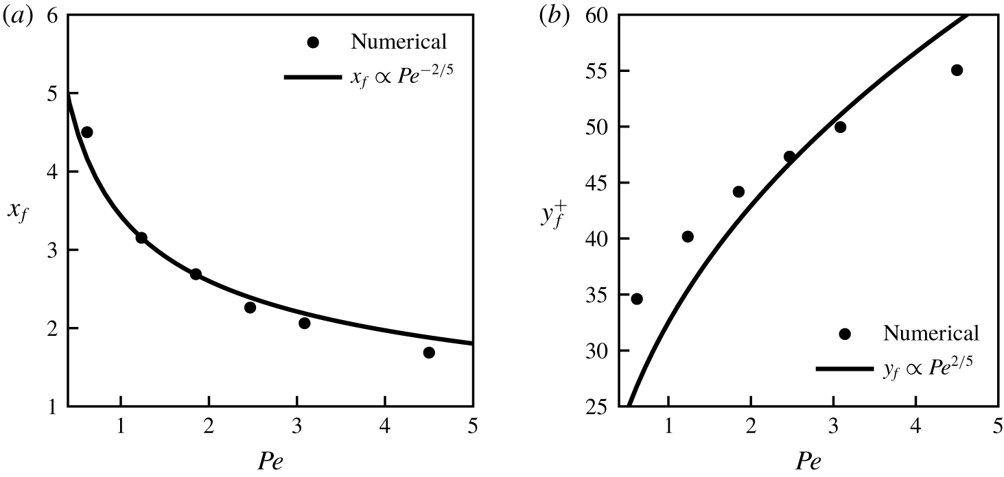
(a) Flame width  $x_{f}$ at
 $y=y_{f}^{+}/e$ and (b) flame height
 $y_{f}^{+}$ as functions of the Péclet number, for
 $\hat{T}_{\infty }=3\hat{T}_{b}$,
 $Fr=1$,
 $\unicode[STIX]{x1D6E5}=0.74$,
 $S=9.5$.

Figure (4) exhibits the behaviour of the flame dimensions (width and length) in terms of Péclet number  $Pe$. The results from the order of magnitude analysis for the flame width
 $x_{f}\sim Pe^{-2/5}$ and flame height
 $y_{f}^{+}\sim Pe^{2/5}$ are in line with the trend observed in the numerical results, as seen in plots figure 4(a,b). An increase in the Péclet number means that more fuel mass is injected by augmenting the velocity of injection and/or the surface area of the burner. The injection of more fuel leads to a longer flame for burning the fuel, as seen in figure 4(b). The elongated flame represents buoyant force acting over a large distance which increases the velocity along the flame as
 $V\sim Pe^{1/5}$. However, as in forced convection Tsuji flames (Bianchin et al. Reference Bianchin, Donini, Cristaldo and Fachini2019), the increase on the
 $y$-component of the velocity reduces the flame width, as depicted in figure 4(a).
(a) Flame width  $x_{f}$ at
 $y=y_{f}^{+}/e$ and (b) flame height
 $Y_{F}$ as functions of the combustion parameter
 $S$, for
 $\hat{T}_{\infty }=3\hat{T}_{b}$,
 $Fr=1$,
 $Pe=4.5$,
 $0.735\leqslant \unicode[STIX]{x1D6E5}\leqslant 0.748$.

Figure 5 shows the dependence of the width and length of the flame on the combustion parameter  $S$. Since
 $S$ influences the flame temperature, and hence the expansion parameter
 $\unicode[STIX]{x1D6E5}$, then the behaviour of the flame width and length are compared with
 $\unicode[STIX]{x1D6E5}^{-3/5}(S+1)^{2/5}$ and
 $\unicode[STIX]{x1D6E5}^{-2/5}(S+1)^{8/5}$, respectively. As seen in both plots, figure 5(a,b), an increase in the fuel concentration of the fuel stream injected at the burner demands the flame dimensions become larger for burning stoichiometrically the additional amount of fuel.
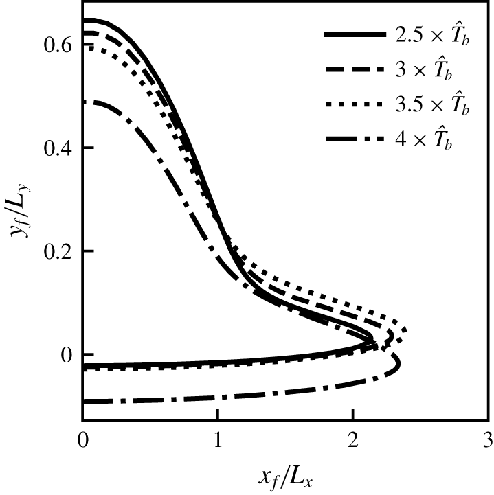
Figure 6 shows the whole rescaled flame for four ambient-atmosphere temperatures  $\hat{T}_{\infty }=(2.5,3,3.5,4)\times \hat{T}_{b}$ and all of them present practically the same dimensions. The concordance of these dimensions confirm that the spatial scales
 $L_{x}$ and
 $L_{y}$ are the proper scales to study flames established around a Tsuji burner. As can be easily noted, the flame shape for the case
 $1/T_{b}\equiv \hat{T}_{\infty }/\hat{T}_{b}=4$ is displaced downward. The reason for that is the establishment of a second recirculation zone (second vortex) below the burner. The presence of this vortex changes substantially the flow field close to the burner and the flame as consequence. The discussion of the flow field under several ambient-atmosphere conditions is presented in detail below.
Rescaled flame coordinates  $y_{f}/L_{x}$ and
 $x_{f}/L_{y}$ for several values of the ambient-atmosphere temperatures
 $\hat{T}_{\infty }=2.5\hat{T}_{b}$,
 $3\hat{T}_{b}$,
 $3.5\hat{T}_{b}$,
 $4\hat{T}_{b}$. The values of the parameters are
 $Fr=1$,
 $S=9.5$,
 $Pe=5.93$, 5.2, 4.35, 3.6 and
 $\unicode[STIX]{x1D6E5}=0.79$, 0.74, 0.68, 0.63, respectively.

5.2 Influence of the ambient-atmosphere temperature on the flow field
The flow field above the burner is controlled only by the positive buoyancy of the hot gases. Under this force, the flow field can be described as parallel and is accelerated, like the flow field found in jet flames, as seen in figure 2. However, the flow field changes drastically around (above and below) the burner. The combination of the positively buoyant hot gases (around the flame) and the negatively buoyant cold gases’ (around the burner) buoyancy and the fuel injection imposes a different flow field morphology. This flow field resembles the one imposed by a forced flow around a cylinder, from which fluid is injected backward and forward in the direction of the forced flow (Sen, Mukhopadhyay & Sen Reference Sen, Mukhopadhyay and Sen2017).
The focus of this section is on the processes controlling the flow field around the burner, in which the forward counterflow (Tsuji) diffusion flame is established. As proposed in this analysis, the conditions of low strain rate for the Tsuji flame are sought.
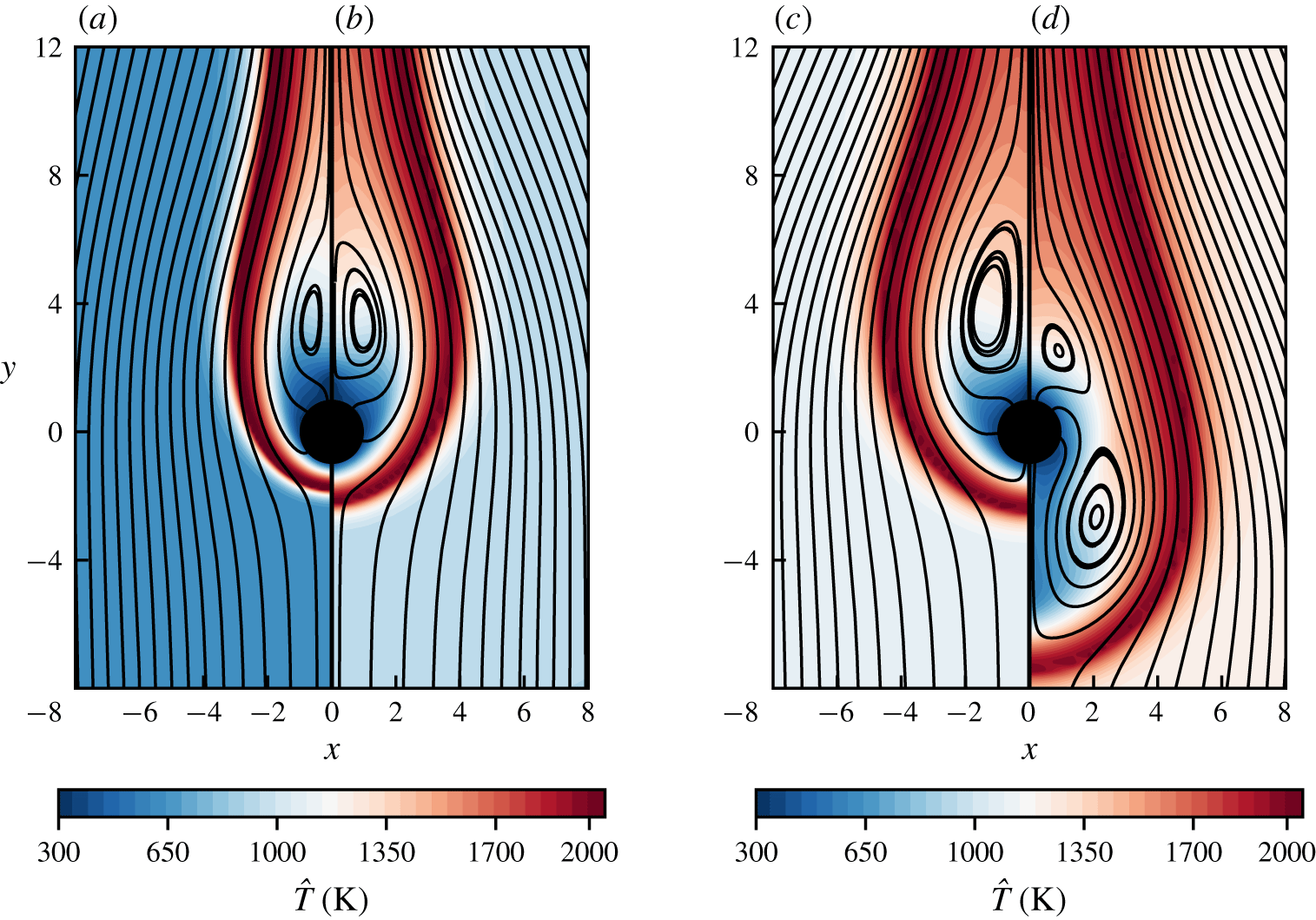
The plots show the streamlines and the temperature contours for different ambient temperatures: (a)  $\hat{T}_{\infty }=2\hat{T}_{b}$ (
 $Pe=7.83$,
 $Fr=1$,
 $\unicode[STIX]{x1D6E5}=0.84$), (b)
 $3\hat{T}_{b}$ (
 $Pe=5.2$,
 $Fr=1$,
 $\unicode[STIX]{x1D6E5}=0.74$), (c)
 $3.5\hat{T}_{b}$ (
 $Pe=4.35$,
 $Fr=1$,
 $\unicode[STIX]{x1D6E5}=0.68$) and (d)
 $4\hat{T}_{b}$ (
 $Pe=3.6$,
 $Fr=1$,
 $\unicode[STIX]{x1D6E5}=0.63$). The colour scale contour shows the dimensional temperature distribution for all cases.

Figure 7 presents the flow field and the temperature distribution close to the burner. In that region, the recirculation zones are established. For ambient-atmosphere temperatures such that  $\hat{T}_{\infty }=2\hat{T}_{b}$,
 $3\hat{T}_{b}$ and
 $3.5\hat{T}_{b}$ (figure 7a–c) the positive buoyant force overwhelms the negative one, even close to the burner. In this scenario, the positive
 $y$-component of velocity is high enough to maintain the recirculation zone above the burner, as well as the counterflow region close to the bottom side of the cylinder. The vortex above the burner is established at a certain distance from the burner because of the fuel injection. Unlike the recirculation zone generated in the forced convection regime whose width is of the order of the cylinder radius, in the present analysis, the vortex width depends not only on the burner radius but also on the flame width, in which the buoyant force accelerates the flow. Since the flame width increases with the reduction in the buoyant force, then the vortex becomes wider as buoyancy is reduced.
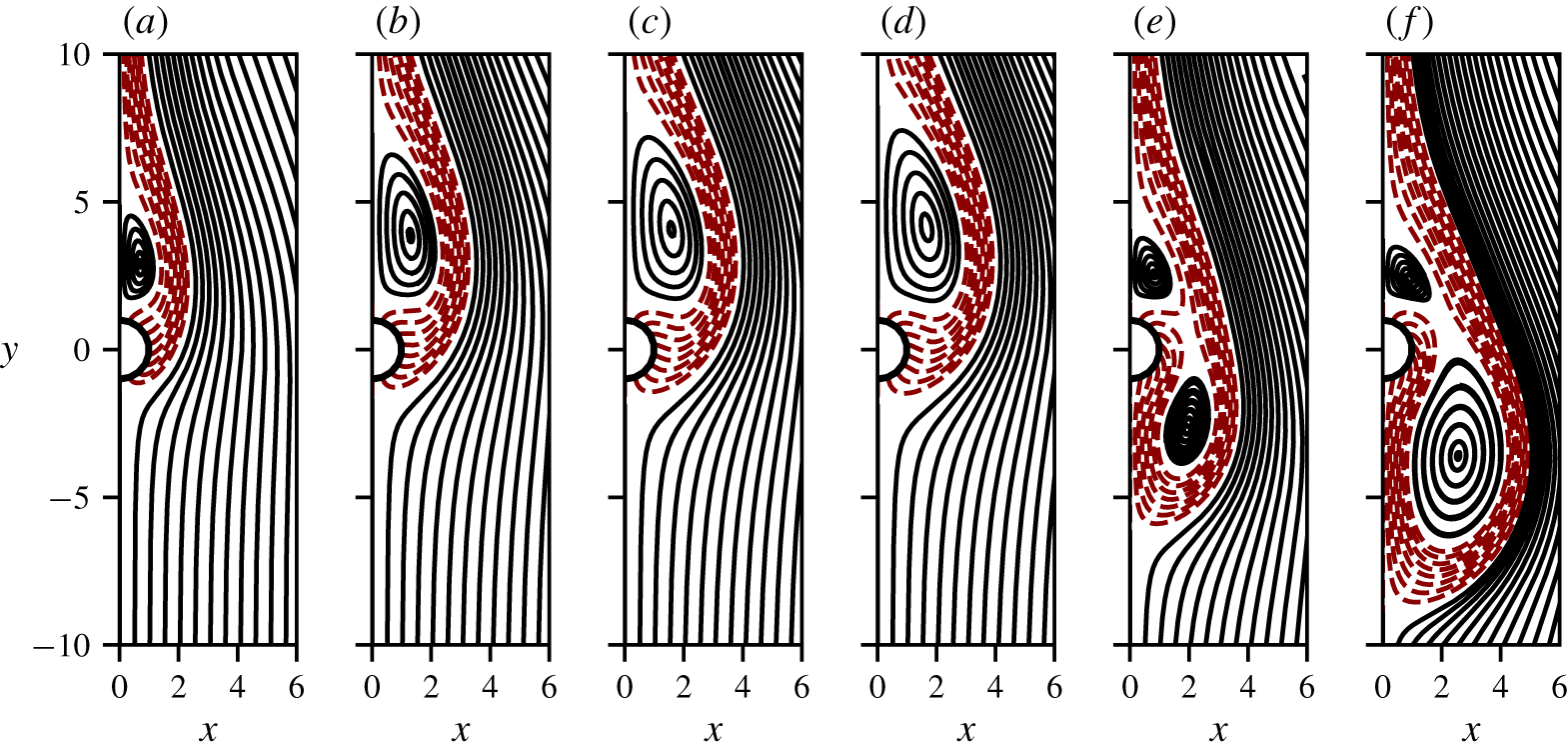
Streamlines for different ambient-atmosphere temperatures: (a)  $\hat{T}_{\infty }=2.5\hat{T}_{b}$, (b)
 $3.5\hat{T}_{b}$, (c)
 $3.8\hat{T}_{b}$, (d)
 $3.89\hat{T}_{b}$, (e)
 $3.895\hat{T}_{b}$ and (f)
 $4.5\hat{T}_{b}$.

The backward recirculation zone is due to an adverse pressure gradient generated by the buoyancy-driven flow field, which is imposed by the presence of the flame. The flow field close to the burner is comparable to the flow past a cylinder with vortex shedding control through the blowing of the cylinder surface (Li et al. Reference Li, Navon, Hussaini and Le Dimet2003). The major difference between them though is the  $x$-component of velocity generated by the buoyancy, which is responsible for keeping the vortex inside the fuel zone steady in the wake, preventing the occurrence of a vortex shedding. These changes in the flow field and temperature distribution are proportional to the variation of the ambient-atmosphere temperature.
As seen in figure 7(d), the flow field changes dramatically for an ambient-atmosphere temperature  $1/T_{b}=\hat{T}_{\infty }/\hat{T}_{b}=4$. An additional recirculation zone can be observed below the burner, approximately
 $y=-4$ . This new recirculation zone modifies completely the flow field, which changes the flame shape and consequently the temperature distribution and the buoyant force field. The conditions addressed in that case are such that the negative buoyant force of the cold fuel, surrounding the cylindrical burner, overcomes the positive one, which imposes a negative
 $y$-component of velocity. In addition to that, the region in which negative buoyancy is found increases drastically, as shown by the blue region of figure 7(d). The consequences are a wider flame and a stagnation point pushed away from the burner.
Therefore, the increase of the ambient-atmosphere temperature has two opposing effects: a reduction of the positive buoyancy and an increase of the negative one. The latter drives the cold fuel increasingly downwards below the burner, creating a cold gas pocket which deviates the inflow. The consequence is a wider flame.
The dramatic impact of the increase of the ambient-atmosphere temperature on the flow field is evident in figure 8. The switch between a one-vortex to a two-vortex configuration is observed when  $\hat{T}_{\infty }$ exceeds a critical value of
 $3.895\hat{T}_{b}$. Below that value, the one-vortex configuration prevails (figure 8a,d) with a stand-alone upper vortex whose size is an increasing function of
 $\hat{T}_{\infty }$ and whose location is slightly shifted away from the cylinder as
 $\hat{T}_{\infty }$ increases. Above the critical value of
 $\hat{T}_{\infty }$, the two-vortex configuration takes over (figure 8e,f). The change of the patterns of the streamlines originating from the injection surface of the burner (red colour and dashed lines) is clearly visible. This is caused by the fact that the negative buoyant force overwhelms the positive one. As a consequence, the descending cold gases and the ascending hot gases are energetic enough to create a circular anticlockwise motion corresponding to the observed lower vortex. It is worth mentioning the pattern of the streamlines in the recirculation zone does not represent the mass flow rate.
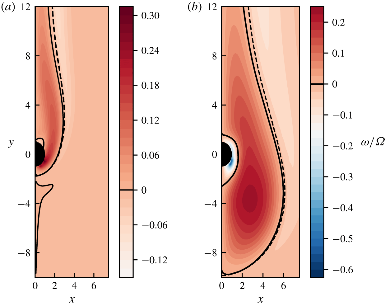
Flame shape (dashed line) and non-dimensional vorticity contour, scaled by  $\unicode[STIX]{x1D6FA}=V/L_{x}-U/L_{y}$, for different ambient temperatures: (a)
 $\hat{T}_{\infty }=2\hat{T}_{b}$ (
 $Pe=7.83$,
 $\unicode[STIX]{x1D6E5}=0.84$) and (b)
 $\hat{T}_{\infty }=4.5\hat{T}_{b}$ (
 $Pe=3$,
 $\unicode[STIX]{x1D6E5}=0.58$). The colourmap contour shows the vorticity
 $\unicode[STIX]{x1D714}/\unicode[STIX]{x1D6FA}$ distribution and the continuous line represents the isocontour of
 $\unicode[STIX]{x1D714}/\unicode[STIX]{x1D6FA}=0$.

As a consequence of the one- and two-vortex configurations, the combustion-driven buoyancy creates two vortical structures close to the burner, as shown in figure 9. The first structure presented by figure 9(a) is quite similar to the configuration of a non-reactive flow past a cylinder without injection (Fornberg Reference Fornberg1980). The vortex is found in the wake of the burner as the one-vortex configuration, but the maximum positive vorticity value is situated close to the surface of the burner where the injected fuel is highly deflected by the positive buoyant force.
As seen in figure 9(b), the second vortical structure appears due to the two-vortex configuration with high vorticity driven by the pair of negative and positive buoyant forces below the burner, which create a large vortex in the fuel-containing region, centred at  $(x,y)=(3,-4)$. Increasing the ambient-atmosphere temperature, not only increases the intensity of the negative buoyant force but also the extension of the region in which this force is found. Therefore, the vorticity is spread below the burner in a large region of the flow. This lower vortical structure is similar to that found in a non-reactive flow past a cylinder, from which fluid is injected and aligned with the free stream flow (Sen et al. Reference Sen, Mukhopadhyay and Sen2017). However, in that configuration the upstream vortex is unstable, i.e. the vortex position initially oscillates and after that is completely detached from the cylinder. On the other hand, the buoyancy-driven vortical structure analysed in the present work remains close to the cylinder, inside the fuel region and enclosed by the flame.
To quantify the overall effect of the ambient-atmosphere temperature  $\hat{T}_{\infty }$ on the vorticity, it is defined the following vorticity integral:
 $$\begin{eqnarray}\unicode[STIX]{x1D714}_{T}=\int _{-L}^{L}\left(\int _{0}^{x_{f}(y)}|\unicode[STIX]{x1D714}|\,\text{d}x\right)\text{d}y,\end{eqnarray}$$
over the fuel-containing region (limited by the dashed line). The dimensionless vorticity  $\unicode[STIX]{x1D714}$ is
 $\unicode[STIX]{x1D714}=\unicode[STIX]{x2202}_{x}v-\unicode[STIX]{x2202}_{y}u$, and its integral
 $\unicode[STIX]{x1D714}_{T}$ is named as the total vorticity. This definition captures not only the changes of the vorticity intensity but also the changes on the extension of the flame, as can be seen in two cases exhibited in figure 9. The total vorticity varies from
 $\unicode[STIX]{x1D714}_{T}=2.16$ to
 $\unicode[STIX]{x1D714}_{T}=16$, for
 $\hat{T}_{\infty }=2\hat{T}_{b}$ and
 $4.5\hat{T}_{b}$, respectively.
Also, figure 9 reveals that the vorticity is well scaled by the properties found in the order of magnitude analysis, i.e.  $\unicode[STIX]{x1D6FA}=V/L_{x}-U/L_{y}$. Since
 $L_{y}\gg L_{x}$ and
 $V\gg U$, then the estimate of the vorticity can be written as
 $\unicode[STIX]{x1D6FA}=V/L_{x}$, which reveals the dependence of the vorticity on the problem parameters
 $\unicode[STIX]{x1D6FA}=Pe^{3/5}(\unicode[STIX]{x1D6E5}/Fr)^{7/5}(S+1)^{2/5}$.
5.3 Influence of the ambient-atmosphere temperature on the strain rate
In appendix A, an estimate of the strain rate in the lower part of the Tsuji flame is obtained as a function of the Froude number  $Fr$, temperature of burner, ambient atmosphere and flame, along with the position of the flame, according to (A 7). Writing it in dimensional form, one finds
 $$\begin{eqnarray}\left.\frac{\text{d}\hat{v}}{\text{d}{\hat{y}}}\right|_{y_{f}^{-}}\sim \frac{\unicode[STIX]{x1D6E5}^{2}}{v_{f}}\frac{{\hat{g}}}{\hat{u} _{b}}.\end{eqnarray}$$
The expression for the estimate of the strain rate echoes the main idea of the present work, i.e. diminishing the strain rate by increasing the ambient-atmosphere temperature, such that  $\unicode[STIX]{x1D6E5}^{2}$ decreases while the velocity in the flow increases.
As presented in appendix A, for the ambient-atmosphere temperature  $\hat{T}_{\infty ,c}=(\hat{T}_{f}-\hat{T}_{b})/\ln (\hat{T}_{f}/\hat{T}_{b})$, the velocity at the flame is
 $v_{f}=1$, then the strain rate is estimated as
 $$\begin{eqnarray}\left.\frac{\text{d}\hat{v}}{\text{d}{\hat{y}}}\right|_{y_{f}^{-}}\sim \frac{{\hat{g}}}{\hat{u} _{b}}\frac{\hat{T}_{f}-\hat{T}_{\infty ,c}}{\hat{T}_{f}}.\end{eqnarray}$$
For the cases in which  $\hat{T}_{\infty }>\hat{T}_{\infty ,c}$, the velocity
 $v_{f}>1$, then strain rate decreases
 $$\begin{eqnarray}\left.\frac{\text{d}\hat{v}}{\text{d}{\hat{y}}}\right|_{y_{f}^{-}}<\frac{{\hat{g}}}{\hat{u} _{b}}\frac{\hat{T}_{f}-\hat{T}_{\infty ,c}}{\hat{T}_{f}}.\end{eqnarray}$$
For instance, for  $Fr=1$,
 $S=9.5$,
 $\hat{T}_{b}=300K$ and
 $\hat{T}_{\infty }=1200K$, the flame temperature is
 $\hat{T}_{f}=2050K$, the flame position is
 $y_{f}^{-}=-7.4$ (numerical), the velocity at the flame
 $v(y_{f}^{-})$ is
 $(0.12,1.74)$ (numerical and (A 6), respectively), the stagnation point
 $y_{st}$ is
 $(-6.72,-4.29)$ (numerical and (A 4), respectively) and the dimensionless strain rate is
 $(0.1125,0.2383)$ (numerical and (A 7), respectively).
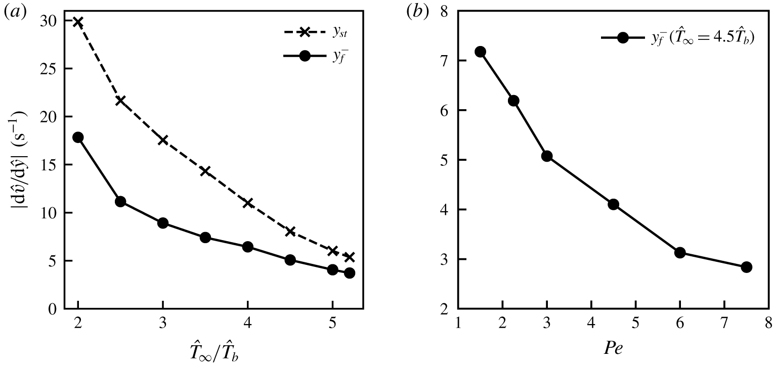
(a) Strain rate at the flame  $y_{f}^{-}$ and at the stagnation point
 $y_{st}$ on the negative
 $y$ axis as a function of several ambient-atmosphere temperatures:
 $\hat{T}_{\infty }=(2,2.5,3,3.5,4,4.5,5,5.2)\hat{T}_{b}$, for which
 $Pe=7.83$, 5.93, 5.2, 3.6, 3, 2.22, 2.1 and
 $\unicode[STIX]{x1D6E5}=0.84$, 0.79, 0.74, 0.68, 0.63, 0.58, 0.52, 0.5, respectively. (b) Strain rate at the flame
 $y_{f}^{-}$ as a function of Péclet number. For all cases,
 $\hat{T}_{\infty }=4.5\hat{T}_{b}$,
 $Fr=1$ and
 $S=9.5$ are considered.

The strain rate of the lower stagnation flow around the symmetry axis is influenced by the buoyancy-driven flow. With the increase of the ambient-atmosphere temperature, the positive buoyancy decreases and the buoyancy-driven flow has a lower  $y$-component of the velocity, which results in lower counterflow flames with a low strain rate. Increasing the ambient temperature from
 $2$ times to
 $5.2$ times the burner temperature, the strain rate on the lower counterflow diffusion flame reduces from
 $16~\text{s}^{-1}$ to
 $3.5~\text{s}^{-1}$ (see figure 10a). As indicated by (5.1), choosing an ambient temperature of
 $\hat{T}_{\infty }=4.5\hat{T}_{b}$ and changing the Péclet number by an increase of
 $\hat{u} _{b}$, further reduction on the strain rate is achieved, with a minimum value of
 $2.8~\text{s}^{-1}$, as shown in figure 10(b).
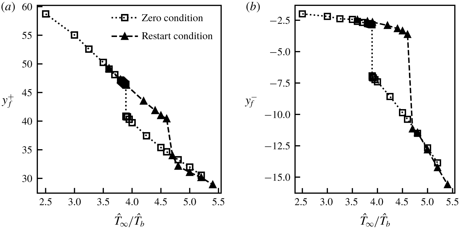
(a) Flame tip  $y_{f}^{+}$ and (b) flame bottom
 $y_{f}^{-}$ as a function of the ratio of ambient-atmosphere temperature to burner temperature
 $\hat{T}_{\infty }/\hat{T}_{b}$ (
 $Fr=1$,
 $S=9.5$).

5.4 Dependence of the steady solution on the initial condition
As shown in figure 8(d,e), with changes of the ambient-atmosphere temperature, the flow field changes drastically. Moreover, as shown in figure 11, with changes of the initial conditions, the flow field becomes unexpectedly sensitive to the initial conditions in a certain range of ambient-atmosphere temperature. The two limits of the flame on the  $y$ coordinate (flame tip
 $y_{f}^{+}$ and bottom
 $y_{f}^{-}$) are used to quantify the effects of the ambient-atmosphere temperature as well as the initial conditions on the steady solution, as seen in figures 11(a) and 11(b), respectively.
Two configurations of initial conditions are considered. The first one is a cylindrical flame starting close to the burner with a uniform flow field, named as the zero condition. The second one is a known solution for a different ambient-atmosphere temperature, named as the restart condition. If the ambient-atmosphere temperature of the known solution, used as an initial condition, is close to the one of the searched new solutions, the simulations can be seen as a continuous change on the far field conditions. Using these two types of initial conditions, a jump on the steady solution is identified, but not in the same ambient-atmosphere temperature, according to figure 11. The jump in the solutions shows the strong nonlinearity of the problem and jumps for different ambient-atmosphere temperatures for different initial conditions reveal a hysteresis of the steady solutions.
The results show no dependency on the initial conditions in the ranges  $2.5\leqslant \hat{T}_{\infty }/\hat{T}_{b}\leqslant 3.89$ and
 $4.6<\hat{T}_{\infty }/\hat{T}_{b}\leqslant 5.2$. In the first range, the positive buoyancy overwhelms the negative one everywhere and the presence of the burner imposes the establishment of a vortex in the wake of the burner, as discussed previously. In the second range, the negative buoyancy overwhelms the positive one below the burner and a second vortex is established in this region, as discussed previously. However, the balance between the positive and negative buoyancy below the burner for
 $3.8925\leqslant \hat{T}_{\infty }/\hat{T}_{b}\leqslant 4.6$ and the geometric factor imposed by the burner as an immersed body lead to the dependency of the solution on the type of the initial conditions, as exhibited in figure 11(a,b).
The drastic change on the solutions at the ambient-atmosphere temperature  $\hat{T}_{\infty }/\hat{T}_{b}=4.6$ occurs when the negative buoyancy overwhelms the positive one and vice versa at the ambient-atmosphere temperatures
 $\hat{T}_{\infty }/\hat{T}_{b}=3.8925$. For the former case, the cold flow pushes the flame further away from the burner. The descending cold gases flow from the burner and the ascending hot gases flow around the flame create a second recirculation zone (vortex) forward the burner. Once the flow field with two vortices is established, a large decrease of the negative buoyancy is necessary for the flow to return to its previous state (i.e. the flame close to the burner, and only one vortex is found with its location in the burner wake). The condition for the return is found in the latter case, i.e.
 $\hat{T}_{\infty }/\hat{T}_{b}=3.8925$. The different behaviour of the steady solutions for the two initial conditions used in the analysed range of ambient-atmosphere temperature
 $2.5\leqslant \hat{T}_{\infty }/\hat{T}_{b}\leqslant 5.2$ shows the hysteresis of the buoyancy-driven Tsuji diffusion flame.
6 Conclusion
The aim of the present numerical analysis was to investigate the possibility of reduction of the strain rate in Tsuji flames by varying the temperature of the ambient atmosphere. The model considers the thermal expansion only in the buoyant force term of the Navier–Stokes equations. The variation of the ambient-atmosphere temperature modifies simultaneously the positive buoyancy of the hot gases and the negative buoyancy of the cold gases. Then, the reduction of the effects of the buoyancy on the whole flame established around the horizontal cylindrical porous burner is achieved by a proper combination of those two forces. For the cases in which the positive buoyancy overwhelms the negative buoyancy, the lower part of the Tsuji flame is close to the burner, the length of the upper part of the flame is approximately two orders of magnitude of the burner radius. In the flow field, there is one vortex in the wake of the burner. For the cases in which the negative buoyancy overwhelms the positive buoyancy, the lower part of the flame is farther from the burner, and the length of the upper part of the flame is reduced considerably. The flow field changes drastically because, besides the vortex in the burner wake, a second vortex is established below the burner. The systematic increase in the ambient-atmosphere temperature modifies not only the intensity of the buoyant forces but also the domain in which each of them is found. Because of the change in these two properties with the ambient-atmosphere temperature, the transition of the negative buoyancy overwhelming the positive buoyancy and vice versa are discontinuous. Moreover, since the flow fields for these two conditions are very different, then the ambient-atmosphere temperatures for the transitions are not the same. This behaviour causes a hysteresis on the buoyancy-driven Tsuji diffusion flame. The numerical results point out that the strategy of increasing the ambient-atmosphere temperature leads to low-strain-rate Tsuji diffusion flames.
Acknowledgements
We thank Dr Pascal Bruel (CNRS, Pau, France) for helpful discussions, and the financial support provided by CAPES and CNPq (grants 1698503, 1700552, 302717/2016-1) is greatly acknowledged.
Declaration of interests
The authors report no conflict of interest.
Appendix A. Stagnation point and strain rate estimation
Considering a fluid particle, determined by  $y_{p}$, leaving the downside surface of the burner and displacing downwards on the symmetry axis, the force balance equation for determining its trajectory is given by
 $$\begin{eqnarray}\frac{\text{d}^{2}y_{p}}{\text{d}t^{2}}=\frac{1}{Fr^{2}}\left(1-\frac{1}{T}\right).\end{eqnarray}$$
Diffusion flames established in a counterflow configuration are known to sit in the oxidant side at a distance from the stagnation plane which scales as  $Pe^{-1/2}$, thus, the flame position can be estimated by
 $y_{f}^{-}\sim y_{st}-Pe^{-1/2}$.
In this analysis, a linear temperature profile from the burner up to the flame is imposed, i.e.  $T\sim T_{b}+\unicode[STIX]{x1D6E5}_{T}(y_{p}+1)$, with
 $\unicode[STIX]{x1D6E5}_{T}=(T_{f}-T_{b})/(y_{f}^{-}+1)$.
Multiplying (A 1) by  $2\,\text{d}y_{p}/\text{d}t$ and integrating analytically, the fluid velocity on the symmetry axis below the burner is determined by
 $$\begin{eqnarray}(Fr^{2})\left(\frac{\text{d}}{\text{d}t}(y_{p}+1)\right)^{2}=2(y_{p}+1)-\frac{2}{\unicode[STIX]{x1D6E5}_{T}}\ln \left(1+\frac{\unicode[STIX]{x1D6E5}_{T}(y_{p}+1)}{T_{b}}\right)+(Fr^{2})\end{eqnarray}$$
in which the boundary condition at the burner surface was applied, i.e.  $v=y_{p}^{\prime }=-1$ at
 $y_{p}=-1$. The position of the stagnation point
 $y_{p}=y_{st}$ is found with the zero velocity condition
 $y_{p}^{\prime }=0$,
 $$\begin{eqnarray}\frac{(y_{st}+1)}{(y_{f}^{-}+1)}+\frac{(Fr)^{2}}{2(y_{f}^{-}+1)}=\frac{1}{(T_{f}-T_{b})}\ln \left(1+\frac{(T_{f}-T_{b})}{T_{b}}\frac{(y_{st}+1)}{(y_{f}^{-}+1)}\right).\end{eqnarray}$$
A way to find the solution of (A 3) is made in two steps. First, the position  $y_{tan}$ at which the functions of the left- and right-hand sides have the same tangent is calculated. Second, the condition for
 $(Fr)^{2}/2(y_{f}^{-}+1)$ that makes the two functions meet at
 $y_{tan}$ is determined. Following this strategy, the stagnation point is determined by
 $$\begin{eqnarray}(y_{st}+1)=\frac{1-T_{b}}{T_{f}-T_{b}}(y_{f}^{-}+1)\end{eqnarray}$$
and the Froude number is
 $$\begin{eqnarray}\frac{(Fr)^{2}}{2(y_{f}^{-}+1)}=\frac{\ln (1/T_{b})+T_{b}-1}{T_{f}-T_{b}}.\end{eqnarray}$$
Imposing the flame position  $y_{p}=y_{f}^{-}$ into (A 2), the velocity
 $v_{f}=v(y_{f}^{-})$ can be estimated by
 $$\begin{eqnarray}(v_{f}-1)(v_{f}+1)=\frac{|y_{f}^{-}+1|}{(Fr)^{2}}\left(\frac{\ln (T_{f}/T_{b})}{T_{f}-T_{b}}-1\right).\end{eqnarray}$$
From (A 6), the velocity of the gases at the flame is independent of the flame position for the particular ambient-atmosphere temperature  $\hat{T}_{\infty ,c}=(\hat{T}_{f}-\hat{T}_{b})/\ln (\hat{T}_{f}/\hat{T}_{b})$ and its value is
 $v_{f}=1$. The velocity is positive because the flame is in the oxidant side of the counterflow. For the addressed conditions,
 $\hat{T}_{b}=300K$ and
 $S=9.5$, which leads to
 $\hat{T}_{f}=2050K$ and
 $\hat{T}_{\infty ,c}$ is
 $910K$. For
 $\hat{T}_{\infty }>910K$, the velocity is
 $v_{f}>1$.
The strain rate at the flame  $y_{f}^{-}$ is estimated by the derivative in
 $y$ direction of (A 6), according to
 $$\begin{eqnarray}\left.\frac{\text{d}v}{\text{d}y_{p}}\right|_{y_{f}^{-}}=\frac{\unicode[STIX]{x1D6E5}^{2}}{(Fr)^{2}v_{f}},\end{eqnarray}$$
which reveals its dependence on the Froude number and on the temperature of the flame, the fuel injected and the ambient atmosphere. For instance,
 $$\begin{eqnarray}\left.\frac{\text{d}v}{\text{d}y_{p}}\right|_{y_{f}^{-}}\left[\begin{array}{@{}c@{}}{>}\\ =\\ {<}\end{array}\right]\Big(\frac{\unicode[STIX]{x1D6E5}}{Fr}\Big)^{2},\quad \text{for }\left\{\begin{array}{@{}c@{}}\hat{T}_{\infty }<\hat{T}_{\infty ,c}\,(v_{f}<1)\\ \hat{T}_{\infty }=\hat{T}_{\infty ,c}\,(v_{f}=1)\\ \hat{T}_{\infty }>\hat{T}_{\infty ,c}\,(v_{f}>1).\end{array}\right.\end{eqnarray}$$