1. Introduction
Blasius (Reference Blasius1908) showed that the velocity profile in a laminar boundary layer over a flat plate has a similar shape at all streamwise distances from the leading edge of the plate when the non-dimensional parameter
 ${\it\eta}=y\sqrt{U_{1}/{\it\nu}x}$
(
 $U_{1}$
is the free-stream velocity,
 ${\it\nu}$
is the kinematic viscosity of the fluid and
 $x$
is the streamwise distance) is introduced. In this case, the boundary layer can be described as self-preserving. In general, self-preservation (SP) implies that the equations governing the flow admit similarity solutions based on only one velocity scale and one length scale. If a turbulent boundary layer is in SP state (often referred to as ‘equilibrium’ turbulent boundary layer), quantities such as the mean velocity and Reynolds stresses should not evolve with
 $x$
when normalised by these SP scales. A considerable number of attempts were made in the past (e.g., Clauser Reference Clauser1954, Reference Clauser1956; Townsend Reference Townsend1956, Reference Townsend1976; Rotta Reference Rotta1962) to determine the required conditions for an equilibrium turbulent boundary layer. Clauser (Reference Clauser1954, Reference Clauser1956) recognised that a zero pressure gradient (ZPG) turbulent boundary layer cannot be in a SP. He stated further (Clauser Reference Clauser1954) that the velocity profile of a ZPG turbulent boundary layer over a rough wall presents a greater lack of similarity than on a smooth wall. This latter statement has been proved to be incorrect. He also identified a class of simple equilibrium flows which he associated with a constant value of the parameter
 ${\it\beta}=({\it\delta}^{\ast }/{\it\tau}_{w})(\text{d}p/\text{d}x)$
, where
 ${\it\delta}^{\ast }$
is the displacement thickness,
 ${\it\tau}_{w}$
is the wall shear stress and
 $\text{d}p/\text{d}x$
is the mean streamwise pressure gradient. Mellor & Gibson (Reference Mellor and Gibson1966) extended the work of Clauser and Townsend and showed that the defect velocity profile of a smooth-wall turbulent boundary layer is in equilibrium for a range
 $-0.5\leqslant {\it\beta}\leqslant \infty$
.
In searching for SP conditions of a ZPG turbulent boundary layer, Townsend (Reference Townsend1956, Reference Townsend1976) and Rotta (Reference Rotta1962) realised that the viscous effects near the wall preclude the boundary layer from growing in a self-similar manner, and confined their analysis to the outer region of the boundary layer, where the viscous effects are assumed to be negligible. In other words, both Townsend (Reference Townsend1956, Reference Townsend1976) and Rotta (Reference Rotta1962) have carried out a SP analysis by omitting the viscous term in the mean momentum equation. Townsend (Reference Townsend1956) recognised that, unless the variation of the wall shear stress in
 $x$
is negligible, at least two velocity scales are needed to describe the turbulent boundary layer. He commented that dividing the boundary layer into inner and outer layers, each with their own scales of length and velocity, relaxes certain SP conditions. However, in order to determine the inner and outer scales of the two-layer model, one must apply order of magnitude estimates of each term in the equations of motion. At this stage, it is important to note that Townsend (Reference Townsend1956) emphasised that the two-layer model is an approximation, which is only valid if the differences in scales are not too great. He then argued that one can use the results obtained by assuming full SP (i.e. across the entire layer) to estimate the differences between the scales of the two layers. This has led to an alternative approach for studying the self-similarity of a turbulent boundary layer, i.e. asymptotic analysis. In other words, the governing equations are studied under the condition that
 $Re$
is very large, in which case the viscous term has a negligible effect on the boundary layer (except in the very near-wall region). Most notably, George & Castillo (Reference George and Castillo1997) used the asymptotic invariance principle (AIP) of George (Reference George1995) and suggested that the free-stream velocity (
 $U_{1}$
) is the correct velocity scale by asserting that it leads to a similarity solution of the mean momentum equation in the outer region. It should be remarked that in addition to the viscous term, the turbulent diffusion term in the governing equation of the mean momentum is neglected in the analysis of George & Castillo (Reference George and Castillo1997), who argued, based on the results of Tennekes & Lumley (Reference Tennekes and Lumley1972), that this term vanished at infinite
 $Re$
. Later, Jones, Nickels & Marusic (Reference Jones, Nickels and Marusic2008) pointed out, again via asymptotic arguments, that
 $U_{{\it\tau}}$
is an equally valid velocity scale. This non-uniqueness of scaling parameters is a result of making certain assumptions about the governing equations, e.g. considering only the outer region, or analysing the equations under some special constraints, e.g.
 $Re\rightarrow \infty$
. The review of Gad-el Hak & Bandyopadhyay (Reference Gad-el Hak and Bandyopadhyay1994) is particularly relevant to the issue discussed here. They compared the magnitude of Coles wake parameter
 ${\it\Pi}$
(Coles Reference Coles1956) in experimental data over a large range of
 $Re$
and found that
 ${\it\Pi}$
does not reach a constant value. Based on this argument, Gad-el Hak & Bandyopadhyay (Reference Gad-el Hak and Bandyopadhyay1994) concluded that it would not be possible to achieve self-preservation in a smooth-wall ZPG turbulent boundary layer.
The lack of self-similarity in a smooth-wall turbulent boundary layer has led to the concept of scaling analysis (SA), which regards finding a length scale and a velocity scale leading to collapse of the normalised mean turbulence quantities. This is usually done via dimensional analysis, empirical methods, asymptotic and order of magnitude arguments. Although, both SP and SA aim to find scaling parameters, they are fundamentally quite different. SA relies on certain assumptions about the governing equations (e.g. the mean momentum equation for a turbulent boundary layer), or experimental data over a finite range of
 $Re$
, and hence the scaling parameters are not uniquely determined. In other words, one does not strictly adhere to the SP constraints in SA, which leads to non-universal scaling parameters. One may cite the classical example of a laminar boundary layer over a flat plate. SA leads to correct scaling parameters but only because it is confirmed by SP and ultimately by an exact (Blasius Reference Blasius1908) solution of the Navier–Stokes equations. For a turbulent boundary layer, where the two-layer model has been invariably used, SA has led to non-rigorous results for the inner region and probably also the outer region. This has led to ‘incomplete similarity’ laws for the mean velocity distribution in a turbulent boundary layer (see Barenblatt Reference Barenblatt1993, Reference Barenblatt1996, for example). A good illustration of this difficulty is the lack of consensus between the log-law and the power-law. Barenblatt (Reference Barenblatt1993) showed that both log-law and power-law formulations for the mean velocity profile in the overlap region (a region common to the inner and outer layers) can be derived using dimensional arguments but based on different physical assumptions, viz. whether or not the velocity gradient is completely independent of viscosity.
Further, as is amply evident in the literature, SA has led to a variety of scaling parameters. For instance, Zagarola & Smits (Reference Zagarola and Smits1998) discussed that the ratio of outer and inner velocity scales must approach a constant value at very large
 $Re$
and proposed
 $U_{1}{\it\delta}^{\ast }/{\it\delta}$
as the outer velocity scale (
 ${\it\delta}$
and
 ${\it\delta}^{\ast }$
are the boundary layer thickness and displacement thickness, respectively). Similarly, a wide range of length scales have been suggested aside from the conventional inner length scale (
 ${\it\nu}/U_{{\it\tau}}$
) and the outer length scale (
 ${\it\delta}$
). To mention a few, Rotta (Reference Rotta1962) used dimensional arguments to replace
 ${\it\delta}$
by
 $U_{1}{\it\delta}^{\ast }/U_{{\it\tau}}$
and Weyburne (Reference Weyburne2008) reasoned that
 ${\it\delta}^{\ast }$
is the correct length scale based on the requirement that the areas under all the scaled velocity profiles in a self-preserving flow must be equal.
So far, there has been no rigorous SP analysis carried out on a rough-wall turbulent boundary layer equation including the form drag caused by the roughness elements. Rotta (Reference Rotta1962) discussed SP for a turbulent boundary layer over a rough wall. However, his analysis was similar to that carried out for a smooth wall. He considered the mean momentum equation without the viscous term to study the region away from the wall where the viscous effects are negligible and he used an empirical argument for introducing the roughness height
 $k$
as a scaling parameter into the analysis. He found that
 $k$
must increase in proportion to
 $x$
. In the present work, we apply a SP analysis on a turbulent boundary layer equation which includes the form drag when the boundary layer develops on a rough surface. We show that the approach allows us to demonstrate in a rigorous manner that
 $k$
must vary linearly with
 $x$
but does not require to be introduced empirically as a scaling parameter.
The paper is organised as follows. In § 2, we derive the SP conditions on the basis of the mean momentum equation without making a priori assumptions about the mean flow and scaling parameters. Experimental data from turbulent boundary layers over impermeable smooth and rough surfaces are used in § 3 to test the scaling parameters derived from the SP analysis. A summary of the major conclusions is given in § 4.
2. Theoretical considerations
We begin by applying the SP analysis to a steady-state ZPG two-dimensional turbulent boundary layer. To write the appropriate two-dimensional equation of motion for both smooth and rough walls, we use the double-averaging procedure, where, as well as applying the time averaging operator to the Navier–Stokes equations, a spatial-averaging over a thin horizontal slab is applied (Finnigan Reference Finnigan1985, Reference Finnigan2000). A comprehensive description of spatial averaging of the flow equations can be found in the appendix of Raupach, Antonia & Rajagopalan (Reference Raupach, Antonia and Rajagopalan1991). This leads to the following continuity and streamwise momentum equations,
 $$\begin{eqnarray}\displaystyle & \displaystyle \frac{\partial \langle \bar{U}\rangle }{\partial x}+\frac{\partial \langle \bar{V}\rangle }{\partial y}=0 & \displaystyle\end{eqnarray}$$
 $$\begin{eqnarray}\displaystyle & \displaystyle \langle \bar{U}\rangle \frac{\partial \langle \bar{U}\rangle }{\partial x}+\langle \bar{V}\rangle \frac{\partial \langle \bar{U}\rangle }{\partial y}+\frac{\partial (\langle \overline{u^{\prime }v^{\prime }}\rangle +\langle \overline{u^{\prime \prime }}\cdot \overline{v^{\prime \prime }}\rangle )}{\partial y}+\frac{\partial (\langle \overline{u^{\prime 2}}\rangle +\langle \overline{u^{\prime \prime 2}}\rangle -(\langle \overline{v^{\prime 2}}\rangle +\langle \overline{v^{\prime \prime 2}}\rangle ))}{\partial x} & \displaystyle \nonumber\\ \displaystyle & \displaystyle ={\it\nu}\frac{\langle \partial ^{2}\bar{U}\rangle }{\partial y^{2}}+F_{p_{x}}+F_{{\it\nu}_{x}}. & \displaystyle\end{eqnarray}$$
 $$\begin{eqnarray}\bar{{\it\phi}}(x,t)=\frac{1}{T}\int _{0}^{T}{\it\phi}(x,t+\text{d}t)\,\text{d}t,\end{eqnarray}$$
and fluctuations about the time mean are denoted by a prime as,
 ${\it\phi}=\bar{{\it\phi}}+{\it\phi}^{\prime }$
where
 $\overline{{\it\phi}^{\prime }}=0$
. The volume averaging operator of a scalar or a vector component
 ${\it\phi}$
, denoted by angle brackets, is
 $$\begin{eqnarray}\langle {\it\phi}\rangle (x,t)=\frac{1}{V}\int \int _{V}\int {\it\phi}(x+\boldsymbol{r},t)\,\text{d}\boldsymbol{r},\end{eqnarray}$$
where the averaging volume
 $V$
, excluding the solid roughness elements, consists of a horizontal slab, extensive enough in the horizontal plane to eliminate variations between adjacent roughness elements (e.g., one wavelength
 ${\it\lambda}$
in the case of a periodic arrangement of roughness elements).
 ${\it\phi}$
can be decomposed into its volume average and a departure therefrom (denoted as
 ${\it\phi}^{\prime \prime }$
) as,
 ${\it\phi}=\langle {\it\phi}\rangle +{\it\phi}^{\prime \prime }$
with
 $\langle {\it\phi}^{\prime \prime }\rangle =0$
.
 $U$
and
 $V$
are the streamwise (
 $x$
-direction) and normal-to-the wall (
 $y$
-direction) components of the instantaneous velocity, respectively;
 $u^{\prime }$
and
 $v^{\prime }$
, are the time fluctuating velocity components (
 $\overline{u^{\prime }}=\overline{v^{\prime }}=0$
);
 $u^{\prime \prime }$
and
 $v^{\prime \prime }$
are the spatial fluctuating velocity components (
 $\langle u^{\prime \prime }\rangle =\langle v^{\prime \prime }\rangle =0$
). The procedure of spatial averaging introduced the terms
 $\langle \overline{u^{\prime \prime }}\cdot \overline{v^{\prime \prime }}\rangle$
,
 $\langle \overline{u^{\prime \prime 2}}\rangle$
,
 $\langle \overline{v^{\prime \prime 2}}\rangle$
,
 $F_{p_{x}}$
and
 $F_{{\it\nu}_{x}}$
; the first three terms are often called the dispersive Reynolds stresses,
 $F_{p_{x}}$
and
 $F_{{\it\nu}_{x}}$
are respectively the streamwise components of form drag (
 $F_{p}$
) and viscous drag (
 $F_{{\it\nu}}$
). These drag forces are exerted on surface elements intersecting with the volume
 $V$
. Together, they constitute the aerodynamic drag exerted by the roughness on unit mass of air within the volume
 $V$
.
 $F_{p}$
and
 $F_{{\it\nu}}$
are respectively defined as (Finnigan Reference Finnigan2000),
 $$\begin{eqnarray}\displaystyle & \displaystyle F_{p}=\frac{1}{V}\int _{S}\int \bar{p}\boldsymbol{n}\boldsymbol{\cdot }\text{d}\boldsymbol{S} & \displaystyle\end{eqnarray}$$
 $$\begin{eqnarray}\displaystyle & \displaystyle F_{{\it\nu}}=-\frac{{\it\nu}}{V}\int _{S}\int \frac{\partial \bar{U}}{\partial \boldsymbol{n}}\,\text{d}S, & \displaystyle\end{eqnarray}$$
 $S$
is the sum of all the solid rough surfaces that intersect the averaging volume
 $V$
,
 $\boldsymbol{n}$
is the unit normal vector pointing away from
 $S$
into
 $V$
and
 $p$
is the kinematic pressure. Note that these drag forces arise naturally from the spatial averaging operation and do not need to be included as ad-hoc additional terms. Both
 $F_{p_{x}}$
and
 $F_{{\it\nu}_{x}}$
vanish when the averaging plane does not contain any roughness elements, as, for example, above the roughness top plane of a rough surface. We follow Raupach et al. (Reference Raupach, Antonia and Rajagopalan1991) and express the sum of the drag forces as
 $$\begin{eqnarray}F_{p_{x}}+F_{{\it\nu}_{x}}=C_{d}k^{-1}\langle \bar{U}\rangle ^{2},\end{eqnarray}$$
where
 $k$
is the roughness elements height and
 $C_{d}$
is an in situ element drag coefficient which incorporates the influences of turbulence in the incident flow and the proximity of other roughness elements. In (2.6),
 $C_{d}$
is assumed to be constant, i.e. independent of the Reynolds number. Experimental evidence shows that the
 $C_{d}$
of a cylinder in a uniform flow is constant when the Reynolds number is in the range of about 1000–200 000 (Schlichting Reference Schlichting1979). In the present study, the situation is different as the cylinders are attached to a wall. However, recent observations by Kamruzzaman et al. (Reference Kamruzzaman, Djenidi, Antonia and Talluru2015) showed that the pressure distribution around a single cylinder element remained essentially identical over a range of
 $Re$
, which is consistent with approximately constant
 $C_{d}$
. For smooth walls, the spatial averaging is not required and thus the dispersive Reynolds stress and the drag forces vanish from (2.1b
). For rough walls, due to the non-localised effects of the roughness, one has to study the mean momentum equation in its time and space averaged form as in (2.1b
). We can now follow the approach of Townsend (Reference Townsend1956, Reference Townsend1976) and assume the following SP forms:
 $$\begin{eqnarray}\displaystyle & \displaystyle U_{1}-\langle \bar{U}\rangle =u^{\ast }f({\it\eta}) & \displaystyle\end{eqnarray}$$
 $$\begin{eqnarray}\displaystyle & \displaystyle \langle \overline{u^{\prime 2}}\rangle +\langle \overline{u^{\prime \prime 2}}\rangle =v^{\ast 2}g_{u}({\it\eta}) & \displaystyle\end{eqnarray}$$
 $$\begin{eqnarray}\displaystyle & \displaystyle \langle \overline{v^{\prime 2}}\rangle +\langle \overline{v^{\prime \prime 2}}\rangle =v^{\ast 2}g_{v}({\it\eta}) & \displaystyle\end{eqnarray}$$
 $$\begin{eqnarray}\displaystyle & \displaystyle \langle \overline{u^{\prime }v^{\prime }}\rangle +\langle \overline{u^{\prime \prime }}\cdot \overline{v^{\prime \prime }}\rangle =v^{\ast 2}g_{uv}({\it\eta}), & \displaystyle\end{eqnarray}$$
 $U_{1}$
is the free-stream velocity, which is constant for a ZPG boundary layer,
 $u^{\ast }$
and
 $v^{\ast }$
are scaling velocities which depend on
 $x$
and are not necessary identical;
 ${\it\eta}=y/l$
,
 $l$
being a scaling length which depends only on
 $x$
. Following the approaches of Townsend (Reference Townsend1956) and George & Castillo (Reference George and Castillo1997), we have used different velocity scales for the mean velocity and Reynolds stresses to keep the analysis more general. The functions
 $f$
,
 $g_{u}$
,
 $g_{v}$
and
 $g_{uv}$
are functions of
 ${\it\eta}$
only. Note that no assumption is made for
 $k$
, i.e. it may or may not be constant. Substituting expressions (2.7) into (2.1b
) and using the continuity equation (2.1a
) to solve for
 $\langle \bar{V}\rangle$
, leads, after some trivial manipulations, to
 $$\begin{eqnarray}\displaystyle & & \displaystyle -U_{1}\frac{\text{d}u^{\ast }}{\text{d}x}f+U_{1}\frac{u^{\ast }}{l}\frac{\text{d}l}{\text{d}x}{\it\eta}f^{\prime }+u^{\ast }\frac{\text{d}u^{\ast }}{\text{d}x}f^{2}-\frac{u^{\ast }}{l}\frac{\text{d}(u^{\ast }l)}{\text{d}x}f^{\prime }\!\left\{\int _{0}^{{\it\eta}}\!f\,\text{d}s\right\}+\frac{v^{\ast 2}}{l}g_{uv}^{\prime }+\frac{\text{d}v^{\ast 2}}{\text{d}x}(g_{u}-g_{v})\nonumber\\ \displaystyle & & \displaystyle \qquad -\,\frac{v^{\ast 2}}{l}\frac{\text{d}l}{\text{d}x}{\it\eta}(g_{u}^{\prime }-g_{v}^{\prime })=\underbrace{-{\it\nu}\frac{u^{\ast }}{l^{2}}f^{\prime \prime }}_{\text{viscous term}}+\underbrace{k^{-1}C_{d}(U_{1}^{2}+2U_{1}u^{\ast }f({\it\eta})+u^{\ast 2}f^{2}({\it\eta}))}_{\text{drag force}},\end{eqnarray}$$
where the single and double primes denote first and second-order derivatives with respect to
 ${\it\eta}$
, respectively. In a similar manner to Townsend (Reference Townsend1976) and George (Reference George1995) we do not identify
 $u^{\ast }$
with the friction velocity
 $U_{{\it\tau}}$
or
 $U_{1}$
. Further, we do not identify
 $l$
with
 ${\it\delta}$
, the boundary layer thickness. Multiplying all terms of (2.8) by
 $l/v^{\ast 2}$
makes the coefficient of
 $g_{uv}^{\prime }$
equal to 1, and accordingly, SP is satisfied across the whole layer if
 $$\begin{eqnarray}\displaystyle & \displaystyle \frac{U_{1}l}{v^{\ast 2}}\frac{\text{d}u^{\ast }}{\text{d}x}=C_{1} & \displaystyle\end{eqnarray}$$
 $$\begin{eqnarray}\displaystyle & \displaystyle U_{1}\frac{u^{\ast }}{v^{\ast 2}}\frac{\text{d}l}{\text{d}x}=C_{2} & \displaystyle\end{eqnarray}$$
 $$\begin{eqnarray}\displaystyle & \displaystyle \frac{u^{\ast }l}{v^{\ast 2}}\frac{\text{d}u^{\ast }}{\text{d}x}=C_{3} & \displaystyle\end{eqnarray}$$
 $$\begin{eqnarray}\displaystyle & \displaystyle \frac{u^{\ast }}{v^{\ast 2}}\frac{\text{d}(u^{\ast }l)}{\text{d}x}=C_{4} & \displaystyle\end{eqnarray}$$
 $$\begin{eqnarray}\displaystyle & \displaystyle 1=C_{5} & \displaystyle\end{eqnarray}$$
 $$\begin{eqnarray}\displaystyle & \displaystyle \frac{l}{v^{\ast 2}}\frac{\text{d}v^{\ast 2}}{\text{d}x}=C_{6} & \displaystyle\end{eqnarray}$$
 $$\begin{eqnarray}\displaystyle & \displaystyle \frac{\text{d}l}{\text{d}x}=C_{7} & \displaystyle\end{eqnarray}$$
 $$\begin{eqnarray}\displaystyle & \displaystyle \frac{{\it\nu}u^{\ast }}{v^{\ast 2}l}=C_{8} & \displaystyle\end{eqnarray}$$
 $$\begin{eqnarray}\displaystyle & \displaystyle \frac{l}{kv^{\ast 2}}U_{1}^{2}C_{d}=C_{9} & \displaystyle\end{eqnarray}$$
 $$\begin{eqnarray}\displaystyle & \displaystyle U_{1}\frac{lu^{\ast }}{kv^{\ast 2}}C_{d}=C_{10} & \displaystyle\end{eqnarray}$$
 $$\begin{eqnarray}\displaystyle & \displaystyle \frac{lu^{\ast 2}}{kv^{\ast 2}}C_{d}=C_{11}, & \displaystyle\end{eqnarray}$$
 $C_{i}~(i=1,2,3,\ldots ,11)$
are independent of
 $x$
. In the following sections, we consider the cases of smooth and rough walls separately.
2.1. Smooth wall
As mentioned above, for a smooth wall, the dispersive Reynolds stresses and the drag forces
 $F_{p}$
and
 $F_{{\it\nu}}$
vanish. Accordingly, the SP conditions (2.9i
)–(2.9k
) no longer hold while the other SP conditions remain. Taking the ratio of (2.9c
) and (2.9a
), we obtain,
 $$\begin{eqnarray}u^{\ast }=\frac{C_{3}}{C_{1}}U_{1}.\end{eqnarray}$$
Since
 $U_{1}$
is constant, then (2.10) suggests that
 $u^{\ast }=\text{constant}$
. Accordingly,
 $U_{1}$
can be a scaling velocity. Further, solving (2.9g
) yields
 $$\begin{eqnarray}l\propto x.\end{eqnarray}$$
On the other hand, the ratio of (2.9b ) and (2.9h ) yields
 $$\begin{eqnarray}\frac{U_{1}l}{{\it\nu}}\frac{\text{d}l}{\text{d}x}=\frac{C_{2}}{C_{8}},\end{eqnarray}$$
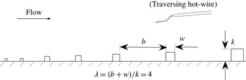
A schematic of the rough wall (
 $k\propto x$
) used in the study of Kameda et al. (Reference Kameda, Mochizuki, Osaka and Higaki2008).

which leads to a contradictory result, i.e.,
 $l\propto x^{1/2}$
. In order to avoid this inconsistency, one has to omit either (2.9g
) or (2.9h
). In other words, one has to drop either
 $(\partial (\overline{u^{\prime 2}}-\overline{v^{\prime 2}}))/\partial x$
or
 ${\it\nu}(\partial ^{2}\bar{U}/\partial y^{2})$
in (2.1b
). When the former term is ignored, we obtain the conditions
 $l\propto x^{1/2}$
and
 $u^{\ast }=(C_{3}/C_{1})U_{1}=$
constant. Note that
 $x^{1/2}$
and
 $U_{1}$
are similar to the scaling parameters in a laminar boundary layer, where viscous effects are dominant. On the other hand, neglecting the viscous term (strictly valid when
 $Re\rightarrow \infty$
), we obtain that
 $l\propto x$
and
 $u^{\ast }=\text{constant}$
. This result is identical to what we would obtain when asymptotic arguments are used when a two-layer model of the boundary layer is considered. In their study, George & Castillo (Reference George and Castillo1997) neglected both
 $(\partial (\overline{u^{\prime 2}}-\overline{v^{\prime 2}}))/\partial x$
and
 ${\it\nu}(\partial ^{2}\bar{U}/\partial y^{2})$
to conclude that
 $U_{1}$
is the velocity scale for the outer region of a turbulent boundary layer. Since they omitted both the conditions (2.9g
) and (2.9h
), they could not obtain a constraint for the length scale. It is important to remember that such assumptions about the individual terms in (2.1b
) can only give solutions to a confined region of the boundary layer (as expected for the two-layer model Townsend Reference Townsend1956) and cannot be valid across the entire boundary layer. Later, Jones et al. (Reference Jones, Nickels and Marusic2008) pointed out that the assumptions made by George & Castillo (Reference George and Castillo1997) prevented them from realising that certain other velocity scales, such as
 $U_{{\it\tau}}$
, are possible. Note that, Jones et al. (Reference Jones, Nickels and Marusic2008) also used asymptotic arguments to show that
 $U_{{\it\tau}}$
is an equally valid velocity scale for the outer region of the boundary layer. This is not consistent with the present SP analysis.
Since neither
 $l\propto x$
nor
 $l\propto x^{1/2}$
are observed in a ZPG smooth-wall turbulent boundary layer, one is forced to conclude that complete SP cannot be achieved in such a flow, as noted by Townsend (Reference Townsend1956) (see also Townsend Reference Townsend1976).
2.2. Rough wall
Let us now consider the case of a turbulent boundary layer where the viscous term in (2.1b
) can be dropped. This would correspond to the case where it is negligible everywhere in the boundary layer. This is likely to be observed on a rough wall made of transverse bars (Leonardi et al.
Reference Leonardi, Orlandi, Smalley, Djenidi and Antonia2003; Kamruzzaman et al.
Reference Kamruzzaman, Djenidi, Antonia and Talluru2015). Leonardi et al. (Reference Leonardi, Orlandi, Smalley, Djenidi and Antonia2003) showed that, relative to a smooth surface, the local viscous friction increases on the roughness top plane and becomes smaller between the roughness elements. They further showed that, when integrated over a wavelength
 ${\it\lambda}$
(see figure 1), the friction force is zero, even slightly negative, when
 $4\leqslant {\it\lambda}/k\leqslant 12$
(see figure 5 in Leonardi et al.
Reference Leonardi, Orlandi, Smalley, Djenidi and Antonia2003); the minimum of the viscous friction and the maximum of the form drag occur when
 ${\it\lambda}/k=8$
. This result has been further corroborated for a turbulent boundary layer by the DNS study of Lee & Sung (Reference Lee and Sung2007). Experimentally, Kamruzzaman et al. (Reference Kamruzzaman, Djenidi, Antonia and Talluru2015) showed that the pressure drag contributed almost totally to the total drag on a rod-roughened wall with
 ${\it\lambda}/k=8$
.
Removing the viscous term from (2.8) amounts to dropping (2.9h
), while all other conditions remain valid. Again we obtain
 $u^{\ast }=(C_{3}/C_{1})U_{1}=$
constant and
 $l\propto x$
. Kameda et al. (Reference Kameda, Mochizuki, Osaka and Higaki2008) showed that, after some initial development length,
 $U_{{\it\tau}}$
becomes a constant over a rough wall where
 $k$
varies linearly with
 $x$
. This implies that
 $U_{{\it\tau}}$
can be identified with
 $u^{\ast }$
in such a rough-wall flow. In this case,
 $U_{{\it\tau}}$
is primarily contributed by the form drag and has practically no contribution from the viscous drag. Using these two conditions (
 $l\propto x$
and
 $u^{\ast }=\text{constant}$
) in (2.9d
), we also find that
 $u^{\ast }/v^{\ast }=\text{constant}$
. Interestingly, it follows from these SP solutions that any of the conditions (2.9i
)–(2.9k
) imposes a constraint that
 $l/k$
must be constant. In other words, both
 $l$
and
 $k$
must vary in
 $x$
in a similar fashion. Since we found that
 $l\propto x$
, this condition implies that
 $k\propto x$
. This condition is similar to Rotta’s (Reference Rotta1962) result,
‘Complete similarity of the turbulent boundary layer on a flat plate can be reconciled with the flow equations if the plate is covered with a roughness distribution continuously varying in such a manner that the representative length scale
 $k_{r}$
of the roughness is everywhere in constant ratio of the distance
 $x$
from the leading edge’. (Taken from Rotta Reference Rotta1962).
However, since Rotta did not consider the form drag term in the mean momentum equation in his analysis, he had to rely on empirical arguments and the law-of-the-wall to arrive at this result. He introduced the roughness height
 $k$
via dimensional analysis in the expression of the velocity, i.e.
 $U_{1}-\langle \bar{U}\rangle =u^{\ast }f(yU_{{\it\tau}}/{\it\nu},kU_{{\it\tau}}/{\it\nu})$
. Such an empirical approach is not required in our analysis as shown above. Therefore, the complete SP solutions obtained in our study are valid across the entire boundary layer thickness.
It is worth mentioning the previous study of Smalley, Antonia & Djenidi (Reference Smalley, Antonia and Djenidi2001), who also obtained SP conditions for a rough-wall turbulent boundary layer. They identified the negligible contribution of the viscous term and removed the term from the analysis. However, since their equation of motion was not space-averaged as it is done here, Smalley et al. (Reference Smalley, Antonia and Djenidi2001) did not have the form drag associated with roughness and hence they could not obtain the SP condition for the roughness height
 $k$
.
The above result indicates that complete SP in a ZPG turbulent boundary layer can be satisfied once the viscous term is negligible or zero everywhere across the boundary layer. This can be achieved on a rough wall made of transverse bars whose height increases proportionally with
 $x$
. It is possible that other types of roughness including 3-D roughness geometries can also lead to complete SP as long as they meet the dynamical and geometrical conditions conform with SP, i.e. negligible viscous force and a roughness height increasing linearly with
 $x$
. Also, one cannot exclude other surface conditions, such as slip conditions, that may lead to complete SP solutions.
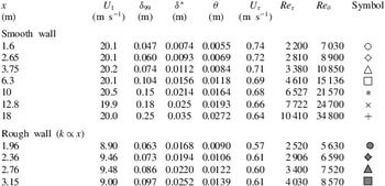
Experimental conditions for the smooth-wall data (Kulandaivelu Reference Kulandaivelu2012) and the rough-wall data (
 $k\propto x$
, Kameda et al. (Reference Kameda, Mochizuki, Osaka and Higaki2008)).

3. Testing SP using experimental results
The above SP conditions are tested in this section using experimental data taken on a smooth wall (Kulandaivelu Reference Kulandaivelu2012) and the rough-wall data (
 $k\propto x$
) of Kameda et al. (Reference Kameda, Mochizuki, Osaka and Higaki2008). A schematic of the roughness used by Kameda et al. (Reference Kameda, Mochizuki, Osaka and Higaki2008) is shown in figure 1. In both these experiments, hot-wire anemometry is used to measure the velocity fluctuations. Full details of these experiments and hot-wire specifications are given in the above cited papers. The experimental conditions of the smooth and rough-wall boundary layers and their respective symbols are listed in table 1. Note that
 ${\it\delta}_{99}$
is used for
 ${\it\delta}$
in both the smooth and rough-wall boundary layers. For the smooth-wall measurements,
 $U_{{\it\tau}}$
has been determined by matching the logarithmic mean velocity profile to the constants
 ${\it\kappa}=0.384$
and
 $A=4.17$
(Chauhan, Nagib & Monkewitz Reference Chauhan, Nagib and Monkewitz2009). For the measurements of Kameda et al. (Reference Kameda, Mochizuki, Osaka and Higaki2008),
 $U_{{\it\tau}}$
has been measured independently using the floating element technique. It is important to note that the profiles in the rough-wall study of Kameda et al. (Reference Kameda, Mochizuki, Osaka and Higaki2008) are only time averaged (Kameda et al. (Reference Kameda, Mochizuki, Osaka and Higaki2008) did not provide space averaged quantities). However, they are taken directly above the roughness elements. One expects that if SP is satisfied then the profiles at consecutive positions
 $x_{{\it\lambda}}/k$
(
 $x_{{\it\lambda}}$
is measured relative to the trailing edge of a roughness element) should collapse when scaled with the SP parameters. Another point to note when dealing with rough wall is the proper identification of the origin for the distance to the wall
 $y$
. This origin is critical when one seeks to validate any law of the wall. However, since the SP analysis is not concerned with the law of the wall, the actual location of the origin is not relevant because it does not affect the SP solutions. We simply used the data of Kameda et al. (Reference Kameda, Mochizuki, Osaka and Higaki2008) where the origin of
 $y$
is taken at the plane located 0.54
 $k$
below the local crest of the roughness elements. Kameda et al. (Reference Kameda, Mochizuki, Osaka and Higaki2008) evaluated this location by following the procedure outlined by Jackson (Reference Jackson1981) and tested in the recent study of Leonardi et al. (Reference Leonardi, Orlandi, Smalley, Djenidi and Antonia2003).
Table 1 shows that
 $U_{{\it\tau}}$
decreases continuously with increasing
 $x$
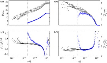
on the smooth wall but is essentially constant over the rough wall, which suggests that SP is achieved over this latter surface. This is further confirmed in figure 2(a–d), where we compare the profiles of the mean velocity, turbulence intensity, skewness and flatness factor of
 $u$
between the smooth and rough-wall flows using
 $U_{{\it\tau}}$
and
 ${\it\delta}$
as scaling parameters (the vertical dashed line in the figures represents the top plane of the roughness elements).
Comparison of profiles of (a) mean velocity; (b) turbulence intensity; (c) skewness and (d) flatness factor of
 $u$
between a smooth wall (Kulandaivelu Reference Kulandaivelu2012) and a rough wall (
 $k\propto x$
, Kameda et al.
Reference Kameda, Mochizuki, Osaka and Higaki2008). The dashed line corresponds to the constant value of
 $k/{\it\delta}$
for the roughness. See table 1 for the grey colored symbols.

Figure 2(a) shows a better collapse of the mean velocity profiles on the rough wall than on the smooth wall, supporting the results from our SP analysis. In particular, the collapse of the rough-wall velocity profiles across the entire boundary layer is consistent with the SP condition (i.e.
 $k\propto x$
) derived above for a rough wall. This is further corroborated by the collapse of second, third and fourth-order moments of the velocity fluctuations over the rough wall. It is easy to see that all the higher-order velocity moments presented in figure 2 have distinctively different distributions compared to the smooth wall. This is because the rough wall has modified the near-wall region of the turbulent boundary layer. The roughness acts in a manner that the viscous mean stress, in particular the friction drag is suppressed, or at least significantly reduced, and the no-slip condition removed. In effect, the roughness has removed the viscous inner layer. In this case, it is not surprising to observe that the rough-wall turbulent boundary layer is in a SP state, since the condition, identified by Townsend (Reference Townsend1956), is met; no viscous inner layer can be part of the complete SP region. Interestingly, this observation shows that not only the two-layer model is no longer applicable on this rough surface, but confirms Townsend (Reference Townsend1956)’s statement that the two-layer model is not compatible with complete SP. Further, the removal of the viscous inner layer by the roughness explains why SP is achievable irrespective of the value of
 $Re$
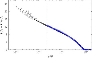
. The removal of the viscous inner layer by the rough wall is well illustrated by plotting the mean velocity defect plots as shown in figure 3. While the smooth wall profiles deviate from each other as the wall is approached, the rough-wall profiles collapse across the entire layer, right down to the plane of the roughness elements.
Comparison of velocity defect profiles in smooth and rough-wall turbulent boundary layers. See table 1 for symbols.

A remark needs to be made regarding the collapse of the smooth-wall profiles as the distance to the wall increases, as observed in figure 3. This would suggest that
 $U_{{\it\tau}}$
and
 ${\it\delta}$
are the scaling parameters across all turbulent boundary layers over both the smooth and rough walls. However, the collapse must be interpreted with caution. To illustrate this, we consider the quantity
 $U_{1}/U_{{\it\tau}}=\sqrt{2/C_{f}}=S$
, which is the ratio of outer and inner velocity scales, namely,
 $U_{1}$
and
 $U_{{\it\tau}}$
, respectively, in a two-layer model. Using (2.10) with
 $u^{\ast }=U_{{\it\tau}}$
, we find that
 $S$
is a constant in a self-preserving rough-wall turbulent boundary layer and its deviation from a constant value indicates a departure from SP. In similar fashion, if
 $U_{{\it\tau}}$
was a SP scaling velocity, the variation of
 $U/U_{{\it\tau}}$
along
 $x$
signifies a departure from SP. This implies that both
 $S$
and
 $U/U_{{\it\tau}}$
are varying in
 $x$
in almost a similar fashion. This is evident in figure 2(a), where the smooth-wall mean velocity profiles at different
 $x$
exhibit a systematic upward shift with increasing
 $x$
across most of the boundary layer. So, when we compute
 $(U_{1}-U)/U_{{\it\tau}}=S-U/U_{{\it\tau}}$
along
 $x$
, we are indeed removing the variation in
 $x$
and therefore, the profiles collapse well. Further, the area under the curve
 $(U_{1}-U)/U_{{\it\tau}}$
versus
 $y/{\it\delta}$
is forced to be unity. Both these constraints impose a bias on the velocity defect plots towards similarity.
4. Conclusions
A SP analysis of a ZPG turbulent boundary layer over rough walls has been carried out with a view to establish the requirements of complete SP (i.e. SP across the entire layer) and assess whether they can be achieved or not. The time and space averaged equation of the streamwise momentum was considered, where the form drag arising from the roughness elements is included.
The results confirm that it is not possible to obtain complete SP in the case of a smooth-wall turbulent boundary layer, except when
 $Re\rightarrow \infty$
. Further, our analysis shows that complete SP is possible over certain rough walls. In this case, the SP analysis leads to the following constraints
 $u^{\ast }=\text{constant}$
,
 $l\propto x$
and
 $k/l=\text{constant}$
, for the velocity and length scales and the roughness height, respectively. These SP conditions are exactly satisfied when the roughness height increases linearly with
 $x$
; this result should apply to both 2-D and 3-D rough surfaces. Although this result conforms to Rotta (Reference Rotta1962)’s condition, it has been obtained more rigorously than by Rotta.
The SP solutions have been tested against experimental data for a ZPG turbulent boundary layer over smooth and rough walls. Compliance with SP is observed for the data of Kameda et al. (Reference Kameda, Mochizuki, Osaka and Higaki2008) over a 2-D rough wall with
 $k\sim x$
but not for the smooth-wall data. Some important observations can be drawn from the present results relating to the statements made by Townsend (Reference Townsend1956) regarding SP of a turbulent boundary layer:
-
(1) Complete SP can be achieved only when the viscous mean stress is zero, or at least negligible (across the entire boundary layer). This appears to be relatively well achieved in a rough wall with a linearly increasing roughness element height. The roughness elements act on the boundary layer in such a manner that the viscous mean stress is zero, or at least negligible in comparison to the form drag.
-
(2) The concept of a two-layer model no longer applies to rough walls which complies with complete SP since the viscous inner layer is effectively removed.
These observations suggest that turbulent boundary layers develop differently over different surface conditions. Caution must therefore be exercised when comparing turbulent boundary layers over smooth walls with boundary layers over rough walls or over different surface conditions (e.g. wall suction/blowing).
Acknowledgements
The authors acknowledge the Australian Research Council for its financial support. We thank Dr T. Kameda at Kinki University for providing his data. We also thank Dr V. Kulandaivelu for providing some of his data taken during his PhD at Melbourne University.