2.1 Base flow and perturbation equations

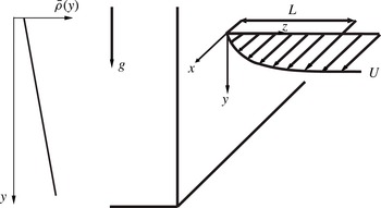
We consider a horizontally directed flow adjacent to a vertical wall in a non-rotating, incompressible viscous stably stratified fluid, as sketched in figure 1. The stratification is assumed to be uniform with a constant buoyancy frequency

where $g$ is gravity, ${\it\rho}_{0}$ is a characteristic value of the mean density $\overline{{\it\rho}}$ . As commonly done in the context of boundary layer stability, we apply a local parallel-flow assumption and assume that the base flow velocity field is given by the tanh profile

where $\boldsymbol{e}_{\boldsymbol{x}}$ is the unit vector in the streamwise direction $x$ . The local characteristic velocity $U$ and boundary layer thickness $L$ are used to non-dimensionalize all the variables. The local parallel-flow assumption gives a constraint on the streamwise perturbation wavelength which should be much smaller than the viscous evolution length. We shall discuss this constraint in § 4.

Figure 1.

Sketch of the flow geometry.

The choice of a tanh profile (instead of a Blasius profile) has been made for numerical convenience. Both the viscous and the radiative instabilities that we discuss here are expected to be weakly sensitive to the details of the profile (as long as it remains non-inflectional). In the very large Reynolds number limit, it is indeed known that the characteristics of these instabilities only depend on the velocity derivatives at the boundary (see Drazin & Reid (Reference Drazin and Reid1981) for the viscous instability and Candelier et al. (Reference Candelier, Le Dizès and Millet2012) for the radiative instability).

The base flow is defined by three parameters:

where ${\it\nu}$ and $D$ are the kinematic viscosity and the mass diffusivity of the fluid.

In the present study, the Froude and Reynolds numbers are varied in the intervals

We neglect the diffusion of mass and set $Sc=\infty$ . This hypothesis is valid for salty water, for which $Sc$ is around 700.

The goal of the present study is to perform a linear temporal stability analysis of the base flow (2.2). Perturbations are then searched in the form of normal modes

where $k_{x}$ and $k_{y}$ are real wavenumbers and ${\it\omega}$ the complex eigenfrequency. The velocity, pressure and buoyancy amplitudes $(u,v,w,p,b)$ satisfy the following equations obtained by linearizing the Navier–Stokes and density equations under the Boussinesq approximation

where

The no-slip boundary condition gives $u(0)=v(0)=w(0)=0$ . Far away from the boundary, we apply a condition of radiation which prescribes that the energy should propagate outward.

2.2 Numerical method

The system (2.6a–e ) is discretized using a pseudo-spectral method on the collocation points of Laguerre polynomials. These polynomials are well adapted to semi-infinite domain $[0,+\infty [\,$ . This method has already been used in Riedinger et al. (Reference Riedinger, Le Dizès and Meunier2010) and Candelier et al. (Reference Candelier, Le Dizès and Millet2012). The system of equations is then transformed into a generalized eigenvalue problem $\boldsymbol{A}\boldsymbol{f}={\it\omega}\boldsymbol{B}\boldsymbol{f}$ for $\boldsymbol{f}=[u,v,w,p,b]$ , which is solved using subroutines of Matlab©.

The eigenfunctions obtained by this method automatically vanish at infinity. As already explained by Riedinger et al. (Reference Riedinger, Le Dizès and Meunier2010), this is not an adequate behaviour for all the physical perturbations.

By considering (2.6) for large $z$ , it is easy to show that all solutions are a sum of exponentials $\text{e}^{\text{i}{\it\beta}z}$ with ${\it\Lambda}=k_{x}^{2}+k_{y}^{2}+{\it\beta}^{2}$ satisfying

The condition of radiation prescribes that the solution should expend at infinity on three exponentials among the six possible (only the exponentials corresponding to waves propagating energy outward are kept). When $\text{Im}({\it\omega})>0$ , this condition of radiation is equivalent to discarding the growing exponentials and keeping the decreasing exponentials. It is therefore equivalent to the vanishing of the solution at infinity. This implies that all unstable modes can a priori be captured by the spectral code. When $\text{Im}({\it\omega})=0$ or $\text{Im}({\it\omega})<0$ , the conditions of radiation and of vanishing do not necessarily match. There are large regions of the complex ${\it\omega}$ plane where these two conditions are not equivalent. In these regions, the modes obtained by the spectral code are therefore ‘unphysical’. 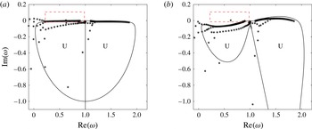The boundaries of these regions correspond to curves in the ${\it\omega}$ plane where one of the wavenumbers ${\it\beta}$ satisfying (2.8) becomes real. These curves are the so-called continuous spectrum. An illustration showing the numerical spectrum and the continuous spectrum is displayed in figure 2(a) for a typical example. In this figure, we have indicated by a dashed rectangle the region of the ${\it\omega}$ plane where the interesting eigenvalues corresponding to the radiative instability are expected. This region is very close to the continuous spectrum, which means that the eigenfunctions decay slowly at infinity. As explained in Riedinger et al. (Reference Riedinger, Le Dizès and Meunier2010), the exponentially decreasing behaviour of the solution can be improved by introducing a complex mapping $z=z^{\prime }\text{e}^{\text{i}{\it\alpha}}$ where ${\it\alpha}$ is a fixed positive angle. Such a mapping modifies an oscillating behaviour on the $z$ variable, say $\text{e}^{\text{i}{\it\beta}z}$ with ${\it\beta}>0$ to an exponentially decreasing behaviour $\text{e}^{\text{i}{\it\beta}\cos {\it\alpha}z^{\prime }}\text{e}^{-{\it\beta}\sin {\it\alpha}z^{\prime }}$ on the $z^{\prime }$ variable. The mapping thus modifies the spectrum and the continuous spectrum as shown in figure 2(b). The unstable mode in the dashed rectangle is now further away from the continuous spectrum curve. Being localized nearer to the origin, this mode is more easily resolved by the pseudo-spectral code. Neutral eigenvalues as well as weakly damped eigenvalues can also be captured by this method.

Figure 2.

Continuous spectrum (solid lines) and numerical eigenvalues (stars) for $N=100$ and the parameters $Re=10^{4}$ , $F=1$ , $k_{x}=1$ , $k_{y}=10$ . The ‘unphysical’ domain is indicated by the letter ‘U’. (a) Integration on the real axis ( ${\it\alpha}=0$ ); (b) integration on a complex path $z^{\prime }=z\text{e}^{-\text{i}{\it\alpha}}$ with ${\it\alpha}={\rm\pi}/20$ . The eigenvalue domain of interest is indicated by the dashed rectangle.

As soon as an eigenvalue is obtained, its robustness is tested by varying the angle ${\it\alpha}$ and the number $N$ of polynomials. We have typically used ${\it\alpha}={\rm\pi}/20$ and $N=100$ .

3.1 Boundary layer instability (Tollmien–Schlichting waves)

Considering a boundary layer flow, the viscous instability associated with TS waves is expected to be active. Without stratification ( $F=\infty$ ), the viscous instability of a boundary layer profile has been known for a long time (see for instance Betchov & Criminale Reference Betchov and Criminale1967). In that case, Squire’s theorem is applicable: the most unstable mode among all the possible wavenumbers $k_{x}$ and $k_{y}$ is obtained for $k_{y}=0$ . Being 2-D without variation in the stratification direction $y$ , this mode is also expected to exist in the presence of stratification, as the equations for the transverse velocity $v$ and the buoyancy $b$ are decoupled from the other velocity components and the pressure. However, there is no Squire theorem which guarantees that this 2-D mode remains the most unstable in the presence of stratification.

Figure 3.

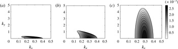
Growth rate contours of the viscous instability in the $(k_{x},k_{y})$ plane for $Re=10^{4}$ and different Froude numbers. (a) $F=\infty$ (unstratified case); (b) $F=1$ ; (c) $F=0.1$ . Contours are every 0.00025 from 0 to 0.0028.

Figure 4.

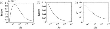
Characteristics of the most unstable TS wave as a function of $Re$ . (a) Growth rate $\text{Im}({\it\omega})$ ; (b) oscillation frequency $\text{Re}({\it\omega})$ ; (c) wavenumber $k_{x}$ .

The effect of the Froude number on the growth rate curve in the $(k_{x},k_{y})$ plane is illustrated in figure 3. In these plots, we do see that for a given Reynolds number, the instability domain associated with the viscous instability grows as the stratification increases while the largest growth rate in this $(k_{x},k_{y})$ domain is still reached for $k_{y}=0$ . We have tried other values of the Reynolds number, and have always found that the most unstable TS wave, among all the possible wavenumbers $k_{x}$ and $k_{y}$ , remains 2-D whatever the Froude number. Since this mode does not depend on $F$ , it means that its characteristics are not affected by the stratification. The characteristics of the most unstable TS wave are therefore independent of the stratification. They are shown in figure 4 as a function of the Reynolds number. The critical Reynolds number is found to be $Re_{c}^{(v)}\approx 3981$ for which the critical TS wave has the characteristics: $k_{x}=0.35$ , ${\it\omega}=0.1$ . The growth rate decreases for large Reynolds numbers. It reaches its maximum at the most dangerous Reynolds number $Re_{m}^{(v)}\approx 22\,390$ for the most dangerous mode of characteristics $k_{x}=0.13$ , ${\it\omega}=0.016+0.0033\text{i}$ .

Figure 5.

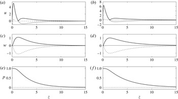
Eigenfunctions of the most unstable TS wave ((a,b) streamwise velocity $u$ ; (c,d) normal velocity $w$ ; (e,f) pressure $p$ ) for the critical Reynolds number $Re=Re_{c}^{(v)}\approx 3981$ (a,c,e) and the most dangerous Reynolds number $Re=Re_{m}^{(v)}\approx 22\,390$ (b,d,f). Thick solid lines, solid lines and dashed lines represent absolute value, real part and imaginary part, respectively.

The eigenfunctions of the critical and most dangerous TS waves are presented in figure 5. Note that the eigenfunctions of both modes are very similar. The only noticeable difference is the stronger localization of the critical mode close to the boundary. This can be related to the streamwise wavenumber difference and the behaviour in $\text{e}^{-k_{x}z}$ of the eigenfunctions far from the boundary.

Figure 6.

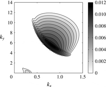
Growth rate contours in the $(k_{x},k_{y})$ plane for $Re=10^{4}$ and $F=1$ (enlarged view of figure 3 b). The two regions correspond to the viscous and radiative instability respectively. Contours are every 0.001 from 0.001 to 0.012.

The evidence that Squire’s theorem is not applicable in the presence of stratification is given in figure 6 which is an extension in a larger $(k_{x},k_{y})$ domain of the growth rate contours. We clearly see the presence of 3-D modes which are more unstable than all the 2-D modes. These 3-D unstable modes are associated with another instability, the so-called radiative instability, analysed in the next section.

3.2 Radiative instability

The radiative instability is inviscid in nature and results from the coupling between shear and internal gravity waves associated with the fluid stratification. The inviscid characteristics of this instability have been obtained for the tanh boundary layer profile in Candelier et al. (Reference Candelier, Le Dizès and Millet2012).

Figure 7.

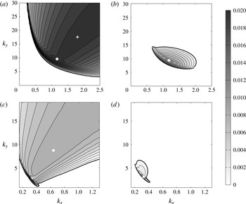
Growth rate contours of the radiative mode in the $(k_{x},k_{y})$ plane for several sets of Froude and Reynolds numbers. (a) $Re=10^{7}$ , $F=0.5$ ; (b) $Re=10^{4}$ , $F=0.5$ ; (c)  $Re=10^{7}$ , $F=3$ ; (d) $Re=10^{4}$ , $F=3$ . White crosses indicate local maxima of the growth rate, the largest maximum being shown with an asterix. Contours are every 0.001 from 0.001 to 0.02.

In figure 7, we have plotted the growth rate of the (most unstable) radiative mode in the $(k_{x},k_{y})$ plane for various Froude and Reynolds numbers. (Several unstable radiative modes may exist for a given set of parameters $(k_{x},k_{y},Re,F)$ . We always keep the mode with the largest growth rate even if we do not systematically mention that it is the most unstable radiative mode). We clearly see that viscous effects reduce the domain of instability. In the inviscid limit, the maximum growth rate is obtained for infinite $k_{x}$ and $k_{y}$ (Candelier et al. Reference Candelier, Le Dizès and Millet2012). As soon as viscous effects are present, the maximum growth rate is reached for finite $k_{x}$ and finite $k_{y}$ . 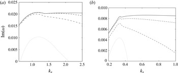In figure 8, we have plotted the maximal value of the growth rate over all $k_{y}$ as a function of $k_{x}$ for various Reynolds numbers and $F=0.5$ and $3$ . The viscous damping of higher wavenumbers is also clearly seen on these plots. It should be noticed that there are the two local peaks of the growth rate curve for $Re=10^{6}$ and $10^{7}$ . These peaks have also been indicated by symbols in figure 7(a,c). While the first peak remains almost fixed, the location of the second peak strongly varies with Reynolds number. This strong variation can be associated with the extremely broad character of this peak and the fact that it goes to infinity as $Re\rightarrow \infty$ .

Figure 8.

Maximum growth rate $\max _{k_{y}}[\text{Im}({\it\omega})]$ of the radiative modes versus $k_{x}$ for $F=0.5$ (a) and $F=3$ (b). Solid line: $Re=10^{7}$ , dashed line: $Re=10^{6}$ , dash-dot line: $Re=10^{5}$ , dotted line: $Re=10^{4}$ .

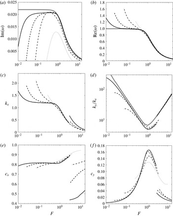
In figure 9, we have plotted the characteristics of the most unstable radiative mode (growth rate maximized over all the possible wavenumbers $(k_{x},k_{y})$ ) as a function of the Froude number for different Reynolds numbers. As expected, viscous results tend to inviscid results as $Re$ increases. Note however that the convergence is slow, especially for small Froude numbers. This can be explained by the fact that even for $Re=10^{7}$ , the most unstable wavenumbers are still of order 1 (remember, they should go to infinity in the inviscid limit). For this Reynolds number, the most unstable wavenumbers correspond to the first peak of the growth rate curve in the $(k_{x},k_{y})$ plane for all Froude numbers $F<1$ (see figure 7 a). It jumps to the second local peak of larger wavenumbers for higher Reynolds numbers, or for larger Froude numbers (see figure 7 c). This change of modes as Froude or Reynolds number increases generates the jump observed in figure 9(c–f).

Figure 9.

Characteristics of the most unstable radiative mode (obtained by maximizing the growth rate over all $k_{x}$ and $k_{y}$ ) as a function of the Froude number $F$ for different Reynolds numbers. $Re=10^{4}$ (dotted line), $10^{5}$ (dash-dot line), $10^{6}$ (dashed line), $10^{7}$ (solid line), $\infty$ (thick grey line). (a) Growth rate $\text{Im}({\it\omega})$ ; (b) oscillation frequency $\text{Re}({\it\omega})$ ; (c) streamwise wavenumber $k_{x}$ ; (d) wavenumber ratio $k_{y}/k_{x}$ ; (e) phase velocity $\text{Re}({\it\omega})/k_{x}$ along $x$ ; (f) phase velocity $\text{Re}({\it\omega})/k_{y}$ along $y$ .

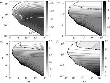
The results for the radiative instability are summarized in figure 10. In this figure, we have displayed the characteristics of the most unstable radiative mode as a function of both parameters $Re$ and $F$ . Only the growth rate contours are expected to be smoothed. The frequency, wavenumbers and phase velocities exhibit discontinuities which are associated with the local growth rate peak jumps discussed above. We have observed a single jump which is indicated by the dashed line in figure 10(b–d).

The critical Reynolds number for the radiative instability is found to be $Re_{c}^{(r)}\approx 1995$ and is reached for $F_{c}^{(r)}\approx 1.51$ . The characteristics of the critical radiative mode are $k_{x}\approx 0.615$ , $k_{y}\approx 4.236$ , ${\it\omega}\approx 0.535$ . As expected, the Froude number instability range increases with the Reynolds number, but the most unstable growth rates are obtained for strongly stratified configurations for which $F$ is smaller than 1. In figure 10(a), the white dotted line gives the Froude number which maximizes the radiative instability for a prescribed Reynolds number.

Figure 10.

Characteristics of the most unstable radiative mode (obtained by maximizing the growth rate over all $k_{x}$ and $k_{y}$ ) in the $(Re,F)$ plane. (a) Growth rate $(\text{Im}({\it\omega}))$ contours; (b) oscillation frequency $(\text{Re}({\it\omega}))$ contours (in the unstable region); (c) streamwise wavenumber ( $k_{x}$ ) contours; (d) transverse wavenumber ( $k_{y}$ ) contours. The black dashed line indicates a discontinuity. The white dotted line in (a) gives the value of $F$ which maximizes the growth rate for a fixed $Re$ .

The behaviour of constant growth rate curves for small Froude and large Reynolds numbers can be obtained by adding the viscous corrections to the non-viscous estimate. In this limit, Candelier et al. (Reference Candelier, Le Dizès and Millet2012) have indeed shown that the most unstable inviscid mode was obtained for $k_{y}/k_{x}\sim 4.9/F$ . This means that for small $F$ , $k_{y}$ is much larger than $k_{x}$ as well as the wavenumber based on the characteristic scale in the normal direction ( $z$ ) which varies as $k_{x}$ . The viscous damping of the mode is then expected to be just $-k_{y}^{2}/Re$ . If we assume that $k_{x}$ is approximately constant, this gives a viscous growth rate which is constant on the line $Re\,F^{2}=\text{Cst}$ , as approximately observed in figure 10(a).

Figure 11.

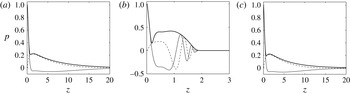
Pressure eigenfunction of distinguished radiative modes for $F=3$ and two Reynolds numbers (corresponding to the symbols of figure 7 c,d). (a) Most unstable mode for $Re=10^{4}$ : $k_{x}=0.33$ , $k_{y}=3.13$ , ${\it\omega}=0.2971+0.0043\text{i}$ ; (b) most unstable mode for $Re=10^{7}$ : $k_{x}=0.64$ , $k_{y}=8.75$ , ${\it\omega}=0.2817+0.0086\text{i}$ ; (c) less unstable mode corresponding to the first local peak of the growth rate curves for $Re=10^{7}$ : $k_{x}=0.34$ , $k_{y}=2.75$ , ${\it\omega}=0.3023+0.0084\text{i}$ . Thick solid lines, solid lines and dashed lines represent absolute value, real part and imaginary part, respectively.

The eigenfunctions of the distinguished radiative modes marked by symbols in figure 7 are shown in figures 11 and 12. Figure 11(a,b) shows the pressure eigenfunction of the most unstable mode for a weakly stratified configuration ( $F=3$ ) at $Re=10^{4}$ and $10^{7}$ . The pressure eigenfunction for $Re=10^{7}$ strongly resembles the inviscid eigenfunction obtained by Candelier et al. (Reference Candelier, Le Dizès and Millet2012) for large Froude numbers and large wavenumbers. For smaller Reynolds numbers, the eigenfunction is by contrast different. These differences are not due to a change of instability mode. The modes are on the same instability branch but they are associated with two different local peaks of the growth rate contours in the $(k_{x},k_{y})$ plane. For $Re=10^{4}$ , the most unstable mode corresponds to the first peak, while it is the second peak for $Re=10^{7}$ (see figure 7 c). It should be noted that the mode associated with the first peak is still unstable for $Re=10^{7}$ , and its pressure eigenfunction is the same as for $Re=10^{4}$ , as seen in figure 11(c).

Figure 12.

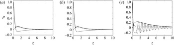
Pressure eigenfunction of distinguished radiative modes for $F=0.5$ and two Reynolds numbers (corresponding to the symbols of figure 7 a,b). (a) Most unstable mode for $Re=10^{4}$ : $k_{x}=1.18$ , $k_{y}=9.34$ , ${\it\omega}=0.964+0.011\text{i}$ ; (b) most unstable mode for $Re=10^{7}$ : $k_{x}=1.17$ , $k_{y}=9.58$ , ${\it\omega}=0.9499+0.0209\text{i}$ ; (c) slightly less unstable mode for $Re=10^{7}$ corresponding to the second local peak of the growth rate curves: $k_{x}=1.80$ , $k_{y}=17.56$ , ${\it\omega}=0.928+0.0209\text{i}$ . Thick solid lines, solid lines and dashed lines represent absolute value, real part and imaginary part, respectively.

In figure 12, we have considered a strongly stratified case ( $F=0.5$ ). Figure 12(a,b) shows the pressure eigenfunction of the most unstable radiative mode for two different Reynolds numbers. By comparing these two figures, we observe that the impact of the Reynolds number is much weaker than for the weakly stratified case, as the pressure eigenfunction is almost not modified. Besides, this eigenfunction is very similar to the eigenfunction of the most unstable mode obtained for $Re=10^{4}$ and $F=3$ . However, it is very different from the most unstable inviscid eigenfunction obtained by Candelier et al. (Reference Candelier, Le Dizès and Millet2012) for small Froude numbers. The inviscid mode exhibits an oscillating structure which is not present in the viscous mode for $Re=10^{4}$ and $Re=10^{7}$ (see figure 12 a,b). This difference is mainly due to a property already mentioned above: the viscous mode is associated with the first peak and has a small streamwise wavenumber (as for the modes shown in figure 11 a,c). We suspect that this peak could be of viscous nature. It indeed gives a mode with a non-oscillating structure which resembles that of 2-D TS waves (see figure 5). If we consider the mode associated with the second peak, we obtain an eigenfunction with an oscillatory tail (figure 12 c) which resembles the inviscid eigenfunction obtained for small Froude numbers (see Candelier et al. (Reference Candelier, Le Dizès and Millet2012, figure 4)). It is important to stress that this mode has almost the same growth rate as the most unstable mode.

Figure 13.

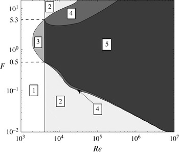
Domains of instability in the $(Re,F)$ plane. (1) No instability; (2) viscous instability without radiative instability; (3) radiative instability without viscous instability; (4) both instabilities present but viscous instability dominates radiative instability; (5) both instabilities present but radiative instability dominates viscous instability.

3.3 Competition between radiative instability and viscous instability

As shown above, the viscous instability is present as soon as $Re>3981$ for any Froude number, while the radiative instability is active in a domain of the $(Re,F)$ plane which has been displayed in figure 10(a). Both instabilities are then expected to be in competition in a large domain of the parameter space. In figure 13, we have provided a summary of this competition by indicating 5 different domains corresponding to a domain of no instability, 2 domains where there is a single instability active, 2 other domains where one instability dominates the other. This figure clearly demonstrates that the radiative instability is the dominant instability in a large domain of the parameter space. It is the first instability to appear as the Reynolds number increases in the range $0.5<F<5.3$ . For $Re=10^{6}$ , it dominates the viscous instability in the large range $0.03<F<30$ .