


1 Introduction
1.1 About the data
The Princeton superpipe (PSP) data measured by Zagarola (Reference Zagarola1996) and described by Zagarola & Smits (Reference Zagarola and Smits1998) comprise 26 velocity profiles that cover three orders of magnitude in the Reynolds number from the moderate value of profile 1,
 $Re=19\,639$
, to the very high value of profile 26,
 $Re=20\,088\,000$
, based on pipe radius (64.68 mm) and pipe centreline velocity. The original Zagarola (Reference Zagarola1996) data were measured using a
 $p_{d}=0.9~\text{mm}$
diameter pitot tube positioned at 52 points across the pipe including 10 points beyond the pipe centreline that were used to check the symmetry of the profiles. The probe diameter limited the position of the centreline of the pitot tube to
 $y=0.9~\text{mm}$
for the first data point above the wall leaving approximately one probe radius of clearance to the wall. This is well outside the viscous wall layer, defined later in this paper as the sublayer
 $(y^{+}<8.3)$
plus the buffer layer
 $(8.3<y^{+}<65)$
, for all but the lowest Reynolds number surveys. Nineteen additional surveys at Reynolds numbers corresponding to the Zagarola (Reference Zagarola1996) experiments were repeated by Jiang, Li & Smits (Reference Jiang, Li and Smits2003) using a
 $p_{d}=0.3~\text{mm}$
diameter pitot tube positioned at 57 points across the pipe including one point beyond the pipe centreline. McKeon (Reference McKeon2003) and McKeon et al. (Reference McKeon, Li, Jiang, Morrison and Smits2003) provide an extensive discussion of methods for correcting the Jiang et al. (Reference Jiang, Li and Smits2003) data as well as tables of corrected and uncorrected velocity data. The
 $p_{d}=0.3~\text{mm}$
pitot tube permits the centreline of the tube to be positioned just
 $y=0.3~\text{mm}$
above the wall for the first data point, again leaving one probe radius of clearance. This allowed valuable data to be taken within and just outside the viscous wall layer over a significant portion of the Reynolds number range of the 19 surveys. In the present paper, the 19 corrected
 $p_{d}=0.3~\text{mm}$
pitot tube surveys are combined with 7 corrected
 $p_{d}=0.9~\text{mm}$
surveys to form a complete set of 26 corrected velocity profiles. The methods used to correct all 26 of the
 $p_{d}=0.9~\text{mm}$
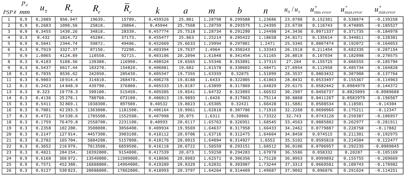
surveys are described in § 4 of this paper and a comparison of the two sets of corrected data is presented in figure 6. Run conditions for the combined set of 26 surveys are provided in table 1. McKeon (Reference McKeon2003) discusses possible roughness effects on the data, particularly at the highest Reynolds numbers. The root-mean-square roughness height of the superpipe surface was measured to be
 $k_{rms}=0.15~\unicode[STIX]{x03BC}\text{m}$
corresponding to
 $k_{rms}/\unicode[STIX]{x1D6FF}=2.32\times 10^{-6}$
. At the highest Reynolds number,
 $R_{\unicode[STIX]{x1D70F}}=530\,023$
, this corresponds to a roughness height Reynolds number of
 $k_{rms}u_{\unicode[STIX]{x1D70F}}/\unicode[STIX]{x1D708}=1.23$
.
1.2 Background
Questions about the high Reynolds number behaviour of wall-bounded flows invariably focus on the structure of the Reynolds stresses and the mean velocity near the wall where viscous effects dominate. Unfortunately, direct measurements of these quantities are often very difficult to make and it may be necessary to infer the near-wall behaviour from measurements away the wall. Fortunately, in a limited region above the wall, virtually all wall-bounded flows tend to approximately follow the law of the wall
 $u/u_{\unicode[STIX]{x1D70F}}=\ln (yu_{\unicode[STIX]{x1D70F}}/\unicode[STIX]{x1D708})/k+C$
where
 $u_{\unicode[STIX]{x1D70F}}=\sqrt{-\unicode[STIX]{x1D70F}_{wall}/\unicode[STIX]{x1D70C}}$
is the friction velocity. The Kármán constant,
 $k$
, and the additive constant,
 $C$
, are experimentally determined quantities. If the constants are known, velocity measurements in the logarithmic region combined with the law of the wall can be used to infer
 $u_{\unicode[STIX]{x1D70F}}$
and therefore the wall shear stress, without having to instrument the wall or directly measure the linear part of the velocity profile.

The law of the wall is the main point of departure for a vast literature directed at questions such as: What friction law covers the widest possible Reynolds number range, (Quarmby Reference Quarmby1969; McKeon et al. Reference McKeon, Li, Jiang, Morrison and Smits2004a ,Reference McKeon, Swanson, Zagarola, Donnelly and Smits b ; McKeon, Zagarola & Smits Reference McKeon, Zagarola and Smits2005; Joseph & Yang Reference Joseph and Yang2010)? Is the Kármán constant really constant and what is its value (Huffman & Bradshaw Reference Huffman and Bradshaw1972)? Would the velocity profile in the intermediate region be better approximated by a power law instead of a logarithm (Barenblatt Reference Barenblatt1993; Barenblatt & Prostokishin Reference Barenblatt and Prostokishin1993; Barenblatt & Chorin Reference Barenblatt and Chorin1996; Barenblatt Reference Barenblatt1999)? How do the mean velocity, Reynolds normal stresses and higher moments of the velocity field scale at low, moderate and high Reynolds numbers (McKeon & Morrison Reference McKeon and Morrison2007; Wu & Moin Reference Wu and Moin2008; Inoue & Pullin Reference Inoue and Pullin2011; Hultmark Reference Hultmark2012; El Khoury et al. Reference El Khoury, Schlatter, Noorani, Fischer, Brethouwer and Johansson2013; Pullin, Inoue & Saito Reference Pullin, Inoue and Saito2013; Ahn et al. Reference Ahn, Lee, Lee, Kang and Sung2015; Morrill-Winter, Phillip & Klewicki Reference Morrill-Winter, Phillip and Klewicki2017)? This is a short list of the many issues around wall flow that remain poorly understood and a complete, relatively recent, summary can be found in Marusic et al. (Reference Marusic, McKeon, Monkewitz, Nagib, Smits and Sreenivasan2010). Much of the effort to answer these questions is directed at finding the best approximation to the data in the viscous wall layer, the intermediate log region and the outer flow wake region and identifying the functions that provide accurate matching between the several layers of the flow (She, Chen & Hussain Reference She, Chen and Hussain2017).
In the present paper, classical mixing length theory is combined with a new wall–wake mixing length function to solve the streamwise momentum equation. The resulting model velocity profile contains five free parameters. An optimization procedure is used to determine the parameter values that produce the minimum squared error for each of the 26 PSP surveys. The resulting model velocity profile is described as ‘universal’ for three reasons (i) it is uniformly valid from the wall to the pipe centreline at all Reynolds numbers, (ii) optimal parameter values vary relatively little across all 26 PSP surveys and (iii) virtually all of the known scalings of the various layers of the flow are captured in the universal profile. In fact, choosing constant values for all five parameters produces a reasonable approximation to the entire set of velocity surveys and associated friction data. Where significant variations in optimal parameter values do occur, they seem to be associated with real physical changes in the flow.
2 Mean flow equations and notation
The mean velocity in pipe flow is governed by the axial balance between the pressure gradient and shear stress.
 $$\begin{eqnarray}\displaystyle \frac{1}{r}\frac{\text{d}}{\text{d}r}(r(\overline{u^{\prime }v^{\prime }}))-\unicode[STIX]{x1D708}\frac{1}{r}\frac{\text{d}}{\text{d}r}\left(r\frac{\text{d}u}{\text{d}r}\right)+\frac{1}{\unicode[STIX]{x1D70C}}\frac{\text{d}p(x,r)}{\text{d}x}=0. & & \displaystyle\end{eqnarray}$$
Throughout this paper, the pipe centreline velocity,
 $u_{0}$
, and radius,
 $\unicode[STIX]{x1D6FF}$
, will be the normalizing velocity and length scales as indicated in figure 1. Thus let
 $$\begin{eqnarray}\displaystyle \left.\begin{array}{@{}c@{}}\displaystyle \unicode[STIX]{x1D702}=\frac{r}{\unicode[STIX]{x1D6FF}}\\ \displaystyle U=\frac{u}{u_{0}}\\ \displaystyle R_{e}=\frac{u_{0}\unicode[STIX]{x1D6FF}}{\unicode[STIX]{x1D708}}\\ \displaystyle \unicode[STIX]{x1D70F}_{w}=\unicode[STIX]{x1D707}\left.\frac{\text{d}u}{\text{d}r}\right|_{r=\unicode[STIX]{x1D6FF}}\\ \displaystyle C_{f}=-\frac{2\unicode[STIX]{x1D70F}_{w}}{\unicode[STIX]{x1D70C}u_{0}^{2}}=2\frac{u_{\unicode[STIX]{x1D70F}}^{2}}{u_{0}^{2}}\\ \displaystyle \frac{1}{\unicode[STIX]{x1D70C}}\frac{\text{d}p(x,r)}{\text{d}x}=\frac{2}{\unicode[STIX]{x1D6FF}}\left(\frac{\unicode[STIX]{x1D70F}_{w}}{\unicode[STIX]{x1D70C}}\right)\\ \displaystyle \unicode[STIX]{x1D70F}=-\frac{\overline{u^{\prime }v^{\prime }}}{{u_{0}}^{2}}.\end{array}\right\} & & \displaystyle\end{eqnarray}$$
Pipe flow sketch and notation.

In dimensionless form, the governing equation (2.1) is
 $$\begin{eqnarray}\displaystyle \frac{\text{d}(\unicode[STIX]{x1D702}\unicode[STIX]{x1D70F})}{\text{d}\unicode[STIX]{x1D702}}+\frac{1}{R_{e}}\frac{\text{d}}{\text{d}\unicode[STIX]{x1D702}}\left(\unicode[STIX]{x1D702}\frac{\text{d}U}{\text{d}\unicode[STIX]{x1D702}}\right)+C_{f}\unicode[STIX]{x1D702}=0. & & \displaystyle\end{eqnarray}$$
If the flow is laminar, the Reynolds shear stress term is zero, the pressure is independent of radius and the velocity profile is
 $$\begin{eqnarray}\displaystyle U(\unicode[STIX]{x1D702})=(1-\unicode[STIX]{x1D702}^{2}). & & \displaystyle\end{eqnarray}$$
The dependence of the laminar skin friction coefficient on pipe Reynolds number is
 $$\begin{eqnarray}\displaystyle C_{f}=\frac{4}{R_{e}}. & & \displaystyle\end{eqnarray}$$
If the flow is turbulent, the dependence of the streamwise pressure gradient on radius is assumed to be negligible. Integrate (2.3) once and apply the centreline boundary condition
 $\text{d}U/\text{d}\unicode[STIX]{x1D702}=\unicode[STIX]{x1D70F}=0$
at
 $\unicode[STIX]{x1D702}=0$
. Equation (2.1) becomes
 $$\begin{eqnarray}\displaystyle \unicode[STIX]{x1D70F}(\unicode[STIX]{x1D702})+\frac{1}{R_{e}}\frac{\text{d}U}{\text{d}\unicode[STIX]{x1D702}}+\frac{C_{f}}{2}\unicode[STIX]{x1D702}=0. & & \displaystyle\end{eqnarray}$$
Note that
 $\unicode[STIX]{x1D70F}<0$
,
 $\text{d}U/\text{d}\unicode[STIX]{x1D702}<0$
and
 $C_{f}>0$
. We are mainly interested in the turbulent case, and so at this point it is convenient to express (2.6) in terms of wall variables.
 $$\begin{eqnarray}\displaystyle \left.\begin{array}{@{}c@{}}\displaystyle u_{\unicode[STIX]{x1D70F}}=\left(-\frac{\unicode[STIX]{x1D70F}_{w}}{\unicode[STIX]{x1D70C}}\right)^{1/2}\\ \displaystyle R_{\unicode[STIX]{x1D70F}}=\frac{\unicode[STIX]{x1D6FF}u_{\unicode[STIX]{x1D70F}}}{\unicode[STIX]{x1D708}}\\ \displaystyle u^{+}=\frac{u}{u_{\unicode[STIX]{x1D70F}}}=\frac{R_{e}}{R_{\unicode[STIX]{x1D70F}}}U\\ \displaystyle y=\unicode[STIX]{x1D6FF}-r\\ \displaystyle y^{+}=\frac{yu_{\unicode[STIX]{x1D70F}}}{\unicode[STIX]{x1D708}}=(1-\unicode[STIX]{x1D702})R_{\unicode[STIX]{x1D70F}}\\ \displaystyle \unicode[STIX]{x1D70F}^{+}=\frac{\overline{u^{\prime }v^{\prime }}}{u_{\unicode[STIX]{x1D70F}}^{2}}=-\left(\frac{R_{e}}{R_{\unicode[STIX]{x1D70F}}}\right)^{2}\unicode[STIX]{x1D70F}.\end{array}\right\} & & \displaystyle\end{eqnarray}$$
The quantity
 $R_{\unicode[STIX]{x1D70F}}=\unicode[STIX]{x1D6FF}u_{\unicode[STIX]{x1D70F}}/\unicode[STIX]{x1D708}$
is often called the Kármán number and symbolized as
 $\unicode[STIX]{x1D6FF}^{+}$
although throughout this paper we will simply call it the friction Reynolds number. The friction velocity, friction coefficient, friction Reynolds number and pipe Reynolds number are all related through the identity
 $$\begin{eqnarray}\displaystyle \frac{u_{0}}{u_{\unicode[STIX]{x1D70F}}}\equiv \frac{R_{e}}{R_{\unicode[STIX]{x1D70F}}}\equiv \sqrt{\frac{2}{C_{f}}}. & & \displaystyle\end{eqnarray}$$
Later on when friction laws are discussed it will generally be in terms of
 $u_{0}/u_{\unicode[STIX]{x1D70F}}$
.
Using (2.7), the governing equation (2.6) becomes
 $$\begin{eqnarray}\displaystyle \unicode[STIX]{x1D70F}^{+}+\frac{\text{d}u^{+}}{\text{d}y^{+}}-\left(1-\frac{y^{+}}{R_{\unicode[STIX]{x1D70F}}}\right)=0. & & \displaystyle\end{eqnarray}$$
For later reference, the laminar velocity and wall friction, equations (2.4) and (2.5), expressed in terms of wall variables are
 $$\begin{eqnarray}\displaystyle u_{laminar}^{+}=y^{+}\left(1-\frac{y^{+}}{2R_{\unicode[STIX]{x1D70F}}}\right) & & \displaystyle\end{eqnarray}$$
and
 $$\begin{eqnarray}\displaystyle C_{f_{laminar}}=\frac{8}{{R_{\unicode[STIX]{x1D70F}}}^{2}}. & & \displaystyle\end{eqnarray}$$
It should be noted that the mean flow equation that governs plane channel flow is virtually identical to (2.9). It would be straightforward to carry over the model velocity profile and all of the analysis used in this paper to the planar case.
2.1 Why use
 $u_{0}$
as the normalizing velocity?

It should be noted that it is a little unusual to use the centreline velocity,
 $u_{0}$
, as the normalizing velocity scale. More commonly one uses the area averaged, or bulk, velocity
 $$\begin{eqnarray}\displaystyle \bar{u}=\frac{2}{\unicode[STIX]{x1D6FF}^{2}}\int _{0}^{\unicode[STIX]{x1D6FF}}ur\,\text{d}r & & \displaystyle\end{eqnarray}$$
while the pipe resistance is expressed in terms of the friction factor
 $$\begin{eqnarray}\displaystyle f=8\left(\frac{u_{\unicode[STIX]{x1D70F}}}{\bar{u}}\right)^{2}=4\overline{C_{f}}, & & \displaystyle\end{eqnarray}$$
where
 $\overline{C_{f}}$
is the friction coefficient normalized by
 $\bar{u}$
. The most easily accessible information about a pipe flow is the mass flow rate
 ${\dot{m}}=\unicode[STIX]{x1D70C}\bar{u}A$
, which is usually specified, and the pressure gradient which determines the wall friction,
 $\unicode[STIX]{x1D70F}_{w}=(\unicode[STIX]{x1D6FF}/2)\text{d}p_{w}/\text{d}x$
, and so it makes practical sense to use
 $\bar{u}$
to normalize everything. Also, to a surprising degree of accuracy, the law of the wall
 $$\begin{eqnarray}\displaystyle u^{+}=\frac{1}{k}\ln (y^{+})+C & & \displaystyle\end{eqnarray}$$
can be used as an approximation to the flow over the whole pipe. This is despite the singularity in the logarithm at the wall and the finite derivative of the log at the pipe centreline. Using (2.14) the bulk velocity integrates to
 $$\begin{eqnarray}\displaystyle \frac{\bar{u}}{u_{\unicode[STIX]{x1D70F}}}=\frac{2}{R_{\unicode[STIX]{x1D70F}}}\int _{0}^{R_{\unicode[STIX]{x1D70F}}}\left(\frac{1}{k}\ln (y^{+})+C\right)\left(1-\frac{y^{+}}{R_{\unicode[STIX]{x1D70F}}}\right)\text{d}y^{+}=\frac{1}{k}\ln (R_{\unicode[STIX]{x1D70F}})+C-\frac{3}{2k}. & & \displaystyle\end{eqnarray}$$
This simple result provides a very attractive direct connection to the law of the wall.
Data from PSP surveys 1 to 26 for
 $\bar{u}/u_{0}$
are shown in figure 2(a), and friction data,
 $u_{0}/u_{\unicode[STIX]{x1D70F}}$
and
 $\bar{u}/u_{\unicode[STIX]{x1D70F}}$
versus
 $R_{\unicode[STIX]{x1D70F}}$
, are presented in figure 2(b). The solid lines are generated using the functional form of (2.14) and (2.15) with the constants
 $k$
and
 $C$
selected to give least squares log–linear fits to the data. At first one might expect that
 $k_{u_{0}/u_{\unicode[STIX]{x1D70F}}}>k_{\bar{u}/u_{\unicode[STIX]{x1D70F}}}$
, as is the case in figure 2(b), because of the general tendency for
 $\bar{u}/u_{0}$
to increase slowly toward one with increasing Reynolds number. But there is no reason to expect the curves in figure 2(b) to eventually intersect. As long as the difference between the additive constants does not change,
 $\lim _{R_{\unicode[STIX]{x1D70F}}\rightarrow \infty }\bar{u}/u_{0}=1$
. Moreover, according to (2.15) the values of
 $k$
for
 $u_{0}/u_{\unicode[STIX]{x1D70F}}$
and
 $\bar{u}/u_{\unicode[STIX]{x1D70F}}$
versus
 $R_{\unicode[STIX]{x1D70F}}$
should be the same as the
 $k$
that appears in (2.14). Indeed, the empirically determined
 $k$
values in figure 2(b) are very close but the displacement between the curves is considerably more than the
 $3/2k$
that appears in (2.15). Clearly a better approximation to the velocity profile than (2.14) is needed.
(a) PSP survey data for
 $\bar{u}/u_{0}$
and (b) wall shear stress in terms of
 $\bar{u}/u_{\unicode[STIX]{x1D70F}}$
and
 $u_{0}/u_{\unicode[STIX]{x1D70F}}$
versus
 $R_{\unicode[STIX]{x1D70F}}$
. Open circles in (b) (○) are data for PSP surveys 1 to 26. Least square log–linear fits to the data for PSP surveys 6 to 26 are shown as solid lines. Root-mean-square error in the upper solid line is 0.112 in units of
 $u^{+}$
. Root-mean-square error in the lower solid line is 0.0975.

The goal in this paper is to approximate as accurately as possible the PSP velocity profiles, and for this it is necessary to integrate (2.1) where the outer boundary condition is
 $u/u_{0}=1$
for all
 $R_{\unicode[STIX]{x1D70F}}$
. This way the added complexity of the Reynolds number dependence of
 $\bar{u}/u_{0}$
is avoided. In the end we will see that the simple log–linear behaviour of
 $u_{0}/u_{\unicode[STIX]{x1D70F}}$
and
 $\bar{u}/u_{\unicode[STIX]{x1D70F}}$
, which dates back to Prandtl (Reference Prandtl and Durand1934a
), is generated rigorously by the universal model velocity profile derived in the next section.
3 Mixing length model for the turbulent shear stress
We use classical mixing length theory to relate the turbulent shear stress to the mean velocity (Prandtl Reference Prandtl and Durand1934b , Reference Prandtl1949; van Driest Reference van Driest1956; Nikuradse Reference Nikuradse1966).
 $$\begin{eqnarray}\displaystyle \unicode[STIX]{x1D70F}^{+}=\left(\unicode[STIX]{x1D706}(y^{+})\frac{\text{d}u^{+}}{\text{d}y^{+}}\right)^{2}. & & \displaystyle\end{eqnarray}$$
The mixing length function
 $\unicode[STIX]{x1D706}(y^{+})$
is positive, increases monotonically with
 $y^{+}$
, is analytic at
 $y^{+}=0$
and
 $\unicode[STIX]{x1D706}\rightarrow 0$
as
 $y^{+}\rightarrow 0$
. Insert (3.1) into (2.9). The result is a quadratic equation for the velocity derivative.
 $$\begin{eqnarray}\displaystyle \left(\frac{\text{d}u^{+}}{\text{d}y^{+}}\right)^{2}+\frac{1}{\unicode[STIX]{x1D706}(y^{+})^{2}}\frac{\text{d}u^{+}}{\text{d}y^{+}}-\frac{1}{\unicode[STIX]{x1D706}(y^{+})^{2}}\left(1-\frac{y^{+}}{R_{\unicode[STIX]{x1D70F}}}\right)=0. & & \displaystyle\end{eqnarray}$$
Take the physically meaningful positive root
 $$\begin{eqnarray}\displaystyle \frac{\text{d}u^{+}}{\text{d}y^{+}}=-\frac{1}{2\unicode[STIX]{x1D706}(y^{+})^{2}}+\frac{1}{2\unicode[STIX]{x1D706}(y^{+})^{2}}\left(1+4\unicode[STIX]{x1D706}(y^{+})^{2}\left(1-\frac{y^{+}}{R_{\unicode[STIX]{x1D70F}}}\right)\right)^{1/2}. & & \displaystyle\end{eqnarray}$$
The limiting velocity gradients at the wall and centreline are
 $$\begin{eqnarray}\displaystyle \left.\begin{array}{@{}c@{}}\displaystyle \lim _{\substack{ y^{+}\rightarrow 0 \\ \unicode[STIX]{x1D706}\rightarrow 0}}\frac{\text{d}u^{+}}{\text{d}y^{+}}=1-\frac{y^{+}}{R_{\unicode[STIX]{x1D70F}}}\\ \displaystyle \lim _{y^{+}\rightarrow R_{\unicode[STIX]{x1D70F}}}\frac{\text{d}u^{+}}{\text{d}y^{+}}=1-\frac{y^{+}}{R_{\unicode[STIX]{x1D70F}}}\end{array}\right\} & & \displaystyle\end{eqnarray}$$
independent of the choice of
 $\unicode[STIX]{x1D706}(y^{+})$
.
3.1 The universal velocity profile
Integrate (3.3) from the wall to
 $y^{+}$
,
 $$\begin{eqnarray}\displaystyle u^{+}(y^{+})=\int _{0}^{y^{+}}\left(-\frac{1}{2\unicode[STIX]{x1D706}(s)^{2}}+\frac{1}{2\unicode[STIX]{x1D706}(s)^{2}}\left(1+4\unicode[STIX]{x1D706}(s)^{2}\left(1-\frac{s}{R_{\unicode[STIX]{x1D70F}}}\right)\right)^{1/2}\right)\text{d}s. & & \displaystyle\end{eqnarray}$$
In the limit of small
 $R_{\unicode[STIX]{x1D70F}}$
, the velocity approaches the laminar profile (2.10), again, independent of the choice of
 $\unicode[STIX]{x1D706}(y^{+})$
.
 $$\begin{eqnarray}\displaystyle \lim _{R_{\unicode[STIX]{x1D70F}}\rightarrow 0}\int _{0}^{y^{+}}\left(-\frac{1}{2\unicode[STIX]{x1D706}(s)^{2}}+\frac{1}{2\unicode[STIX]{x1D706}(s)^{2}}\left(1+4\unicode[STIX]{x1D706}(s)^{2}\left(1-\frac{s}{R_{\unicode[STIX]{x1D70F}}}\right)\right)^{1/2}\right)\text{d}s=y^{+}\left(1-\frac{y^{+}}{2R_{\unicode[STIX]{x1D70F}}}\right). & & \displaystyle \nonumber\\ \displaystyle & & \displaystyle\end{eqnarray}$$
The model profile remains valid as the Reynolds number goes to zero and the small
 $R_{\unicode[STIX]{x1D70F}}$
limit of the friction coefficient is the laminar value (2.11).
 $$\begin{eqnarray}\displaystyle \lim _{R_{\unicode[STIX]{x1D70F}}\rightarrow 0}C_{f}=\frac{2}{\displaystyle \left(\lim _{R_{\unicode[STIX]{x1D70F}}\rightarrow 0}\int _{0}^{R_{\unicode[STIX]{x1D70F}}}\left(-\frac{1}{2\unicode[STIX]{x1D706}(s)^{2}}+\frac{1}{2\unicode[STIX]{x1D706}(s)^{2}}\left(1+4\unicode[STIX]{x1D706}(s)^{2}\left(1-\frac{s}{R_{\unicode[STIX]{x1D70F}}}\right)\right)^{1/2}\right)\text{d}s\right)^{2}}=\frac{8}{{R_{\unicode[STIX]{x1D70F}}}^{2}}. & & \displaystyle \nonumber\\ \displaystyle & & \displaystyle\end{eqnarray}$$
3.2 A linear mixing length function
The simplest choice for
 $\unicode[STIX]{x1D706}(y^{+})$
is just a linear proportionality to the distance from the wall.
 $$\begin{eqnarray}\displaystyle \unicode[STIX]{x1D706}(y^{+})=ky^{+}, & & \displaystyle\end{eqnarray}$$
where
 $k$
is an empirically determined amplitude of the mixing length; essentially the Kármán constant. Using (3.8), (3.5) becomes
 $$\begin{eqnarray}\displaystyle u^{+}(y^{+})=\int _{0}^{y^{+}}\left(-\frac{1}{2(ks)^{2}}+\frac{1}{2(ks)^{2}}\left(1+4(ks)^{2}\left(1-\frac{s}{R_{\unicode[STIX]{x1D70F}}}\right)\right)^{1/2}\right)\text{d}s. & & \displaystyle\end{eqnarray}$$
Evaluate (3.9) at the pipe centreline.
 $$\begin{eqnarray}\displaystyle u^{+}(R_{\unicode[STIX]{x1D70F}})=\frac{u_{0}}{u_{\unicode[STIX]{x1D70F}}}=\int _{0}^{R_{\unicode[STIX]{x1D70F}}}\left(-\frac{1}{2(ks)^{2}}+\frac{1}{2(ks)^{2}}\left(1+4(ks)^{2}\left(1-\frac{s}{R_{\unicode[STIX]{x1D70F}}}\right)\right)^{1/2}\right)\text{d}s. & & \displaystyle\end{eqnarray}$$
Multiply both sides of (3.10) by
 $k$
and let
 $\unicode[STIX]{x1D6FC}=ks$
. In the limit of infinite Reynolds number
 $$\begin{eqnarray}\displaystyle \lim _{kR_{\unicode[STIX]{x1D70F}}\rightarrow \infty }\frac{ku_{0}}{u_{\unicode[STIX]{x1D70F}}}=\lim _{kR_{\unicode[STIX]{x1D70F}}\rightarrow \infty }\int _{0}^{kR_{\unicode[STIX]{x1D70F}}}\left(-\frac{1}{2\unicode[STIX]{x1D6FC}^{2}}+\frac{1}{2\unicode[STIX]{x1D6FC}^{2}}\left(1+4\unicode[STIX]{x1D6FC}^{2}\left(1-\frac{\unicode[STIX]{x1D6FC}}{kR_{\unicode[STIX]{x1D70F}}}\right)\right)^{1/2}\right)\text{d}\unicode[STIX]{x1D6FC}=\ln \left(\frac{2^{4}}{e^{3}}kR_{\unicode[STIX]{x1D70F}}\right). & & \displaystyle \nonumber\\ \displaystyle & & \displaystyle\end{eqnarray}$$
The left- and right-hand sides of (3.11) are of the same form as (2.15), but in terms of the centreline velocity and with only one empirical constant,
 $k$
. That is, the additive constant in (3.11) is determined solely by
 $k$
. If we use
 $k=0.4320$
from figure 2(b) the friction law (3.11) becomes
 $$\begin{eqnarray}\displaystyle \frac{u_{0}}{u_{\unicode[STIX]{x1D70F}}}=\left(\frac{1}{0.4320}\right)\ln (R_{\unicode[STIX]{x1D70F}})-2.4693. & & \displaystyle\end{eqnarray}$$
The additive constant in (3.12) is quite different from the log–linear fit to the data shown in figure 2(b), even though the velocity profile (3.9) would seem to be an improvement since it lacks both the singularity of the law of the wall at
 $y^{+}=0$
, and the finite derivative of the log at the pipe centreline, both of which might be expected to throw off the accuracy of the law of the wall approximation. On the other hand, the disagreement between (3.12) and the data in figure 2 should not be too surprising since the additive constant in (3.12) is not freely selected to fit the data. The simple linear mixing length model (3.8) really precludes any sort of viscous wall layer, the thickness of which, is the primary determinant of the value of the additive constant
 $C$
. We need a choice for
 $\unicode[STIX]{x1D706}$
that can better approximate the complex shape of the velocity profile.
3.3 A nonlinear mixing length function; the universal velocity profile
The linear function (3.8) just does not have the flexibility needed to reproduce the PSP velocity profiles accurately. We need to improve the mixing length model to account for damping at the wall and bulk mixing near the pipe centreline. From here on we will use a new combined wall–wake mixing length function,
 $$\begin{eqnarray}\displaystyle \unicode[STIX]{x1D706}(y^{+})=\frac{ky^{+}(1-\text{e}^{-(y^{+}/a)^{m}})}{\left(1+\left(\displaystyle \frac{y^{+}}{bR_{\unicode[STIX]{x1D70F}}}\right)^{n}\right)^{1/n}}. & & \displaystyle\end{eqnarray}$$
This form of
 $\unicode[STIX]{x1D706}$
has five free constants
 $k,a,m,b$
and
 $n$
that can be used to approximate the PSP data. They can be summarized as follows.
 $k$
– At moderate to high Reynolds numbers, this coincides with the classical Kármán constant. At low to laminar Reynolds numbers, the velocity profile is insensitive to
 $k$
.
 $a$
– This is a measure of the range of
 $y^{+}$
near the wall where the Reynolds shear stress is damped to zero. It can be regarded as a characteristic damping length scale. The exponential decay near the wall can be found in van Driest (Reference van Driest1956) but without the exponent
 $m$
.
 $m$
– This exponent determines the shape of the damping region near the wall. A general analysis of an expansion of the three-dimensional (3-D) velocity field near the wall in the presence of a mean flow suggests that this exponent should be
 $1/2$
(She et al.
Reference She, Chen and Hussain2017). This value would insure that
 $\overline{u^{\prime }v^{\prime }}\sim y^{3}$
near the wall, although a value larger than
 $1/2$
implying a faster decay of the near-wall shear stress is not ruled out.
The expression in the denominator of (3.13) is a transition function designed to cause the mixing length to tend to approach a constant value near the centreline of the pipe. This is required to insure that the velocity profile exhibits wake-like behaviour in this region. Similar functions are used by She et al. (Reference She, Chen and Hussain2017) along with symmetry analysis, to develop a multilayer theory of the velocity profile.
 $b$
– This parameter takes effect well beyond the wall layer and represents a measure of the fraction of the pipe radius at which the wake function starts to kick in. It is essentially an outer flow length scale.
 $n$
– This exponent determines how rapidly the wake-like behaviour of the velocity profile evolves outside the wall layer. Note that if
 $b$
is relatively small, of the order of
 $0.3$
or so, and
 $n$
is greater than one, the mixing length approaches a maximum value on the order of
 $\unicode[STIX]{x1D706}\simeq bkR_{\unicode[STIX]{x1D70F}}$
as the pipe centreline is approached.
The integral (3.5) combined with the wall–wake mixing length function (3.13) constitute the universal velocity profile referred to in the title of the paper.
It should be noted that the velocity integral (3.5) and the wall–wake mixing length function (3.13) can be used to determine the friction coefficient at any Reynolds number for which appropriate values of (
 $k,a,m,b,n$
) are known and, as was pointed out in connection with (3.7), the model profile is valid at all Reynolds numbers. As the Reynolds number is reduced the velocity profile and friction coefficient become increasingly insensitive to the values of (
 $k,a,m,b,n$
).
4 Corrections to the
$p_{d}=0.9$
mm data

4.1 Correction of the mean velocity for the effect of Reynolds normal stress
The mean velocity measured by a pitot tube is inferred from the difference between the pitot (stagnation) pressure and the static pressure measured at a small hole, or tap, in the pipe wall. In a turbulent flow, the measured stagnation pressure includes the effective pressure exerted by the Reynolds normal stress, (Zagarola Reference Zagarola1996). To a reasonable approximation
 $$\begin{eqnarray}\displaystyle \left.\begin{array}{@{}c@{}}\displaystyle p_{t_{measured}}=p_{wall}+{\textstyle \frac{1}{2}}\unicode[STIX]{x1D70C}((u_{corrected})^{2}+\overline{u^{\prime }u^{\prime }})\\ \displaystyle u_{corrected}=(2(p_{t_{measured}}-p_{wall})/\unicode[STIX]{x1D70C}-\overline{u^{\prime }u^{\prime }})^{1/2}\\ \displaystyle u_{corrected}=((u_{uncorrected})^{2}-\overline{u^{\prime }u^{\prime }})^{1/2}.\end{array}\right\} & & \displaystyle\end{eqnarray}$$
To determine the corrected velocity it is necessary to know the streamwise turbulent normal stress. The data presented in Hultmark (Reference Hultmark2012) were used to come up with the following purely empirical approximation to the normal stress:
 $$\begin{eqnarray}\displaystyle \left.\begin{array}{@{}c@{}}\displaystyle g_{1}(y^{+})=(\text{Ln}(0.15(5.9+y^{+})))^{2}\\ \displaystyle g_{2}(R_{\unicode[STIX]{x1D70F}},y^{+})=\text{Ln}\left(\frac{1+0.3y^{+}}{R_{\unicode[STIX]{x1D70F}}}\right)\\ \displaystyle g_{3}(y^{+})=g_{1}\text{e}^{-g_{1}}+\frac{g_{1}}{2(1+g_{1})}\\ \displaystyle g_{4}(y^{+})={\textstyle \frac{1}{2}}+{\textstyle \frac{1}{2}}\text{Erf}({\textstyle \frac{7}{8}}(1-g_{2}-10/1.4))\\ \displaystyle \frac{\overline{u^{\prime }u^{\prime }}}{(u_{\unicode[STIX]{x1D70F}})^{2}}=2.17g_{3}(1-g_{2}-g_{4}(1-g_{2}-10/1.4))-1.372\left(\frac{\text{Ln}(y^{+})}{\text{Ln}(R_{\unicode[STIX]{x1D70F}})}\right).\end{array}\right\} & & \displaystyle\end{eqnarray}$$
Approximation to the streamwise Reynolds normal stress, equation (4.2), plotted over the range of the PSP data.

Equation (4.2) is plotted in figure 3 for the twenty six PSP Reynolds numbers. The function captures the main features of the streamwise normal stress pretty well, including the peak near the wall and the smaller peak near the end of the log region. The Reynolds number independence of the wall region above
 $R_{\unicode[STIX]{x1D70F}}=3322$
(
 $p_{d}=0.9~\text{mm}$
survey 6) is also captured. Reynolds numbers corresponding to cases 6 to 26 overlay each other quite closely near the wall in figure 3. The fit (4.2) also captures the inverse logarithmic dependence of the streamwise normal stress away from the wall discussed by Hultmark (Reference Hultmark2012). In general the correction due to Reynolds normal stress effects leads to a relatively small reduction of the measured mean velocity.
4.2 Correction of the mean velocity for the effect of static pressure errors
A second source of error in the measured mean velocity is in the measurement of the wall static pressure that appears in (4.1). Basically, the pressure measured at a wall static pressure tap is higher than the correct value due to curvature of the streamlines near the tap and associated circulatory motion in the fluid within the tap duct adjacent to the wall. This leads to a small positive correction to the velocity data. Measurements of this effect in the PSP facility are reported by McKeon & Smits (Reference McKeon and Smits2002) and McKeon et al. (Reference McKeon, Li, Jiang, Morrison and Smits2003). It is generally accepted that the static pressure error scales with the friction velocity
 $$\begin{eqnarray}\displaystyle \unicode[STIX]{x0394}p=\unicode[STIX]{x1D6F1}(\unicode[STIX]{x1D70C}{u_{\unicode[STIX]{x1D70F}}}^{2}). & & \displaystyle\end{eqnarray}$$
The function
 $\unicode[STIX]{x1D6F1}$
increases with both the pressure tap diameter Reynolds number and the pipe Reynolds number. When the static pressure effect is included in (4.1) the result is
 $$\begin{eqnarray}\displaystyle \left.\begin{array}{@{}c@{}}p_{t_{measured}}=p_{wall_{measured}}-\unicode[STIX]{x1D6F1}(\unicode[STIX]{x1D70C}{u_{\unicode[STIX]{x1D70F}}}^{2})+\frac{1}{2}\unicode[STIX]{x1D70C}((u_{corrected})^{2}+\overline{u^{\prime }u^{\prime }})\\ u_{corrected}=(2(p_{t_{measured}}-p_{wall_{measured}})/\unicode[STIX]{x1D70C}+2\unicode[STIX]{x1D6F1}{u_{\unicode[STIX]{x1D70F}}}^{2}-\overline{u^{\prime }u^{\prime }})^{1/2}\\ u_{corrected}=((u_{uncorrected})^{2}+2\unicode[STIX]{x1D6F1}{u_{\unicode[STIX]{x1D70F}}}^{2}-\overline{u^{\prime }u^{\prime }})^{1/2}.\end{array}\right\} & & \displaystyle\end{eqnarray}$$
The problem is the selection of
 $\unicode[STIX]{x1D6F1}$
. Zagarola (Reference Zagarola1996) used values between
 $\unicode[STIX]{x1D6F1}=0.1$
and
 $\unicode[STIX]{x1D6F1}=3.3$
however McKeon & Smits (Reference McKeon and Smits2002) point out that this underestimates both the magnitude and complexity of the effect and that the effect becomes more pronounced as the Reynolds number is increased. In the end we decided to use
 $\unicode[STIX]{x1D6F1}=7(d^{+}/d_{max}^{+})$
where
 $d^{+}=du_{\unicode[STIX]{x1D70F}}/\unicode[STIX]{x1D708}$
and
 $d=0.79~\text{mm}$
, is the diameter of the pressure tap. The maximum pressure tap Reynolds number was
 $d_{max}^{+}=6486$
, ten times the thickness of the viscous wall layer, and the minimum was
 $d^{+}=10$
. The factor 7 is at the high end of the data presented by McKeon & Smits (Reference McKeon and Smits2002). We did not attempt to approximate the complexity of their figures 6 and 7 as we did with the Hultmark (Reference Hultmark2012) data mainly because it appears that this whole area is still a subject for continued research. If higher Reynolds number measurements are carried out in the future then the wall pressure will probably need to be measured using flush mounted sensors that do not break the wall surface. Both corrections to the velocity data are shown in figure 4.
(a) Corrections to
 $u^{+}$
due to Reynolds normal stress effects at each pitot tube position. (b) Corrections at each pitot tube position to
 $u^{+}$
due to wall static pressure effects. Total correction to the uncorrected
 $p_{d}=0.9~\text{mm}$
data is approximately the sum of the two effects. The horizontal coordinate is the index (1 to 52) of the position of the pitot tube above the wall.

4.3 Correction to the
$y$
coordinate of the pitot tube position

The finite radius of the pitot tube (
 $p_{r}=0.45~\text{mm}$
) leads to a shift in the effective radial position of the measurement point due to the velocity gradient. Here, the correction scheme described by Chue (Reference Chue1975) and recommended by Zagarola (Reference Zagarola1996) was used. In wall units, the correction to the
 $y$
coordinate above the wall is
 $$\begin{eqnarray}\displaystyle \frac{\unicode[STIX]{x0394}y^{+}}{p_{r}^{+}}=0.36\left(\frac{1}{u^{+}}\frac{\text{d}u^{+}}{\text{d}y^{+}}p_{r}^{+}-0.17\left(\frac{1}{u^{+}}\frac{\text{d}u^{+}}{\text{d}y^{+}}p_{r}^{+}\right)^{3}\right), & & \displaystyle\end{eqnarray}$$
where
 $p_{r}^{+}=p_{r}u_{\unicode[STIX]{x1D70F}}/\unicode[STIX]{x1D708}$
. The factor
 $0.36$
is the value suggested by Chue (Reference Chue1975) and used by Zagarola (Reference Zagarola1996). The main difficulty in applying (4.5) is that it requires the
 $y$
derivative of the velocity data, which is not known a priori. However, once the uncorrected velocity data were approximated by (3.5) and (3.13), that approximation was used in (4.5) to generate the velocity derivative and corrected
 $y^{+}$
values. The once-corrected approximation to
 $y^{+}$
was then used a second time to produce a once-improved derivative for (4.5) and a final set of corrected
 $y^{+}$
values. The final corrections applied to the position data are shown in figure 5.
(a) Values of the corrections in
 $y^{+}$
applied to the uncorrected
 $p_{d}=0.9~\text{mm}$
data at each pitot tube position. (b) Shows the correction close to the wall. The horizontal coordinate is the index (1 to 52) of the position of the pitot tube above the wall.

Figure 6 shows an overlay of all the
 $p_{d}=0.9~\text{mm}$
and
 $p_{d}=0.3~\text{mm}$
corrected data. At Reynolds numbers where both sets of data overlap, the agreement between the two measurements of the same velocity profile is generally excellent. The 19 Reynolds numbers where the
 $p_{d}=0.3~\text{mm}$
data are available provide valuable information near the wall which can be clearly seen as open circles to the left of the overlapping points.
Comparison between corrected
 $p_{d}=0.9~\text{mm}$
velocity data (filled circles ●) and corrected
 $p_{d}=0.3~\text{mm}$
velocity data (open circles ○) for all 26 PSP surveys. Each velocity profile is shifted vertically 3 units in
 $u^{+}$
in order to separate the profiles.

5 Determination of model parameters
Optimal values of the free model parameters
 $(k,a,m,b,n)$
in (3.13) were determined for each velocity profile. This was accomplished by minimizing the total squared error (5.1) with respect to all five parameters.
 $$\begin{eqnarray}\displaystyle G=\mathop{\sum }_{i=1}^{N}(u^{+}(k,a,m,b,n,y_{i}^{+})-u_{i}^{+}(y_{i}^{+}))^{2}. & & \displaystyle\end{eqnarray}$$
The model velocity profile (3.5) and (3.13) generates
 $u^{+}(k,a,m,b,n,y_{i}^{+})$
at each corrected point,
 $y_{i}^{+}$
, above the wall. The velocity
 $u_{i}^{+}(y_{i}^{+})$
is the value measured at
 $y_{i}^{+}$
for a given PSP survey. The upper limit,
 $N$
, of the sum in (5.1) is either 42 or 56 depending on the survey. The minimization is only over the first 42 points out of 52 for each
 $p_{d}=0.9~\text{mm}$
survey since points 43 to 52 are redundant measurements beyond the pipe centreline. Only point 57 is beyond the pipe centreline for the
 $p_{d}=0.3~\text{mm}$
surveys and so the minimization is over the first 56 points of each survey. The resulting velocity profiles using the optimal model parameters are shown in figure 7 where all 26 model profiles are compared to the data. The greatest errors in figure 7 tend to occur near the wall at the lowest Reynolds numbers.
Figure 8 shows the minimum, maximum and root-mean-square errors in
 $u^{+}$
for each of the 26 profiles. Generally speaking the model (3.5) and (3.13) reproduces the velocity data very well. Referring to figure 8 and table 1, the poorest fit is model profile 6 (
 $u_{rmserror}^{+}=0.21,u_{max\;error}^{+}=0.68,u_{min\;error}^{+}=-0.29$
) corresponding to per cent errors relative to the centreline value
 $u_{0}/u_{\unicode[STIX]{x1D70F}}=26.2$
, of
 $0.8\,\%$
,
 $2.6\,\%$
and
 $1.1\,\%$
respectively. As can be seen in figure 7, the largest error in profile 6 occurs closest to the wall.
Over most of the rest of the data, especially at high Reynolds numbers, the fit is considerably better. For example, the errors for model profile 23 are
 $u_{rmserror}^{+}=0.058$
,
 $u_{max\;error}^{+}=0.20$
and
 $u_{min\;error}^{+}=-0.11$
corresponding to per cent errors compared to
 $u_{0}/u_{\unicode[STIX]{x1D70F}}=36.56$
, of
 $0.16\,\%$
,
 $0.55\,\%$
and
 $0.29\,\%$
. Overall the errors between the model profile and the data are comparable to, or below, the experimental error reported by Zagarola (Reference Zagarola1996) and McKeon (Reference McKeon2003). More specifically, the errors between the model profile and the data are generally comparable to or smaller than the values of
 $\unicode[STIX]{x0394}u^{+}/u^{+}$
presented in figure 7.19 of McKeon (Reference McKeon2003).
Comparison between corrected
 $p_{d}=0.3~\text{mm}$
and
 $p_{d}=0.9~\text{mm}$
velocity data (open circles ○) and the velocity profile (3.5), (3.13) with optimal values of
 $(k,a,m,b,n)$
for all 26 PSP surveys. Each velocity profile is shifted vertically 3 units in
 $u^{+}$
in order to separate the profiles.

Errors in the fit of the universal velocity profile to the survey data. Filled circles, ●, are the root-mean-square error in
 $u^{+}$
between the model velocity profile (3.5) with wall–wake mixing length function (3.13) and the PSP velocity data. Maximum and minimum errors in
 $u^{+}$
are shown as open circles, ○. Numbers on the horizontal axis refer to the PSP survey number.

Optimal parameter values for all 26 PSP surveys. (a) Kármán constant,
 $k$
; (b) damping length scale,
 $a$
. Dashed line in (a) is at
 $k=0.4$
. Numbers on the horizontal axis refer to the PSP survey number.

Optimal parameter values for all 26 PSP surveys. (a) Product,
 $ka$
; (b) outer flow length scale,
 $b$
; (c) wall damping exponent,
 $m$
; (d) outer flow exponent,
 $n$
. Numbers on the horizontal axis refer to the PSP survey number.

6 Optimal model parameters
Figures 9, 10 and table 1 show all the model parameters determined using the optimization process described in § 5. Optimal values of the Kármán constant,
 $k$
, presented in figure 9(a) show a distinct change between surveys 5 and 6. Referring to table 1, profiles 1 to 5 are characterized by values of
 $k$
between
 $0.45$
and
 $0.46$
, very close to the simulation results of She et al. (Reference She, Chen and Hussain2017). Then there is a step down to
 $k=0.403$
for profile 6 and then a nearly monotonic increase in
 $k$
to
 $0.419$
at profile 26. The step change between surveys 5 and 6 may be evidence of increased mixing in the underlying turbulence associated with the beginning of scale separation between the inner and outer flows.
The parameters
 $a$
and
 $m$
characterize the viscous wall layer and the transition from the wall to the nearly logarithmic region. The parameters
 $b$
and
 $n$
characterize the transition of the velocity profile to the outer wake region and the pipe centreline. Parameter
 $b$
is a measure of the fraction of the pipe radius where the velocity profile begins to take on a slightly wake-like shape. In this region the mixing length,
 $\unicode[STIX]{x1D706}$
, tends to approach a constant and the pipe centreline flow dominates turbulent transport. The exponent
 $n$
determines how rapidly this transition takes place. The damping length scale,
 $a$
, exhibits precisely analogous behaviour to
 $k$
with a distinct drop between profiles 5 and 6 and a small increase between profiles 6 and 25 with a slight drop at 26. It will be shown later in the discussion of figure 24 that
 $k$
and
 $a$
are, in some sense, cooperative parameters that determine the additive constant in the logarithmic law for the friction factor.
It is possible that the general increase in
 $k$
,
 $a$
and the product
 $ka$
shown in figures 9 and 10(a) over profiles 6 to 26 is due to increased effects of roughness as the thickness of the viscous sublayer approaches a few microns. With a pipe radius of 64.68 mm, the point
 $y^{+}=1$
at
 $R_{\unicode[STIX]{x1D70F}}=530\,023$
corresponds to
 $y=0.122~\unicode[STIX]{x03BC}\text{m}$
above the wall which can be compared to the pipe roughness height,
 $k_{rms}=0.15~\unicode[STIX]{x03BC}\text{m}$
. The small but distinct increase in
 $k$
beginning at PSP 22,
 $R_{\unicode[STIX]{x1D70F}}=216\,979$
, suggests a possible onset of roughness effects although Bradshaw (Reference Bradshaw2000) argues that roughness effects appear smoothly and continuously and do not exhibit a sudden onset. According to the theory of transition roughness developed by Colebrook (Reference Colebrook1939), roughness effects should begin to be apparent for
 $k_{rms}u_{\unicode[STIX]{x1D70F}}/\unicode[STIX]{x1D708}>0.1$
. The roughness Reynolds number of PSP 22 is
 $k_{rms}u_{\unicode[STIX]{x1D70F}}/\unicode[STIX]{x1D708}=0.5$
well above this level.
Perry, Hafez & Chong (Reference Perry, Hafez and Chong2001) used an empirical formula for the turbulence intensity, the correction to the pitot position of MacMillan (Reference MacMillan1956) and the theory of Colebrook (Reference Colebrook1939) to argue that the corrected high Reynolds number,
 $p_{d}=0.9~\text{mm}$
, data do show effects of roughness, which they measure in terms of the equivalent sand grain roughness,
 $k_{s}=3k_{rms}$
. It is possible that the grouping of points seen in figure 3 of Perry et al. (Reference Perry, Hafez and Chong2001) has some correspondence to the groupings seen in figures 9 and 10 of this paper. But, after Jiang et al. (Reference Jiang, Li and Smits2003) repeated the PSP measurements with the
 $p_{d}=0.3~\text{mm}$
pitot tube, McKeon (Reference McKeon2003) and McKeon et al. (Reference McKeon, Zagarola and Smits2005) firmly stated that the survey data up through PSP 23,
 $R_{\unicode[STIX]{x1D70F}}=284\,254$
, are hydraulically smooth.
In the absence of further data it must be concluded that the increase in
 $k$
,
 $a$
and the product
 $ka$
in figures 9 and 10(a) for PSP cases 6 to 23 is a weak but real, fundamental dependence of these two parameters on Reynolds number.
PSP 4, 6 and 8 velocity surveys are shown. The survey data (open circles ○) and comparison velocity profiles, equations (3.5) and (3.13), with optimal values of
 $(k,a,m,b,n)$
are displaced 10, 15 and 25 units in
 $u^{+}$
. PSP 6 is shown with two approximate profiles defined by two relatively different sets of optimal parameters. Each set of
 $(k,a,m,b,n)$
values define a local minimum in
 $u_{rmserror}^{+}$
identified by the procedure described in § 5. Labels
 $\text{A}$
,
 $\text{B}$
and
 $\text{C}$
identify the intermediate region of the profile generally associated with logarithmic behaviour.
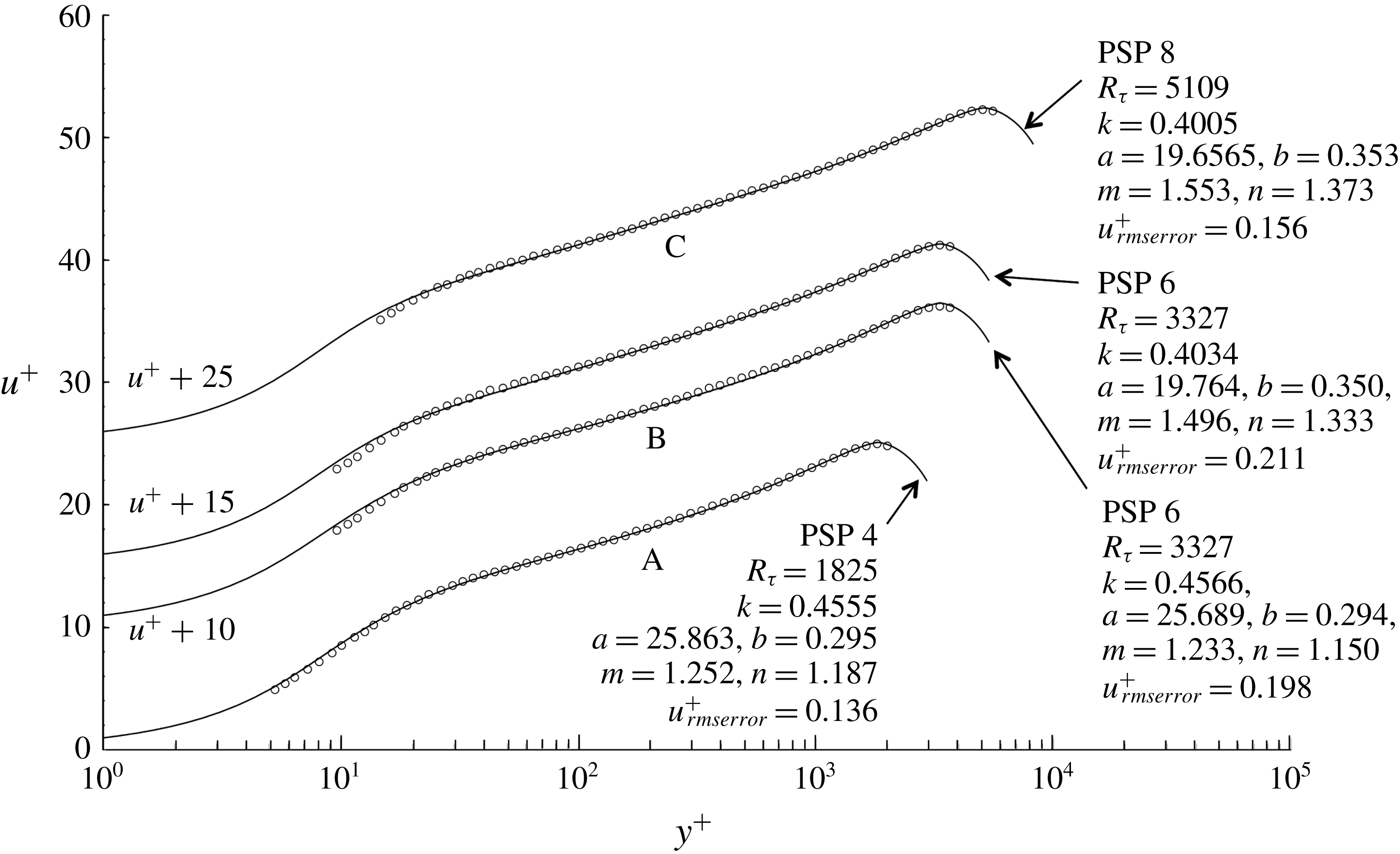
A note of caution needs to added here. Within the optimization procedure described in § 5, the value of
 $k$
that minimizes the squared error is quite well defined; in other words, small deviations from the optimum value of
 $k$
significantly increase the error in (5.1). However the optimization problem is not convex and multiple extrema in the squared error do exist. Figure 11 illustrates precisely this situation. Velocity surveys 4, 6 and 8 are shown along with the parameter values that define the model profile that best fits each survey. Survey 6, which has the largest error over the whole set of 26 PSP surveys, is shown twice with two sets of quite different optimal parameters that give almost exactly the same root-mean-square error in
 $u^{+}$
between the survey data and the model profile. The labels
 $\text{A}$
,
 $\text{B}$
and
 $\text{C}$
are placed near the section of each survey that would normally be associated with logarithmic behaviour. The model profile fit to survey 4 shows a concave section near
 $\text{A}$
that, in linear coordinates, would roughly correspond to dependence of the velocity profile on a power law. The intermediate region
 $\text{C}$
of survey 8 shows a straightening out of both the survey 8 data and the model profile and marks the beginning, in Reynolds number, of scale separation and nearly logarithmic behaviour in the intermediate region. Survey 6 falls somewhere in between. The model profile with
 $k=0.4566$
shows concave upward behaviour in the intermediate region
 $\text{B}$
and does not provide a very good fit to the survey 6 data in this region; this profile fits the data below
 $y^{+}=100$
better. The profile fit with
 $k=0.4034$
has less concave upward behaviour in the intermediate region and fits the data near
 $\text{B}$
better but this profile fits the data below
 $y^{+}=100$
less well. Because of the better fit to the data in region
 $\text{B}$
, the profile with
 $k=0.4034$
and the associated values of
 $a$
,
 $b$
,
 $m$
and
 $n$
was the one selected to be included in table 1. A search for similar cases of multiple extrema near profiles 1 to 5 and 7 to 26 did not turn up any other examples but that does not mean they do not exist. In the face of this uncertainty, the best reassurance that the parameter values presented in table 1 are of practical use is simply the fact that the errors are small and the fit to the data shown in figure 7 is generally very good.
Figure 12 shows the velocity gradient function (3.3) used to generate the universal model velocity profiles with optimal parameters used in the wall–wake mixing length function (3.13). Panel (a) is plotted in log–linear coordinates with the inset in linear coordinates to show the limiting gradient of the profile near
 $y^{+}=0$
derived in equation (3.4). In (b) the gradient is plotted in log–log coordinates to bring out the behaviour in the wake region. The rapid drop-off at the pipe centreline is essentially graphical evidence of the integrability of (3.3). Figure 12 also shows the difficulty of integrating (3.3) at high Reynolds number where the gradient near the pipe centreline is extremely small. This is a problem we will address later when we study the behaviour of the velocity profile expressed in outer variables at extreme Reynolds numbers.
The velocity gradient of the universal profile, equation (3.3). (a) Log–linear coordinates with linear inset; (b) log–log coordinates.

6.1 Velocity and friction using mean model parameters
The average value of
 $k$
in figure 8(b) over profiles 6 to 26 is
 $\bar{k}=0.4092$
and can be compared to the value
 $k=0.421$
measured by McKeon (Reference McKeon2003) and McKeon et al. (Reference McKeon, Zagarola and Smits2005) and
 $k=0.436$
reported by Zagarola (Reference Zagarola1996) and Zagarola & Smits (Reference Zagarola and Smits1998). The difference between 0.436 and 0.409 may not seem very large but to anyone fitting this kind of data to a logarithmic curve, the difference is quite noticeable and Zagarola’s value has generally been viewed as too large. But according to figure 2 the PSP survey data for
 $u_{0}/u_{\unicode[STIX]{x1D70F}}$
versus
 $R_{\unicode[STIX]{x1D70F}}$
are well approximated using
 $k=0.432$
, even though this value does not provide a good fit to any of the individual velocity profiles. We shall return to this point in § 9.3.
Table 1 shows the optimal values of (
 $k,a,b,m,n$
) determined for the 26 surveys. For PSP 1 to 5 the damping length scale
 $a$
is nearly constant around a value of approximately 25.7. At PSP 6,
 $a$
drops to 19.7, then increases slightly over PSP 6 to 21 and then levels off for PSP 22 to 26. The average value over PSP 6 to 26 is
 $\bar{a}=20.095$
. Over the entire data set the outer flow length scale,
 $b$
, shown in figure 10(b), is close to 0.3 except for a slight rise to approximately 0.34 to 0.35 between PSP 6 to 10. The average over PSP 6 to 26 is
 $\bar{b}=0.3195$
. The damping exponent,
 $m$
, shown in 10(c) shows similar behaviour; nearly constant at approximately 1.3 for PSP 1 to 5, then increasing to approximately 1.6 for PSP 6 to 26 with an average value
 $\bar{m}=1.621$
over these cases. Finally the wake exponent,
 $n$
, in figure 10(d) generally increases from 1.2 to 1.7 over PSP 1 to 26 with an average value over PSP 6 to 26 of
 $\bar{n}=1.619$
, remarkably close to
 $\bar{m}$
.


(a) Value of
 $\bar{u}/u_{\unicode[STIX]{x1D70F}}$
versus
 $R_{\unicode[STIX]{x1D70F}}$
, (b)
 $\bar{u}/u_{\unicode[STIX]{x1D70F}}$
versus
 $\bar{R}_{e}$
. Open circles, (○) are the combined Oregon and Princeton data from McKeon et al. (Reference McKeon, Swanson, Zagarola, Donnelly and Smits2004b
). Filled circles (●) are computed from (3.5) and (3.13) using
 $(\bar{k},\bar{a},\bar{m},\bar{b},\bar{n})=(0.4092,20.095,1.621,0.3195,1.619)$
.

Figure 13 shows the 26 sets of PSP survey velocity data as open circles and the comparison model profiles as solid lines. These are the same data shown in figure 7. The filled circles overlaid on the data are derived from the model profile with all five parameters fixed at their average values,
 $(\bar{k},\bar{a},\bar{m},\bar{b},\bar{n})=(0.4092,20.095,1.621,0.3195,1.619)$
. The fit is quite good considering the three orders of magnitude in the Reynolds number between surveys 1 and 26. The largest error occurs at the highest Reynolds number where the filled circles tend to overestimate the velocity. This is mainly due to the use of
 $\bar{k}=0.4092$
rather than the somewhat larger optimal value
 $k=0.4190$
.
In figure 14,
 $\bar{u}/u_{\unicode[STIX]{x1D70F}}$
versus
 $R_{\unicode[STIX]{x1D70F}}$
and the bulk Reynolds number,
 $\bar{R_{e}}$
, for the combined Oregon and Princeton data listed in McKeon et al. (Reference McKeon, Swanson, Zagarola, Donnelly and Smits2004b
), is compared with data computed from the universal velocity profile (3.5), (3.13) with the model parameters fixed at their average values. Except for laminar–turbulent transition, the universal profile approximates the friction data quite well over the entire range of Reynolds numbers from
 $0$
to
 $10^{7}$
.
7 Discussion
7.1 Logarithmic behaviour
At this point we have established that the model velocity profile (3.5) and (3.13) with optimal values of
 $(k,a,b,m,n)$
, provides an accurate approximation to the entire set of 26 surveys. In order to identify logarithmic behaviour, equations (3.3) and (3.13) are now combined to produce the log-law indicator function,
 $y^{+}\,\text{d}u^{+}/\text{d}y^{+}$
.
 $$\begin{eqnarray}\displaystyle y^{+}\frac{\text{d}u^{+}}{\text{d}y^{+}} & = & \displaystyle \frac{\left(1+\left(\displaystyle \frac{y^{+}}{bR_{\unicode[STIX]{x1D70F}}}\right)^{n}\right)^{2/n}}{2k^{2}y^{+}\left(1-\text{e}^{-(y^{+}/a)^{m}}\right)^{2}}\nonumber\\ \displaystyle & & \displaystyle \times \left(-1+\left(1+4(ky^{+})^{2}\frac{(1-\text{e}^{-(y^{+}/a)^{m}})^{2}}{\left(1+\left(\displaystyle \frac{y^{+}}{bR_{\unicode[STIX]{x1D70F}}}\right)^{n}\right)^{2/n}}\left(1-\frac{y^{+}}{R_{\unicode[STIX]{x1D70F}}}\right)\right)^{1/2}\right).\quad\end{eqnarray}$$
Comparison of the log-law indicator function for several sets of PSP model profiles. (a) PSP 1 to PSP 5, (b) PSP 6 to PSP 26, figure, (c) PSP 15 to 26. (d) Shows PSP profiles 15 to 26 on an expanded scale. Extrema of
 $y^{+}(\text{d}u^{+}/\text{d}y^{+})$
in (c) are identified by
 $\text{I}$
,
 $\text{II}$
,
 $\text{III}$
,
 $\text{IV}$
and
 $\text{V}$
. The arrow in (d) indicates the lowest Reynolds number appearance of the minimum
 $\text{IV}$
at PSP case 16.

Equation (7.1) is plotted in figure 15 for all 26 profiles. Profiles 1 to 5 are shown in figure 15(a), profiles 6 to 26 are shown in figure 15(b), the high Reynolds number profiles 15 to 26 are shown in figure 15(c) and an enlarged view of figure 15(c) is included as figure 15(d) in order to show the behaviour of the high Reynolds number profiles in the intermediate region. Each curve in figure 15 has several extrema and these are identified in figure 15(c,d). The outer edge of the viscous sublayer is defined here as the peak at
 $\text{I}$
. The outer edge of the buffer layer and beginning of the intermediate layer are defined as the minimum at
 $\text{II}$
. Every profile has a point
 $\text{III}$
in the middle of the wake region where
 $y^{+}\,\text{d}u^{+}/\text{d}y^{+}$
has a maximum just before the centre of the pipe is reached. Profiles 16 (
 $R_{\unicode[STIX]{x1D70F}}=42\,294$
) to 26 have a second minimum,
 $\text{IV}$
, one of which is identified by the arrow pointing at the minimum in profile 16 in figure 15(d). In these cases the minimum at
 $\text{IV}$
helps to identify the beginning of the wake region of the velocity profile. Profiles 16 to 26 also have a broad region,
 $\text{V}$
, with a maximum that defines the point where the profile would exactly fit a logarithm. At the highest PSP Reynolds number, the wake region begins at approximately
 $y^{+}=12\,000$
.
Despite the presence of the minimum around
 $y^{+}=100$
, there is really no log region in figure 15(a) for profiles 1 to 5 and, in effect, no scale separation below
 $R_{\unicode[STIX]{x1D70F}}=2345$
. The concave upward shape of the
 $y^{+}\,\text{d}u^{+}/\text{d}y^{+}$
curves is fairly marked throughout the intermediate region. El Khoury et al. (Reference El Khoury, Schlatter, Noorani, Fischer, Brethouwer and Johansson2013) in their figure 8(b) show comparisons of
 $y^{+}\,\text{d}u^{+}/\text{d}y^{+}$
determined from pipe, channel and boundary layer simulations at
 $R_{\unicode[STIX]{x1D70F}}\cong 1000$
. The curves are very similar to figure 15(a); the magnitude of the peak is slightly lower than the PSP 1 peak and the position at
 $y^{+}=10$
is slightly higher than the position of the peak at
 $y^{+}=8.3$
seen in 15. Similar pipe simulation results are shown in figure 4(b) of Ahn et al. (Reference Ahn, Lee, Lee, Kang and Sung2015) at
 $R_{\unicode[STIX]{x1D70F}}=3008$
.
Figure 15(b) shows model profiles 6 to 26. To a first approximation, a logarithm is an excellent fit in the nearly flat region that begins at
 $y^{+}=65$
, and reaches to the beginning of the wake region. Upon closer inspection, the slope of the straight section of each profile actually shows a small increase with
 $y^{+}$
. In order to examine this further, the high Reynolds number profiles 15 (
 $R_{\unicode[STIX]{x1D70F}}=32\,869$
) to 26 (
 $R_{\unicode[STIX]{x1D70F}}=530\,023$
) are broken out in figure 15(c,d). For PSP surveys 15 to 26 the log-law indicator function has a slightly concave downward shape in the nominally logarithmic region. Figure 15(d) shows that profiles 16,
 $R_{\unicode[STIX]{x1D70F}}=42\,294$
, to 26 have a second minimum
 $\text{IV}$
that defines the beginning of the wake region and distinct scale separation between the wall and the wake. It appears that
 $R_{\unicode[STIX]{x1D70F}}=42\,294$
is the Reynolds number where full separation of scales between the wall and wake is reached. There is no maximum in region
 $\text{V}$
in the model velocity profiles for PSP surveys 1 to 15; that is, there is no point where a log function would fit precisely despite the remarkable flatness of this region in figure 15(b). The presence of a maximum in region
 $\text{V}$
persists to all higher Reynolds numbers with an increasingly lengthy logarithmic section of the velocity profile. Perhaps the most accurate description of region
 $\text{V}$
is that the profile shape is not precisely a logarithm, but is the more complex behaviour defined by the universal velocity profile (3.5) and (3.13) with the influence of wall and outer length scales on the intermediate region of the velocity profile persisting to all Reynolds numbers.
7.2 Power-law behaviour
Using similarity arguments and experimental data, Barenblatt (Reference Barenblatt1993) and Barenblatt & Prostokishin (Reference Barenblatt and Prostokishin1993) argue that the intermediate region in wall-bounded flows, particularly pipe flow, is not governed by a universal logarithmic profile but rather by a Reynolds number dependent power law, apparently free of empirical constants, of the form
 $$\begin{eqnarray}\displaystyle u^{+}=\left(\frac{1}{\sqrt{3}}\ln (2\bar{R}_{e})+\frac{5}{2}\right)(y^{+})^{3/(2\ln (2\bar{R}_{e}))}, & & \displaystyle\end{eqnarray}$$
where
 $\bar{R}_{e}$
is the Reynolds number based on the bulk velocity and pipe radius.
We can check this hypothesis. The universal velocity profile with optimal parameters is used to construct the power-law indicator function
 $(y^{+}/u^{+})\text{d}u^{+}/\text{d}y^{+}$
for PSP cases 1 to 26 shown in figure 16(a). In all 26 cases the slope of the profile in figure 16(a) is negative until the minimum is reached beyond the outer edge of the intermediate region. Indeed, every curve in figure 16(a) has a minimum where a power law would provide a locally accurate fit. The values of
 $((y^{+}/u^{+})\text{d}u^{+}/\text{d}y^{+})_{min}$
(the exponents) at the minima are shown in figure 16(b) and the Reynolds number dependent exponent in (7.2) is shown for comparison. In figure 16(c) values of the coefficient in (7.2), determined for PSP cases 1 to 26 using the universal velocity profile and the exponent data in figure 16(b), are shown as open circles and compared with the coefficient in (7.2). The agreement between the data derived from the universal velocity profile and (7.2) for both the exponent and the coefficient is very good, although there is some systematic variation in both figures.
It must be noted that, while the functional form of (7.2) has a basis in fundamental theory, the constants in (7.2) are, in fact, empirically determined by Barenblatt & Prostokishin (Reference Barenblatt and Prostokishin1993) to provide the best fit to the pipe data of Nikuradse (Reference Nikuradse1966) over the range
 $8.35\times 10^{3}<\bar{R}_{e}<7.68\times 10^{5}$
. The low end of this range is below the Reynolds number of PSP 1. The high end lies between PSP 14 and 15 close to where the theoretical curves cross the data generated from the universal profile in figure 16(b,c). So the agreement in these figures is really just a reflection of the fact that the universal velocity profile and (7.2) are approximating pipe data from two different sources 64 years apart at the same flow conditions. The reason Barenblatt & Prostokishin (Reference Barenblatt and Prostokishin1993) expressed the constants in (7.2) in terms whole numbers was purely for convenience as they state in the discussion in § 2.2 of their paper.
Barenblatt (Reference Barenblatt1993) and Barenblatt & Prostokishin (Reference Barenblatt and Prostokishin1993) argue that (7.2) should replace the logarithmic profile in the intermediate region. However figure 16(d) shows that the minima in figure 16(a) are all located above
 $y/\unicode[STIX]{x1D6FF}=0.08$
, somewhere between the extrema labelled
 $\text{IV}$
and
 $\text{III}$
in figure 15(c). It appears that (7.2) is more descriptive of the transition region where the logarithm gives way to the outer flow rather than the intermediate region itself.
This issue is beginning to be within the range of direct numerical simulation. Ahn et al. (Reference Ahn, Lee, Lee, Kang and Sung2015) plot
 $(y^{+}/u^{+})\text{d}u^{+}/\text{d}y^{+}$
in their figure 4(a). A flat section indicates that the velocity profile in their simulation at
 $R_{\unicode[STIX]{x1D70F}}=3008$
follows a power law with exponent
 $0.145$
in the range
 $y^{+}=90$
–
 $300$
. This agrees reasonably well with the nearest comparable PSP case which would be survey 6 at
 $R_{\unicode[STIX]{x1D70F}}=3327$
. However at this Reynolds number there is very little scale separation between the wall and outer flow and so the log-law and power-law regions are very difficult to distinguish.
Power-law indicator function for the PSP model profile and comparison with the theoretical prediction of Barenblatt (Reference Barenblatt1993) and Barenblatt & Prostokishin (Reference Barenblatt and Prostokishin1993). (a) Shows model profiles PSP 1 to PSP 26. In (b), open circles (○) are the values of the exponent at the minima of the curves in (a), the solid line is the exponent in (7.2). In (c), open circles are determined from the universal velocity profile at the minima in (a) and the exponents in (b), the solid line is the coefficient in (7.2). (d) Indicates the position of the minima from (a) in outer flow coordinates.

7.3 Scaling of regions
$\text{I}$
,
$\text{II}$
,
$\text{III}$
,
$\text{IV}$
and
$\text{V}$


The collapse of the 26 velocity profiles in the viscous near wall region
 $\text{I}$
and
 $\text{II}$
in figure 15 is nearly perfect with a maximum value of
 $y^{+}\,\text{d}u^{+}/\text{d}y^{+}$
close to 6.0 at the edge of the viscous sublayer at
 $y^{+}=8.3$
and a minimum at the end of the viscous wall layer at
 $y^{+}=65$
.
To a high degree of accuracy, the
 $y^{+}$
position of the peak at
 $\text{III}$
scales linearly with
 $R_{\unicode[STIX]{x1D70F}}$
and
 $$\begin{eqnarray}\displaystyle \frac{y_{III}^{+}}{R_{\unicode[STIX]{x1D70F}}}=\frac{y_{III}}{\unicode[STIX]{x1D6FF}}=0.592\pm 0.012 & & \displaystyle\end{eqnarray}$$
over all 26 profiles. This is consistent with the remarkable constancy of the model parameter
 $b$
. It appears that the middle of the wake region is at approximately
 $y/\unicode[STIX]{x1D6FF}=2b$
. The
 $y^{+}$
position of the minimum at
 $\text{IV}$
, which we define as the beginning of the wake region, does not appear in the survey data until
 $R_{\unicode[STIX]{x1D70F}}=42\,294$
and relatively few survey data points are available to define the
 $R_{\unicode[STIX]{x1D70F}}$
scaling of this minimum. To remedy this, the universal profile was extrapolated to
 $R_{\unicode[STIX]{x1D70F}}=10^{8}$
with optimal parameters fixed at their mean values. For Reynolds numbers above
 $R_{\unicode[STIX]{x1D70F}}=42\,294$
up to
 $R_{\unicode[STIX]{x1D70F}}\cong 10^{8}$
the minimum at
 $\text{IV}$
also scales linearly with
 $R_{\unicode[STIX]{x1D70F}}$
and
 $$\begin{eqnarray}\displaystyle \frac{y_{IV}^{+}}{R_{\unicode[STIX]{x1D70F}}}=\frac{y_{IV}}{\unicode[STIX]{x1D6FF}}=0.0149\pm 0.0008. & & \displaystyle\end{eqnarray}$$
The
 $y^{+}$
position of the maximum in region
 $\text{V}$
that defines the point where a logarithm would be an exact fit was determined by solving for the positive real root of
 $\text{d}(y^{+}\,\text{d}u^{+}/\text{d}y^{+})\,\text{d}y^{+}=0$
. The maximum is quite broad and over the Reynolds number range of the PSP data it is difficult to precisely identify a simple scaling. However, when the universal profile was extrapolated to
 $R_{\unicode[STIX]{x1D70F}}\cong 10^{8}$
with parameters fixed at their mean values, the scaling was found to be
 $$\begin{eqnarray}\displaystyle \frac{y_{V}^{+}}{\left(\displaystyle \frac{R_{\unicode[STIX]{x1D70F}}}{k}\right)^{1/2}}\cong 1. & & \displaystyle\end{eqnarray}$$
The result (7.5) coincides quite closely to the point of maximum turbulent shear stress (7.14) at high Reynolds numbers. Note that a maximum in
 $\unicode[STIX]{x1D70F}^{+}$
exists at all Reynolds numbers whereas region
 $\text{V}$
only has a maximum for PSP survey 16,
 $R_{\unicode[STIX]{x1D70F}}>42\,294$
, and above.
7.4 The Reynolds shear stress and turbulent kinetic energy production
The universal velocity profile (3.5) and (3.13) can be used to analyse turbulent shear stress profiles from the pipe centreline to the wall. This inevitably requires discussion of the implications of the approximate profile in the near-wall region well below, in logarithmic terms, the nearest data point used to generate the profile. The discussion in this section needs to be understood in this light: despite the absence of data very near the wall, what does the PSP data seem to suggest about the near-wall flow?
Turbulent shear stress profiles are shown in figure 17. As the Reynolds number increases, the
 $y^{+}$
coordinate of the maximum stress increases while the value of the maximum stress approaches one corresponding to the classical high Reynolds number approximation
 $(\overline{u^{\prime }v^{\prime }})_{max}\cong -\unicode[STIX]{x1D70F}_{wall}/\unicode[STIX]{x1D70C}$
.
Turbulent shear stress profiles using optimal parameter values for each profile; (a) all 26 surveys, (b) shear stress very near the wall in log–log coordinates.

From (2.9) and (3.3) the turbulent shear stress is
 $$\begin{eqnarray}\displaystyle \unicode[STIX]{x1D70F}^{+}=\left(1-\frac{y^{+}}{R_{\unicode[STIX]{x1D70F}}}\right)+\frac{1}{2\unicode[STIX]{x1D706}(y^{+})^{2}}-\frac{1}{2\unicode[STIX]{x1D706}(y^{+})^{2}}\left(1+4\unicode[STIX]{x1D706}(y^{+})^{2}\left(1-\frac{y^{+}}{R_{\unicode[STIX]{x1D70F}}}\right)\right)^{1/2}. & & \displaystyle\end{eqnarray}$$
Extrema in the Reynolds shear stress occur where
 $$\begin{eqnarray}\displaystyle & & \displaystyle \frac{\text{d}\unicode[STIX]{x1D70F}^{+}}{\text{d}y^{+}}=0\Rightarrow \nonumber\\ \displaystyle & & \displaystyle \quad -\,\frac{1}{R_{\unicode[STIX]{x1D70F}}}+\frac{1}{R_{\unicode[STIX]{x1D70F}}\left(1+4\unicode[STIX]{x1D706}^{2}\left(1-\displaystyle \frac{y^{+}}{R_{\unicode[STIX]{x1D70F}}}\right)\right)^{1/2}}-\frac{1}{\unicode[STIX]{x1D706}^{3}}\frac{\text{d}\unicode[STIX]{x1D706}}{\text{d}y^{+}}-\frac{2}{\unicode[STIX]{x1D706}\left(1+4\unicode[STIX]{x1D706}^{2}\left(1-\displaystyle \frac{y^{+}}{R_{\unicode[STIX]{x1D70F}}}\right)\right)^{1/2}}\frac{\text{d}\unicode[STIX]{x1D706}}{\text{d}y^{+}}\nonumber\\ \displaystyle & & \displaystyle \quad +\,\frac{2y^{+}}{R_{\unicode[STIX]{x1D70F}}\unicode[STIX]{x1D706}\left(1+4\unicode[STIX]{x1D706}^{2}\left(1-\displaystyle \frac{y^{+}}{R_{\unicode[STIX]{x1D70F}}}\right)\right)^{1/2}}\frac{\text{d}\unicode[STIX]{x1D706}}{\text{d}y^{+}}+\frac{1}{\unicode[STIX]{x1D706}^{3}}\left(1+4\unicode[STIX]{x1D706}^{2}\left(1-\frac{y^{+}}{R_{\unicode[STIX]{x1D70F}}}\right)\right)^{1/2}\frac{\text{d}\unicode[STIX]{x1D706}}{\text{d}y^{+}}=0.\end{eqnarray}$$
Equation (7.7) can be squared and rearranged to read
 $$\begin{eqnarray}\displaystyle \frac{4}{{R_{\unicode[STIX]{x1D70F}}}^{2}\unicode[STIX]{x1D706}^{2}}\left(1-\frac{y^{+}}{R_{\unicode[STIX]{x1D70F}}}\right)\left({R_{\unicode[STIX]{x1D70F}}}^{2}\left(1-\frac{y^{+}}{R_{\unicode[STIX]{x1D70F}}}\right)\left(\frac{\text{d}\unicode[STIX]{x1D706}}{\text{d}y^{+}}\right)^{2}-R_{\unicode[STIX]{x1D70F}}\unicode[STIX]{x1D706}\frac{\text{d}\unicode[STIX]{x1D706}}{\text{d}y^{+}}-\unicode[STIX]{x1D706}^{4}\right)=0. & & \displaystyle\end{eqnarray}$$
The zero of (7.8) at
 $y^{+}=R_{\unicode[STIX]{x1D70F}}$
is a spurious root introduced by the squaring process. The factor of interest is
 $$\begin{eqnarray}\displaystyle {R_{\unicode[STIX]{x1D70F}}}^{2}\left(1-\frac{y^{+}}{R_{\unicode[STIX]{x1D70F}}}\right)\left(\frac{\text{d}\unicode[STIX]{x1D706}_{max\unicode[STIX]{x1D70F}^{+}}}{\text{d}y^{+}}\right)^{2}-R_{\unicode[STIX]{x1D70F}}(\unicode[STIX]{x1D706}_{max\unicode[STIX]{x1D70F}^{+}})\frac{\text{d}\unicode[STIX]{x1D706}_{max\unicode[STIX]{x1D70F}^{+}}}{\text{d}y^{+}}-(\unicode[STIX]{x1D706}_{max\unicode[STIX]{x1D70F}^{+}})^{4}=0, & & \displaystyle\end{eqnarray}$$
where
 $\unicode[STIX]{x1D70F}^{+}$
is a maximum and
 $\unicode[STIX]{x1D706}_{max\unicode[STIX]{x1D70F}^{+}}$
is the value of
 $\unicode[STIX]{x1D706}$
at the maximum. Recall
 $\unicode[STIX]{x1D702}=(1-y/\unicode[STIX]{x1D6FF})=(1-y^{+}/R_{\unicode[STIX]{x1D70F}})$
, equation (7.9) becomes
 $$\begin{eqnarray}\displaystyle \left(\frac{\text{d}\unicode[STIX]{x1D706}_{max\unicode[STIX]{x1D70F}^{+}}}{\text{d}\unicode[STIX]{x1D702}}\right)^{2}+\frac{(\unicode[STIX]{x1D706}_{max\unicode[STIX]{x1D70F}^{+}})}{\unicode[STIX]{x1D702}}\frac{\text{d}\unicode[STIX]{x1D706}_{max\unicode[STIX]{x1D70F}^{+}}}{\text{d}\unicode[STIX]{x1D702}}-\frac{(\unicode[STIX]{x1D706}_{max\unicode[STIX]{x1D70F}^{+}})^{4}}{\unicode[STIX]{x1D702}}=0. & & \displaystyle\end{eqnarray}$$
Equation (7.10) can be solved for
 $\unicode[STIX]{x1D706}_{max\unicode[STIX]{x1D70F}^{+}}$
.
 $$\begin{eqnarray}\displaystyle \unicode[STIX]{x1D706}_{max\unicode[STIX]{x1D70F}^{+}}=\frac{1}{2\left(1-\displaystyle \frac{y_{max\unicode[STIX]{x1D70F}^{+}}^{+}}{R_{\unicode[STIX]{x1D70F}}}\right)^{1/2}}\left(\left(\frac{(1+\text{const.})-\text{const.}\displaystyle \frac{y_{max\unicode[STIX]{x1D70F}^{+}}^{+}}{R_{\unicode[STIX]{x1D70F}}}}{(1-\text{const.})+\text{const.}\displaystyle \frac{y_{max\unicode[STIX]{x1D70F}^{+}}^{+}}{R_{\unicode[STIX]{x1D70F}}}}\right)^{2}-1\right)^{1/2}, & & \displaystyle\end{eqnarray}$$
where
 $\text{const.}$
is the positive,
 $R_{\unicode[STIX]{x1D70F}}$
dependent, constant of integration of (7.10). Equation (7.11) simplifies to
 $$\begin{eqnarray}\displaystyle \unicode[STIX]{x1D706}_{max\unicode[STIX]{x1D70F}^{+}}=\frac{\text{const.}^{1/2}}{\left((1-\text{const.})+\text{const.}\displaystyle \frac{y_{max\unicode[STIX]{x1D70F}^{+}}^{+}}{R_{\unicode[STIX]{x1D70F}}}\right)}. & & \displaystyle\end{eqnarray}$$
Once the mixing length function,
 $\unicode[STIX]{x1D706}(y^{+})$
, is defined, equation (7.12) can be solved for the value of
 $y^{+}$
where
 $\unicode[STIX]{x1D70F}^{+}$
is a maximum.
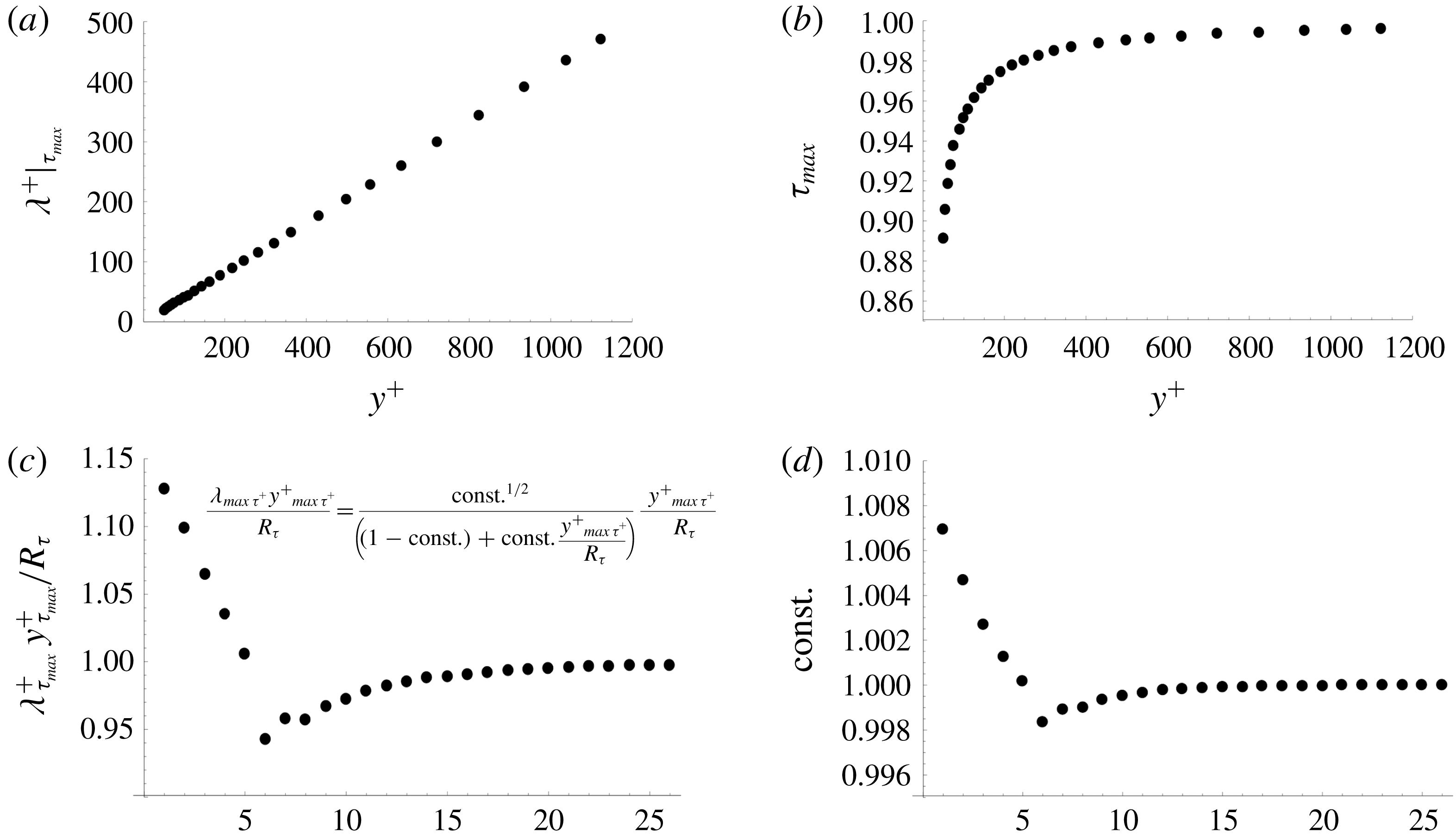
Figure 18 shows the position above the wall as well as the value of the maximum turbulent shear stress derived from the model profiles for PSP 1 to 26. At high Reynolds number, the maximum
 $\unicode[STIX]{x1D70F}^{+}$
approaches one. The position of maximum turbulent shear stress is always far below the wake region and, for PSP surveys 15 to 26, the position of maximum shear stress is far enough outside the wall damping region so that to a good approximation,
 $$\begin{eqnarray}\displaystyle \left.\begin{array}{@{}c@{}}\unicode[STIX]{x1D706}_{max\unicode[STIX]{x1D70F}^{+}}^{+}\cong ky_{max\unicode[STIX]{x1D70F}^{+}}^{+}\\ \text{const.}\cong 1.\end{array}\right\} & & \displaystyle\end{eqnarray}$$
According to (7.12) and (7.13), the position of the point of maximum turbulent shear stress increases with Reynolds number as,
 $$\begin{eqnarray}\displaystyle y_{max\unicode[STIX]{x1D70F}^{+}}^{+}\cong \sqrt{\frac{R_{\unicode[STIX]{x1D70F}}}{k}} & & \displaystyle\end{eqnarray}$$
in agreement with equation (42) in Zagarola & Smits (Reference Zagarola and Smits1998) and consistent with the conclusions of Morrill-Winter et al. (Reference Morrill-Winter, Phillip and Klewicki2017) in the context of flat plate flow. Finally, very near the wall, equation (7.6) can be expanded to give,
 $$\begin{eqnarray}\displaystyle \lim _{y^{+}\rightarrow 0}\unicode[STIX]{x1D70F}^{+}=\left(\frac{k^{2}}{4a^{2m}}\right)(y^{+})^{2+2m}. & & \displaystyle\end{eqnarray}$$
The average value of the damping exponent over PSP 6 to 26 is
 $\bar{m}=1.621$
, corresponding to
 $2\bar{m}+2=5.242$
. In figure 17(b), the shear stress profiles are plotted in log–log coordinates to show the behaviour of the model profiles very near the wall. The small variation in slopes in figure 17(b) reflects the variation in
 $m$
over the 26 profiles. The profiles indicate that near the wall,
 $\unicode[STIX]{x1D70F}^{+}\sim (y^{+})^{5}$
in contrast to generally accepted thinking and the analysis and simulation results of She et al. (Reference She, Chen and Hussain2017). The result in (7.15) is consistent with the rapidly damped near-wall flow observed in the model velocity profiles in figure 7 as well as the position of the near-wall peak in the streamwise normal stress data presented in Hultmark (Reference Hultmark2012). It should be noted that if the uncorrected Zagarola (Reference Zagarola1996) data are analysed using the approach here with optimal parameters appropriate to that data set, the near-wall Reynolds stress does behave as
 $\unicode[STIX]{x1D70F}^{+}\sim (y^{+})^{3}$
.
(a) Mixing length function
 $\unicode[STIX]{x1D706}$
normalized by
 $ky^{+}$
. (b,c) Turbulent kinetic energy production,
 $P^{+}=\unicode[STIX]{x1D70F}^{+}(\text{d}u^{+}/\text{d}y^{+})$
, in log–linear coordinates and log–log coordinates respectively. (d) Area-averaged TKE production multiplied by
 $R_{\unicode[STIX]{x1D70F}}$
. The root-mean-square error in the log–linear fit to the data in (d) is 0.175. All 26 profiles are shown with optimal parameters used for each profile.

The normalized mixing length function
 $\unicode[STIX]{x1D706}/ky^{+}$
for corrected PSP surveys 1 to 26 is shown in figure 19(a). There is no flat region for model profiles 1 to 5. Profiles 6 to 26 show the same, very regular, behaviour seen in figure 15. There is a notable gap between the mixing length functions for PSP cases 5 and 6. This reflects the step in the value of the optimal
 $k$
for these cases seen in figure 9 that, as was noted in § 6, may be evidence of a mixing transition between these cases.
Figure 19(b,c) shows the production of turbulent kinetic energy (TKE). Returning to (2.9), multiply by
 $\text{d}u^{+}/\text{d}y^{+}$
to produce
 $$\begin{eqnarray}\displaystyle \unicode[STIX]{x1D70F}^{+}\frac{\text{d}u^{+}}{\text{d}y^{+}}=\left(1-\frac{y^{+}}{R_{\unicode[STIX]{x1D70F}}}\right)\frac{\text{d}u^{+}}{\text{d}y^{+}}-\left(\frac{\text{d}u^{+}}{\text{d}y^{+}}\right)^{2}. & & \displaystyle\end{eqnarray}$$
The left-hand side of (7.16) is the TKE production. Differentiate (7.16), set the result to zero and take the limit
 $R_{\unicode[STIX]{x1D70F}}\rightarrow \infty$
.
 $$\begin{eqnarray}\displaystyle \lim _{R_{\unicode[STIX]{x1D70F}}\rightarrow \infty }\left(-\frac{1}{R_{\unicode[STIX]{x1D70F}}}\frac{\text{d}u^{+}}{\text{d}y^{+}}+\left(1-\frac{y^{+}}{R_{\unicode[STIX]{x1D70F}}}-2\left(\frac{\text{d}u^{+}}{\text{d}y^{+}}\right)\right)\frac{\text{d}^{2}u^{+}}{\text{d}(y^{+})^{2}}\right)=\left(1-2\left(\frac{\text{d}u^{+}}{\text{d}y^{+}}\right)\right)\frac{\text{d}^{2}u^{+}}{\text{d}(y^{+})^{2}}=0. & & \displaystyle \nonumber\\ \displaystyle & & \displaystyle\end{eqnarray}$$
At high Reynolds number, the maximum TKE production occurs where
 $\text{d}u^{+}/\text{d}y^{+}=1/2$
(and
 $\unicode[STIX]{x1D70F}^{+}=1/2$
). Plugging this result into (7.16), the maximum in the turbulent kinetic energy production is
 $(\unicode[STIX]{x1D70F}^{+}(\text{d}u^{+}/\text{d}y^{+}))_{max}=1/4$
. The maximum occurs at
 $y^{+}=12$
(Chen, Hussain & She Reference Chen, Hussain and She2018), somewhat above the outer edge of the viscous sublayer as can be seen in figure 19(b). Figure 19(c) shows the TKE production in log–log coordinates and is intended to provide some insight into the behaviour of the TKE production away from the wall region. This figure illustrates the decrease in production in the outer layer and, to a degree, the relative proportion of production near the wall versus the outer layer. To explore this further, the TKE production is area averaged over the pipe,
 $$\begin{eqnarray}\displaystyle \overline{P^{+}}=\frac{2}{R_{\unicode[STIX]{x1D70F}}}\int _{0}^{R_{\unicode[STIX]{x1D70F}}}P^{+}\left(1-\frac{y^{+}}{R_{\unicode[STIX]{x1D70F}}}\right)\text{d}y^{+}, & & \displaystyle\end{eqnarray}$$
where
 $\overline{P^{+}}=\overline{P}\unicode[STIX]{x1D708}/u_{\unicode[STIX]{x1D70F}}^{4}$
. The result, equation (7.18), multiplied by
 $R_{\unicode[STIX]{x1D70F}}$
is shown in figure 19(d). According to the universal model profile the area-averaged production of turbulent kinetic energy decreases with Reynolds number according to
 $$\begin{eqnarray}\displaystyle \overline{P^{+}}=\frac{4.620\ln (R_{\unicode[STIX]{x1D70F}})-12.871}{R_{\unicode[STIX]{x1D70F}}}. & & \displaystyle\end{eqnarray}$$
The implication of this result is that in the limit of infinite Reynolds number, the area-averaged production of TKE tends to 0. This agrees generally with the analysis of Pullin et al. (Reference Pullin, Inoue and Saito2013) and is consistent with the decrease with Reynolds number of the velocity gradient in the outer flow.
The transport equation for the turbulent kinetic energy implies that, in general, TKE production and dissipation scale together
 $$\begin{eqnarray}\displaystyle \unicode[STIX]{x1D70F}\frac{\text{d}u}{\text{d}y}\simeq 2\unicode[STIX]{x1D708}\overline{({S_{ij}}^{\prime })({S_{ij}}^{\prime })}, & & \displaystyle\end{eqnarray}$$
where
 ${S_{ij}}^{\prime }$
is the fluctuating rate of strain. In wall variables, equation (7.20) becomes
 $$\begin{eqnarray}\displaystyle \unicode[STIX]{x1D70F}^{+}\frac{\text{d}u^{+}}{\text{d}y^{+}}=P^{+}\simeq 2\overline{({S_{ij}}^{\prime })^{+}({S_{ij}}^{\prime })^{+}}. & & \displaystyle\end{eqnarray}$$
The production of TKE normalized by the friction velocity in figure 19(b) remains invariant as the Reynolds number is increased. The normalized rate-of-strain fluctuation in (7.21) is related to the physical rate-of-strain fluctuation by
 $$\begin{eqnarray}\displaystyle ({S_{ij}}^{\prime })^{+}=\frac{{S_{ij}}^{\prime }\unicode[STIX]{x1D708}}{u_{\unicode[STIX]{x1D70F}}^{2}}. & & \displaystyle\end{eqnarray}$$
The problem here is that, at fixed
 $u_{0}$
and
 $\unicode[STIX]{x1D6FF}$
, as
 $\unicode[STIX]{x1D708}\rightarrow 0$
so also
 $u_{\unicode[STIX]{x1D70F}}\rightarrow 0$
. We know that
 $\unicode[STIX]{x1D708}/u_{\unicode[STIX]{x1D70F}}\rightarrow 0$
, but we also need to determine
 $\lim _{\unicode[STIX]{x1D708}\rightarrow 0}\unicode[STIX]{x1D708}/u_{\unicode[STIX]{x1D70F}}^{2}$
. Using the pipe friction law in the form
 $ku_{0}/u_{\unicode[STIX]{x1D70F}}=\ln (e^{C}u_{\unicode[STIX]{x1D70F}}\unicode[STIX]{x1D6FF}/\unicode[STIX]{x1D708})$
to express
 $\unicode[STIX]{x1D708}/u_{\unicode[STIX]{x1D70F}}^{2}$
in terms of
 $ku_{0}/u_{\unicode[STIX]{x1D70F}}$
,
 $$\begin{eqnarray}\displaystyle \frac{\unicode[STIX]{x1D708}}{u_{\unicode[STIX]{x1D70F}}^{2}}=\left(\frac{\text{e}^{C}\unicode[STIX]{x1D6FF}}{ku_{0}}\right)\left(\frac{ku_{0}}{u_{\unicode[STIX]{x1D70F}}}\right)\text{e}^{-(ku_{0}/u_{\unicode[STIX]{x1D70F}})}. & & \displaystyle\end{eqnarray}$$
In (7.23),
 $\unicode[STIX]{x1D6FF}$
and
 $u_{0}$
are fixed. As
 $ku_{0}/u_{\unicode[STIX]{x1D70F}}\rightarrow \infty$
the ratio
 $\unicode[STIX]{x1D708}/u_{\unicode[STIX]{x1D70F}}^{2}\rightarrow 0$
. Therefore, for fixed
 $\sqrt{\overline{({S_{ij}}^{\prime })^{+}({S_{ij}}^{\prime })^{+}}}$
,
 $$\begin{eqnarray}\displaystyle \lim _{\unicode[STIX]{x1D708}/u_{\unicode[STIX]{x1D70F}}^{2}\rightarrow 0}\sqrt{\overline{({S_{ij}}^{\prime })({S_{ij}}^{\prime })}}=\sqrt{\overline{({S_{ij}}^{\prime })^{+}({S_{ij}}^{\prime })^{+}}}\left(\frac{u_{\unicode[STIX]{x1D70F}}^{2}}{\unicode[STIX]{x1D708}}\right)\rightarrow \infty . & & \displaystyle\end{eqnarray}$$
As
 $\unicode[STIX]{x1D708}\rightarrow 0$
, the instantaneous velocity gradients within the viscous wall layer become infinite in order to maintain the balance (7.21).
8 High Reynolds number velocity profiles
Recall (3.5) and (3.13) repeated here for convenience with the full dependence on (
 $k,a,m,b,n,R_{\unicode[STIX]{x1D70F}}$
) shown.
 $$\begin{eqnarray}\displaystyle u^{+}(k,a,m,b,n,R_{\unicode[STIX]{x1D70F}},y^{+})=\int _{0}^{y^{+}}\left(-\frac{1}{2\unicode[STIX]{x1D706}^{2}}+\frac{1}{2\unicode[STIX]{x1D706}^{2}}\left(1+4\unicode[STIX]{x1D706}^{2}\left(1-\frac{s}{R_{\unicode[STIX]{x1D70F}}}\right)\right)^{1/2}\right)\text{d}s, & & \displaystyle\end{eqnarray}$$
where
 $$\begin{eqnarray}\displaystyle \unicode[STIX]{x1D706}(k,a,m,b,n,R_{\unicode[STIX]{x1D70F}},y^{+})=\frac{ky^{+}(1-\text{e}^{-(y^{+}/a)^{m}})}{\left(1+\left(\displaystyle \frac{y^{+}}{bR_{\unicode[STIX]{x1D70F}}}\right)^{n}\right)^{1/n}}. & & \displaystyle\end{eqnarray}$$
Equations (8.1) and (8.2) admit an interesting scaling. Use the group,
 $u/u_{0}\rightarrow ku/u_{0}$
,
 $y^{+}\rightarrow ky^{+}$
, and
 $R_{\unicode[STIX]{x1D70F}}\rightarrow kR_{\unicode[STIX]{x1D70F}}$
to define a modified wall–wake mixing length function by multiplying and dividing various terms in (8.2) by
 $k$
.
 $$\begin{eqnarray}\displaystyle \unicode[STIX]{x1D706}(k,a,m,b,n,R_{\unicode[STIX]{x1D70F}},y^{+}) & = & \displaystyle \frac{ky^{+}(1-\text{e}^{-(y^{+}/a)^{m}})}{\left(1+\left(\displaystyle \frac{y^{+}}{bR_{\unicode[STIX]{x1D70F}}}\right)^{n}\right)^{1/n}}=\frac{ky^{+}(1-\text{e}^{-(ky^{+}/ka)^{m}})}{\left(1+\left(\displaystyle \frac{ky^{+}}{b(kR_{\unicode[STIX]{x1D70F}})}\right)^{n}\right)^{1/n}}\nonumber\\ \displaystyle & = & \displaystyle \tilde{\unicode[STIX]{x1D706}}(ka,m,b,n,kR_{\unicode[STIX]{x1D70F}},ky^{+}).\end{eqnarray}$$
In the reduced space
 $k$
and
 $a$
are not independent parameters. Multiply both sides of (8.1) by
 $k$
, which is at most a function of
 $R_{\unicode[STIX]{x1D70F}}$
, and insert the modified mixing length function (8.3). Choose the integration variable,
 $\unicode[STIX]{x1D6FC}=ky^{+}$
.
 $$\begin{eqnarray}\displaystyle ku^{+}=\int _{0}^{ky^{+}}\left(-\frac{1}{2\tilde{\unicode[STIX]{x1D706}}^{2}}+\frac{1}{2\tilde{\unicode[STIX]{x1D706}}^{2}}\left(1+4\tilde{\unicode[STIX]{x1D706}}^{2}\left(1-\frac{\unicode[STIX]{x1D6FC}}{kR_{\unicode[STIX]{x1D70F}}}\right)\right)^{1/2}\right)\text{d}\unicode[STIX]{x1D6FC}. & & \displaystyle\end{eqnarray}$$
Equation (8.4) can be viewed as a
 $k$
independent model velocity profile with four model parameters, (
 $ka,m,b,n$
) in a pipe flow at the scaled friction Reynolds number,
 $kR_{\unicode[STIX]{x1D70F}}$
. Now, define the pipe flow shape function
 $$\begin{eqnarray}\displaystyle \unicode[STIX]{x1D6F7}(ka,b,m,n,kR_{\unicode[STIX]{x1D70F}},ky^{+})=\int _{0}^{ky^{+}}\!\left(-\frac{1}{2\tilde{\unicode[STIX]{x1D706}}^{2}}+\frac{1}{2\tilde{\unicode[STIX]{x1D706}}^{2}}\left(1+4\tilde{\unicode[STIX]{x1D706}}^{2}\left(1-\frac{\unicode[STIX]{x1D6FC}}{kR_{\unicode[STIX]{x1D70F}}}\right)\right)^{1/2}\right)\text{d}\unicode[STIX]{x1D6FC}-\ln (ky^{+}). & & \displaystyle \nonumber\\ \displaystyle & & \displaystyle\end{eqnarray}$$
(a) Pipe flow shape function,
 $\unicode[STIX]{x1D6F7}$
, versus
 $kR_{\unicode[STIX]{x1D70F}}$
with
 $y/\unicode[STIX]{x1D6FF}$
constant and
 $(ka,m,b,n)=(0.4092\times 20.095,1.621,0.3195,1.619)$
. (b) High Reynolds number limiting shape function,
 $\unicode[STIX]{x1D719}$
, versus
 $y/\unicode[STIX]{x1D6FF}$
. In (b), optimal parameter values are used for each curve.

Recall that
 $ky^{+}=(y/\unicode[STIX]{x1D6FF})kR_{\unicode[STIX]{x1D70F}}$
. The shape function, equation (8.5), has the remarkable property that, for fixed
 $(y/\unicode[STIX]{x1D6FF})$
, it approaches a constant value as
 $kR_{\unicode[STIX]{x1D70F}}\rightarrow \infty$
. That is
 $$\begin{eqnarray}\displaystyle \lim _{kR_{\unicode[STIX]{x1D70F}}\rightarrow \infty }\unicode[STIX]{x1D6F7}(ka,b,m,n,kR_{\unicode[STIX]{x1D70F}},(y/\unicode[STIX]{x1D6FF})kR_{\unicode[STIX]{x1D70F}})|_{y/\unicode[STIX]{x1D6FF}=const.}=\unicode[STIX]{x1D719}(ka,b,m,n,y/\unicode[STIX]{x1D6FF}). & & \displaystyle\end{eqnarray}$$
Importantly, the limit is approached quite rapidly, and for
 $kR_{\unicode[STIX]{x1D70F}}>2000$
is almost fully established over almost the entire thickness of the boundary layer. Figure 20(a) illustrates this behaviour. Notice that the limiting shape functions,
 $\unicode[STIX]{x1D719}$
, for the various PSP surveys shown in figure 20(b) collect into the same three sets of profiles distinguished by the step in the value of
 $ka$
seen in figure 10(a) and the distinct rise beginning with PSP survey 22. We will use (8.6) in two ways, first to develop an easy-to-use expression for the outer flow velocity profile at high Reynolds number and second, to determine high Reynolds number friction laws where ‘high Reynolds number’ means
 $kR_{\unicode[STIX]{x1D70F}}>2000$
. Note that this Reynolds number lies between PSP 7 and PSP 8. Recalling the discussions of figure 11 and figure 15, this is the Reynolds number range where scale separation begins and an identifiable logarithmic section of the velocity profile starts to appear. It is also a range of Reynolds numbers that direct numerical simulations are beginning to approach (Ahn et al.
Reference Ahn, Lee, Lee, Kang and Sung2015).
The velocity profile (8.1) is quite easy to integrate through the near-wall region for any Reynolds number. But at very high Reynolds number, integration all the way to the pipe centreline can be extremely slow because of the high accuracy needed to define the velocity gradient. The high Reynolds number shape function,
 $\unicode[STIX]{x1D719}$
, can be used to easily generate velocity profiles for the outer flow at any Reynolds number. According to (8.4), (8.5) and (8.6), at Reynolds numbers larger than
 $kR_{\unicode[STIX]{x1D70F}}\cong 2000$
or so, the velocity profile can be accurately approximated by
 $$\begin{eqnarray}\displaystyle ku^{+}=\unicode[STIX]{x1D719}\left(ka,m,b,n,\frac{y}{\unicode[STIX]{x1D6FF}}\right)+\ln (ky^{+}). & & \displaystyle\end{eqnarray}$$
At the pipe centreline,
 $$\begin{eqnarray}\displaystyle k\frac{u_{0}}{u_{\unicode[STIX]{x1D70F}}}=\unicode[STIX]{x1D719}(ka,m,b,n,1)+\ln (kR_{\unicode[STIX]{x1D70F}}). & & \displaystyle\end{eqnarray}$$
Divide (8.7) by (8.8) and let
 $ky^{+}=(y/\unicode[STIX]{x1D6FF})kR_{\unicode[STIX]{x1D70F}}$
. The result is
 $$\begin{eqnarray}\displaystyle \frac{u}{u_{0}}=\frac{\unicode[STIX]{x1D719}(ka,m,b,n,y/\unicode[STIX]{x1D6FF})+\ln (k)+\ln (R_{\unicode[STIX]{x1D70F}})+\ln (y/\unicode[STIX]{x1D6FF})}{\unicode[STIX]{x1D719}(ka,m,b,n,1)+\ln (k)+\ln (R_{\unicode[STIX]{x1D70F}})}. & & \displaystyle\end{eqnarray}$$
Figure 21 shows, in outer flow coordinates, the comparison between survey data and data points generated using (8.9). As would be expected, the agreement is very good, the largest errors can be seen near the wall at the lowest Reynolds numbers where the convergence of
 $\unicode[STIX]{x1D6F7}$
to
 $\unicode[STIX]{x1D719}$
is least accurate.
Velocity profiles 1 to 26 left to right, in outer variables. Each profile is displaced
 $0.25$
to the right. Open circles (○) are PSP survey data. Filled circles (●) are generated from (8.9) with optimal parameters used for each case.

(a) The pipe flow shape function with
 $(ka,m,b,n)=(0.4092\times 20.095,1.621,0.3195,1.619)$
. (b) Pipe velocity profiles with the mean model parameters at extreme Reynolds number with values of
 $R_{\unicode[STIX]{x1D70F}}$
labelled.

Figure 22(a) shows the shape function generated using mean model parameter values. In figure 22(b) this shape function is used in (8.9) to draw several velocity profiles over a range of extreme Reynolds numbers up to
 $R_{\unicode[STIX]{x1D70F}}=10^{512}$
. According to (8.9) at any finite
 $y/\unicode[STIX]{x1D6FF}$
,
 $\lim _{\ln (R_{\unicode[STIX]{x1D70F}})\rightarrow \infty }u/u_{0}=1$
and in the limit of infinite Reynolds number, the universal velocity profile asymptotes to plug flow with a vanishingly thin viscous wall layer. The velocity derivative (3.3) is continuous in the infinite Reynolds number limit. This is clear from figure 12 and can also be examined by setting
 $R_{\unicode[STIX]{x1D70F}}=\infty$
in (3.3) and noting that the near-wall velocity derivative expressed in wall variables in figure 12 is invariant with Reynolds number.
Pullin et al. (Reference Pullin, Inoue and Saito2013) address the question of scaling of wall bounded flows in the limit of infinite Reynolds number. Referring to the pipe flow data presented in Morrison et al. (Reference Morrison, McKeon, Jiang and Smits2004) and Hultmark et al. (Reference Hultmark, Vallikivi, Bailey and Smits2012), they make the observation that there is increasing evidence that streamwise turbulent fluctuations in the outer region of the wall layer scale as
 $$\begin{eqnarray}\displaystyle \frac{\overline{u^{\prime }u^{\prime }}}{{u_{\unicode[STIX]{x1D70F}}}^{2}}=F\left(\frac{y}{\unicode[STIX]{x1D6FF}}\right). & & \displaystyle\end{eqnarray}$$
They use the log law, the similarity (8.10) and several alternative, but plausible, arguments for the scaling of the inner and outer peaks in the streamwise turbulence intensities (recall figure 3) to estimate the streamwise turbulence intensity of wall-bounded flow in the limit of infinite Reynolds number. They show that streamwise velocity fluctuations become a vanishingly small fraction of the pipe centreline velocity as
 $\ln (R_{\unicode[STIX]{x1D70F}})\rightarrow \infty$
leading to the interesting conclusion that, in the limit of infinite Reynolds number, turbulent flow near a wall essentially consists of slip flow at the wall and vanishingly small turbulence levels over the rest of the flow. The high Reynolds number form of the universal velocity profile, equation (8.9), is consistent with this conclusion.
The velocity defect law generated from (8.9) is purely a function of
 $y/\unicode[STIX]{x1D6FF}$
.
 $$\begin{eqnarray}\displaystyle k\frac{u_{0}-u}{u_{\unicode[STIX]{x1D70F}}}=\unicode[STIX]{x1D719}(ka,m,b,n,1)-\unicode[STIX]{x1D719}(ka,m,b,n,y/\unicode[STIX]{x1D6FF})-\ln (y/\unicode[STIX]{x1D6FF}). & & \displaystyle\end{eqnarray}$$
Take the square root of (8.10) and divide by (8.11).
 $$\begin{eqnarray}\displaystyle \sqrt{\overline{u^{\prime }u^{\prime }}}=\left(\frac{\left(F\left(\displaystyle \frac{y}{\unicode[STIX]{x1D6FF}}\right)\right)^{1/2}}{\unicode[STIX]{x1D719}(ka,m,b,n,1)-\unicode[STIX]{x1D719}(ka,m,b,n,y/\unicode[STIX]{x1D6FF})-\ln (y/\unicode[STIX]{x1D6FF})}\right)(u_{0}-u). & & \displaystyle\end{eqnarray}$$
According to (8.12), at a given
 $y/\unicode[STIX]{x1D6FF}$
, the streamwise turbulence intensity is proportional to the velocity defect which, according to (8.11), is proportional to the friction velocity. Since at any fixed
 $y/\unicode[STIX]{x1D6FF}$
,
 $\lim _{\ln (R_{\unicode[STIX]{x1D70F}})\rightarrow \infty }u/u_{0}=1$
, the streamwise velocity fluctuations vanish compared to
 $u_{0}$
as
 $R_{\unicode[STIX]{x1D70F}}\rightarrow \infty$
. The relevant velocity scale for the turbulence in the outer flow is not
 $u_{0}$
but the friction velocity
 $u_{\unicode[STIX]{x1D70F}}$
. The situation is somewhat analogous to the far field scaling of a plane wake where the Reynolds number is constant and turbulent fluctuations on the wake centreline are a constant fraction of the vanishingly small velocity defect.
9 High Reynolds number friction laws
Optimal values of
 $(k,a,m,b,n)$
are used in (3.5) and (3.13) to generate
 $\bar{u}/u_{\unicode[STIX]{x1D70F}}$
and
 $u_{0}/u_{\unicode[STIX]{x1D70F}}$
versus
 $R_{\unicode[STIX]{x1D70F}}$
in figure 23(a). Both calculations are overlaid on the same survey data shown in figure 2. The agreement between the survey friction data and the friction derived from the universal velocity profile is very good over the whole data set. This is not surprising in view of the close agreement between the model velocity profiles and survey data shown in figure 7.
In (a,b) the open circles (○) are the same PSP data shown in figure 2. In (a) the filled circles (●) are determined from the model profile (3.5) and (3.13) with optimal values of
 $(k,a,m,b,n)$
for each point. Optimal values of
 $k$
for several PSP surveys are also included in the figure. In (b) the filled circles (●) are determined from (9.2) and (9.5) with optimal values of
 $(k,a)$
for each point with
 $(m,b,n)=(1.621,0.3195,1.619)$
. The straight solid lines in (a,b) are least squares log–linear fits of the filled circles with the error minimized over points 6 to 26. Root-mean-square error for all four fits is less than 0.11 in units of
 $u^{+}$
.

9.1 Centreline velocity friction law
(a) The pipe flow shape function,
 $\unicode[STIX]{x1D6F7}(ka,m,b,n,kR_{\unicode[STIX]{x1D70F}},kR_{\unicode[STIX]{x1D70F}})$
and
 $\bar{\unicode[STIX]{x1D6F7}}(ka,m,b,n,kR_{\unicode[STIX]{x1D70F}},kR_{\unicode[STIX]{x1D70F}})$
versus
 $kR_{\unicode[STIX]{x1D70F}}$
calculated using (8.3) and (9.1) with fixed parameters
 $(\bar{k}\bar{a},\bar{m},\bar{b},\bar{n})=(0.4092\times 20.095,1.621,0.3195,1.619)$
. (b) High Reynolds number limiting value,
 $\unicode[STIX]{x1D6F7}(ka,m,b,n,\infty ,\infty )$
and
 $\bar{\unicode[STIX]{x1D6F7}}(ka,m,b,n,\infty ,\infty )$
versus
 $ka$
with
 $(b,m,n)=(1.621,0.3195,1.619)$
. Also shown are linear fits to the limiting integral values. Root-mean-square error in
 $\unicode[STIX]{x1D6F7}$
and
 $\bar{\unicode[STIX]{x1D6F7}}$
for both linear fits is 0.0027.

Fix (
 $m,b,n$
) at their mean values and evaluate (8.5) at the pipe centreline.
 $$\begin{eqnarray}\displaystyle & & \displaystyle \unicode[STIX]{x1D6F7}(ka,m,b,n,kR_{\unicode[STIX]{x1D70F}},kR_{\unicode[STIX]{x1D70F}})\nonumber\\ \displaystyle & & \displaystyle \quad =\int _{0}^{kR_{\unicode[STIX]{x1D70F}}}\left(-\frac{1}{2\tilde{\unicode[STIX]{x1D706}}^{2}}+\frac{1}{2\tilde{\unicode[STIX]{x1D706}}^{2}}\left(1+4\tilde{\unicode[STIX]{x1D706}}^{2}\left(1-\frac{\unicode[STIX]{x1D6FC}}{kR_{\unicode[STIX]{x1D70F}}}\right)\right)^{1/2}\right)\text{d}\unicode[STIX]{x1D6FC}-\ln (kR_{\unicode[STIX]{x1D70F}}).\end{eqnarray}$$
The reason that, with (
 $m,b,n$
) fixed,
 $\unicode[STIX]{x1D6F7}$
is a function of both
 $kR_{\unicode[STIX]{x1D70F}}$
and
 $ka$
is because, while
 $a$
could be set at its average value,
 $\bar{a}=20.397$
, the product
 $ka$
still depends on
 $k$
. In fact
 $k$
and
 $a$
are really not fully independent quantities;
 $k$
and
 $a$
tend to increase or decrease together and this is captured in the optimal values of
 $k$
and
 $a$
in figure 9. Figure 24(a) shows (9.1) plotted using the mean values (
 $(\bar{k}\bar{a},\bar{m},\bar{b},\bar{n})=(0.4092\times 20.095,1.621,0.3195,1.619)$
). It is apparent from this figure that
 $\unicode[STIX]{x1D6F7}$
, at a fixed
 $y/\unicode[STIX]{x1D6FF}$
, approaches its asymptotic limit above the relatively low value
 $kR_{\unicode[STIX]{x1D70F}}=2000$
. Above this Reynolds number, the high Reynolds number shape function,
 $\unicode[STIX]{x1D719}$
, shown in figure 20 is established and only minute changes occur as the Reynolds number is further increased. This is about the same Reynolds number as surveys 6 and 7 where scale separation between the inner and outer flow begins to appear and the velocity profile begins to show a nearly logarithmic intermediate region.
Figure 24(b) shows that the high Reynolds number limit,
 $\unicode[STIX]{x1D6F7}(ka,m,b,n,\infty ,\infty )$
is to a high degree of accuracy linearly proportional to
 $ka$
in the range of the PSP data. Thus we can write the high Reynolds number smooth wall pipe flow centreline velocity friction law as
 $$\begin{eqnarray}\displaystyle \lim _{kR_{\unicode[STIX]{x1D70F}}\rightarrow \infty }\frac{ku_{0}}{u_{\unicode[STIX]{x1D70F}}}=\ln (R_{\unicode[STIX]{x1D70F}})+0.2915(ka)+\ln (k)+1.0407, & & \displaystyle\end{eqnarray}$$
where the limit is rapidly approached above
 $kR_{\unicode[STIX]{x1D70F}}=2000$
.
9.2 Bulk velocity friction law
A similar analysis holds for the friction law based on the bulk velocity.
 $$\begin{eqnarray}\displaystyle \frac{k\bar{u}}{u_{\unicode[STIX]{x1D70F}}}=\frac{2}{kR_{\unicode[STIX]{x1D70F}}}\int _{0}^{kR_{\unicode[STIX]{x1D70F}}}\left(\int _{0}^{\unicode[STIX]{x1D6FC}}\left(-\frac{1}{2\tilde{\unicode[STIX]{x1D706}}^{2}}+\frac{1}{2\tilde{\unicode[STIX]{x1D706}}^{2}}\left(1+4\tilde{\unicode[STIX]{x1D706}}^{2}\left(1-\frac{\hat{\unicode[STIX]{x1D6FC}}}{kR_{\unicode[STIX]{x1D70F}}}\right)\right)^{1/2}\right)\text{d}\hat{\unicode[STIX]{x1D6FC}}\right)\left(1-\frac{\unicode[STIX]{x1D6FC}}{kR_{\unicode[STIX]{x1D70F}}}\right)\text{d}\unicode[STIX]{x1D6FC}. & & \displaystyle \nonumber\\ \displaystyle & & \displaystyle\end{eqnarray}$$
The shape function is
 $$\begin{eqnarray}\displaystyle & & \displaystyle \bar{\unicode[STIX]{x1D6F7}}(ka,m,b,n,kR_{\unicode[STIX]{x1D70F}},kR_{\unicode[STIX]{x1D70F}})\nonumber\\ \displaystyle & & \displaystyle \quad =\frac{2}{kR_{\unicode[STIX]{x1D70F}}}\int _{0}^{kR_{\unicode[STIX]{x1D70F}}}\int _{0}^{\unicode[STIX]{x1D6FC}}\left(-\frac{1}{2\tilde{\unicode[STIX]{x1D706}}^{2}}+\frac{1}{2\tilde{\unicode[STIX]{x1D706}}^{2}}\left(1+4\tilde{\unicode[STIX]{x1D706}}^{2}\left(1-\frac{\hat{\unicode[STIX]{x1D6FC}}}{kR_{\unicode[STIX]{x1D70F}}}\right)\right)^{1/2}\right)\text{d}\hat{\unicode[STIX]{x1D6FC}}\left(1-\frac{\unicode[STIX]{x1D6FC}}{kR_{\unicode[STIX]{x1D70F}}}\right)\text{d}\unicode[STIX]{x1D6FC}\nonumber\\ \displaystyle & & \displaystyle \qquad -\,\ln (kR_{\unicode[STIX]{x1D70F}}).\end{eqnarray}$$
Figure 24(a) shows (9.4) plotted using the same mean values
 $(\bar{k}\bar{a},\bar{m},\bar{b},\bar{n})=(0.4092\times 20.095,1.621,0.3195,1.619)$
used to generate
 $\unicode[STIX]{x1D6F7}$
. It is apparent from this figure that
 $\bar{\unicode[STIX]{x1D6F7}}$
also approaches a limiting constant above
 $kR_{\unicode[STIX]{x1D70F}}=2000$
. Figure 24(b) shows that the high Reynolds number limit of
 $\bar{\unicode[STIX]{x1D6F7}}(ka,\infty )$
is also linearly proportional to
 $ka$
in the relevant range of Reynolds number. We can write the high Reynolds number smooth wall bulk velocity friction law as
 $$\begin{eqnarray}\displaystyle \lim _{kR_{\unicode[STIX]{x1D70F}}\rightarrow \infty }\frac{k\bar{u}}{u_{\unicode[STIX]{x1D70F}}}=\ln (R_{\unicode[STIX]{x1D70F}})+0.2915(ka)+\ln (k)-0.7638. & & \displaystyle\end{eqnarray}$$
Figure 23(b) shows
 $u_{0}/u_{\unicode[STIX]{x1D70F}}$
and
 $\bar{u}/u_{\unicode[STIX]{x1D70F}}$
calculated using (9.2) and (9.5), with optimal values of
 $(k,a)$
for each point and
 $(\bar{m},\bar{b},\bar{n})=(1.621,0.3195,1.619)$
, compared with the PSP friction data. Note that the poorest agreement between the PSP data and the high Reynolds number frictions laws in figure 23(b) is with PSP surveys 1 to 5 where the Reynolds number is below
 $kR_{\unicode[STIX]{x1D70F}}=2000$
and the shape function
 $\unicode[STIX]{x1D6F7}$
is not converged.
According to (9.2) and (9.5), the difference between
 $ku_{0}/u_{\unicode[STIX]{x1D70F}}$
and
 $k\bar{u}/u_{\unicode[STIX]{x1D70F}}$
at high Reynolds number is constant. Subtract (9.5) from (9.2). The result is
 $$\begin{eqnarray}\displaystyle \lim _{kR_{\unicode[STIX]{x1D70F}}\rightarrow \infty }\frac{k(u_{0}-\bar{u})}{u_{\unicode[STIX]{x1D70F}}}=1.8219. & & \displaystyle\end{eqnarray}$$
Given the relatively rapid approach to the limiting behaviour of
 $\unicode[STIX]{x1D6F7}$
and
 $\bar{\unicode[STIX]{x1D6F7}}$
seen in figure 24, the transition between PSP surveys 5 and 6 can now be understood as the onset of scale separation, and approximately logarithmic behaviour in the velocity profile, and transition to a true logarithmic friction law.
9.3 About
$k$
and
$a$


There is a point to be made about the model parameters
 $k$
and
 $a$
. The friction law, (9.16) is usually expressed in the form suggested by Prandtl (Reference Prandtl and Durand1934a
),
 $$\begin{eqnarray}\displaystyle \frac{1}{\sqrt{f}}=C_{1}\ln (\bar{R}_{e}\sqrt{f})+C_{2}, & & \displaystyle\end{eqnarray}$$
where
 $f$
is the friction factor defined in (2.13). If we use the mean values
 $\bar{k}=0.4092$
and
 $\bar{a}=20.397$
, the Prandtl friction law would be
 $$\begin{eqnarray}\displaystyle \frac{1}{\sqrt{f}}=0.8640\ln (\bar{R}_{e}\sqrt{f})-0.2282. & & \displaystyle\end{eqnarray}$$
Equation (9.8) does not produce a particularly good fit to the friction data. A much better fit is generated using the Kármán constant,
 $k=0.4302$
, and the additive constant,
 $3.0420$
, that best approximate the
 $\bar{u}/u_{\unicode[STIX]{x1D70F}}$
survey data in figure 2(b). Using these values, the Prandtl formula becomes
 $$\begin{eqnarray}\displaystyle \frac{1}{\sqrt{f}}=0.8218\ln (\bar{R}_{e}\sqrt{f})+0.221. & & \displaystyle\end{eqnarray}$$
This result can be compared with equation (36) in Zagarola & Smits (Reference Zagarola and Smits1998). The comparison requires the Reynolds number based on radius in (9.9) to be doubled and the natural log to be converted to log base 10. Equation (9.9) becomes
 $$\begin{eqnarray}\displaystyle \frac{1}{\sqrt{f}}=1.892\log (2\bar{R}_{e}\sqrt{f})-0.349 & & \displaystyle\end{eqnarray}$$
compared to
 $$\begin{eqnarray}\displaystyle \frac{1}{\sqrt{f}}=1.884\log (2\bar{R}_{e}\sqrt{f})-0.331 & & \displaystyle\end{eqnarray}$$
from Zagarola & Smits (Reference Zagarola and Smits1998). In fact, the value
 $k=0.4302$
from figure 2(b) used to generate (9.9) is only slightly less than the value
 $k=0.436$
originally reported by Zagarola (Reference Zagarola1996).
Mean values of
 $k$
and the value of
 $a$
that would generate the additive constants in figure 2(b) are
 $$\begin{eqnarray}\displaystyle \left.\begin{array}{@{}c@{}}k_{\unicode[STIX]{x1D70F}}=(0.4320+0.4302)/2=0.4311\\ a_{\unicode[STIX]{x1D70F}}=(23.9649+23.2528)/2=23.6088.\end{array}\right\} & & \displaystyle\end{eqnarray}$$
The reason for the subscript,
 $\unicode[STIX]{x1D70F}$
will be explained shortly. The constants (9.12) provide a very good fit to virtually all the friction data, whether it is survey data in figure 2(b), data generated using the model velocity profile with optimal parameter values in figure 23(a) or data in figure 23(b) generated from the high Reynolds number friction laws, equations (9.2) and (9.5), with
 $(\bar{m},\bar{b},\bar{n})=(1.609,0.3158,1.605)$
.
What is going on here? Optimal values of
 $k$
for four profiles (PSP surveys 6, 12, 18 and 26) are shown in figure 23(a). Note that the values of
 $k$
shown are all markedly lower than
 $k_{\unicode[STIX]{x1D70F}}$
. As a concrete example, consider a straight line that would connect PSP 6 and PSP 26 in figure 23(a). The data at these two points are the following.
 $$\begin{eqnarray}\displaystyle \left.\begin{array}{@{}c@{}}37.9002=\frac{1}{0.4190}\ln (530023)+6.4427\\ 26.1918=\frac{1}{0.4034}\ln (3327)+6.0881.\end{array}\right\} & & \displaystyle\end{eqnarray}$$
The slope of the line that would connect the two points is
 $$\begin{eqnarray}\displaystyle \frac{\left(\displaystyle \frac{1}{0.4190}\ln (530023)+6.4427\right)-\left(\displaystyle \frac{1}{0.4034}\ln (3327)+6.0881\right)}{\ln (530023)-\ln (3327)}=2.3090 & & \displaystyle\end{eqnarray}$$
corresponding to
 $k=0.4331$
. The point of this illustration is that the values of
 $k$
and
 $a$
that give the minimum error fit to the friction data cannot be assumed to be necessarily equal to, or even all that close to, the
 $k$
and
 $a$
that best fit any particular velocity profile at a given Reynolds number. The reason has to do with the dependence of the additive constant in the friction law on
 $k$
and
 $a$
, especially
 $k$
, and the weak Reynolds number dependence of both parameters. For this reason (9.8) is not a good approximation to the friction data. As long as
 $k$
and
 $a$
depend on the Reynolds number, the
 $k$
and
 $a$
for a given velocity profile and the
 $k_{\unicode[STIX]{x1D70F}}$
and
 $a_{\unicode[STIX]{x1D70F}}$
that best approximate the friction law have to be viewed as distinct quantities.
Using
 $k_{\unicode[STIX]{x1D70F}}$
and
 $a_{\unicode[STIX]{x1D70F}}$
from (9.12), the limiting friction laws (9.2) and (9.5) become
 $$\begin{eqnarray}\displaystyle \lim _{R_{\unicode[STIX]{x1D70F}}\rightarrow \infty }\frac{u_{0}}{u_{\unicode[STIX]{x1D70F}}}=\frac{1}{0.4311}\ln (R_{\unicode[STIX]{x1D70F}})+7.3442 & & \displaystyle\end{eqnarray}$$
and
 $$\begin{eqnarray}\displaystyle \lim _{R_{\unicode[STIX]{x1D70F}}\rightarrow \infty }\frac{\bar{u}}{u_{\unicode[STIX]{x1D70F}}}=\frac{1}{0.4311}\ln (R_{\unicode[STIX]{x1D70F}})+3.1584. & & \displaystyle\end{eqnarray}$$
To be clear, the constants
 $k$
and
 $a$
used in (9.2) and (9.5) can be the values specific to a particular profile at a given
 $R_{\unicode[STIX]{x1D70F}}$
, or one can use
 $k_{\unicode[STIX]{x1D70F}}$
and
 $a_{\unicode[STIX]{x1D70F}}$
. The resulting values of
 $u_{0}/u_{\unicode[STIX]{x1D70F}}$
and
 $\bar{u}/u_{\unicode[STIX]{x1D70F}}$
will be nearly the same.
Although the constants in (9.15) and (9.16) fit the PSP friction data quite well, the results shown in figure 24(b) and the evidence presented in figures 8(b), 10(a) and table 1 indicate that the
 $k$
and
 $a$
that provide the best fit to the velocity profiles are weakly increasing functions of
 $R_{\unicode[STIX]{x1D70F}}$
over the range of the PSP data and there is no reason to expect that trend to change at higher Reynolds numbers. One can therefore expect to see increases in both
 $k_{\unicode[STIX]{x1D70F}}$
and
 $a_{\unicode[STIX]{x1D70F}}$
when higher Reynolds number pipe measurements are made, but any friction law that is expected to fit Reynolds numbers substantially beyond
 $20\,088\,000$
will be weighted by the existing variations in
 $k$
and
 $a$
between PSP 6 and 26, and so changes in
 $k_{\unicode[STIX]{x1D70F}}$
and
 $a_{\unicode[STIX]{x1D70F}}$
that may be expected to occur as the Reynolds number is pushed higher would be expected to be quite small. So it is fair to say that, until extreme values of the pipe Reynolds number are reached, the values of
 $k_{\unicode[STIX]{x1D70F}}$
and
 $a_{\unicode[STIX]{x1D70F}}$
in (9.12) are for all practical purposes fully established.
9.4 Channel flow
An obvious follow-on to the present work would be to apply the same methodology to turbulent channel flow. However there are no measurements of the planar case at Reynolds numbers comparable to the Princeton Superpipe experiments. Aside from the engineering challenge of constructing a planar pressure vessel or a very large facility, end wall effects and secondary flow limit the region of fully developed planar flow that can be achieved making pipe flow the obvious choice for an experimental campaign designed to study very high Reynolds number wall turbulence.
At moderate Reynolds numbers, a combination of experimental and simulation channel flow data would be the logical place to start, and the paper by Monty & Chong (Reference Monty and Chong2009) provides a good description of the research issues involved, particularly near the wall. Their study suggests that there may be an opportunity to apply the approach presented in this paper to measurements that include data quite close to the wall from both simulations and high aspect ratio channel experiments at nearly the same Reynolds number. Direct numerical simulations of turbulent channel flow have reached Reynolds numbers where significant scale separation is beginning to be achieved and one might be able to directly connect the sort of change in the character of the mean flow seen between PSP 5 and 6 with changes in the underlying structure of the turbulence.
10 Conclusions
Despite the measurement challenges over the remarkably wide Reynolds number range covered by the Princeton superpipe data, the high quality and consistency of the data enables a close look at some of the persistent questions that energize the debate over the nature of wall bounded flows.
The main conclusion of this paper is that (3.5) combined with the new wall–wake mixing length function (3.13) and optimal values of
 $(k,a,m,b,n)$
provides a very accurate approximation to all 26 corrected PSP velocity profiles, well within the accuracy of the data. Beyond survey 5,
 $Re_{\unicode[STIX]{x1D70F}}=2345$
, the optimization procedure settles on model parameters that change relatively little for profiles 6,
 $Re_{\unicode[STIX]{x1D70F}}=3327$
, to 26,
 $Re_{\unicode[STIX]{x1D70F}}=530\,023$
. Although describing the flow in terms of the viscous wall layer, log region and wake region is still a useful way to qualitatively identify distinct parts of the flow, one of the most intriguing features of the universal profile is that it allows the Kármán constant and other model parameters to be determined from an analysis based on the whole velocity profile. Moreover, it provides an accurate fit to the velocity survey data in the intermediate region without presuming that the velocity distribution is logarithmic.
The main result regarding the intermediate region is contained in figures 15 and 16. Figure 15(b,c) shows an extensive, nearly flat region, strongly suggestive of logarithmic behaviour. Closer examination in 15(d) reveals that the behaviour is more complex than a simple logarithm or a power law. The function,
 $y^{+}(\text{d}u^{+}/\text{d}y^{+})$
, has several extrema that can be used to unambiguously define the end of the viscous sublayer, the end of the buffer layer and the beginning and middle of the wake region. Between surveys 5,
 $R_{\unicode[STIX]{x1D70F}}=2345$
, and 6,
 $R_{\unicode[STIX]{x1D70F}}=3327$
, an order of magnitude beyond the upper range of laminar to turbulent transition, there appears to be a fundamental change in the mixing structure of the turbulence. For lack of better understanding, we will simply describe this as a change from low Reynolds number turbulence, with
 $k\cong 0.46$
and
 $a\cong 26$
, to high Reynolds number turbulence, where
 $k\cong 0.41$
and
 $a\cong 21$
with both parameters slowly increasing with Reynolds number. The transition from PSP 5 to 6 is characterized by the beginning of scale separation, nearly logarithmic behaviour in the mean velocity profile, and exactly logarithmic behaviour in the wall friction.
According to the onset of the second minimum at
 $\text{IV}$
in figure 15(c,d), complete scale separation between the wall and wake regions in the velocity profile does not seem to be reached until survey 16, (
 $R_{\unicode[STIX]{x1D70F}}=42\,294,Re=1\,363\,000$
). Only above this Reynolds number is there is a maximum in region
 $\text{V}$
where the velocity profile would exactly fit a logarithm. For high Reynolds numbers this point coincides with the maximum in the turbulent shear stress. Examination of the universal profile at very high and extreme Reynolds numbers confirms that the maximum point in region
 $\text{V}$
continues to be present implying a lengthening, exactly logarithmic, section of the velocity profile as the Reynolds number is increased.
The 4 % increase in
 $k$
from
 $0.4034$
at PSP 6,
 $Re_{\unicode[STIX]{x1D70F}}=3327$
, to
 $0.4175$
at PSP 23,
 $Re_{\unicode[STIX]{x1D70F}}=530\,023$
, and a similar per cent change in
 $a$
in figure 9(b), is concluded to be a true physical dependence of
 $k$
and
 $a$
on the Reynolds number. The Reynolds number dependence of
 $k$
and
 $a$
leads to a difference of 3 % to 7 % between the
 $k_{\unicode[STIX]{x1D70F}}$
and
 $a_{\unicode[STIX]{x1D70F}}$
that best fit the friction data and optimal values of
 $k$
and
 $a$
for any particular profile.
Figure 16 does not indicate power-law behaviour within the intermediate region but rather at the lower edge of the wake region. There the universal velocity profile matches the semi-empirical velocity profile of Barenblatt (Reference Barenblatt1993) and Barenblatt & Prostokishin (Reference Barenblatt and Prostokishin1993) quite well over the mid-Reynolds number range where the PSP data overlap with the data of Nikuradse (Reference Nikuradse1966).
Through the introduction of a pipe flow shape function,
 $\unicode[STIX]{x1D719}$
, the universal velocity profile (3.5) and (3.13) is used to establish several high Reynolds number properties of pipe flow. The high Reynolds number velocity profile in terms of outer variables is
 $$\begin{eqnarray}\displaystyle \frac{u}{u_{0}}=\frac{\unicode[STIX]{x1D719}(ka,m,b,n,y/\unicode[STIX]{x1D6FF})+\ln (k)+\ln (R_{\unicode[STIX]{x1D70F}})+\ln (y/\unicode[STIX]{x1D6FF})}{\unicode[STIX]{x1D719}(ka,m,b,n,1)+\ln (k)+\ln (R_{\unicode[STIX]{x1D70F}})}. & & \displaystyle\end{eqnarray}$$
At any finite
 $y/\unicode[STIX]{x1D6FF}$
,
 $u/u_{0}\rightarrow 1$
as
 $\ln (R_{\unicode[STIX]{x1D70F}})\rightarrow \infty$
and the velocity profile approaches plug flow with a continuous mean velocity derivative and a vanishingly thin viscous wall layer. In the infinite Reynolds number limit, the instantaneous velocity gradient within the viscous wall layer becomes infinite in order to balance the wall normalized TKE production as
 $\unicode[STIX]{x1D708}\rightarrow 0$
. Astronomically large Reynolds numbers are required to approach this state.
The limiting friction laws (9.2) and (9.5) are found to be
 $$\begin{eqnarray}\displaystyle \left.\begin{array}{@{}c@{}}\displaystyle \lim _{kR_{\unicode[STIX]{x1D70F}}\rightarrow \infty }\frac{ku_{0}}{u_{\unicode[STIX]{x1D70F}}}=\ln (R_{\unicode[STIX]{x1D70F}})+0.2915(ka)+\ln (k)+1.0407\\ \displaystyle \lim _{kR_{\unicode[STIX]{x1D70F}}\rightarrow \infty }\frac{k\bar{u}}{u_{\unicode[STIX]{x1D70F}}}=\ln (R_{\unicode[STIX]{x1D70F}})+0.2915(ka)+\ln (k)-0.7638.\end{array}\right\} & & \displaystyle\end{eqnarray}$$
The friction laws show the dependence of the additive constant in the log law on the Kármán constant,
 $k$
, and the near-wall damping length scale,
 $a$
. The values of
 $k$
and
 $a$
used in (10.2) may be those of a specific profile at a given Reynolds number or they may be the values of
 $k_{\unicode[STIX]{x1D70F}}$
and
 $a_{\unicode[STIX]{x1D70F}}$
given in (9.12). Either choice will generate very nearly the same
 $u_{0}/u_{\unicode[STIX]{x1D70F}}$
and
 $\bar{u}/u_{\unicode[STIX]{x1D70F}}$
. Although (10.1) and (10.2) come out of a high Reynolds number analysis of the universal velocity profile, they are quite accurate for
 $kR_{\unicode[STIX]{x1D70F}}>2000$
which would approximately correspond to PSP cases 8 and above.
While the results in this paper are derived from an ad hoc mixing length assumption for the turbulent shear stress, the general agreement between the experimental data and the universal velocity profile supports the conjecture that the relations, (10.1) and (10.2) hold in the limit of infinite Reynolds number.
Acknowledgements
Support from the Jet Propulsion Laboratory Strategic University Research Partnership (SURP) program and Stanford University is gratefully acknowledged. I would also like to thank B. McKeon, M. Zagarola and L. Smits for making their PSP survey data available on the web.


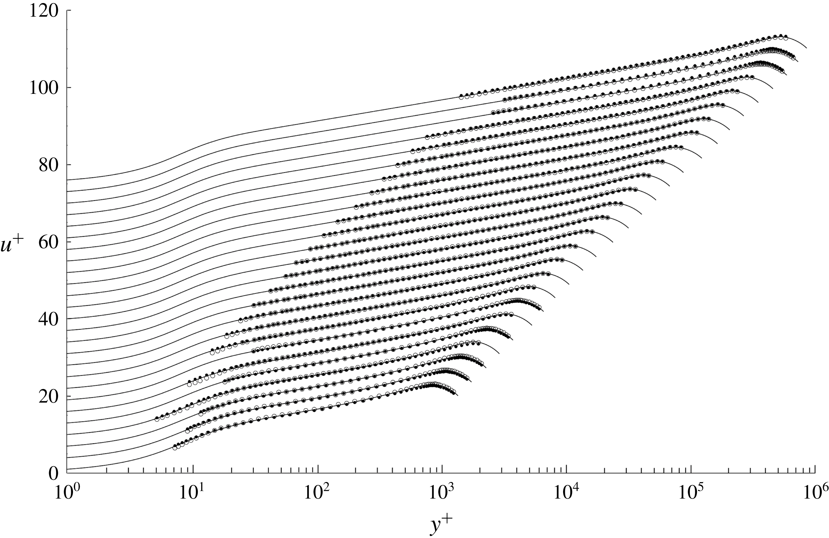


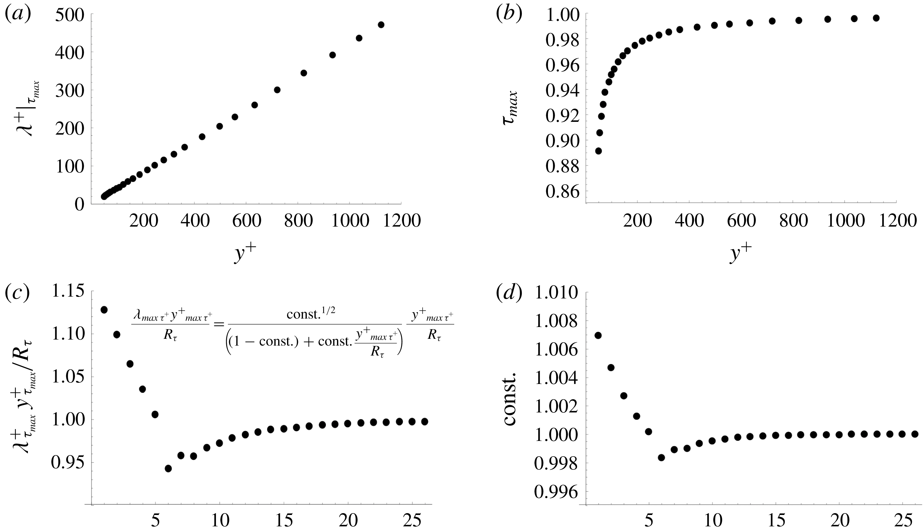


 Open access

