1 Introduction
Turbulent flows are encountered in a wide variety of fluid mechanics problems such as aerodynamic stall on airfoils (Corke & Thomas Reference Corke and Thomas2015), mixing of fluids (Dimotakis Reference Dimotakis2005) and unsteady flows in turbines (Graham Reference Graham2017), among many more. While experimental investigations have provided valuable insights into such phenomena, the attainable level of flexibility and the accessibility of flow field data of numerical simulations can be instrumental in deepening our understanding of the fundamental physics in such flows. Despite major progress in the field, predictive methods for realistic scientific and engineering applications are still the focus of current research. Moreover, fully developed turbulent flows exhibit a vast range of dynamically active scales, which need to be taken into account in order to capture all pertinent features of the flow.
Despite impressive advances over the last decades, traditional approaches to direct numerical simulation (DNS) remain prohibitively expensive from a computational standpoint, and therefore alternative methods, offering improved efficiency, are constantly sought. In this respect, the lattice Boltzmann method (LBM) (McNamara & Zanetti Reference McNamara and Zanetti1988; Higuera & Jimenez Reference Higuera and Jimenez1989; Higuera, Succi & Benzi Reference Higuera, Succi and Benzi1989; Benzi, Succi & Vergassola Reference Benzi, Succi and Vergassola1992; Chen & Doolen Reference Chen and Doolen1998; Succi Reference Succi2001, Reference Succi2015) has gained an increasingly visible role as a competitive computational fluid dynamics (CFD) tool for DNS studies. However, even with LBMs, DNS of most applications involving flows in a turbulent regime remains far beyond the current computing capabilities. For this reason, LBMs are typically supplemented with a variety of explicit turbulence models. For example, in Hou et al. (Reference Hou, Sterling, Chen and Doolen1996), Chen et al. (Reference Chen, Kandasamy, Orszag, Shock, Succi and Yakhot2003) and Malaspinas & Sagaut (Reference Malaspinas and Sagaut2012), the Bhatnagar–Gross–Krook (BGK) collision operator is augmented and a turbulent eddy viscosity is introduced by replacing the single relaxation time with a turbulent relaxation time. An exhaustive review of explicit turbulence models for LBMs can be found in Jahanshaloo et al. (Reference Jahanshaloo, Pouryazdanpanah, Azwadi and Sidik2013).
An alternative towards the simulation of turbulent flows is the crystallographic LBM (Namburi, Krithivasan & Ansumali Reference Namburi, Krithivasan and Ansumali2016), where a grid structure, based on a body-centred cubic discretization, is used to improve numerical performances. Another viable approach is the entropic lattice Boltzmann method (ELBM) (Karlin, Ferrante & Öttinger Reference Karlin, Ferrante and Öttinger1999; Boghosian et al. Reference Boghosian, Yepez, Coveney and Wagner2001; Ansumali & Karlin Reference Ansumali and Karlin2002; Karlin et al. Reference Karlin, Ansumali, Angelis, Öttinger and Succi2003) and its extension to multiple relaxation times, the so-called KBC model (Karlin, Bösch & Chikatamarla Reference Karlin, Bösch and Chikatamarla2014; Bösch, Chikatamarla & Karlin Reference Bösch, Chikatamarla and Karlin2015). KBC models have shown outstanding results for both resolved and under-resolved simulations, for a variety of fluid dynamics problems, including laminar, transitional (Dorschner, Chikatamarla & Karlin Reference Dorschner, Chikatamarla and Karlin2017b ) and fully developed turbulent flows (Dorschner et al. Reference Dorschner, Bösch, Chikatamarla, Boulouchos and Karlin2016a ,Reference Dorschner, Frapolli, Chikatamarla and Karlin b ; Dorschner, Chikatamarla & Karlin Reference Dorschner, Chikatamarla and Karlin2017a ).
Other established LBMs for turbulent flows are based on different collision models (Gehrke, Janssen & Rung Reference Gehrke, Janssen and Rung2017; Nathen et al. Reference Nathen, Gaudlitz, Krause and Adams2017). However, these methods are challenged in under-resolved simulations and need further consolidation before a judgement can be made on their competitiveness for turbulent flows.
In spite of the recent progress of LBMs for the numerical simulation of turbulent flows, a major gap remains between such an approach and traditional state-of-the-art CFD techniques, which is related to the inherent spatial discretization of LBMs on uniform Cartesian meshes. This limitation affects the range of applicability of LBMs, especially when complex geometries are involved, such as those commonly encountered in many engineering problems, where the geometric flexibility of an unstructured/non-uniform grid is required. Moreover, for turbulent flows, numerical strategies based on non-uniform stretched grids are crucial to reduce the computational costs of simulations. To address this issue many refinement approaches and body-fitted mesh schemes have been proposed.
Multidomain grid refinement techniques employ uniformly refined patches, which are embedded in those regions of the fluid domain where a higher resolution is required (Filippova & Hänel Reference Filippova and Hänel1998; Dorschner et al. Reference Dorschner, Frapolli, Chikatamarla and Karlin2016b ).
As far as unstructured grids are concerned, the first so-called off-lattice Boltzmann methods (OLBMs) are due to Peng et al. (Reference Peng, Xi, Duncan and Chou1998, Reference Peng, Xi, Duncan and Chou1999) and Xi, Peng & Chou (Reference Xi, Peng and Chou1999), who proposed finite-volume (FV) formulations of the lattice Boltzmann equation. Later, stability was enhanced by the developments of Ubertini, Bella & Succi (Reference Ubertini, Bella and Succi2003, Reference Ubertini, Bella and Succi2006), Ubertini, Succi & Bella (Reference Ubertini, Succi and Bella2004), Patil & Lakshmisha (Reference Patil and Lakshmisha2009), Zarghami et al. (Reference Zarghami, Maghrebi, Ghasemi and Ubertini2012) and Patil (Reference Patil2013). The mentioned FV schemes have led to a significant enhancement of the LBM in terms of geometrical flexibility. However, all of them are characterized by a considerably lower computational efficiency compared to traditional LBM. To cope with this drawback, a hybrid formulation which combines a traditional lattice Boltzmann approach with a FV formulation has recently been proposed by Di Ilio et al. (Reference Di Ilio, Chiappini, Ubertini, Bella and Succi2017).
Extensions of LBMs to non-uniform stretched and unstructured grids have also been proposed in Lee & Lin (Reference Lee and Lin2001, Reference Lee and Lin2003), Min & Lee (Reference Min and Lee2011) and Patel & Lee (Reference Patel and Lee2016), where Galerkin-type finite-element methods are introduced. Other OLBMs are the Discrete Unified Gas Kinetic Scheme (DUGKS) (Zhu, Wang & Guo Reference Zhu, Wang and Guo2017) and the general characteristics-based off-lattice Boltzmann scheme proposed by Bardow, Karlin & Gusev (Reference Bardow, Karlin and Gusev2006) (see, for example, Rao & Schaefer (Reference Rao and Schaefer2015) for a comparative study of several explicit OLBMs). More recently, a semi-Lagrangian approach based on the finite-element reconstruction of the distribution functions has been proposed (Krämer et al. Reference Krämer, Küllmer, Reith, Joppich and Foysi2017) and is adopted in this work.
Despite the large amount of OLBMs available, as of today, simulations of turbulent flows using OLBMs are scarce in the literature. In Amati, Succi & Benzi (Reference Amati, Succi and Benzi1997) and Li et al. (Reference Li, Zhong, Zhuo and Cao2012), numerical simulations of highly turbulent flows are performed via a non-uniform stretched non-body-fitted mesh. In Imamura et al. (Reference Imamura, Suzuki, Nakamura and Yoshida2005) and Zhuo et al. (Reference Zhuo, Zhong, Li, Xiong, Chen and Cao2010), methods are instead based on a non-uniform orthogonal conforming mesh. Another non-uniform orthogonal strategy based on Taylor series expansion and a least-squares-based lattice Boltzmann approach (TLLBM) has been investigated for turbulent flows by Shu et al. (Reference Shu, Peng, Zhou and Chew2006). Among the applications of OLBMs to turbulence, the only one to be based on an unstructured/body-fitted approach is the so-called lattice Boltzmann flux solver (LBFS) (Shu et al. Reference Shu, Wang, Teo and Wu2014), which has been adopted by Pellerin, Leclaire & Reggio (Reference Pellerin, Leclaire and Reggio2017) to simulate a turbulent flow over an airfoil. In all of the aforementioned studies, the lattice Boltzmann approach was used in conjunction with an explicit turbulence model, in two dimensions (with exception of Amati et al. (Reference Amati, Succi and Benzi1997)).
In this work, we combine the KBC model with a body-fitted mesh strategy, based on a semi-Lagrangian approach (SLLBM). The choice of employing this particular off-lattice Boltzmann scheme for the present study is driven by two reasons. First, the SLLBM exhibits a stable behaviour at relatively large Courant–Friedrichs–Lewy (CFL) numbers. This implies that the time step is mainly limited by the relevant time and length scales of the flow. This is a clear advantage over several previous unstructured lattice Boltzmann formulations. Moreover, in the SLLBM, the numerical formulation is based on a characteristic equation rather than a differential equation. This avoids problems inherent to the temporal and spatial discretization of derivatives, which are encountered when using finite-volume/finite-difference schemes. Second, as it will be detailed in the next section, the present SLLBM does not change the collision step, but rather performs the streaming step by using a high-order finite-element representation.
In conclusion, the SLLBM seems to represent a practical generalization of standard LBMs, since it effectively removes the restriction related to the regular lattice. In Krämer et al. (Reference Krämer, Küllmer, Reith, Joppich and Foysi2017), encouraging results for two- and three-dimensional cases are shown, thus projecting this method as an efficient and accurate scheme, in particular for flows requiring high spatial resolutions.
To the best of our knowledge, the SLLBM has never been applied to wall-bounded turbulence in three dimensions. Therefore, in this study we want to assess the viability of this approach for turbulence. In particular, with the aim of exploring the capabilities of the proposed method for turbulent flow simulations, we investigate the incompressible flow past a circular cylinder at Reynolds number
 $Re=3900$
and compare the results with available literature data. The remainder of the paper is organized as follows: In § 2, we describe the numerical method used in this work. In § 3, we consider the flow past a circular cylinder in the laminar regime and perform a convergence study. In § 4, we present results for the flow past a circular cylinder at
 $Re=3900$
. Finally, in § 5, a discussion of the results is provided.
2 Entropy-based semi-Lagrangian OLBM
In this study, we use a semi-Lagrangian OLBM (Krämer et al. Reference Krämer, Küllmer, Reith, Joppich and Foysi2017) combined with the KBC model (Karlin et al. Reference Karlin, Bösch and Chikatamarla2014) for the standard D3Q27 lattice. In this section, we briefly describe the main steps of the numerical approach.
2.1 KBC model
The general form of the lattice Boltzmann equation may be written as follows:
 $$\begin{eqnarray}f_{i}(\boldsymbol{x}+\boldsymbol{c}_{i}\unicode[STIX]{x1D6FF}t,t+\unicode[STIX]{x1D6FF}t)=\left(1-\unicode[STIX]{x1D6FD}\right)f_{i}(\boldsymbol{x},t)+\unicode[STIX]{x1D6FD}f_{i}^{mirr}(\boldsymbol{x},t),\end{eqnarray}$$
where
 $f_{i}$
represents the distribution function along the
 $i$
th lattice direction,
 $f_{i}^{mirr}$
is the mirror state,
 $\unicode[STIX]{x1D6FD}$
is the relaxation parameter and
 $\boldsymbol{c}_{i}$
corresponds to the following set of discrete speeds:
 $$\begin{eqnarray}\boldsymbol{c}_{i}=\left\{\begin{array}{@{}ll@{}}(0,0,0),\quad & i=1,\\ (\pm 1,0,0),(0,\pm 1,0),(0,0,\pm 1),\quad & i=2,\ldots ,7,\\ (\pm 1,\pm 1,0),(\pm 1,0,\pm 1),(0,\pm 1,\pm 1),\quad & i=8,\ldots ,19,\\ (\pm 1,\pm 1,\pm 1),\quad & i=20,\ldots ,27.\end{array}\right.\end{eqnarray}$$
With the BGK approximation, the mirror state is given by:
 $$\begin{eqnarray}f_{i}^{mirr}=2f_{i}^{eq}-f_{i},\end{eqnarray}$$
where the equilibrium distribution function is expressed as follows:
 $$\begin{eqnarray}f_{i}^{eq}\left(\boldsymbol{x},t\right)=w_{i}\unicode[STIX]{x1D70C}\left(\boldsymbol{x},t\right)\left\{1+{\displaystyle \frac{\boldsymbol{c}_{i}\cdot \boldsymbol{u}\left(\boldsymbol{x},t\right)}{c_{s}^{2}}}+{\displaystyle \frac{\left[\boldsymbol{c}_{i}\cdot \boldsymbol{u}\left(\boldsymbol{x},t\right)\right]^{2}}{2c_{s}^{4}}}-{\displaystyle \frac{\left[\boldsymbol{u}\left(\boldsymbol{x},t\right)\right]^{2}}{2c_{s}^{2}}}\right\}.\end{eqnarray}$$
In (2.4),
 $c_{s}=1/\sqrt{3}$
is the speed of sound,
 $\unicode[STIX]{x1D70C}\left(\boldsymbol{x},t\right)$
and
 $\boldsymbol{u}\left(\boldsymbol{x},t\right)$
are the fluid density and velocity, respectively, while the parameters
 $w_{i}$
are weights normalized to one, as follows:
 $$\begin{eqnarray}w_{i}=\left\{\begin{array}{@{}ll@{}}8/27,\quad & i=1,\\ 2/27,\quad & i=2,\ldots ,7,\\ 1/54,\quad & i=8,\ldots ,19,\\ 1/216,\quad & i=20,\ldots ,27.\end{array}\right.\end{eqnarray}$$
The macroscopic variables are calculated from the first two moments of the distribution functions:
 $$\begin{eqnarray}\left.\begin{array}{@{}c@{}}\displaystyle \unicode[STIX]{x1D70C}\left(\boldsymbol{x},t\right)=\mathop{\sum }_{i=1}^{Q}f_{i}\left(\boldsymbol{x},t\right),\\ \displaystyle \unicode[STIX]{x1D70C}\boldsymbol{u}\left(\boldsymbol{x},t\right)=\mathop{\sum }_{i=1}^{Q}\boldsymbol{c}_{i}f_{i}\left(\boldsymbol{x},t\right),\end{array}\right\}\end{eqnarray}$$
where
 $Q$
refers to the number of distribution functions. The lattice Boltzmann equation (2.1) recovers the Navier–Stokes (NS) equations for isothermal flow with the kinematic viscosity:
 $$\begin{eqnarray}\unicode[STIX]{x1D708}=c_{s}^{2}\left(\frac{1}{2\unicode[STIX]{x1D6FD}}-\frac{1}{2}\right)\unicode[STIX]{x1D6FF}t.\end{eqnarray}$$
For the KBC model, the populations
 $f_{i}$
are described in terms of moments as:
 $$\begin{eqnarray}f_{i}=k_{i}+s_{i}+h_{i},\end{eqnarray}$$
where
 $k_{i}$
corresponds to the kinematic part,
 $s_{i}$
is the shear part and
 $h_{i}$
represents the remaining higher-order moments. By adopting this decomposition, the mirror state can be described as:
 $$\begin{eqnarray}f_{i}^{mirr}=k_{i}+(2s_{i}^{eq}-s_{i})+[(1-\unicode[STIX]{x1D6FE})h_{i}+\unicode[STIX]{x1D6FE}h_{i}^{eq}],\end{eqnarray}$$
where
 $s_{i}^{eq}$
and
 $h_{i}^{eq}$
are the shear and the higher-order moments at equilibrium, respectively, while the parameter
 $\unicode[STIX]{x1D6FE}$
represents the relaxation of the higher-order moments. We shall notice that for the case of
 $\unicode[STIX]{x1D6FE}=2$
, the lattice BGK model is recovered. In contrast, in the KBC model, the relaxation parameter
 $\unicode[STIX]{x1D6FE}$
is found by minimizing the discrete H-function in the post-collision state. This yields the following expression:
 $$\begin{eqnarray}\unicode[STIX]{x1D6FE}=\frac{1}{\unicode[STIX]{x1D6FD}}-\left(2-\frac{1}{\unicode[STIX]{x1D6FD}}\right)\frac{\langle \unicode[STIX]{x0394}s\mid \unicode[STIX]{x0394}h\rangle }{\langle \unicode[STIX]{x0394}h\mid \unicode[STIX]{x0394}h\rangle },\end{eqnarray}$$
where the entropic scalar product is defined as:
 $$\begin{eqnarray}\langle X\mid Y\rangle =\mathop{\sum }_{i=1}^{Q}\frac{X_{i}Y_{i}}{f_{i}^{eq}},\end{eqnarray}$$
with
 $\unicode[STIX]{x0394}s_{i}=s_{i}-s_{i}^{eq}$
and
 $\unicode[STIX]{x0394}h_{i}=h_{i}-h_{i}^{eq}$
.
For the KBC realization used in this work, the populations
 $f_{i}$
have been represented in terms of their natural moments, and the shear part
 $s_{i}$
includes only the deviatoric stress tensor.
2.2 Semi-Lagrangian method
The semi-Lagrangian OLBM consists of obtaining the solution of the lattice Boltzmann equation (2.1) at the departure points of the characteristic lines via finite-element-based interpolation. Within this framework, the streaming step is realized by means of a semi-Lagrangian procedure, while the collision step remains local as in classical LBM.
In order to solve the semi-Lagrangian advection, we need to reconstruct the distribution function
 $f_{i}$
at the departure location
 $\boldsymbol{x}-\unicode[STIX]{x1D6FF}t\boldsymbol{c}_{i}$
. In the limiting case of a regular Cartesian grid with spacing
 $\unicode[STIX]{x1D6FF}t\boldsymbol{c}_{i}$
, departure points are also grid nodes, and therefore the SLLBM recovers the classical LBM. For unstructured meshes, this is not necessarily the case and an accurate reconstruction is crucial. This situation is depicted in figure 1.
Schematic of the semi-Lagrangian streaming step of population
 $f_{i}(\boldsymbol{x},t)$
along the discrete velocity
 $\boldsymbol{c}_{i}$
. The values of the distribution function at the departure point (red open circle) is obtained by means of a finite-element-based interpolation scheme involving the values of the distribution function at support points (red filled circles).

In this work, the computational domain is discretized into an irregular mesh, which is composed of
 $N_{\unicode[STIX]{x1D709}}$
hexahedral elements. The finite-element interpolation scheme is based on a set of
 $k$
th-order shape functions, which are defined on
 $N_{p}=(k+1)^{D}$
support points. In particular, we use a quadratic finite element with second-order Lagrange polynomials defined on 27 equidistant support points. A bijective multilinear transformation is used to map the reference unit cell into the physical elements of the mesh. By representing the distribution functions via a finite element instead of a point-wise approximation, we can write:
 $$\begin{eqnarray}f_{i}(\boldsymbol{x},t)=\mathop{\sum }_{\unicode[STIX]{x1D709}=1}^{N_{\unicode[STIX]{x1D709}}}\mathop{\sum }_{p=1}^{N_{p}}f_{i\unicode[STIX]{x1D709}p}(t)\unicode[STIX]{x1D713}_{\unicode[STIX]{x1D709}p}(\boldsymbol{x}),\end{eqnarray}$$
where
 $f_{i\unicode[STIX]{x1D709}p}(t)$
and
 $\unicode[STIX]{x1D713}_{\unicode[STIX]{x1D709}p}(\boldsymbol{x})$
denote the populations and shape function values at the support points for each cell, respectively. In order to approximate the distribution function at each support point, we reconstruct populations at departure points by applying (2.12). Thus, the semi-Lagrangian streaming step reads as follows:
 $$\begin{eqnarray}f_{i\unicode[STIX]{x1D709}p}(t)=f_{i}(\boldsymbol{x}_{\unicode[STIX]{x1D709}p}-\unicode[STIX]{x1D6FF}t\boldsymbol{c}_{i},t-\unicode[STIX]{x1D6FF}t)=\mathop{\sum }_{\unicode[STIX]{x1D701}=1}^{N_{\unicode[STIX]{x1D709}}}\mathop{\sum }_{q=1}^{N_{p}}f_{i\unicode[STIX]{x1D701}q}(t-\unicode[STIX]{x1D6FF}t)\unicode[STIX]{x1D713}_{\unicode[STIX]{x1D701}q}(\boldsymbol{x}_{\unicode[STIX]{x1D709}p}-\unicode[STIX]{x1D6FF}t\boldsymbol{c}_{i}).\end{eqnarray}$$
We set the time step as
 $\unicode[STIX]{x1D6FF}t=\unicode[STIX]{x1D6FF}x_{min}/\sqrt{3}$
, where
 $\unicode[STIX]{x1D6FF}x_{min}$
is the minimum spacing between any two vertices of the computational mesh. The choice is motivated to ensure that each departure point remains inside the current or nearest neighbouring cell. While the SLLBM remains stable even for larger time steps (Krämer et al.
Reference Krämer, Küllmer, Reith, Joppich and Foysi2017), the limiting case of
 $\unicode[STIX]{x1D6FF}t=2\unicode[STIX]{x1D6FF}x_{min}$
and a regular Cartesian grid results in two independent solutions. Such unphysical decoupling is avoided effectively by our choice of time step.
The numerical scheme for the semi-Lagrangian advection is fully explicit, and can be formulated in terms of simple matrix–vector multiplications, yielding:
 $$\begin{eqnarray}\boldsymbol{f}_{i}(t)=\unicode[STIX]{x1D733}_{i}\boldsymbol{f}_{i}(t-\unicode[STIX]{x1D6FF}t),\end{eqnarray}$$
where
 $\unicode[STIX]{x1D733}_{i}$
is the matrix of shape functions, and
 $\boldsymbol{f}_{i}$
denotes the distribution function vector. We emphasize that each matrix
 $\unicode[STIX]{x1D733}_{i}$
is sparse and (2.14) can therefore be evaluated numerically in a very efficient way.
The SLLBM has been implemented on the basis of the finite-element library Deal.II (Bangerth, Hartmann & Kanschat Reference Bangerth, Hartmann and Kanschat2007) and Trilinos for the linear algebra (Heroux et al. Reference Heroux, Bartlett, Howle, Hoekstra, Hu, Kolda, Lehoucq, Long, Pawlowski and Phipps2005).
2.2.1 No-slip boundary condition
As far as the no-slip boundary condition is concerned, for the SLLBM it is natural to use a similar interpolation scheme as in the bulk. Therefore, we employ a modified version of the interpolated bounce-back (IBB) approach (Bouzidi, Firdaouss & Lallemand Reference Bouzidi, Firdaouss and Lallemand2001).
Schematic of the interpolated bounce-back boundary condition for the population
 $f_{i}(\boldsymbol{x}_{b},t)$
along the discrete velocity
 $\boldsymbol{c}_{i}$
.

The IBB scheme is used to approximate the missing populations at nodes for which the departure point lies outside the fluid domain. The general problem is depicted in figure 2. Using a bounce-back type boundary condition, which reflects the population at the wall boundary, we define the departure point
 $\boldsymbol{x}_{b}^{\prime }$
as follows:
 $$\begin{eqnarray}\boldsymbol{x}_{b}^{\prime }=\boldsymbol{x}_{w,i}+(\unicode[STIX]{x1D6FF}t-q_{i})\overline{\boldsymbol{c}_{i}},\end{eqnarray}$$
where
 $q_{i}$
represents the distance between the support point and the wall boundary, along the
 $i$
th direction, and
 $\boldsymbol{x}_{w,i}$
is the intersection point between the particle trajectory along the discrete velocity
 $\overline{\boldsymbol{c}_{i}}=-\boldsymbol{c}_{i}$
and the wall boundary. The coordinates of point
 $\boldsymbol{x}_{w,i}$
are given by the following:
 $$\begin{eqnarray}\boldsymbol{x}_{w,i}=\boldsymbol{x}_{b}+q_{i}\boldsymbol{c}_{i}.\end{eqnarray}$$
The application of the boundary condition at
 $\boldsymbol{x}_{b}$
then reduces to a reconstruction of the distribution function
 $\overline{f}_{i}(\boldsymbol{x}_{b}^{\prime },t-\unicode[STIX]{x1D6FF}t)$
, which is associated with the velocity
 $\overline{\boldsymbol{c}_{i}}$
. Therefore, the reconstruction of the missing population
 $f_{i}(\boldsymbol{x}_{b},t)$
at the boundary support point
 $\boldsymbol{x}_{b}$
is given by the following finite-element interpolation:
 $$\begin{eqnarray}f_{i}(\boldsymbol{x}_{b},t)=\overline{f}_{i}(\boldsymbol{x}_{b}^{\prime },t-\unicode[STIX]{x1D6FF}t)=\mathop{\sum }_{\unicode[STIX]{x1D709}=1}^{N_{\unicode[STIX]{x1D709}}}\mathop{\sum }_{p=1}^{N_{p}}\overline{f}_{i\unicode[STIX]{x1D709}p}(t-\unicode[STIX]{x1D6FF}t)\unicode[STIX]{x1D713}_{\unicode[STIX]{x1D709}p}(\boldsymbol{x}_{b}^{\prime }).\end{eqnarray}$$
3 Convergence study
To validate the SLLBM in combination with the KBC model and the interpolated bounce-back boundary condition, we perform a convergence study by simulating the three-dimensional fluid flow past a circular cylinder in the laminar regime. The Reynolds number is defined in terms of the free-stream velocity
 $u_{\infty }$
and the diameter of the cylinder
 $D$
as
 $Re=u_{\infty }D/\unicode[STIX]{x1D708}$
and set to
 $Re=40$
. In this regime, the wake behind the cylinder is characterized by the presence of a steady recirculation region.
The analysis is carried out on four meshes of different resolution and results for the pressure coefficient
 $C_{p}$
and skin-friction coefficient
 $C_{f}$
are compared with those provided by Tseng & Ferziger (Reference Tseng and Ferziger2003). These parameters are typically used to characterize the flow field and are defined as follows:
 $$\begin{eqnarray}C_{p}=\frac{p-p_{\infty }}{\frac{1}{2}\unicode[STIX]{x1D70C}_{\infty }u_{\infty }^{2}},\quad C_{f}=\frac{\unicode[STIX]{x1D70F}_{w}}{\frac{1}{2}\unicode[STIX]{x1D70C}_{\infty }u_{\infty }^{2}},\end{eqnarray}$$
where
 $\unicode[STIX]{x1D70F}_{w}$
is the local wall shear stress, while
 $p$
and
 $p_{\infty }$
are the local pressure and the pressure in the free stream.
The computational domain is given by
 $40D\times 20D\times 1D$
for the streamwise, transverse and spanwise direction, respectively. The centroid of the cylinder is placed symmetrically in the transverse direction, at
 $10D$
from the inlet section.
We impose a uniform velocity and a zero pressure gradient at the inlet, a fixed pressure value and a zero velocity gradient at the outlet, while periodic boundary conditions are imposed in the spanwise direction. The no-slip condition as described in § 2.2.1 is applied on the cylinder surface.
3.1 Results
Figure 3 shows the deviation of the computed mean pressure coefficient from the reference
 $C_{p_{ref}}$
as a function of the minimum cell spacing. We notice that the order of convergence of the present scheme is slightly greater than 2. This is in agreement with the results presented by Krämer et al. (Reference Krämer, Küllmer, Reith, Joppich and Foysi2017), whose numerical study lead to the same conclusion for fluid flows in fully periodic domains. Next, figures 4 and 5 show the distribution of the mean pressure coefficient and the mean skin-friction coefficient over the cylinder surface, as computed with the finest mesh. The results are then compared with those available from Tseng & Ferziger (Reference Tseng and Ferziger2003). The obtained results are in good agreement with the reference data and therefore validate the proposed scheme for curved geometries.
Convergence of the unstructured method with respect to the grid refinement. The numerical results are represented by open circles; the solid thick line is the fitting curve; the dashed line represents second-order convergence, while the dotted line is representative of the third-order convergence.

Mean pressure coefficient distribution from the front (
 $\unicode[STIX]{x1D711}=0^{\circ }$
) to the rear (
 $\unicode[STIX]{x1D711}=180^{\circ }$
) stagnation point of the cylinder. Open squares: present study; open circles: reference solution from Tseng & Ferziger (Reference Tseng and Ferziger2003).

Mean skin-friction coefficient distribution from the front (
 $\unicode[STIX]{x1D711}=0^{\circ }$
) to the rear (
 $\unicode[STIX]{x1D711}=180^{\circ }$
) stagnation point of the cylinder. Open squares: present study; open circles: reference solution from Tseng & Ferziger (Reference Tseng and Ferziger2003).

4 Fluid flow past a circular cylinder at
 $Re=3900$

In this section, we present a numerical investigation of the turbulent flow around a circular cylinder in the lower subcritical range at
 $Re=3900$
. In this regime, the flow separation is laminar, while transition to turbulence occurs downstream of the cylinder in the free shear layer. Along the wake, the high instability of the flow causes a periodic vortex shedding process, which in turn leads to a vertical oscillatory motion of the free shear layer.
These features make the computation of such a flow and the prediction of its unsteady dynamics an interesting as well as a particularly challenging task. Several experimental and numerical works exist in the literature and, for this reason, has become a canonical benchmark case to assess the performance and accuracy of numerical methods. Among others, the experiments of Lourenco & Shih (Reference Lourenco and Shih1993), Norberg (Reference Norberg1994) and Ong & Wallace (Reference Ong and Wallace1996) provide an exhaustive insight on the main features of the turbulent flow under consideration. As far as numerical investigations are concerned, direct simulation of all scales of such a turbulent flow results in a high computational cost. This represents a severe constraint and therefore most studies are conducted using large eddy simulations (LES). Within this framework, we mention the works of Beaudan & Moin (Reference Beaudan and Moin1994), Kravchenko & Moin (Reference Kravchenko and Moin2000), You & Moin (Reference You and Moin2006) and Rajani, Kandasamy & Majumdar (Reference Rajani, Kandasamy and Majumdar2016), which support the findings of the previous experimental studies. Few other works on the flow around circular cylinders in the lower subcritical range have been conducted with DNS such as Ma, Karamonos & Karniadakis (Reference Ma, Karamonos and Karniadakis2000), Dong et al. (Reference Dong, Karniadakis, Ekmekci and Rockwell2006), Wissink & Rodi (Reference Wissink and Rodi2008) and Rai (Reference Rai2010). All of these numerical studies have been carried out with traditional CFD approaches, which are based on Navier–Stokes equations solvers.
The motivation behind the present analysis is to assess the capabilities of the proposed unstructured LBM to capture the main physical features of a turbulent flow for a complex fluid dynamics problem involving curved geometries. In particular, to limit the computational cost of the simulation, we shall focus our attention on near-wake turbulent phenomena. Thus, by taking advantage of the implicit subgrid features of the KBC model, we construct an optimized mesh which is relatively coarse in the far-field domain, while being able to resolve the flow region in the proximity of the cylinder surface.
In the next section, we provide details for the adopted numerical set-up. Later, we present the results and compare them with those available from the literature.
4.1 Numerical set-up
The present numerical simulation is performed on a computational domain of
 $20D\times 10D\times 3D$
for the streamwise, transverse and spanwise directions, respectively. The domain size has been chosen in accordance with the ones used by other researchers (see, for example, Rajani et al. (Reference Rajani, Kandasamy and Majumdar2016) for an overview of different domain sizes and grid parameters used in the literature). The centre of the cylinder is placed at
 $5D$
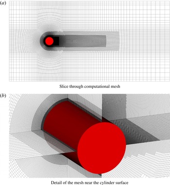
with respect to the inlet section. The computational domain is constituted of an unstructured body-fitted mesh made of hexahedral elements. The mesh is constructed to minimize the computational cost, while retaining high resolution in the close proximity of the body. In order to get accurate results, we need to resolve the near-wake region on the cylinder surface. To that end, and to further enhance the mesh efficiency, three levels of local refinements are introduced around the cylinder and along the wake region. A detail of the mesh used in this work is shown in figure 6. The adopted mesh is highly stretched, with the ratio between the largest and the smallest cell size being approximately 360. At the finest level, around the cylinder surface, the resolution in wall units, based on the maximum wall shear stress, is
 $\unicode[STIX]{x0394}\unicode[STIX]{x1D6E9}^{+}\approx 2.0$
in the circumferential direction,
 $\unicode[STIX]{x0394}r^{+}\approx 1.2$
in the radial direction and
 $\unicode[STIX]{x0394}z^{+}\approx 9.1$
in the spanwise direction, respectively. This yields a total of approximately 36 million degrees of freedom.
Unstructured mesh used for the simulation of the flow past a circular cylinder at
 $Re=3900$
. The mesh is locally refined in the proximity of the solid surface.

As far as the boundary conditions are concerned, we impose the same set as used for the convergence study in § 3. We emphasize that we use a uniform inlet velocity with no inflow disturbances. However, in order to trigger both vortex shedding and transition to turbulence, we introduce a small perturbation at the beginning of the simulation. In particular, we set the inflow velocity at
 $u_{\infty }=0.07$
in lattice units, in order to keep the Mach number at a sufficiently low value, which is
 $Ma=0.12$
, to avoid significant compressibility effects.
4.2 Results and discussion
The simulation is performed over a total time
 $t=70D/u_{\infty }$
. All statistical quantities are recorded after an initial transient of
 $t=35D/u_{\infty }$
and collected until statistically stationary conditions have been reached. Flow statistics from the current analysis are shown in this section alongside the results from previous numerical as well as experimental studies reported in the literature, for comparison.
In figures 7 and 8 we present the computed mean pressure coefficient and mean skin-friction coefficient distributions along the cylinder surface. The obtained aerodynamic coefficients distributions are compared with the numerical findings of Beaudan & Moin (Reference Beaudan and Moin1994), who used a seventh-order upwind-biased scheme for the LES of the compressible Navier–Stokes equations, and with those from the high-order accurate LES based on the B-splines of Kravchenko & Moin (Reference Kravchenko and Moin2000). Overall, our results match very well with the referred literature.
Mean pressure coefficient on the cylinder surface at
 $Re=3900$
. Open squares: present study; dotted line: LES simulation of Kravchenko & Moin (Reference Kravchenko and Moin2000); continuous line: LES simulation of Beaudan & Moin (Reference Beaudan and Moin1994).

Mean skin-friction coefficient on the cylinder surface at
 $Re=3900$
. Open squares: present study; dotted line: LES simulation of Beaudan & Moin (Reference Beaudan and Moin1994).

In particular, from figure 7, although a slight discrepancy with Kravchenko & Moin (Reference Kravchenko and Moin2000) is observed, we notice that the separation point, which can be identified as the starting point of the pressure plateau region, is properly predicted. A similar conclusion can be inferred from figure 8. The separation point corresponds to the location where the skin friction vanishes. Our prediction is in line with that of Beaudan & Moin (Reference Beaudan and Moin1994).
Streamwise velocity at three different locations, along the streamwise direction, in the wake of a circular cylinder at
 $Re=3900$
. Continuous line: present study; dotted line: LES simulation of Kravchenko & Moin (Reference Kravchenko and Moin2000); dash–dot line: DNS of Wissink & Rodi (Reference Wissink and Rodi2008) at
 $Re=3300$
; open squares: experiments of Lourenco & Shih (Reference Lourenco and Shih1993).

Vertical velocity at three different locations, along the streamwise direction, in the wake of a circular cylinder at
 $Re=3900$
. Continuous line: present study; dotted line: LES simulation of Kravchenko & Moin (Reference Kravchenko and Moin2000); dash–dot line: DNS of Wissink & Rodi (Reference Wissink and Rodi2008) at
 $Re=3300$
; open squares: experiments of Lourenco & Shih (Reference Lourenco and Shih1993).

Next, we show in figures 9 and 10 the numerical computation of the mean velocity profiles, for streamwise and transverse directions at different cross sections along the wake of the cylinder. The results are validated against the experimental measurements of Lourenco & Shih (Reference Lourenco and Shih1993), the LES of Kravchenko & Moin (Reference Kravchenko and Moin2000) and the DNS of Wissink & Rodi (Reference Wissink and Rodi2008). The numerical simulation in Wissink & Rodi (Reference Wissink and Rodi2008) was conducted at a slightly different Reynolds number (
 $Re=3300$
). Their results, however, take into account an offset in the streamwise direction which allows a direct comparison with the current case. We observe that all the computed profiles are in good agreement with the reference data. In particular, our simulation predicts the mean velocity profile
 $\overline{u}_{x}/u_{\infty }$
in the near-wake region within the experimental accuracy. On the other hand, for the transverse velocity component, the general comparison between numerical methods and experiments shows some discrepancies. However, we notice that our results show an excellent match with the DNS of Wissink & Rodi (Reference Wissink and Rodi2008). This is true especially for the mean velocity profile in the streamwise direction. Beyond mean quantities, it is interesting to analyse other statistical data of the turbulent flow (Briscolini et al.
Reference Briscolini, Santangelo, Succi and Benzi1994). Thus, in figures 11 and 12 we show the time-averaged profiles of streamwise and cross-flow components of the turbulent Reynolds stresses, while in figure 13 we present the computed turbulent Reynolds shear stress. Results from our simulations are compared with those from other numerical works using LES and with experiments of Lourenco & Shih (Reference Lourenco and Shih1993). All of the reported profiles are in very good agreement with each other, with negligible differences between our results and those from the literature. In particular, we observe that the computed profiles preserve either the shape and the symmetry, thus confirming that the analysed flow statistics are well predicted by our simulation. These results indicate that the KBC model, together with the semi-Lagrangian unstructured lattice Boltzmann formulation, can be regarded as an efficient and effective alternative to traditional CFD approaches.
Streamwise velocity fluctuations at three locations in the wake of a circular cylinder at
 $Re=3900$
. Continuous line: present study; dotted line: LES of Kravchenko & Moin (Reference Kravchenko and Moin2000); dash–dot line: LES of Beaudan & Moin (Reference Beaudan and Moin1994); dashed line: LES of Rajani et al. (Reference Rajani, Kandasamy and Majumdar2016); open squares: experiments of Lourenco & Shih (Reference Lourenco and Shih1993).

Cross-flow velocity fluctuations at three locations in the wake of a circular cylinder at
 $Re=3900$
. Continuous line: present study; dash–dot line: LES of Beaudan & Moin (Reference Beaudan and Moin1994); dashed line: LES of Rajani et al. (Reference Rajani, Kandasamy and Majumdar2016); open squares: experiments of Lourenco & Shih (Reference Lourenco and Shih1993).

Reynolds shear stress at three locations in the wake of a circular cylinder at
 $Re=3900$
. Continuous line: present study; dash–dot line: LES of Beaudan & Moin (Reference Beaudan and Moin1994); dashed line: LES of Rajani et al. (Reference Rajani, Kandasamy and Majumdar2016); open squares: experiments of Lourenco & Shih (Reference Lourenco and Shih1993).

In order to further verify that the mesh resolution is suitable to accurately describe all features of the turbulent flow, we show a snapshot of the spatial distribution of the stabilizer
 $\unicode[STIX]{x1D6FE}$
in figure 14. The value of
 $\unicode[STIX]{x1D6FE}$
is directly related to the degree of under-resolution and, as already mentioned in § 2, in the limit of a fully resolved simulation its value tends to 2. From figure 14, we observe small deviations of the stabilizer from its limit value in the near-wake region. This indicates that the flow is well resolved in this region, with negligible numerical diffusion. Analogous to the multidomain refinement in Dorschner et al. (Reference Dorschner, Frapolli, Chikatamarla and Karlin2016b
), we also notice that the entropic stabilizer detects the grid level interfaces, exhibiting significant deviations in those regions.
Instantaneous snapshot of the spatial distribution of the stabilizer
 $\unicode[STIX]{x1D6FE}$
.

Finally, in order to provide a qualitative representation of the fully developed flow field, we show isosurfaces of the Q-criterion (Hunt, Wray & Moin Reference Hunt, Wray and Moin1998) coloured by the streamwise velocity in figure 15. The instantaneous snapshot is taken at
 $t=55D/u_{\infty }$
, which corresponds to statistically stationary conditions. Observing figure 15, we notice laminar separation of the fluid flow. Beyond the separation point, transition to turbulence takes place due to three-dimensional instabilities. This leads to the formation of small-scale flow structures in the wake of the cylinder.
Isosurfaces of the Q-criterion coloured by streamwise velocity.

To conclude, the results from the current analysis clearly indicate that the unstructured semi-Lagrangian KBC model is capable of accurately predicting the main turbulent flow features and captures all relevant statistical quantities.
The proposed method presents some promising features, when compared to traditional CFD techniques. First, the current second-order unstructured lattice Boltzmann formulation has shown to provide accurate results, which are comparable to those obtained via high-order schemes for NS-based solvers. It is known that high-order methods may become unstable whenever high-gradient regions occur within the numerical solution of the fluid flow (Orszag Reference Orszag1971; Rogallo & Moin Reference Rogallo and Moin1984). This represents a major drawback for finite-difference and finite-volume NS approaches, when high accuracy is required for the numerical solution of turbulent flows at high Reynolds numbers. In these cases, the design of a stable high-order numerical method is often a complex task. In contrast, the present KBC implementation on body-fitted meshes seems to overcome this issue, since it retains the simplicity of a second-order scheme, while being stable at high Reynolds numbers. In fact, we remark that the stability properties of the KBC model are drastically enhanced compared to traditional LBMs based on the BGK approximation, for which the simulation of high-Reynolds-number flows is often not feasible.
The unstructured formulation presents advantages also with respect to traditional LBM based on uniform Cartesian mesh. The geometrical flexibility of a body-fitted mesh allows a precise definition of the solid-body surface, which can be instrumental to the solution of problems characterized by complex geometries. In addition, it allows for an extremely efficient refinement, since in the framework of the SLLBM, no particular treatment is needed to include hanging nodes. These aspects are crucial for the simulation of turbulent flows, where unstructured, stretched and locally refined meshes can significantly reduce the computational costs.
On the other hand, the semi-Lagrangian approach is limited by two main issues, which need to be addressed in future works. First, despite the presence of mesh elements of different sizes, the time step is constant in the entire computational domain, which negatively affects the overall performance. This in contrast to multidomain refinement techniques for LBMs. However, it needs to be noted that this is a peculiarity of all unstructured/non-uniform mesh approaches in the realm of LBMs. Second, the SLLBM requires a large amount of computational memory. In fact, in order to efficiently perform the streaming step, a sparse matrix needs to be stored for each population. This amounts to 27 matrices in three dimensions using the standard D3Q27 lattice. This severely limits the attainable number of degrees of freedom and thus Reynolds number for a given amount of computational resources.
A possible solution to both of these issues may be to adopt a hybrid strategy such as the one proposed in Di Ilio et al. (Reference Di Ilio, Chiappini, Ubertini, Bella and Succi2017, Reference Di Ilio, Chiappini, Ubertini, Bella and Succi2018), where the standard Cartesian LBM, possibly block-refined, is combined with an OLBM. This would allow using multidomain refinement in the far field (based on traditional LBM), while retaining an unstructured/non-uniform mesh only in the close proximity of the solid body.
5 Conclusions
In this work, we presented a numerical investigation of an unstructured lattice Boltzmann formulation based on the semi-Lagrangian streaming step together with the KBC collision model for the simulation of turbulent flows. The analysis was conducted through the simulation of the fluid flow past a circular cylinder in the lower subcritical range.
The relevant features of the flow are properly predicted by the proposed method. In particular, mean pressure and skin-friction coefficients were found to be in excellent agreement with data available from the literature. In addition, the mean velocity profiles in the vicinity of the cylinder agree well with those from previous experiments as well as from other numerical methods such as DNS and LES as used in traditional CFD approaches. Good results were also obtained in terms of time-averaged profiles for normal and shear components of the turbulent Reynolds stress tensor, which are in line with those from either numerical and experimental reference works.
These promising results open interesting prospects towards the numerical solution of turbulent flows with body-fitted meshes in the realm of LBM. The main advantages brought by the proposed method concerns the possibility of adopting a very efficient local refinement strategy. Moreover, the absence of an explicit turbulence model and the stable behaviour of the KCB model make this method a possible candidate for applications of engineering interest involving turbulent flows and a viable alternative to traditional CFD schemes based on DNS and LES.
By overcoming the uniform space discretization and the instability issues of traditional LBM based on the BGK approximation, the proposed method is likely to prove fruitful in many interdisciplinary fields. While the KBC methodology on structured grids with block refinement has shown good results in areas such transitional flows, moving geometries or thermal convection (Dorschner et al. Reference Dorschner, Frapolli, Chikatamarla and Karlin2016b , Reference Dorschner, Chikatamarla and Karlin2017a ,Reference Dorschner, Chikatamarla and Karlin b ), its extension to body-fitted meshes will significantly increase its scope in terms of attainable Reynolds number, Rayleigh number or level of complexity. For instance, it can be regarded as a powerful tool for both the study and engineering design of turbine blades and air flight capable machines, where phenomena such as boundary layer separation, transition to turbulence and reattachment of the turbulent boundary layer play an essential role. In addition, the ability to stretch the computational grid will be crucial for studies involving thermal convective turbulence, where it is important to resolve the boundary layer accurately. Applications of such flows are omnipresent, ranging from convective turbulence in stars, atmospheric or oceanic circulation to technical applications such as heat exchangers. Moreover, an extension of this method towards a moving mesh approach would make it suitable for the study of flows with suspended bodies, which are typical in chemical engineering, material science and biology. In fact, for these particular flows, the body-fitted mesh strategy represents a key element to properly and efficiently describe deformable moving objects within the flow.
Acknowledgements
This work was supported by the ETH-32-14-2 grant and the SNF grant 200021_172640. The computational resources at the Swiss National Super Computing Center CSCS were provided under grants s630 and s800. One of the authors (S.S.) wishes to acknowledge financial support from the European Research Council under the European Unions Horizon 2020 Framework Programme (No. FP/2014-2020)/ERC Grant Agreement No. 739964 (COPMAT). The authors gratefully acknowledge insightful discussions regarding the SLLBM with A. Krämer. One of the authors (G.D.I.) acknowledges funding from the Italian Ministry of Education, University and Research under PRIN grant no. 20154EHYW9. G.D.I. is grateful to Professor K. Boulouchos for the support of the stay at Aerothermochemistry and Combustion Systems Laboratory at ETH, during which this research was conducted. G.D.I. also gratefully acknowledges the support from the Scientific Consortium for the Industrial Research and Engineering (SCIRE) directed by G.B.