1 Introduction
Much of the transport observed in tokamaks, particularly in the plasma core, is believed to be caused by turbulence excited by ion-temperature-gradient (ITG) and trapped-electron-mode (TEM) instabilities. Less is known about transport and turbulence in stellarators, but ITG modes appear to be important, perhaps playing a role similar to that in tokamaks (Watanabe, Sugama & Ferrando-Margalet Reference Watanabe, Sugama and Ferrando-Margalet2008). However, there are interesting and important differences between these modes in tokamaks and stellarators. For instance, the unfavourable field-line curvature driving the ‘toroidal’ branch of the instability is often locally much larger in stellarators than in tokamaks (Helander et al. Reference Helander, Bird, Jenko, Kleiber, Plunk, Proll, Riemann and Xanthopoulos2015), but it is very unevenly distributed over the magnetic surfaces, which has a stabilising influence (Xanthopoulos et al. Reference Xanthopoulos, Plunk, Zocco and Helander2016). On the whole, though, it appears that the net transport caused by ITG modes can be comparable in tokamaks and stellarators.
The situation is very different for TEMs, which can be shown to be absent in large parts of parameter space for certain types of stellarators. The collisionless TEM is driven by trapped electrons residing in regions of bad magnetic curvature, but in so-called ‘maximum-
 $J$
’ devices (Rosenbluth Reference Rosenbluth1968) all trapped particles experience the stabilising effect of ‘good’ curvature on a time average over the orbit. For this reason, there are no collisionless, density-gradient TEMs in such configurations (Proll et al.
Reference Proll, Helander, Connor and Plunk2012; Helander, Proll & Plunk Reference Helander, Proll and Plunk2013). High-beta, quasi-isodynamic stellarators (Helander & Nührenberg Reference Helander and Nührenberg2009; Nührenberg Reference Nührenberg2010) are, to a good approximation, maximum-
 $J$
devices, and gyrokinetic simulations indeed fail to find TEMs there (Proll, Xanthopoulos & Helander Reference Proll, Xanthopoulos and Helander2013). Such modes are present in other types of stellarators, such as the Large Helical Device (Nakata et al.
Reference Nakata, Nunami, Sugama and Watanabe2016), but appear to be practically absent in Wendelstein 7-X, at least in the simulations published so far.
Instead, the simulations reveal the presence of another density-gradient-driven instability, which, in the words of Proll et al. (Reference Proll, Xanthopoulos and Helander2013), ‘evades standard classification’. The mode amplitude peaks in magnetic wells, as expected for TEMs, but the instability propagates in the ion diamagnetic direction and draws its energy from the ions rather than the electrons. It is, however, not a traditional trapped-ion mode, because the wavelength is comparable to the ion gyroradius. It is the purpose of the present paper to identify and understand the origin of this instability, which we refer to as the ion-driven TEM (ITEM). Before proceeding with the main argument for why there must be such an instability, we hasten to remark that it appears to be more benign than the conventional TEM. Nonlinear simulations so far indicate that the transport is more than one order of magnitude lower than that from TEMs in tokamaks (Helander et al. Reference Helander, Bird, Jenko, Kleiber, Plunk, Proll, Riemann and Xanthopoulos2015), probably because the wavelength perpendicular to the magnetic field is relatively short and the growth rate is fairly small. The latter feature, as we will show, can be traced to favourable spatial averaging of the ion drive.
This paper is the fourth part in a series on microinstabilities in stellarators (Helander et al. Reference Helander, Proll and Plunk2013; Proll et al. Reference Proll, Xanthopoulos and Helander2013; Plunk et al. Reference Plunk, Helander, Xanthopoulos and Connor2014) and can be considered as a logical continuation of the first part.
2 Orderings and eigenvalue problem
We adopt two orderings that are conventional in the theory of drift waves (Kadomtsev & Pogutse Reference Kadomtsev, Pogutse and Leontovich1970; Helander et al.
Reference Helander, Proll and Plunk2013). First, to avoid strong Landau damping on either electrons (
 $e$
) or ions (
 $i$
), the phase velocity
 $\unicode[STIX]{x1D714}/k_{\Vert }$
along the magnetic field is taken to satisfy
 $$\begin{eqnarray}\displaystyle v_{Ti}\ll \frac{\unicode[STIX]{x1D714}}{k_{\Vert }}\ll v_{Te}, & & \displaystyle\end{eqnarray}$$
where
 $v_{Ta}=(2T_{a}/m_{a})^{1/2}$
denotes the thermal speed of species
 $a$
. Second, the magnetic drift frequency
 $\unicode[STIX]{x1D714}_{da}=\boldsymbol{k}_{\bot }\boldsymbol{\cdot }\boldsymbol{v}_{da}$
is assumed to be much smaller than the diamagnetic frequency
 $\unicode[STIX]{x1D714}_{\ast a}=(T_{a}k_{\unicode[STIX]{x1D6FC}}/e_{a})\,\text{d}\ln n_{a}/\text{d}\unicode[STIX]{x1D713}$
,
 $$\begin{eqnarray}\displaystyle \frac{\unicode[STIX]{x1D714}_{da}}{\unicode[STIX]{x1D714}_{\ast a}}\ll 1, & & \displaystyle\end{eqnarray}$$
where the wave vector perpendicular to the magnetic field
 $\boldsymbol{B}=\unicode[STIX]{x1D735}\unicode[STIX]{x1D713}\times \unicode[STIX]{x1D735}\unicode[STIX]{x1D6FC}$
has been written as
 $\boldsymbol{k}_{\bot }=k_{\unicode[STIX]{x1D713}}\unicode[STIX]{x1D735}\unicode[STIX]{x1D713}+k_{\unicode[STIX]{x1D6FC}}\unicode[STIX]{x1D735}\unicode[STIX]{x1D6FC}$
, with
 $\unicode[STIX]{x1D713}$
the toroidal magnetic flux. As we shall see shortly, the effect of these two assumptions is effectively to decouple the ITG and TEM instabilities, which can otherwise seamlessly metamorphose into one another (Kammerer, Merz & Jenko Reference Kammerer, Merz and Jenko2008).
As shown by Helander et al. (Reference Helander, Proll and Plunk2013), by using these assumptions it is possible to reduce the electrostatic, collisionless gyrokinetic system of equations to an eigenvalue problem involving an integral equation for the electrostatic potential
 $\unicode[STIX]{x1D719}(l)$
as a function of the arc length
 $l$
along the magnetic field,
 $$\begin{eqnarray}\displaystyle f(\unicode[STIX]{x1D714},l)\unicode[STIX]{x1D719}(l)=B(l)\int _{1/B_{\text{max}}}^{1/B(l)}g(\unicode[STIX]{x1D714},\unicode[STIX]{x1D706})\overline{\unicode[STIX]{x1D719}}(\unicode[STIX]{x1D706})\frac{\text{d}\unicode[STIX]{x1D706}}{\sqrt{1-\unicode[STIX]{x1D706}B}}. & & \displaystyle\end{eqnarray}$$
Here, an overbar denotes the time average over trapped-particle orbits,
 $B_{\text{max}}$
is the maximum magnetic field strength on the flux surface in question, and we have written
 $$\begin{eqnarray}\displaystyle \left.\begin{array}{@{}c@{}}\displaystyle f(\unicode[STIX]{x1D714},l)=1+\frac{T_{e}}{T_{i}}\left[1-h(\unicode[STIX]{x1D714},l)\right],\\[15.0pt] \displaystyle g(\unicode[STIX]{x1D714},\unicode[STIX]{x1D706})=\frac{1}{2}\left[1-\frac{\unicode[STIX]{x1D714}_{\ast e}}{\unicode[STIX]{x1D714}}+\frac{3\tilde{\unicode[STIX]{x1D714}}_{de}}{2\unicode[STIX]{x1D714}}\left(1-\frac{(1+\unicode[STIX]{x1D702}_{e})\unicode[STIX]{x1D714}_{\ast e}}{\unicode[STIX]{x1D714}}\right)\right],\\[15.0pt] \displaystyle h(\unicode[STIX]{x1D714},l)=\unicode[STIX]{x1D6E4}_{0}(b)\left[1-\frac{\unicode[STIX]{x1D714}_{\ast i}}{\unicode[STIX]{x1D714}}+\frac{\hat{\unicode[STIX]{x1D714}}_{di}}{\unicode[STIX]{x1D714}}-\frac{(1+\unicode[STIX]{x1D702}_{i})\unicode[STIX]{x1D714}_{\ast i}\hat{\unicode[STIX]{x1D714}}_{di}}{\unicode[STIX]{x1D714}^{2}}\right.\\[15.0pt] \displaystyle \left.+\,b\left(\frac{\unicode[STIX]{x1D702}_{i}\unicode[STIX]{x1D714}_{\ast i}}{\unicode[STIX]{x1D714}}-\frac{\hat{\unicode[STIX]{x1D714}}_{di}}{2\unicode[STIX]{x1D714}}+\left(2\unicode[STIX]{x1D702}_{i}+\frac{1}{2}\right)\frac{\unicode[STIX]{x1D714}_{\ast i}\hat{\unicode[STIX]{x1D714}}_{di}}{\unicode[STIX]{x1D714}^{2}}\right)-b^{2}\frac{\unicode[STIX]{x1D702}_{i}\unicode[STIX]{x1D714}_{\ast i}\hat{\unicode[STIX]{x1D714}}_{di}}{\unicode[STIX]{x1D714}^{2}}\right]\\[15.0pt] \displaystyle +\,b\unicode[STIX]{x1D6E4}_{1}(b)\left[-\frac{\unicode[STIX]{x1D702}_{i}\unicode[STIX]{x1D714}_{\ast i}}{\unicode[STIX]{x1D714}}+\frac{\hat{\unicode[STIX]{x1D714}}_{di}}{2\unicode[STIX]{x1D714}}\left(1-\frac{\unicode[STIX]{x1D714}_{\ast i}}{\unicode[STIX]{x1D714}}\right)-\left(\frac{3}{2}-b\right)\frac{\unicode[STIX]{x1D702}_{i}\unicode[STIX]{x1D714}_{\ast i}\hat{\unicode[STIX]{x1D714}}_{di}}{\unicode[STIX]{x1D714}^{2}}\right],\end{array}\right\} & & \displaystyle\end{eqnarray}$$
where
 $\unicode[STIX]{x1D702}_{a}=\text{d}\ln T_{a}/\text{d}\ln n$
,
 $\unicode[STIX]{x1D6E4}_{n}(b)=e^{-b}I_{n}(b)$
,
 $b=k_{\bot }^{2}m_{i}T_{i}/(eB)^{2}$
, the ion drift frequency is expressed as
 $\unicode[STIX]{x1D714}_{di}=\hat{\unicode[STIX]{x1D714}}_{di}x^{2}(1-\unicode[STIX]{x1D706}B/2)$
and the orbit-average of the electron drift frequency as
 $\overline{\unicode[STIX]{x1D714}}_{de}=\tilde{\unicode[STIX]{x1D714}}_{de}(\unicode[STIX]{x1D706})x^{2}$
, with
 $\unicode[STIX]{x1D706}=v_{\bot }^{2}/(v^{2}B)$
and
 $x=v/v_{Ta}$
.
Equation (2.3) admits two types of solutions, depending on whether
 $\unicode[STIX]{x1D719}$
vanishes at the point
 $l_{\text{max}}$
where
 $B$
achieves its maximum value,
 $B(l_{\text{max}})=B_{\text{max}}$
. At this point, there are no trapped particles, the right-hand side of (2.3) vanishes, and so, therefore, must either
 $f$
or
 $\unicode[STIX]{x1D719}$
. In the former case, the dispersion relation is
 $f(\unicode[STIX]{x1D714},l_{\text{max}})=0$
and describes an ITG mode. In the opposite case,
 $\unicode[STIX]{x1D719}$
peaks somewhere in the trapped-particle region and the mode requires trapped electrons to exist. The ordering (2.1)–(2.2) thus allows us to discriminate between ITG modes and trapped-particle modes in an unequivocal way.
3 Dispersion relation
A useful quadratic form can be obtained by multiplying (2.3) by
 $\unicode[STIX]{x1D719}^{\ast }/B$
and integrating along the entire field line (in ballooning space),
 $$\begin{eqnarray}\displaystyle S[\unicode[STIX]{x1D719},\unicode[STIX]{x1D714}]\equiv \int _{-\infty }^{\infty }f(\unicode[STIX]{x1D714},l)|\unicode[STIX]{x1D719}|^{2}\frac{\text{d}l}{B}-\int _{1/B_{\text{max}}}^{1/B_{\text{min}}}\mathop{\sum }_{j}\unicode[STIX]{x1D70F}_{j}g(\unicode[STIX]{x1D714},\unicode[STIX]{x1D706})|\overline{\unicode[STIX]{x1D719}}_{j}|^{2}\,\text{d}\unicode[STIX]{x1D706}=0, & & \displaystyle\end{eqnarray}$$
where the sum is taken over all relevant magnetic wells (indexed by
 $j$
) with magnetic field strength
 $B<1/\unicode[STIX]{x1D706}$
, and
 $$\begin{eqnarray}\displaystyle \overline{\unicode[STIX]{x1D719}}_{j}(\unicode[STIX]{x1D706})=\frac{1}{\unicode[STIX]{x1D70F}_{j}(\unicode[STIX]{x1D706})}\int \frac{\unicode[STIX]{x1D719}(l)\,\text{d}l}{\sqrt{1-\unicode[STIX]{x1D706}B(l)}} & & \displaystyle\end{eqnarray}$$
denotes the bounce average of
 $\unicode[STIX]{x1D719}$
over the
 $j$
th such well, with
 $$\begin{eqnarray}\displaystyle \unicode[STIX]{x1D70F}_{j}(\unicode[STIX]{x1D706})=\int \frac{\text{d}l}{\sqrt{1-\unicode[STIX]{x1D706}B(l)}}. & & \displaystyle\end{eqnarray}$$
Note that the integrals over
 $l$
are taken between bounce points defined by
 $\unicode[STIX]{x1D706}B=1$
. The form
 $S[\unicode[STIX]{x1D719},\unicode[STIX]{x1D714}]$
is variational in the sense that it is stationary to first order in small variations in
 $\unicode[STIX]{x1D719}$
and
 $\unicode[STIX]{x1D714}$
satisfying the integral equation (2.3) (Helander et al.
Reference Helander, Proll and Plunk2013).
Equation (3.1) is quadratic in
 $\unicode[STIX]{x1D714}$
,
 $$\begin{eqnarray}\displaystyle P\unicode[STIX]{x1D714}^{2}+Q\unicode[STIX]{x1D714}+R=0, & & \displaystyle\end{eqnarray}$$
with coefficients
 $$\begin{eqnarray}\displaystyle \left.\begin{array}{@{}c@{}}\displaystyle P=\int _{-\infty }^{\infty }\left[1+\frac{T_{e}}{T_{i}}(1-\unicode[STIX]{x1D6E4}_{0})\right]\left|\unicode[STIX]{x1D719}\right|^{2}\frac{\text{d}l}{B}-\frac{1}{2}\int _{1/B_{\text{max}}}^{1/B_{\text{min}}}\mathop{\sum }_{j}\unicode[STIX]{x1D70F}_{j}\left|\overline{\unicode[STIX]{x1D719}}_{j}\right|^{2}\,\text{d}\unicode[STIX]{x1D706},\\[15.0pt] \displaystyle Q=\frac{\unicode[STIX]{x1D714}_{\ast i}T_{e}}{T_{i}}\int _{-\infty }^{\infty }\left[\unicode[STIX]{x1D6E4}_{0}-\unicode[STIX]{x1D702}_{i}b(\unicode[STIX]{x1D6E4}_{0}-\unicode[STIX]{x1D6E4}_{1})\right]\left|\unicode[STIX]{x1D719}\right|^{2}\frac{\text{d}l}{B}+\frac{\unicode[STIX]{x1D714}_{\ast e}}{2}\int _{1/B_{\text{max}}}^{1/B_{\text{min}}}\mathop{\sum }_{j}\unicode[STIX]{x1D70F}_{j}\left|\overline{\unicode[STIX]{x1D719}}_{j}\right|^{2}\,\text{d}\unicode[STIX]{x1D706},\\[15.0pt] \displaystyle R=\frac{\unicode[STIX]{x1D714}_{\ast i}T_{e}}{T_{i}}\int _{-\infty }^{\infty }\hat{\unicode[STIX]{x1D714}}_{di}\left[\unicode[STIX]{x1D6E4}_{0}-\frac{b(\unicode[STIX]{x1D6E4}_{0}-\unicode[STIX]{x1D6E4}_{1})}{2}+\unicode[STIX]{x1D702}_{i}\unicode[STIX]{x1D6E4}_{0}(1-b)^{2}+\unicode[STIX]{x1D702}_{i}b\left(\frac{3}{2}-b\right)\unicode[STIX]{x1D6E4}_{1}\right]\left|\unicode[STIX]{x1D719}\right|^{2}\frac{\text{d}l}{B}\\[15.0pt] \displaystyle +\,\frac{3(1+\unicode[STIX]{x1D702}_{e})\unicode[STIX]{x1D714}_{\ast e}}{4}\int _{1/B_{\text{max}}}^{1/B_{\text{min}}}\mathop{\sum }_{j}\tilde{\unicode[STIX]{x1D714}}_{dej}\unicode[STIX]{x1D70F}_{j}\left|\overline{\unicode[STIX]{x1D719}}_{j}\right|^{2}\,\text{d}\unicode[STIX]{x1D706},\end{array}\right\} & & \displaystyle \nonumber\\ \displaystyle & & \displaystyle\end{eqnarray}$$
where we have neglected terms that are small in
 $\hat{\unicode[STIX]{x1D714}}_{di}/\unicode[STIX]{x1D714}_{\ast i}\ll 1$
. The coefficient
 $P$
is positive definite due to the Schwartz inequality (see Helander et al. (Reference Helander, Proll and Plunk2013), where the quantity is denoted by
 $D[\unicode[STIX]{x1D719}]$
), but
 $Q$
and
 $R$
can have either sign. Because
 $$\begin{eqnarray}\displaystyle \unicode[STIX]{x1D714}=-\frac{1}{2P}\left(Q\pm \sqrt{Q^{2}-4PR}\right), & & \displaystyle\end{eqnarray}$$
it is clear that positive
 $R$
has a destabilising effect. We note that the first term in
 $R$
is proportional to the product
 $\unicode[STIX]{x1D714}_{\ast i}\hat{\unicode[STIX]{x1D714}}_{di}$
, which represents the instability drive from ions due to magnetic curvature, and because the function
 $$\begin{eqnarray}\displaystyle \unicode[STIX]{x1D6E4}_{0}-\frac{b(\unicode[STIX]{x1D6E4}_{0}-\unicode[STIX]{x1D6E4}_{1})}{2}+\unicode[STIX]{x1D702}_{i}\unicode[STIX]{x1D6E4}_{0}(1-b)^{2}+\unicode[STIX]{x1D702}_{i}b\left(\frac{3}{2}-b\right)\unicode[STIX]{x1D6E4}_{1} & & \displaystyle\end{eqnarray}$$
is positive for all
 $b$
if
 $\unicode[STIX]{x1D702}_{i}>0$
, it follows that the ions are destabilising if
 $\unicode[STIX]{x1D714}_{\ast i}\hat{\unicode[STIX]{x1D714}}_{di}>0$
, which is the usual criterion of unfavourable magnetic curvature. The second term in
 $R$
involves the product
 $\unicode[STIX]{x1D714}_{\ast e}\tilde{\unicode[STIX]{x1D714}}_{dej}$
, which represents the corresponding drive from electrons, bounce-averaged over the
 $j$
th trapping well. In a maximum-
 $J$
device, this product is negative for all orbits, so that the bounce-averaged curvature is favourable for all trapped particles (Rosenbluth Reference Rosenbluth1968; Proll et al.
Reference Proll, Helander, Connor and Plunk2012; Helander et al.
Reference Helander, Proll and Plunk2013). There is then no instability drive from the electrons, and conventional TEMs are absent. This was shown to be the case if
 $0<\unicode[STIX]{x1D702}_{e}<2/3$
, independently of the orderings (2.1)–(2.2), by Proll et al. (Reference Proll, Helander, Connor and Plunk2012), Helander et al. (Reference Helander, Proll and Plunk2013), and we now see it to be true for any
 $\unicode[STIX]{x1D702}_{e}>0$
if these orderings hold, because the electron contribution to
 $R$
is stabilising if
 $\unicode[STIX]{x1D714}_{\ast e}\tilde{\unicode[STIX]{x1D714}}_{dej}$
is negative. Furthermore, one can argue that positive
 $\unicode[STIX]{x1D702}_{e}$
is desirable in this case, because it amplifies a term that is already stabilising, making its effect even stronger.
Any instability must then be driven by the ions, but only arises if the stabilising influence of the term
 $Q^{2}$
in (3.6) is small enough. According to the ordering (2.2),
 $Q^{2}$
is larger than
 $PR$
, but as noticed by Coppi & Pegoraro (Reference Coppi and Pegoraro1977),
 $Q$
must go through zero as the perpendicular wavenumber is varied, due to the behaviour of the function
 $$\begin{eqnarray}\displaystyle F(b,\unicode[STIX]{x1D702}_{i})=\unicode[STIX]{x1D6E4}_{0}-\unicode[STIX]{x1D702}_{i}b(\unicode[STIX]{x1D6E4}_{0}-\unicode[STIX]{x1D6E4}_{1}), & & \displaystyle\end{eqnarray}$$
contained in the first term. To demonstrate this, let us fix our sign conventions so that
 $\unicode[STIX]{x1D714}_{\ast e}$
is negative. We observe
 $F$
tends to
 $1$
at small
 $b$
, and the first term of
 $Q$
is thus positive and larger than the second term (again using the Schwartz inequality), making
 $Q$
positive when
 $b\rightarrow 0$
. However, if
 $\unicode[STIX]{x1D702}_{i}>1.64$
,
 $F$
must become negative for
 $b$
greater than some value, a constant that we denote
 $b_{c}$
(Helander et al.
Reference Helander, Proll and Plunk2013). Therefore, the integral quantity
 $Q$
can be made negative by choosing wavenumbers
 $k_{\unicode[STIX]{x1D713}}$
and
 $k_{\unicode[STIX]{x1D6FC}}$
such that
 $b(l)>b_{c}$
for all
 $l$
, and so there must be a choice of wavenumbers where
 $Q=0$
; note that the latter choice of wavenumbers will generally be different than the former. Alternatively, if
 $\unicode[STIX]{x1D702}_{i}<1.64$
, we note that for
 $b\rightarrow \infty$
,
 $$\begin{eqnarray}\displaystyle & \displaystyle \unicode[STIX]{x1D6E4}_{0}(b)\sim \frac{1}{\sqrt{2\unicode[STIX]{x03C0}b}}\left(1+\frac{1}{8b}\right), & \displaystyle\end{eqnarray}$$
 $$\begin{eqnarray}\displaystyle & \displaystyle \unicode[STIX]{x1D6E4}_{1}(b)\sim \frac{1}{\sqrt{2\unicode[STIX]{x03C0}b}}\left(1-\frac{3}{8b}\right), & \displaystyle\end{eqnarray}$$
and the first term in
 $Q$
, although positive, becomes small. Unless
 $|\overline{\unicode[STIX]{x1D719}}_{j}|\rightarrow 0$
,
 $Q$
will therefore again pass through zero, this time at some value of
 $b$
of order the inverse of the trapped-particle fraction squared, which is formally a number of order unity in our treatment. For any
 $\unicode[STIX]{x1D702}_{i}>0$
we thus expect there to be a range of wavenumbers with
 $b=O(1)$
in which
 $Q^{2}<4PR$
and instability thus prevails. In a maximum-
 $J$
configuration, this instability is entirely driven by ions residing in regions of bad curvature, but it requires the existence of trapped electrons. The real frequency of the mode is given by
 $\unicode[STIX]{x1D714}_{r}=-Q/(2P)$
, but is limited in size by the condition on
 $Q^{2}$
. The mode will thus propagate with a frequency of order
 $(\unicode[STIX]{x1D714}_{\ast }\unicode[STIX]{x1D714}_{d})^{1/2}$
in either the ion or electron direction, with the direction changing sign at the value of
 $k_{\unicode[STIX]{x1D6FC}}$
where
 $Q$
becomes zero.
4 Iterative solution of the eigenvalue problem
In the previous section, we have demonstrated why the ITEM can exist even when the magnetic drift of trapped electrons is stabilising. However, several important questions remain. Under what conditions (e.g. in what magnetic geometries) will this mode be found? How large will its growth rate be? We have seen that the classical TEM is stable in special (maximum-
 $J$
) configurations – is it possible to devise configurations that are also immune to the ion-driven mode?
We return to the analysis of (2.3) which can be simplified by further exploiting our ordering assumptions. We have already noted that a near cancellation of the integral quantity
 $Q$
is necessary for instability. Likewise, it is necessary that the terms proportional to
 $\unicode[STIX]{x1D714}_{\ast }$
, being formally large, must independently balance in the integral equation (2.3). Thus we can solve the integral equation iteratively. At dominant order, we have
 $$\begin{eqnarray}\displaystyle \unicode[STIX]{x1D705}(l)\unicode[STIX]{x1D719}(l)=B(l)\int _{1/B_{\text{max}}}^{1/B(l)}\overline{\unicode[STIX]{x1D719}}(\unicode[STIX]{x1D706})\frac{\text{d}\unicode[STIX]{x1D706}}{\sqrt{1-\unicode[STIX]{x1D706}B}}, & & \displaystyle\end{eqnarray}$$
where the ratio of the zeroth-order parts of
 $f$
and
 $g$
is denoted by
 $\unicode[STIX]{x1D705}(l)$
. At next order we can obtain a dispersion relation for the mode frequency
 $$\begin{eqnarray}\displaystyle \int _{-\infty }^{\infty }f_{1}(\unicode[STIX]{x1D714},l)|\unicode[STIX]{x1D719}|^{2}\frac{\text{d}l}{B}=\int _{1/B_{\text{max}}}^{1/B_{\text{min}}}\mathop{\sum }_{j}g_{1}(\unicode[STIX]{x1D714},\unicode[STIX]{x1D706})\unicode[STIX]{x1D70F}_{j}\left|\overline{\unicode[STIX]{x1D719}}_{j}\right|^{2}\,\text{d}\unicode[STIX]{x1D706} & & \displaystyle\end{eqnarray}$$
where we have expressed the next-order parts of
 $f$
and
 $g$
as
 $f_{1}$
and
 $g_{1}$
. These quantities include the drive terms (proportional to
 $\unicode[STIX]{x1D714}_{d}\unicode[STIX]{x1D714}_{\ast }$
) and contributions proportional to
 $\unicode[STIX]{x1D714}_{\ast }/\unicode[STIX]{x1D714}$
, which are necessary for a non-zero real part of
 $\unicode[STIX]{x1D714}$
. The latter contributions arise mathematically by expanding
 $k_{\unicode[STIX]{x1D6FC}}=k_{\unicode[STIX]{x1D6FC}0}+k_{\unicode[STIX]{x1D6FC}1}$
, and
 $k_{\unicode[STIX]{x1D713}}=k_{\unicode[STIX]{x1D713}0}+k_{\unicode[STIX]{x1D713}1}$
. Thus,
 $\unicode[STIX]{x1D705}(l)$
is equal to the quantity
 $2F(b_{0}(l),\unicode[STIX]{x1D702}_{i})$
, where
 $F$
is defined in (3.8), and
 $b_{0}=|k_{\unicode[STIX]{x1D713}0}\unicode[STIX]{x1D735}\unicode[STIX]{x1D713}+k_{\unicode[STIX]{x1D6FC}0}\unicode[STIX]{x1D735}\unicode[STIX]{x1D6FC}|^{2}m_{i}T_{i}/(eB)^{2}$
. The quantities
 $f_{1}$
and
 $g_{1}$
include those terms proportional to
 $k_{\unicode[STIX]{x1D6FC}1}$
or
 $k_{\unicode[STIX]{x1D713}1}$
arising from the factors of
 $\unicode[STIX]{x1D714}_{\ast }/\unicode[STIX]{x1D714}$
contained in
 $f$
and
 $g$
. Explicit expressions for
 $f_{1}$
and
 $g_{1}$
are given in appendix A.
Equation (4.1) simplifies the problem, because the eigenfunction can now be determined independently of the mode frequency, and, more importantly, we observe that it cannot depend on how the ion drift
 $\hat{\unicode[STIX]{x1D714}}_{di}$
varies with
 $l$
. Therefore the mode structure will not necessarily peak preferentially at locations of bad curvature (as it does e.g. for the ITG mode). As is apparent from (4.2) (and from the full expression for
 $R$
) the ion drive contribution depends on an average of the ion magnetic drift, weighted by the mode amplitude
 $|\unicode[STIX]{x1D719}|^{2}$
, and an additional factor depending on
 $b(l)$
. We surmise, therefore, that when there are areas of both good and bad curvature within a well (which is generally the case) there will be some cancellation due to this average, helping to stabilise the mode. Furthermore, it is apparent that the ion drive can be eliminated if regions of good curvature outweigh the regions of bad curvature under this average. It is therefore of primary importance to understand this equation and its solutions.
Let us discuss the general properties of (4.1). The integral operator on the right-hand side is Hermitian. As mentioned before, the function produced by this operator must have nodes at well endpoints where
 $B=B_{\text{max}}$
. We also notice that the derivative of this function must be zero there too, because
 $B(l)$
has its maximum there. We can make a further general observation about the symmetry of solutions to (4.1). Let us assume that the magnetic well is symmetric about its centre. Then, all odd functions are in the null space of the integral operator on the right-hand side, and so the right-hand side must be an even function, which we may divide by
 $\unicode[STIX]{x1D705}(l)$
to obtain
 $\unicode[STIX]{x1D719}(l)$
. We can conclude that the asymmetry of the mode in this case is induced purely by the function
 $\unicode[STIX]{x1D705}(l)$
, which could be controlled, to some extent, by choice of magnetic geometry.
Lastly, we note that (4.1) suggests an interesting fundamental difference between tokamaks and stellarators. This difference originates from the fact that ions are assumed stationary along the field line, and only the trapped part of the electron population contributes. It is therefore only through these electrons that different points along the field line communicate, so there is no mechanism to causally connect distinct wells of height equal to the maximum
 $B_{\text{max}}$
. In tokamaks, the well structure exactly repeats along the field line, whereas in a realistic stellarator there will be a unique value of
 $B_{\text{max}}$
along the field line. Thus the entire surface of the stellarator is causally connected by a finite population of trapped electrons. Practically speaking, the numerical solution of the mode structure in a stellarator (which must be performed over a finite domain) can have a unique primary magnetic well, across which the global mode forms, coupled by trapped electrons. However, in a tokamak, there will be a number of equivalent wells (corresponding to the number of poloidal turns spanned by the simulation domain) that are decoupled, making the notion of a single ‘global mode’ somewhat artificial in this context. This suggests that it would be sensible to limit the domain in a tokamak to a single poloidal turn for the purposes of linear TEM simulations, whereas the domain length should be longer in stellarator simulations.
4.1 Square magnetic well
Despite its simplicity, (4.1) does not seem to generally admit analytical solutions. However, there is a particularly simple limit in which a solution is readily found. This is the case of a square magnetic well, i.e. a well of width
 $L$
in which the magnetic field has a constant value
 $B_{0}$
, and rises abruptly to the maximum value
 $B_{\text{max}}$
at the edges. All trapped electrons in this well have the same bounce points (at
 $l=\pm L/2$
), and the bounce average is just an
 $l$
-average over the well. We will assume
 $\unicode[STIX]{x1D702}_{i}=\unicode[STIX]{x1D702}_{e}=0$
for simplicity (this has the added benefit of ensuring that
 $\unicode[STIX]{x1D705}$
has no zeros).
From (4.1) we have
 $$\begin{eqnarray}\displaystyle \unicode[STIX]{x1D705}\unicode[STIX]{x1D719}(l)=\frac{2f_{t}}{L}\int \,\text{d}l^{\prime }\unicode[STIX]{x1D719}(l^{\prime }), & & \displaystyle\end{eqnarray}$$
where here
 $\unicode[STIX]{x1D705}=2\unicode[STIX]{x1D6E4}_{0}(b_{0})$
and we introduce the trapped-particle fraction (a constant in this case),
 $$\begin{eqnarray}\displaystyle f_{t}=\sqrt{1-\frac{B_{0}}{B_{\text{max}}}}. & & \displaystyle\end{eqnarray}$$
The function
 $\unicode[STIX]{x1D719}(l)$
is obtained by simply dividing (4.3) by
 $\unicode[STIX]{x1D705}(l)$
. We thus observe that the mode structure simply goes as
 $\unicode[STIX]{x1D705}^{-1}$
, and so it is purely determined by the spatial variation of
 $k_{\bot }$
. A further condition is then obtained by averaging
 $\unicode[STIX]{x1D719}(l)$
,
 $$\begin{eqnarray}\displaystyle \frac{1}{L}\int \frac{\text{d}l}{\unicode[STIX]{x1D705}(l)}=\frac{1}{2f_{t}}. & & \displaystyle\end{eqnarray}$$
This condition determines allowable values of
 $k_{\unicode[STIX]{x1D6FC}0}$
and
 $k_{\unicode[STIX]{x1D713}0}$
. For simplicity, we take
 $k_{\unicode[STIX]{x1D6FC}1}=0$
, and from (4.2) we obtain a dispersion relation for a purely growing (or decaying) mode
 $$\begin{eqnarray}\displaystyle \frac{4f_{t}^{2}}{L}\int \frac{\text{d}l}{\unicode[STIX]{x1D705}^{2}}\left[1+\frac{T_{e}}{T_{i}}(1-h_{1})\right]=B_{0}\int _{1/B_{\text{max}}}^{1/B_{0}}\frac{g_{1}\,\text{d}\unicode[STIX]{x1D706}}{\sqrt{1-\unicode[STIX]{x1D706}B_{0}}} & & \displaystyle\end{eqnarray}$$
where
 $$\begin{eqnarray}\displaystyle g_{1}(\unicode[STIX]{x1D714},\unicode[STIX]{x1D706})=\frac{1}{2}\left[1-\frac{3\unicode[STIX]{x1D714}_{\ast e}\tilde{\unicode[STIX]{x1D714}}_{de}}{2\unicode[STIX]{x1D714}^{2}}\right], & & \displaystyle\end{eqnarray}$$
and
 $$\begin{eqnarray}\displaystyle h_{1}(\unicode[STIX]{x1D714},l)=\unicode[STIX]{x1D6E4}_{0}(b)+\left(\frac{\unicode[STIX]{x1D714}_{\ast i}\hat{\unicode[STIX]{x1D714}}_{di}}{\unicode[STIX]{x1D714}^{2}}\right)\left[\unicode[STIX]{x1D6E4}_{0}(b)\left(\frac{b}{2}-1\right)-\frac{b}{2}\unicode[STIX]{x1D6E4}_{1}(b)\right]. & & \displaystyle\end{eqnarray}$$
Note that (4.6) is quadratic in
 $\unicode[STIX]{x1D714}$
, with no linear term, and thus it follows that, assuming electrons are stabilising (
 $\unicode[STIX]{x1D714}_{\ast e}\tilde{\unicode[STIX]{x1D714}}_{de}<0$
), instability requires that the condition
 $$\begin{eqnarray}\displaystyle \frac{1}{L}\int \frac{\text{d}l\unicode[STIX]{x1D714}_{\ast i}\hat{\unicode[STIX]{x1D714}}_{di}}{\unicode[STIX]{x1D705}^{2}}\left[\unicode[STIX]{x1D6E4}_{0}(b)\left(1-\frac{b}{2}\right)+\frac{b}{2}\unicode[STIX]{x1D6E4}_{1}(b)\right]>0, & & \displaystyle\end{eqnarray}$$
be satisfied. Note that the quantity within the brackets is positive definite, and so instability requires a kind of ‘average-bad’ curvature, where the weight of the average depends on
 $l$
only via
 $b(l)$
. As a further simplification, we can consider a system with linear magnetic shear, such that
 $\unicode[STIX]{x1D735}\unicode[STIX]{x1D6FC}=(\hat{\boldsymbol{y}}+\hat{\boldsymbol{x}}sl)|\unicode[STIX]{x1D735}\unicode[STIX]{x1D6FC}|_{l=0}$
,
 $\unicode[STIX]{x1D735}\unicode[STIX]{x1D713}=\hat{\boldsymbol{x}}|\unicode[STIX]{x1D735}\unicode[STIX]{x1D713}|_{l=0}$
, where we have introduced
 $s$
, the inverse magnetic shear length. Defining
 $k_{x}=k_{\unicode[STIX]{x1D713}}|\unicode[STIX]{x1D735}\unicode[STIX]{x1D713}|_{l=0}$
,
 $k_{y}=k_{\unicode[STIX]{x1D6FC}}|\unicode[STIX]{x1D735}\unicode[STIX]{x1D713}|_{l=0}$
, and
 $l_{0}=-k_{x}/(k_{y}s)$
, we obtain
 $k_{\bot }^{2}=k_{y}^{2}(s^{2}(l-l_{0})^{2}+1)$
. Assuming that the location
 $l_{0}$
is outside the magnetic well, at a sufficient distance, and that
 $s$
and
 $k_{y}$
are positive, we obtain
 $k_{\bot }\approx k_{y}|l-l_{0}|s$
. Then, taking
 $b\gg 1$
, we can use the large-argument expansions of
 $\unicode[STIX]{x1D6E4}_{0}$
and
 $\unicode[STIX]{x1D6E4}_{0}$
to obtain
 $$\begin{eqnarray}\displaystyle \frac{1}{\unicode[STIX]{x1D705}^{2}}\left[\unicode[STIX]{x1D6E4}_{0}(b)\left(1-\frac{b}{2}\right)+\frac{b}{2}\unicode[STIX]{x1D6E4}_{1}(b)\right]\approx \frac{3}{8}\sqrt{\frac{\unicode[STIX]{x03C0}}{2}}k_{y0}\unicode[STIX]{x1D70C}|l-l_{0}|s, & & \displaystyle\end{eqnarray}$$
Expanding (4.5) for
 $b\gg 1$
yields the solution for
 $k_{y0}$
,
 $$\begin{eqnarray}\displaystyle k_{y0}\unicode[STIX]{x1D70C}=\frac{1}{\sqrt{2\unicode[STIX]{x03C0}}|l_{0}|sf_{t}}. & & \displaystyle\end{eqnarray}$$
As a second simplification, we can take
 $\tilde{\unicode[STIX]{x1D714}}_{de}$
to be independent of pitch angle
 $\unicode[STIX]{x1D706}$
, which is a good approximation in some geometries (Kesner & Hastie Reference Kesner and Hastie2002). Then the integral on the right-hand side of (4.6) simply yields another factor of
 $2f_{t}$
. Assuming now that electrons are stabilising,
 $\unicode[STIX]{x1D714}_{\ast e}\tilde{\unicode[STIX]{x1D714}}_{de}<0$
, it is easy to devise a function
 $\unicode[STIX]{x1D714}_{di}(l)$
(involving areas of both good and bad curvature) that yields a stable mode. The strategy, which is simply to choose the values of good curvature to reside in regions that are more strongly weighted by the function
 $|l-l_{0}|$
, may not work for all values of
 $l_{0}$
, so it still seems challenging to obtain absolute stability of the ITEM mode, given that some areas of bad curvature must be present for a magnetic field line that traces out a topological torus. Still, the possibility cannot be ruled out entirely.
4.2 Numerical solutions
Let us next consider numerical solutions of (4.1). A uniform grid is used in
 $l$
-space, and the integrals in
 $l$
and
 $\unicode[STIX]{x1D706}$
are evaluated numerically. We can approach (4.1) as an eigenvalue equation, considering
 $k_{\unicode[STIX]{x1D713}}$
as a fixed parameter. We take the locations of maximum magnetic field to be
 $\pm L/2$
, normalise
 $\hat{l}=l/L$
, and decompose
 $\unicode[STIX]{x1D705}(l)=\unicode[STIX]{x1D708}_{i}\hat{\unicode[STIX]{x1D705}}(\hat{l})$
where we choose
 $\hat{\unicode[STIX]{x1D705}}(0)=1$
, and
 $\unicode[STIX]{x1D708}_{i}$
denotes the eigenvalue, with index
 $i$
. Two choices,
 $\hat{\unicode[STIX]{x1D705}}=1/|\hat{l}-1|$
, and
 $\unicode[STIX]{x1D705}=1$
are considered, corresponding, respectively, to linear magnetic shear with
 $b\gg 1$
, and zero magnetic shear. Thus, the allowable values of
 $k_{\unicode[STIX]{x1D6FC}0}$
are determined by the eigenvalues
 $\unicode[STIX]{x1D708}_{i}$
. The mode frequency
 $\unicode[STIX]{x1D714}$
can then immediately be determined by (4.2) (which is merely a quadratic dispersion relation) where
 $k_{\unicode[STIX]{x1D6FC}1}$
is a free parameter whose sign will determine the direction of mode propagation. Note that the choice
 $k_{\unicode[STIX]{x1D6FC}1}=0$
causes the quadratic form
 $Q$
to be precisely zero, and the corresponding mode must then have zero real frequency.
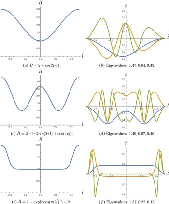
In figure 1(b), the eigenmode solutions are plotted corresponding to the sinusoidal magnetic well, figure 1(a), with
 $\hat{\unicode[STIX]{x1D705}}=1/|\hat{l}-1|$
. The resulting eigenmode asymmetry is consistent with the general arguments made above, namely that its amplitude is enhanced at negative
 $\hat{l}$
, where
 $\hat{\unicode[STIX]{x1D705}}(\hat{l})$
is smaller.
A double well structure for
 $B(l)$
, figure 1(c), results in the mode structures shown in figure 1(d). Here
 $\hat{\unicode[STIX]{x1D705}}=1$
. We can see the demonstration of other qualitative features that seem characteristic, namely the appearance of only even eigenmodes (corresponding to the non-zero eigenvalues), and eigenfunction nodes at the endpoints, where the eigenfunctions also have zero derivative.
Examples of numerical solutions of (4.1). Magnetic well plotted (
 $\hat{B}(\hat{l})=B(l)/B_{\text{min}}$
for
 $\hat{l}\in [-1/2,1/2]$
) next to first three eigenmodes (corresponding to the largest eigenvalues
 $\unicode[STIX]{x1D708}_{i}$
).

In figure 1(f), a smooth approximation to a square well, figure 1(e), has been used, demonstrating how the single mode found in the perfect square well splits into a spectrum of modes that have structure near the well endpoints, where
 $B(l)$
is non-constant (here also
 $\hat{\unicode[STIX]{x1D705}}=1$
).
5 Conclusion
In this paper, we have demonstrated the existence of an ITEM, which can exist in maximum-
 $J$
devices despite a stabilising electron magnetic drift. Although not providing free energy to the mode, trapped electrons are nevertheless required, because they reduce the phase velocity sufficiently to allow for resonance with the ion magnetic drift.
The key results are given by (3.4), (4.1) and (4.2). Several important conclusions arise from inspecting these equations. They demonstrate that the electron magnetic drift will be stabilising when the electrons are subjected to ‘good’ bounce-averaged curvature, and even more strongly stabilising with an electron temperature gradient
 $\unicode[STIX]{x1D702}_{e}>0$
. The necessary balance between the ion and trapped-electron diamagnetic drifts is a feature shared with the ‘ubiquitous mode’ of Coppi & Pegoraro (Reference Coppi and Pegoraro1977); the balance must occur at some value of
 $k_{\bot }$
, and thus this existence condition is guaranteed to be satisfied. Furthermore, we note that the case where the balance is exact will be the zero-crossing point of the real part of the mode frequency in
 $k$
-space, as is observed in numerical simulations (Proll et al.
Reference Proll, Xanthopoulos and Helander2013), where the transition occurs between ion and electron directed mode propagation.
We find that a simple integral equation, (4.1), independent of mode frequency (and independent of diamagnetic and magnetic drift frequencies) determines the mode structure (in the limit
 $\unicode[STIX]{x1D714}_{\ast }\gg \unicode[STIX]{x1D714}_{d}$
). This leads to the important conclusion that the mode structure will not necessarily peak in regions of bad curvature, and so some degree of favourable averaging should be expected to limit the overall instability of the ITEM. This could explain the relatively small growth rates that have been previously observed in numerical simulations (Proll et al.
Reference Proll, Xanthopoulos and Helander2013).
Solving (4.1) in a simple analytically tractable limit illustrates that, for certain mode wavenumbers, the ITEM may be stabilised completely by favourable averaging of the ion magnetic drift, but it is not apparent how all wavenumbers might be stabilised for realistic magnetic configurations. It is, however, noted that the mode may, for all wavenumbers, be particularly weak when the magnetic drift varies in an oscillatory manner on a scale smaller than that of the variation of
 $k_{\bot }$
. Numerical solutions of (4.1) confirm qualitative properties of the solution and demonstrate the possibility of further linear optimisation studies by numerical means.
Appendix A
Here we provide explicit expressions for the functions
 $f_{1}$
and
 $g_{1}$
:
 $$\begin{eqnarray}\displaystyle f_{1}(\unicode[STIX]{x1D714},l)=1+\frac{T_{e}}{T_{i}}\left[1-h_{1}(\unicode[STIX]{x1D714},l)\right] & & \displaystyle\end{eqnarray}$$
where
 $$\begin{eqnarray}\displaystyle h_{1}(\unicode[STIX]{x1D714},l) & = & \displaystyle \unicode[STIX]{x1D6E4}_{0}\left[1-\frac{\unicode[STIX]{x1D714}_{\ast i1}}{\unicode[STIX]{x1D714}}-\frac{(1+\unicode[STIX]{x1D702}_{i})\unicode[STIX]{x1D714}_{\ast i}\hat{\unicode[STIX]{x1D714}}_{di}}{\unicode[STIX]{x1D714}^{2}}\right.\nonumber\\ \displaystyle & & \displaystyle +\left.b_{0}\left(\frac{\unicode[STIX]{x1D702}_{i}\unicode[STIX]{x1D714}_{\ast i1}}{\unicode[STIX]{x1D714}}+\left(2\unicode[STIX]{x1D702}_{i}+\frac{1}{2}\right)\frac{\unicode[STIX]{x1D714}_{\ast i}\hat{\unicode[STIX]{x1D714}}_{di}}{\unicode[STIX]{x1D714}^{2}}\right)-b_{0}^{2}\frac{\unicode[STIX]{x1D702}_{i}\unicode[STIX]{x1D714}_{\ast i}\hat{\unicode[STIX]{x1D714}}_{di}}{\unicode[STIX]{x1D714}^{2}}\right]\nonumber\\ \displaystyle & & \displaystyle -\,b_{0}\unicode[STIX]{x1D6E4}_{1}\left[\frac{\unicode[STIX]{x1D702}_{i}\unicode[STIX]{x1D714}_{\ast i1}}{\unicode[STIX]{x1D714}}+\frac{\unicode[STIX]{x1D714}_{\ast i}\hat{\unicode[STIX]{x1D714}}_{di}}{2\unicode[STIX]{x1D714}^{2}}+\left(\frac{3}{2}-b_{0}\right)\frac{\unicode[STIX]{x1D702}_{i}\unicode[STIX]{x1D714}_{\ast i}\hat{\unicode[STIX]{x1D714}}_{di}}{\unicode[STIX]{x1D714}^{2}}\right]\nonumber\\ \displaystyle & & \displaystyle +\,b_{1}\frac{\unicode[STIX]{x1D714}_{\ast i}}{\unicode[STIX]{x1D714}}\left[(1+\unicode[STIX]{x1D702}_{i})(\unicode[STIX]{x1D6E4}_{0}-\unicode[STIX]{x1D6E4}_{1})-\frac{b_{0}\unicode[STIX]{x1D702}_{i}}{2}\left(3\unicode[STIX]{x1D6E4}_{0}-4\unicode[STIX]{x1D6E4}_{1}+\unicode[STIX]{x1D6E4}_{2}\right)\right],\end{eqnarray}$$
and
 $$\begin{eqnarray}\displaystyle g_{1}(\unicode[STIX]{x1D714},\unicode[STIX]{x1D706})=\frac{1}{2}\left[1-\frac{\unicode[STIX]{x1D714}_{\ast e1}}{\unicode[STIX]{x1D714}}-\frac{3(1+\unicode[STIX]{x1D702}_{e})\unicode[STIX]{x1D714}_{\ast e}\tilde{\unicode[STIX]{x1D714}}_{de}}{2\unicode[STIX]{x1D714}^{2}}\right], & & \displaystyle\end{eqnarray}$$
where
 $\unicode[STIX]{x1D714}_{\ast a1}=(T_{a}k_{\unicode[STIX]{x1D6FC}1}/e_{a})\,\text{d}\ln n_{a}/\text{d}\unicode[STIX]{x1D713}$
,
 $b_{1}=2(\boldsymbol{k}_{\bot 0}\boldsymbol{\cdot }\boldsymbol{k}_{\bot 1})m_{i}T_{i}/(eB)^{2}$
, and all other functions of
 $\boldsymbol{k}_{\bot }$
are understood to be evaluated at
 $k_{\unicode[STIX]{x1D6FC}0}$
and
 $k_{\unicode[STIX]{x1D713}0}$
. Note that we have used
 $\unicode[STIX]{x1D6E4}_{0}^{\prime }=\unicode[STIX]{x1D6E4}_{1}-\unicode[STIX]{x1D6E4}_{0}$
and
 $\unicode[STIX]{x1D6E4}_{1}^{\prime }=-\unicode[STIX]{x1D6E4}_{1}+(\unicode[STIX]{x1D6E4}_{0}+\unicode[STIX]{x1D6E4}_{2})/2$
to perform the expansions, i.e.
 $\unicode[STIX]{x1D6E4}_{0}(b)\approx \unicode[STIX]{x1D6E4}_{0}(b_{0})+b_{1}\unicode[STIX]{x1D6E4}_{0}^{\prime }$
, etc., yielding the terms of the final line of (A 2).