





1 Introduction
Steady-shear rheology provides a fundamental framework for the investigation and description of the properties of incompressible non-Newtonian fluids. In the presence of a simple shear flow, with shear rate
 $\dot{\unicode[STIX]{x1D6FE}}$
, the response of different fluids is characterized by three degrees of freedom of the symmetric stress tensor
 $\unicode[STIX]{x1D748}$
(since the others are fixed by the geometry of the flow). These are commonly identified with the shear stress
 $\unicode[STIX]{x1D70E}\equiv \langle \unicode[STIX]{x1D70E}_{xy}\rangle$
, through which the viscosity
 $\unicode[STIX]{x1D702}\equiv \unicode[STIX]{x1D70E}/\dot{\unicode[STIX]{x1D6FE}}$
is defined, and the first and second normal stress differences,
 $N_{1}\equiv \langle \unicode[STIX]{x1D70E}_{xx}-\unicode[STIX]{x1D70E}_{yy}\rangle$
and
 $N_{2}\equiv \langle \unicode[STIX]{x1D70E}_{yy}-\unicode[STIX]{x1D70E}_{zz}\rangle$
, respectively. (We set
 $x$
as the flow direction,
 $y$
as the gradient direction and
 $z$
as the vorticity direction of the simple shear flow.) Newtonian fluids are characterized by a constant value of
 $\unicode[STIX]{x1D702}$
, while
 $N_{1}$
and
 $N_{2}$
are zero. On the other hand, all of the three functions are required to identify or distinguish non-Newtonian fluids.
Historically, normal stress differences have been particularly important to characterize viscoelastic fluids. In steady shear, it is impossible to distinguish the viscous and the elastic contribution to the shear stress, but the presence of a non-vanishing
 $N_{1}$
is a signature of elastic effects. Indeed, the extensional component of the flow stretches elastic elements, such as polymer chains, and the convection determined by the rotational component of the flow leads to positive values of
 $N_{1}$
. It is desirable to be able, also for other fluids, to associate non-vanishing values of the normal stress differences with some microscopic mechanism causing non-Newtonian behaviours.
Suspensions, namely mixtures of solid particles and viscous liquids, are an important class of non-Newtonian fluids that exhibit shear thinning and thickening (Laun Reference Laun1984; Barnes Reference Barnes1989; Mewis & Wagner Reference Mewis and Wagner2011; Guy, Hermes & Poon Reference Guy, Hermes and Poon2015). Since suspended particles are usually very rigid, there is no obvious elastic component in such fluids. To thoroughly characterize them, significant efforts have been made to measure normal stress differences (Laun Reference Laun1994; Zarraga, Hill & Leighton Reference Zarraga, Hill and Leighton2000; Singh & Nott Reference Singh and Nott2003; Lootens et al.
Reference Lootens, van Damme, Hémar and Hébraud2005; Couturier et al.
Reference Couturier, Boyer, Pouliquen and Guazzelli2011; Dai et al.
Reference Dai, Bertevas, Qi and Tanner2013; Dbouk, Lobry & Lemaire Reference Dbouk, Lobry and Lemaire2013; Cwalina & Wagner Reference Cwalina and Wagner2014; Royer, Blair & Hudson Reference Royer, Blair and Hudson2016; Gamonpilas, Morris & Denn Reference Gamonpilas, Morris and Denn2016; Pan et al.
Reference Pan, de Cagny, Habibi and Bonn2017; Hsiao et al.
Reference Hsiao, Jamali, Glynos, Green, Larson and Solomon2017). Although experimental results do not always agree, most of them reported a negative
 $N_{1}$
for moderately dense suspensions at high shear rates. Few of them also reported a characteristic transition from negative to positive values of
 $N_{1}$
at high shear rates in very dense suspensions. By contrast with the positive
 $N_{1}$
measured for viscoelastic fluids, negative values of
 $N_{1}$
are considered an unusual and unique rheological feature of suspensions.
The question of what microscopic effects determine the observed normal stress differences in suspensions has so far received only partial answers (for more details see the recent review article by Guazzelli & Pouliquen (Reference Guazzelli and Pouliquen2018)). Stokesian dynamics simulations by Phung, Brady & Bossis (Reference Phung, Brady and Bossis1996) reproduced negative values of
 $N_{1}$
at relatively high shear rates, meaning large values of the Péclet number
 $Pe$
. Bergenholtz, Brady & Vicic (Reference Bergenholtz, Brady and Vicic2002) presented a theoretical argument identifying a negative hydrodynamic contribution to
 $N_{1}$
and a positive one due to Brownian interactions in dilute suspensions. More recent simulations, including frictional contacts besides hydrodynamic interactions, reproduced the transition from negative to positive
 $N_{1}$
(Mari et al.
Reference Mari, Seto, Morris and Denn2015; Boromand et al.
Reference Boromand, Jamali, Grove and Maia2018; Singh et al.
Reference Singh, Mari, Denn and Morris2018). As a consequence, positive values of
 $N_{1}$
in very dense suspensions tend to be explained as an effect of frictional contact forces or granular dilatancy.
This fostered the misconception that the sign of
 $N_{1}$
can discriminate between regimes in which either hydrodynamic interactions are dominant (negative
 $N_{1}$
) or contact interactions are (positive
 $N_{1}$
). With the present paper, we provide evidence that a different interpretation is in order. Namely, upon increasing the volume fraction
 $\unicode[STIX]{x1D719}$
in the high-Péclet-number limit, there is a transition from a regime in which the negative values of
 $N_{1}$
are essentially determined by hydrodynamic interactions to a regime in which synergies between hydrodynamic and contact interactions produce even more evident negative values of
 $N_{1}$
. It is only at volume fractions approaching the jamming conditions that we can observe positive values of
 $N_{1}$
and our results indicate that, for a computational model that aims at simulating hard-sphere suspensions, these ought to be regarded as artefacts of the numerical approximation. Indeed, we can identify the origin of a positive
 $N_{1}$
in the elastic interactions employed to regularize the hard-sphere contacts. In turn, this fact suggests that experimental measurements of positive values of
 $N_{1}$
may indicate the presence of elastic interactions, such as soft elastic layers at particle surfaces or some cohesive bonding between particles, that cannot be captured by simple hard-sphere models. Another possible explanation for these observations traces them back to boundary effects, due to the presence of walls that cannot be avoided in a standard rheometer (Yeo & Maxey Reference Yeo and Maxey2010; Gallier et al.
Reference Gallier, Lemaire, Lobry and Peters2016). If this is the case, simulations of the bulk rheology, like the ones we performed, should not be expected to reproduce the measured values of
 $N_{1}$
near jamming.
A key point in our investigation is the geometric interpretation of
 $N_{1}$
as a proxy for the misalignment between the stress
 $\unicode[STIX]{x1D748}$
and the symmetric part of the velocity gradient
 $\unicode[STIX]{x1D63F}$
(Giusteri & Seto Reference Giusteri and Seto2018). Indeed, the ratio
 $N_{1}/\unicode[STIX]{x1D70E}$
determines the angle
 $\unicode[STIX]{x1D703}_{s}$
, in the flow plane, between the eigenvectors of
 $\unicode[STIX]{x1D748}$
and those of
 $\unicode[STIX]{x1D63F}$
. Such misalignment does not occur in planar extensional flows (Seto, Giusteri & Martiniello Reference Seto, Giusteri and Martiniello2017). Another fruitful heuristic step involves the approximation of
 $N_{1}$
with the first normal stress difference generated only by normal forces between pairs of particles. This allows us to draw a direct and pictorial link between the microstructure of the force network generated under simple shear and the macroscopic value of
 $N_{1}$
, which opens the way for extending a similar analysis to the case of granular flows.
To complete our analysis of normal stresses, we study the quantity
 $N_{0}\equiv N_{2}+N_{1}/2$
, that measures a stress anisotropy caused by the planarity of simple shear flows. Differently from the standard
 $N_{2}$
, the quantity
 $N_{0}$
is fully independent of
 $N_{1}$
, since they relate to mutually orthogonal terms in a linear decomposition of the stress tensor (Giusteri & Seto Reference Giusteri and Seto2018). In this sense,
 $N_{0}$
is more informative than
 $N_{2}$
, as appears also from its use in presenting experimental measurements (see, for instance, Boyer, Pouliquen & Guazzelli Reference Boyer, Pouliquen and Guazzelli2011b
).
2 Computational model
The rheology of dense suspensions is dominated by the shear-induced microstructure but, except for a few asymptotic regimes, a theoretical treatment of the problem is out of reach. We employ a simulation model developed in previous works (Seto et al. Reference Seto, Mari, Morris and Denn2013; Mari et al. Reference Mari, Seto, Morris and Denn2014), aiming to reproduce inertialess particle dynamics in Stokes flows. Our simulation is similar to Stokesian dynamics (Brady & Bossis Reference Brady and Bossis1988), but it omits long-range hydrodynamic interactions as explained below.
It is known that the original Stokesian dynamics simulation is singular in the non-Brownian limit (
 $Pe\rightarrow \infty$
) due to a diverging factor of
 $1/h$
in the lubrication resistance (Ball & Melrose Reference Ball and Melrose1995), where
 $h$
is the interparticle gap. Since this singularity is due to the mathematical idealization, we can obtain some physical insight by using a slightly modified model. We thus regularize the lubrication resistance by introducing a small length scale
 $\unicode[STIX]{x1D6FF}$
and replacing the factor
 $1/h$
with
 $1/(h+\unicode[STIX]{x1D6FF})$
. Although this is a reasonable modification, it has a drastic consequence: particle contacts are no longer forbidden. We then need to introduce also a contact model.
Particles in suspensions are very hard, so that deformations under typical stresses are negligibly small and we can consider them as rigid bodies. A simulation strategy for the dynamics of hard spheres with multiple contacts, in which overlaps are perfectly avoided, is available (Lerner, Düring & Wyart Reference Lerner, Düring and Wyart2012). However, this approach is only for frictionless systems, where particles can freely slide against each other. In real systems, particles may also experience some tangential contact forces. To be able to capture these effects, we employ a frictional contact model commonly used in discrete element methods. At each contact point, normal and tangential forces are activated. The strength
 $|\boldsymbol{F}_{C}^{n}|$
of the normal repulsive force is proportional to the overlap
 $|h|$
between two particles,
 $|\boldsymbol{F}_{C}^{n}|=k_{n}|h|$
. Although the constant
 $k_{n}$
could match the real elastic modulus of the particles, we usually need to set a smaller value to capture the contact dynamics with reasonably large time steps (more on this point in § 3.5). The strength
 $|\boldsymbol{F}_{C}^{t}|$
of the tangential force is proportional to the sliding displacement at the contact point, and the proportionality constant
 $k_{t}$
is set to be half of
 $k_{n}$
in this work. Regarding the maximum tangential force, we implement a simple Coulomb friction model, where the static friction coefficient
 $\unicode[STIX]{x1D707}$
determines the bound
 $|\boldsymbol{F}_{C}^{t}|<\unicode[STIX]{x1D707}|\boldsymbol{F}_{C}^{n}|$
(see Mari et al.
Reference Mari, Seto, Morris and Denn2014 for details).
Thanks to the regularization of the lubrication resistance and the introduction of an effective contact model we can simulate arbitrarily high values of
 $Pe$
, and we focus our attention on the infinite-
 $Pe$
limit. This regime could not be explored by previous theoretical studies developed in the low-
 $Pe$
regime (Brady & Vicic Reference Brady and Vicic1995; Bergenholtz et al.
Reference Bergenholtz, Brady and Vicic2002). In the infinite-
 $Pe$
limit, we can neglect Brownian forces. Then, most of the particles come into contact or in near contact with others in shear flows. In this case, for the investigated range of volume fractions the long-range hydrodynamic interactions are much less important than the short-range lubrication interactions and we can thus ignore the former in our simulation.
We target sufficiently small particles in a viscous liquid, whereby particle and fluid inertia do not play a role: both the Stokes number and the Reynolds number are assumed to be zero. In this Stokesian regime, the particles obey the overdamped equations of motion in the form of a balance
 $$\begin{eqnarray}\boldsymbol{F}_{H}+\boldsymbol{F}_{C}=\mathbf{0}\end{eqnarray}$$
between hydrodynamic and contact forces,
 $\boldsymbol{F}_{H}$
and
 $\boldsymbol{F}_{C}$
, respectively. The hydrodynamic interactions (force and torque) can be expressed as the sum of linear resistances to the relative velocities and imposed deformation. We have
 $$\begin{eqnarray}\boldsymbol{F}_{H}=-\unicode[STIX]{x1D64D}\boldsymbol{\cdot }(\boldsymbol{U}-\boldsymbol{u})+\unicode[STIX]{x1D64D}^{\prime }\boldsymbol{ : }\unicode[STIX]{x1D63F},\end{eqnarray}$$
where
 $\unicode[STIX]{x1D64D}$
and
 $\unicode[STIX]{x1D64D}^{\prime }$
are the resistance matrices. The linear and angular velocities globally represented by the vector
 $\boldsymbol{U}$
can be determined by solving (2.1) and (2.2), and particles are moved and rotated accordingly. The simulation box of volume
 $V$
(on which periodic boundary conditions are imposed) is deformed by following the simple shear flow
 $\boldsymbol{u}=\dot{\unicode[STIX]{x1D6FE}}y\boldsymbol{e}_{x}$
. The stress tensor is given by
 $$\begin{eqnarray}\unicode[STIX]{x1D748}=V^{-1}\mathop{\sum }_{i}\unicode[STIX]{x1D64E}_{H}^{(i)}+V^{-1}\mathop{\sum }_{i>j}(\boldsymbol{r}^{(j)}-\boldsymbol{r}^{(i)})\boldsymbol{F}_{C}^{(ij)},\end{eqnarray}$$
where
 $\unicode[STIX]{x1D64E}_{H}^{(i)}$
is the stresslet on the
 $i$
th particle, generated by hydrodynamic interactions.
We use an adaptive time step
 $\unicode[STIX]{x0394}t$
to update the particle positions based on the determined velocities in such a way that a given maximum displacement
 $d_{max}$
of the particles is respected in each step:
 $\unicode[STIX]{x0394}t=d_{max}/\text{max}|\boldsymbol{U}^{(i)}|$
. The parameter
 $d_{max}$
must be selected appropriately, depending on the value of the stiffness
 $k_{n}$
. This procedure, necessary to avoid flaws such as inactive tangential contact force due to unphysical jumps, makes the simulations for stiff particles near the jamming point very time consuming.
3 Results and discussion
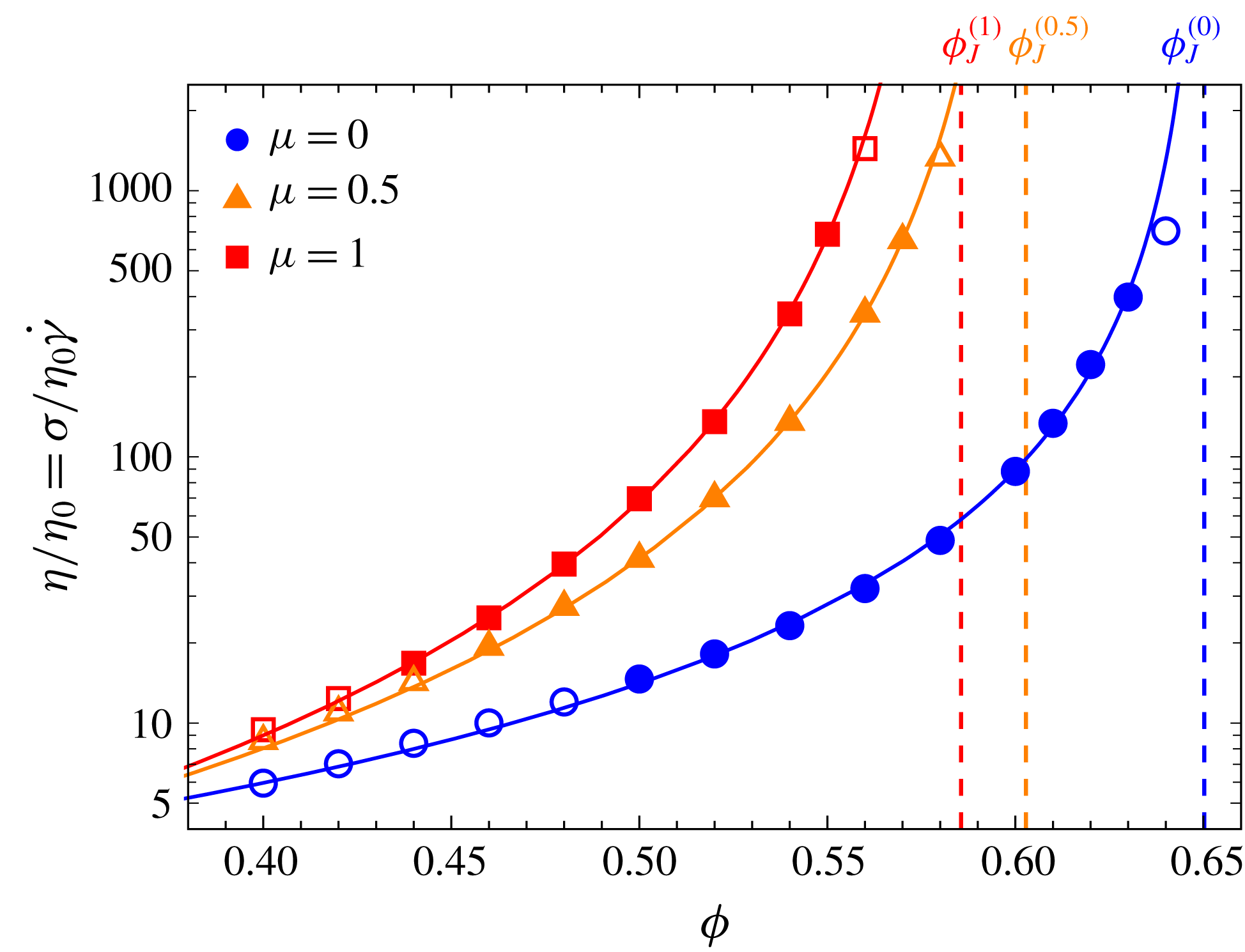
The relative viscosity
 $\unicode[STIX]{x1D702}/\unicode[STIX]{x1D702}_{0}$
diverges as the volume fraction
 $\unicode[STIX]{x1D719}$
approaches the jamming point
 $\unicode[STIX]{x1D719}_{J}^{(\unicode[STIX]{x1D707})}$
, a decreasing function of the friction coefficient
 $\unicode[STIX]{x1D707}$
. Solid lines are obtained by fitting
 $\unicode[STIX]{x1D702}/\unicode[STIX]{x1D702}_{0}=c(\unicode[STIX]{x1D719}_{J}-\unicode[STIX]{x1D719})^{-\unicode[STIX]{x1D706}}$
to the data with the filled symbols. Vertical dashed lines represent the values of
 $\unicode[STIX]{x1D719}_{J}^{(\unicode[STIX]{x1D707})}$
estimated from the fitting for each
 $\unicode[STIX]{x1D707}$
. The data corresponding to the open symbols near jamming are omitted in the fitting because of the potential inaccuracy due to the particle softness.
We work in the infinite-
 $Pe$
limit and we are interested in exploring the dependence of the rheology of dense suspensions on the volume fraction
 $\unicode[STIX]{x1D719}$
of solid particles dispersed in a Newtonian fluid with viscosity
 $\unicode[STIX]{x1D702}_{0}$
. The reported data are, unless specified otherwise, ensemble averages of time averages (taken in a statistically steady state) over 20 independent three-dimensional simulations of 1000 particles, with a bidisperse size distribution characterized by size ratio
 $1.4$
and volume ratio of approximately
 $1$
. The cutoff length employed to regularize the lubrication singularity is set to
 $\unicode[STIX]{x1D6FF}=10^{-3}a$
(Wilson & Davis Reference Wilson and Davis2002), with
 $a$
being the radius of the smaller particles. The parameter
 $k_{n}$
for the contact model is set to
 $10^{5}k_{0}$
, where the constant
 $k_{0}\equiv 6\unicode[STIX]{x03C0}\unicode[STIX]{x1D702}_{0}a\dot{\unicode[STIX]{x1D6FE}}$
is a reference value determined by the Stokes drag under a constant shear rate
 $\dot{\unicode[STIX]{x1D6FE}}$
. (Our simulation is analogous to rate-controlled rheological measurements, thus the shear rate
 $\dot{\unicode[STIX]{x1D6FE}}$
is constant over time.) The maximum particle displacement is set to
 $d_{max}=5\times 10^{-4}a$
and the time step adaptively computed as described above.
3.1 Geometric interpretation of
 $N_{1}$
and its presence in dense suspensions

As is well known, the relative viscosity
 $\unicode[STIX]{x1D702}/\unicode[STIX]{x1D702}_{0}$
is a monotonically increasing function of the volume fraction
 $\unicode[STIX]{x1D719}$
(figure 1). It follows the functional form
 $\unicode[STIX]{x1D702}(\unicode[STIX]{x1D719})/\unicode[STIX]{x1D702}_{0}=c(\unicode[STIX]{x1D719}_{J}-\unicode[STIX]{x1D719})^{-\unicode[STIX]{x1D706}}$
(solid lines in figure 1), featuring a power-law divergence at a jamming point
 $\unicode[STIX]{x1D719}_{J}$
that depends on the friction coefficient
 $\unicode[STIX]{x1D707}$
(vertical dashed lines in figure 1). As is expected in the presence of a similar divergence, we observe a growth of several orders of magnitude in the relative viscosity.
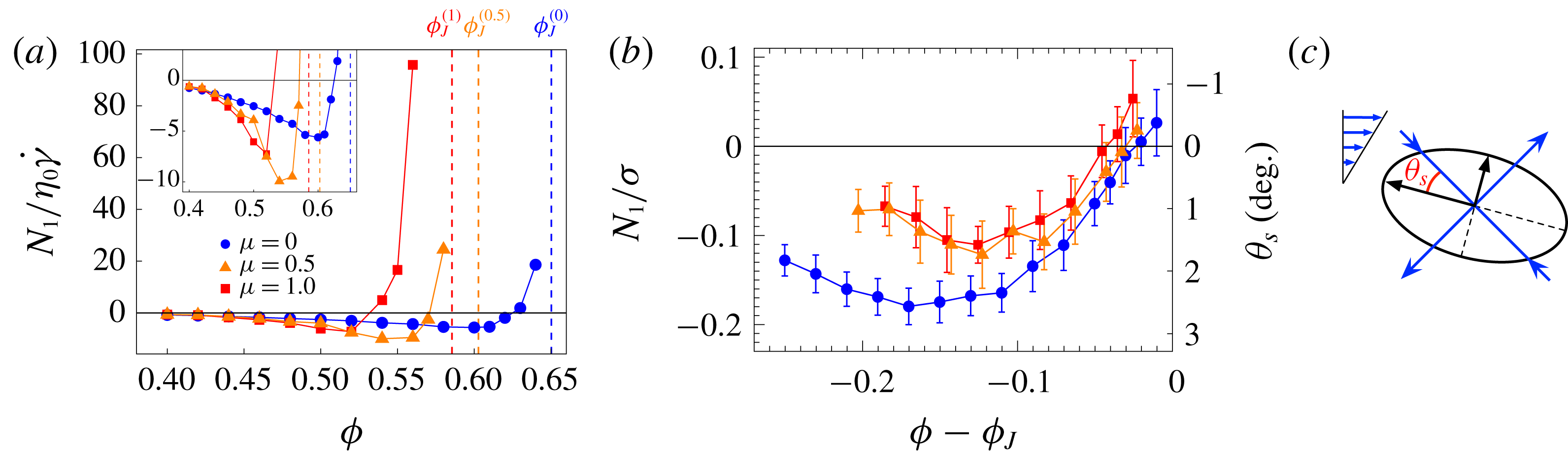
(a) The value of the normal stress difference
 $N_{1}$
divided by the solvent stress
 $\unicode[STIX]{x1D702}_{0}\dot{\unicode[STIX]{x1D6FE}}$
remains negative with an increasing intensity up to high volume fractions
 $\unicode[STIX]{x1D719}$
, where a sudden inversion towards large positive values is observed. The behaviour is similar for different values of the friction coefficient
 $\unicode[STIX]{x1D707}$
. Vertical dashed lines indicate the respective jamming points
 $\unicode[STIX]{x1D719}_{J}^{(\unicode[STIX]{x1D707})}$
. (b) The ratio between
 $N_{1}$
and the shear stress
 $\unicode[STIX]{x1D70E}$
or the corresponding reorientation angle
 $\unicode[STIX]{x1D703}_{s}$
give a better idea of the mildness of the effect measured by
 $N_{1}$
over the whole range of explored volume fractions. (c) The reorientation angle
 $\unicode[STIX]{x1D703}_{s}$
is defined as the angle, in the flow plane, between the eigenvectors of the stress tensor
 $\unicode[STIX]{x1D748}$
and the eigenvectors of
 $\unicode[STIX]{x1D63F}$
(oriented at
 $45^{\circ }$
from the flow direction).
By contrast, the
 $\unicode[STIX]{x1D719}$
-dependence of the first normal stress difference normalized by the solvent stress
 $\unicode[STIX]{x1D702}_{0}\dot{\unicode[STIX]{x1D6FE}}$
is non-monotonic: it is negative and slowly decreasing for moderate volume fractions, reaches a minimum and then rapidly increases to large positive values in the vicinity of the jamming point (figure 2
a). Nevertheless, a better appreciation of the role of
 $N_{1}$
and its rheological importance relative to that of the divergent viscosity comes from the analysis of the ratio
 $N_{1}/\unicode[STIX]{x1D70E}$
or the reorientation angle
 $\unicode[STIX]{x1D703}_{s}$
(figure 2
b). In fact, a non-vanishing
 $N_{1}$
indicates that the eigenvectors of the stress in the flow plane are rotated with respect those of
 $\unicode[STIX]{x1D63F}$
by an angle
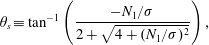 $$\begin{eqnarray}\unicode[STIX]{x1D703}_{s}\equiv \tan ^{-1}\left(\frac{-N_{1}/\unicode[STIX]{x1D70E}}{2+\sqrt{4+(N_{1}/\unicode[STIX]{x1D70E})^{2}}}\right),\end{eqnarray}$$
depicted in figure 2(c), which is determined only by the ratio
 $N_{1}/\unicode[STIX]{x1D70E}$
(Giusteri & Seto Reference Giusteri and Seto2018).
In terms of these quantities, the measured values of
 $N_{1}$
are seen to correspond to a minor rheological feature – at least an order of magnitude smaller than the shear stress – that varies smoothly with the volume fraction. Indeed,
 $N_{1}/\unicode[STIX]{x1D70E}$
is negative at lower volume fractions, decreases to a minimum and then gradually increases towards zero, turning to positive values only in close proximity to the jamming point (figure 2
b).
3.2 Synergy and competition between hydrodynamic and contact interactions
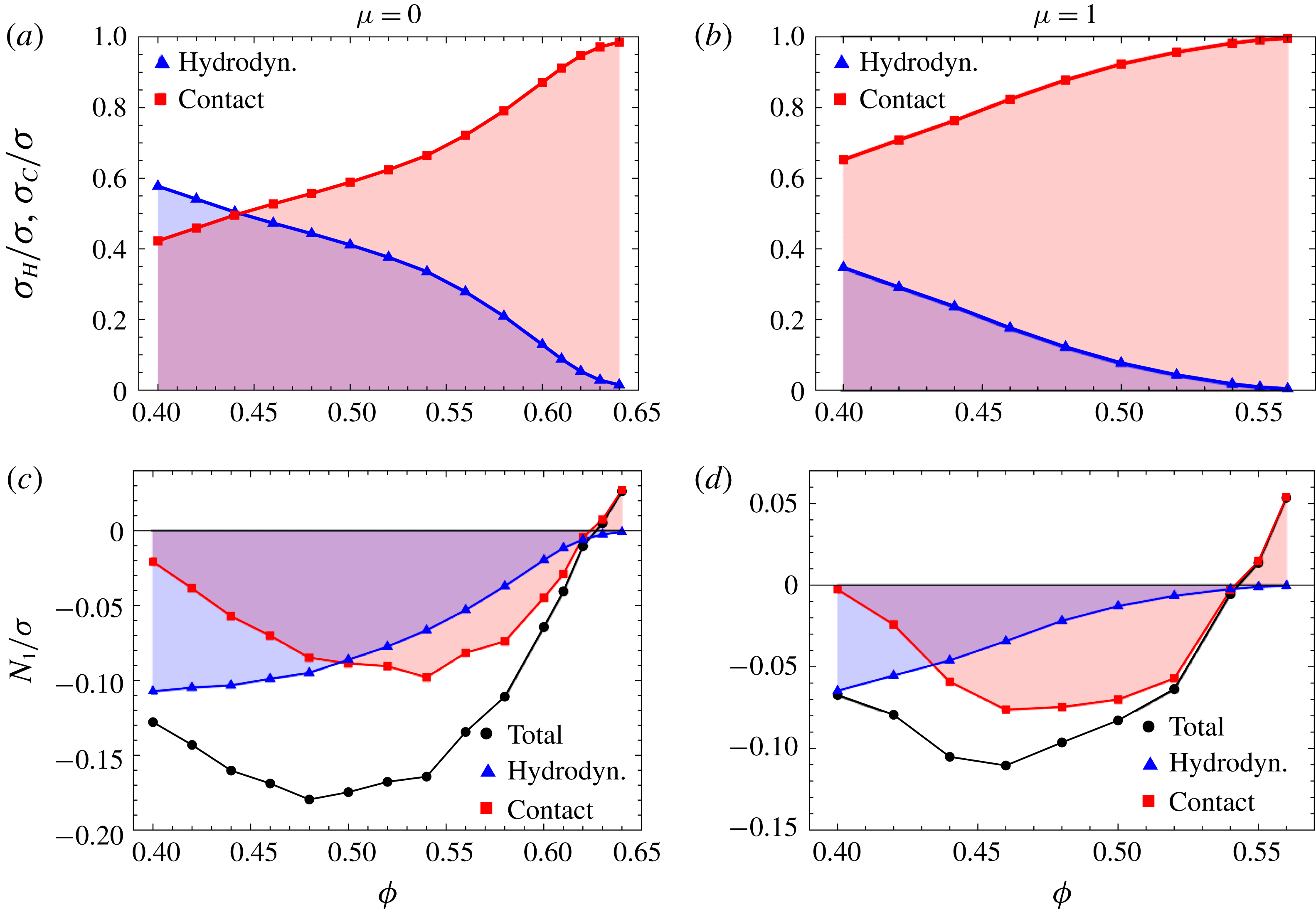
(a,b) The contact contribution
 $\unicode[STIX]{x1D70E}_{C}$
to the total shear stress
 $\unicode[STIX]{x1D70E}$
dominates the hydrodynamic one
 $\unicode[STIX]{x1D70E}_{H}$
over almost the whole range of explored volume fractions, both in the absence and presence of friction, even when hydrodynamic interactions determine a major fraction of
 $N_{1}$
. (c,d) Hydrodynamic and contact contributions to
 $N_{1}/\unicode[STIX]{x1D70E}$
for frictionless and frictional contacts are negative over a wide range of volume fractions
 $\unicode[STIX]{x1D719}$
. The hydrodynamic contribution decreases upon increasing
 $\unicode[STIX]{x1D719}$
. The negative contact contribution becomes dominant but then vanishes, before turning to positive values near the jamming point.
When discussing the
 $\unicode[STIX]{x1D719}$
-dependence of the viscosity and, through
 $N_{1}/\unicode[STIX]{x1D70E}$
, of the reorientation angle, it is instructive to break down the total values into hydrodynamic and contact contributions. This is possible by taking advantage of the ‘perfect knowledge’ offered by simulations, which is of course not available when treating experimental data. As for the viscosity, upon increasing the volume fraction contact interactions become more and more likely to occur and progressively hinder hydrodynamic interactions. We can pictorially say that the two effects ‘fight for space’ and the shear stress
 $\unicode[STIX]{x1D70E}$
is mostly determined by contact interactions. Moreover, as one would expect, the presence of friction enhances the preeminence of contacts (figure 3
a,b).
The situation for the ratio
 $N_{1}/\unicode[STIX]{x1D70E}$
is quite different (figure 3
c,d). At lower volume fractions the main contribution, with a negative sign, is given by hydrodynamic interactions, at intermediate volume fractions contacts begin to contribute, again with a negative sign, and the reorientation effect is strongest (
 $N_{1}/\unicode[STIX]{x1D70E}$
minimum) in a regime where the hydrodynamic contribution is still significant and the contact contribution is growing. After this synergic regime, both the hydrodynamic and contact contributions approach zero and, close to jamming, only the contact contribution survives and switches to a positive sign.
It is thus clear that the change in the sign of
 $N_{1}$
near the jamming point does not indicate the transition from a preeminence of contacts over hydrodynamic interactions, which mostly cooperate in building a microstructure that induces negative average contributions to
 $N_{1}$
.
3.3 From the microscopic force network to the macroscopic normal stress
We still need to understand what determines the sign of
 $N_{1}/\unicode[STIX]{x1D70E}$
. To this end, we introduce a simplified quantity that retains the basic features of
 $N_{1}$
. Any force between particles
 $i$
and
 $j$
can be decomposed into two parts, normal and tangential forces, by means of projections involving the normal vector
 $\boldsymbol{n}^{(ij)}\equiv (1/r_{ij})(\boldsymbol{r}^{(j)}-\boldsymbol{r}^{(i)})$
. Tangential contact forces play an essential role in the particle dynamics and rheology. Indeed, the friction coefficient
 $\unicode[STIX]{x1D707}$
shifts the jamming point and also determines the behaviour of
 $N_{1}$
as shown in § 3.1. However, we can verify that normal forces constitute the dominant part of the stress, and especially the contributions of the tangential forces to
 $N_{1}$
are very minor. Here, we introduce the reduced stress tensor including only normal forces,
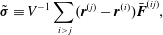 $$\begin{eqnarray}\tilde{\unicode[STIX]{x1D748}}\equiv V^{-1}\mathop{\sum }_{i>j}(\boldsymbol{r}^{(j)}-\boldsymbol{r}^{(i)})\bar{\boldsymbol{F}}^{(ij)},\end{eqnarray}$$
where
 $\bar{\boldsymbol{F}}^{(ij)}\equiv (\boldsymbol{F}^{(ij)}\boldsymbol{\cdot }\boldsymbol{n}^{(ji)})\boldsymbol{n}^{(ji)}=-\bar{F}_{ij}\boldsymbol{n}^{(ij)}$
is the normal force acting on particle
 $i$
from particle
 $j$
. Here, positive (respectively negative)
 $\bar{F}_{ij}$
gives a repulsive (respectively attractive) force. The reduced normal stress difference
 ${\tilde{N}}_{1}$
is defined as
 $$\begin{eqnarray}\displaystyle {\tilde{N}}_{1} & \equiv & \displaystyle \langle \tilde{\unicode[STIX]{x1D70E}}_{xx}-\tilde{\unicode[STIX]{x1D70E}}_{yy}\rangle \nonumber\\ \displaystyle & = & \displaystyle \langle V^{-1}\mathop{\sum }_{i>j}r_{ij}\bar{F}_{ij}[(n_{x}^{(ij)})^{2}-(n_{y}^{(ij)})^{2}]\rangle =\langle V^{-1}\mathop{\sum }_{i>j}(-r_{ij}^{\prime }\bar{F}_{ij}^{\prime }\sin 2\unicode[STIX]{x1D703}_{ij})\rangle =\langle \mathop{\sum }_{i>j}{\tilde{N}}_{1}^{ij}\rangle ,\nonumber\\ \displaystyle & & \displaystyle\end{eqnarray}$$
where the local angle
 $\unicode[STIX]{x1D703}_{ij}$
is the one formed between the projection of the normal vector
 $\boldsymbol{n}^{(ij)}$
in the flow plane and the compression axis. (Additionally,
 $r_{ij}^{\prime }$
and
 $F_{ij}^{\prime }$
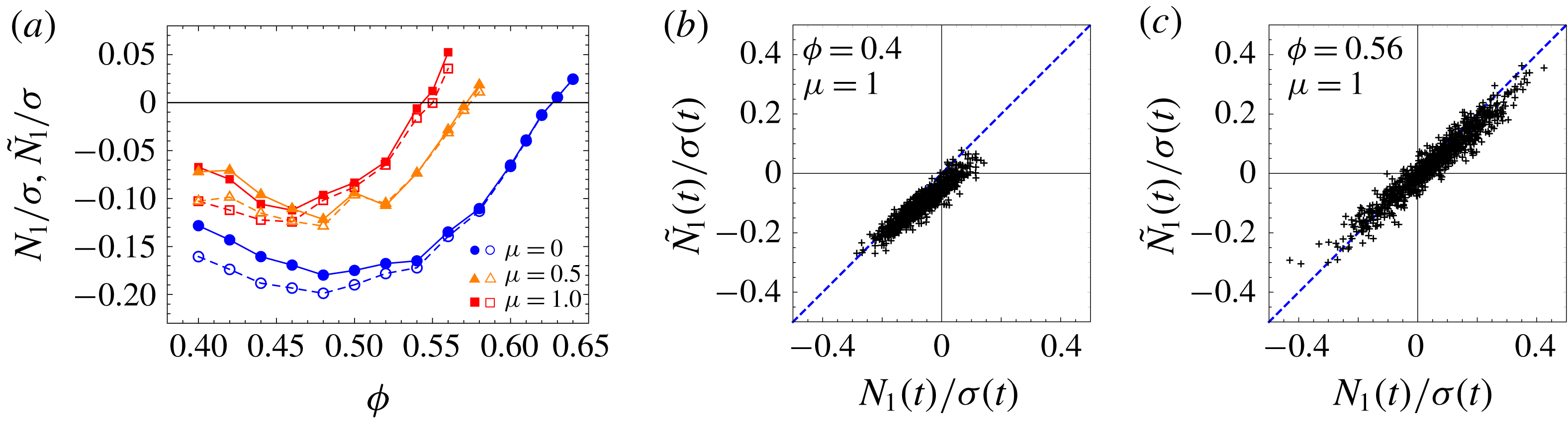
are norms of the projected vectors on the plane.) By analysing the data from our simulations, we can confirm that not only is
 ${\tilde{N}}_{1}$
a good approximation of
 $N_{1}$
(figure 4
a), but even the instantaneous value
 $N_{1}(t)$
can be reasonably reproduced by the reduced
 ${\tilde{N}}_{1}(t)$
, especially at higher volume fractions where the contact forces are predominant, as seen in figure 4(b).
(a) The reduced normal stress difference
 ${\tilde{N}}_{1}$
(open symbols) constructed by omitting tangential lubrication and contact forces can reproduce
 $N_{1}$
(solid symbols), especially at higher volume fractions. (b) Even the instantaneous value
 ${\tilde{N}}_{1}(t)$
linearly correlates with
 $N_{1}(t)$
.
To illustrate how the local contributors
 ${\tilde{N}}_{1}^{ij}$
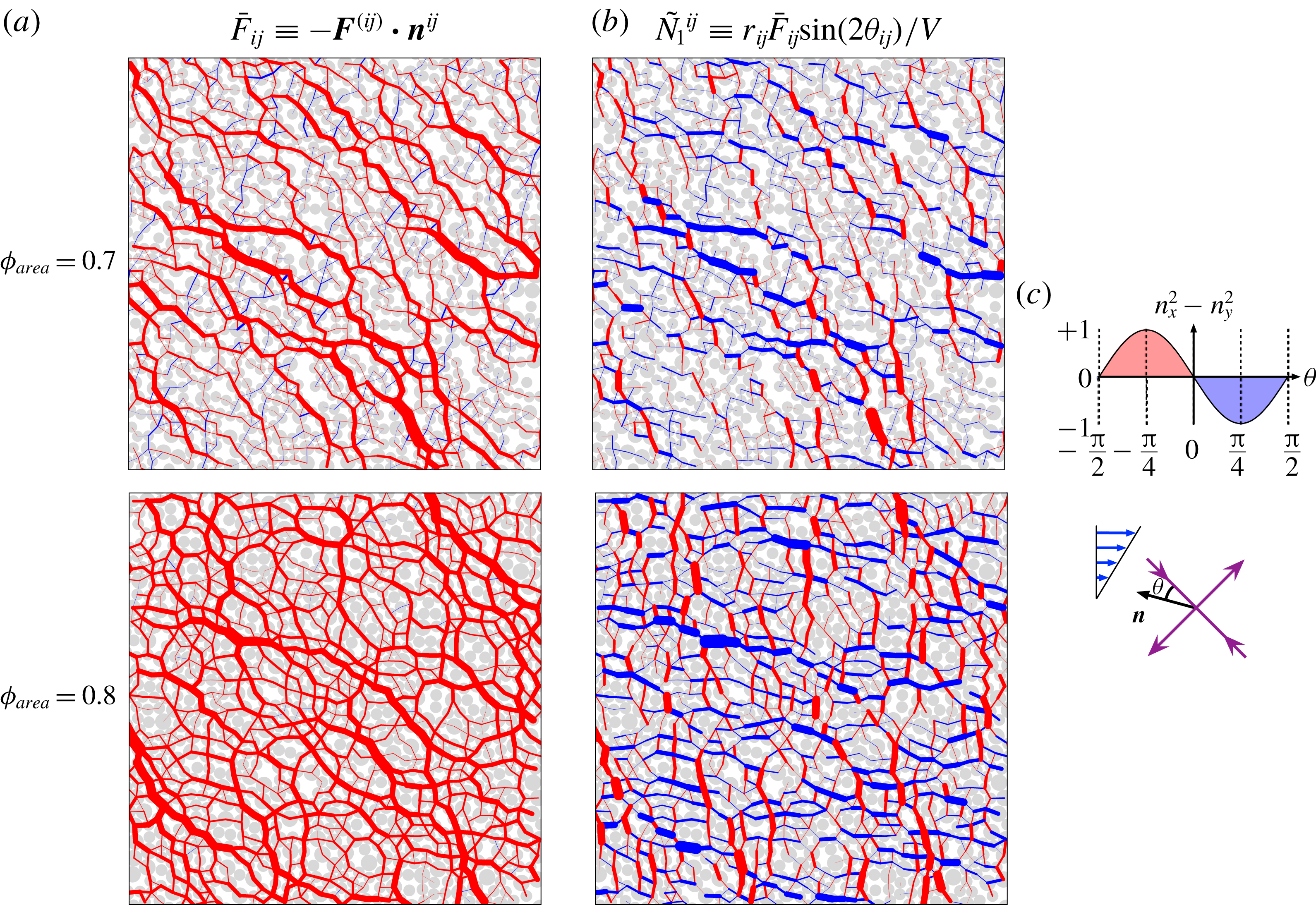
relates to the force network, we perform some two-dimensional (2-D) monolayer simulations, which retain the qualitative features of the 3-D simulations while allowing for an easier visual perception, that can guide our understanding of the microscopic interactions. Figure 5(a) presents typical snapshots of the force network for a frictional system (
 $\unicode[STIX]{x1D707}=0.5$
) at area fraction
 $\unicode[STIX]{x1D719}_{area}=0.7$
(upper panel) and
 $\unicode[STIX]{x1D719}_{area}=0.8$
(lower panel). Normal forces
 $\bar{\boldsymbol{F}}^{(ij)}$
between interacting pairs are drawn as segments. The red and blue colours indicate repulsive and attractive forces. The strength of the normal forces is visualized by varying the thickness of the segments. We see that the most significant normal forces in these snapshots are repulsive (red).
(a) Snapshots of 2-D monolayer simulations to show the force network of the pairwise normal force
 $\bar{\boldsymbol{F}}^{(ij)}$
. The thickness of the segments indicates the intensity of the force. Repulsive forces (
 $\bar{F}_{ij}>0$
) are in red and attractive forces (
 $\bar{F}_{ij}<0$
) in blue. (b) The pairwise local contributions
 ${\tilde{N}}_{1}^{ij}$
to the first normal stress difference. The vertical repulsive forces contribute positively (red), and the horizontal ones negatively (blue). (c) Illustration of the factor
 $n_{x}^{2}-n_{y}^{2}$
, that determines the sign of
 ${\tilde{N}}_{1}^{ij}$
, in terms of the local orientation angle
 $\unicode[STIX]{x1D703}$
formed by the normal force and the compression axis.
The local contributors
 ${\tilde{N}}_{1}^{ij}$
to the reduced normal stress difference
 ${\tilde{N}}_{1}(t)$
are represented in a similar manner in figure 5(b). They contain the normal force
 $\bar{F}_{ij}$
as a factor (see (3.3)), but it is the factor
 $n_{x}^{2}-n_{y}^{2}$
(a function of the local angle
 $\unicode[STIX]{x1D703}_{ij}$
) that decides the sign of the contribution to
 ${\tilde{N}}_{1}(t)$
, as shown in figure 5(c). (We observe that
 ${\tilde{N}}_{1}(t)$
is negative at
 $\unicode[STIX]{x1D719}_{area}=0.7$
and positive at
 $\unicode[STIX]{x1D719}_{area}=0.8$
.) When two particles align along the compression axis (
 $\unicode[STIX]{x1D703}_{ij}=0$
), the normal force does not contribute to
 ${\tilde{N}}_{1}$
at all. The instantaneous value of
 ${\tilde{N}}_{1}$
is given by the sum of many contributions, from all the particle pairs, with opposite sign. Indeed, in a typical snapshot, we can find strong local contributions of both positive (red) and negative (blue) sign.
A more quantitative understanding of this observation can be reached by evaluating the time-averaged distribution of the normal forces and the normal stress components,
 $\bar{F}_{ij}$
and
 ${\tilde{N}}_{1}^{ij}$
, in terms of the local angle
 $\unicode[STIX]{x1D703}$
for 3-D simulations. Figure 6(a) shows the distribution
 $\langle \bar{F}(\unicode[STIX]{x1D703})\rangle$
of the normal forces divided by the maximum value
 $\bar{F}_{max}$
. The peaks of the force distributions are found around the compression axis (
 $\unicode[STIX]{x1D703}=0$
). This confirms that, although we can find some attractive forces (negative values) along the extension axis at lower values of
 $\unicode[STIX]{x1D719}$
, the significant normal forces are mostly repulsive.
The significant normal forces are mostly repulsive and the time-averaged values of
 $N_{1}/\unicode[STIX]{x1D70E}$
are the result of cancellations among local contributions of opposite sign. This can be seen from the angular distributions of (a) the projected normal force
 $\langle \bar{F}(\unicode[STIX]{x1D703})\rangle$
on the flow plane and (b) the ratio
 ${\tilde{N}}_{1}(\unicode[STIX]{x1D703})/\unicode[STIX]{x1D70E}$
, obtained from 3-D simulations with friction coefficient
 $\unicode[STIX]{x1D707}=1$
.
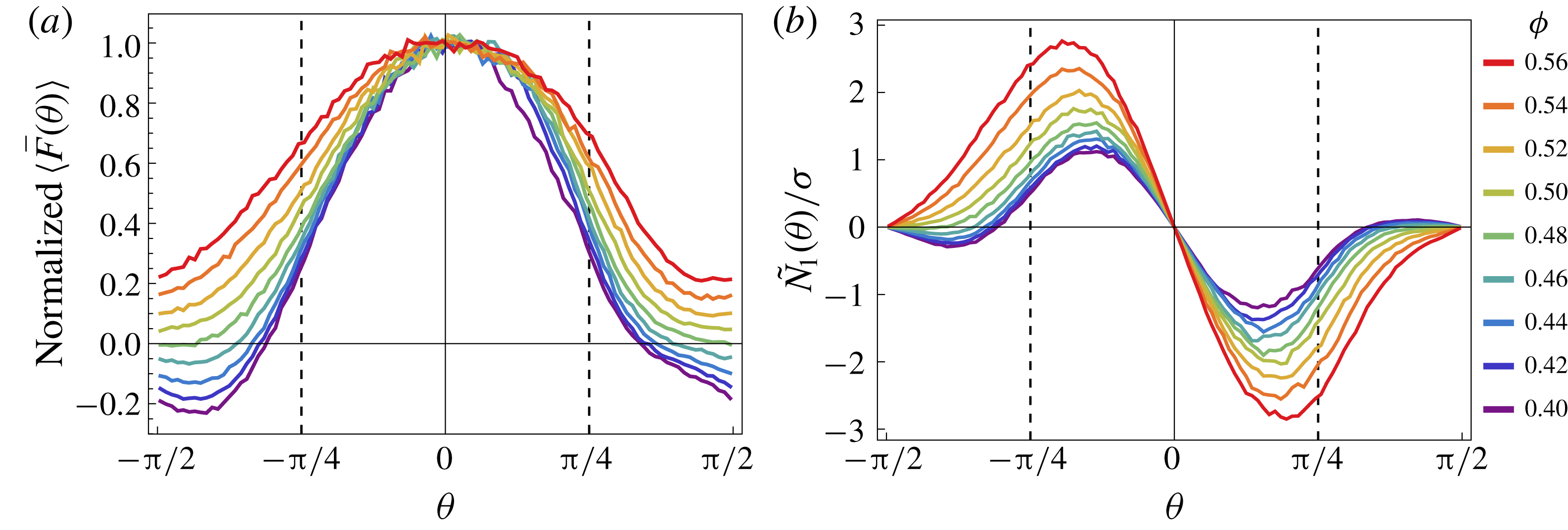
The angular distributions
 ${\tilde{N}}_{1}(\unicode[STIX]{x1D703})/\unicode[STIX]{x1D70E}$
in figure 6(b) show very prominent positive and negative peaks. Nevertheless, the global value of
 ${\tilde{N}}_{1}/\unicode[STIX]{x1D70E}$
, obtained by integrating
 ${\tilde{N}}_{1}(\unicode[STIX]{x1D703})/\unicode[STIX]{x1D70E}$
over the entire range of directions, is somehow small with large fluctuations over time. The fact that the global values are the result of a cancellation between large contributions of opposite signs makes the sign of its fluctuating instantaneous values uncertain.
We can conclude that a global non-vanishing value of
 $N_{1}$
is generated by a small imbalance of positive and negative contributions in the angular distributions presented above. This is associated with a mild preference of the dominant branches of the force network to be aligned along a direction different from the compression axis defined by the shear flow.
3.4 Anisotropy due to the planarity of the flow
As mentioned in the introductory section, the stress tensor in steady simple shear is characterized by three degrees of freedom. So far, we have discussed the
 $\unicode[STIX]{x1D719}$
-dependence of the viscosity
 $\unicode[STIX]{x1D702}=\unicode[STIX]{x1D70E}/\dot{\unicode[STIX]{x1D6FE}}$
and the first normal stress difference
 $N_{1}$
. The third degree of freedom is normally associated with the second normal stress difference
 $N_{2}$
but, as shown by Giusteri & Seto (Reference Giusteri and Seto2018), this quantity is not fully independent of
 $N_{1}$
, since it is a combined measure of the misalignment between
 $\unicode[STIX]{x1D748}$
and
 $\unicode[STIX]{x1D63F}$
(already captured by
 $N_{1}$
) and of a second effect. The latter corresponds to a stress contribution which is isotropic in the flow plane (i.e. the
 $x$
–
 $y$
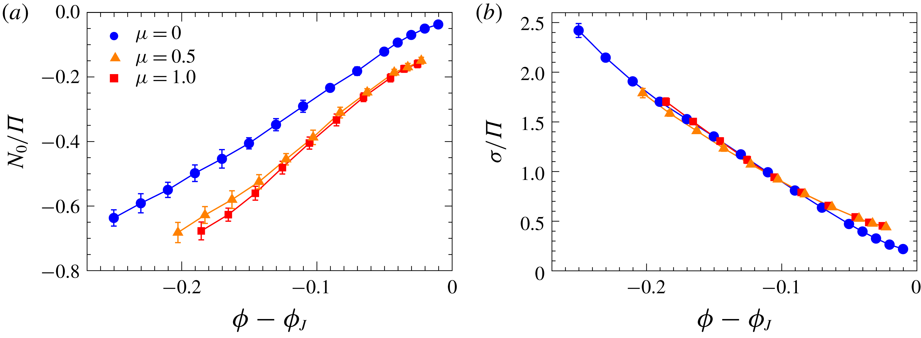
plane) but globally anisotropic, when the vorticity direction is taken into account. In a simple shear flow, the non-vanishing vorticity is everywhere orthogonal to the flow plane and the invariance under any translation along this direction characterizes the planarity of such flows. A good measure of the third independent degree of freedom is given by
 $$\begin{eqnarray}N_{0}\equiv \left\langle \frac{\unicode[STIX]{x1D70E}_{xx}+\unicode[STIX]{x1D70E}_{yy}}{2}-\unicode[STIX]{x1D70E}_{zz}\right\rangle =N_{2}+\frac{N_{1}}{2}.\end{eqnarray}$$
 $N_{0}$
is normalized by the isotropic pressure
 $\unicode[STIX]{x1D6F1}\equiv -(1/3)\langle \text{Tr}\unicode[STIX]{x1D748}\rangle$
, so that
 $N_{0}/\unicode[STIX]{x1D6F1}$
can be understood by considering that it reflects an anisotropy of the normal stress (or ‘pressure’) originating from the planarity of the flow. The negative values of
 $N_{0}/\unicode[STIX]{x1D6F1}$
in figure 7(a) indicate that the flow generates more ‘pressure’ in the flow plane than in the vorticity direction. This anisotropy monotonically decreases as the system becomes denser and denser, and the viscosity higher and higher (see figure 1). In the limit where the viscosity of frictionless systems (
 $\unicode[STIX]{x1D707}=0$
) diverges, the anisotropy looks to vanish. This is consistent with the idea that flow-induced microstructures are not relevant to frictionless jamming, this being dominated by geometric effects. On the other hand, a residual stress anisotropy survives in the limit of jamming with friction
 $\unicode[STIX]{x1D707}>0$
. Indeed, it has been suggested that flow-induced microstructures may contribute to the jamming of frictional systems (Cates et al.
Reference Cates, Wittmer, Bouchaud and Claudin1998; Bi et al.
Reference Bi, Zhang, Chakraborty and Behringer2011). A similar observation was also reported as ‘absence of dilatancy’ in the quasi-static limit of frictionless granular flows (Peyneau & Roux Reference Peyneau and Roux2008).
To complete our discussion of the stress anisotropy, we now consider the anisotropy generated in the flow plane by the shear flow itself. This is of course a dominant effect in shear rheology and it can be measured by the ratio of the shear stress
 $\unicode[STIX]{x1D70E}=\unicode[STIX]{x1D702}\dot{\unicode[STIX]{x1D6FE}}$
to
 $\unicode[STIX]{x1D6F1}$
, a quantity that defines the macroscopic friction coefficient in the context of granular flows (Boyer, Guazzelli & Pouliquen Reference Boyer, Guazzelli and Pouliquen2011a
). The ratio
 $\unicode[STIX]{x1D70E}/\unicode[STIX]{x1D6F1}$
displays a decreasing trend upon increasing the volume fraction, but a finite anisotropy seems to survive even in the proximity of jamming (figure 7
b). Notably, for a range of volume fractions that are not too close to the jamming point, the data for different friction coefficients collapse on the same curve. This points to a geometric origin of this anisotropy in dense suspensions, that makes it insensitive to friction, which is in turn essential in determining dynamical properties of the system such as the intensity of the stress response. Nevertheless, close to jamming we observe a measurable difference in the residual anisotropy for frictional and frictionless systems. Such difference seems equivalent to what is observed in the quasi-static limit of granular dynamics, that is
 $\unicode[STIX]{x1D70E}/\unicode[STIX]{x1D6F1}\sim 0.1$
for
 $\unicode[STIX]{x1D707}=0$
(Peyneau & Roux Reference Peyneau and Roux2008) and
 $\unicode[STIX]{x1D70E}/\unicode[STIX]{x1D6F1}\sim 0.35$
for
 $\unicode[STIX]{x1D707}>0.4$
(Singh, Magnanimo & Luding Reference Singh, Magnanimo and Luding2013; Azéma & Radjaï Reference Azéma and Radjaï2014).
(a) The absolute value of the ratio
 $N_{0}/\unicode[STIX]{x1D6F1}$
, a measure of the anisotropy of the stress in the vorticity direction, decreases upon increasing the volume fraction
 $\unicode[STIX]{x1D719}$
since the force network becomes more and more isotropic as the jamming point is approached. For frictional systems, a residual anisotropy is observed. (b) The ratio of
 $\unicode[STIX]{x1D70E}$
to
 $\unicode[STIX]{x1D6F1}$
, a measure of the anisotropy in the flow plane, also decreases with
 $\unicode[STIX]{x1D719}$
. The data for different values of the friction coefficient
 $\unicode[STIX]{x1D707}$
display a nice collapse as a function of
 $\unicode[STIX]{x1D719}-\unicode[STIX]{x1D719}_{J}$
, except for the points close to the jamming condition.
3.5 The role of elastic effects near jamming
In view of the link we established between the microscopic properties of the force network and the macroscopic value of
 $N_{1}$
, the presence of a non-vanishing
 $N_{1}$
near jamming appears to be puzzling, irrespective of its sign. In the limit of jamming with hard spheres, we expect that effects of the rotational component of the flow are negligible compared to those of the extensional component (Seto et al.
Reference Seto, Giusteri and Martiniello2017). If so, the force network would become statistically symmetric across the compression axis in the flow plane, entailing a vanishing
 $N_{1}$
. Nevertheless, our data indicate the presence of a symmetry breaking measured by non-zero values of
 $N_{1}$
. We thus need to identify some factor that has been ignored in our previous arguments.
In analogy with what happens in viscoelastic fluids, the symmetry could be broken by the vorticity if some elastic links were actually convected by the flow. While there is no such link in a hard-sphere suspension, the contact model employed in our simulation effectively approximates hard spheres with high-stiffness elastic ones. We then argue that the observed positive values of
 $N_{1}$
are due to a failure of the simulation strategy in resolving contacts in a sufficiently rapid way. Particles that overlap significantly for some time produce normal forces with directions that are rotated towards the gradient direction, inducing an average reorientation of the stress eigenvectors.
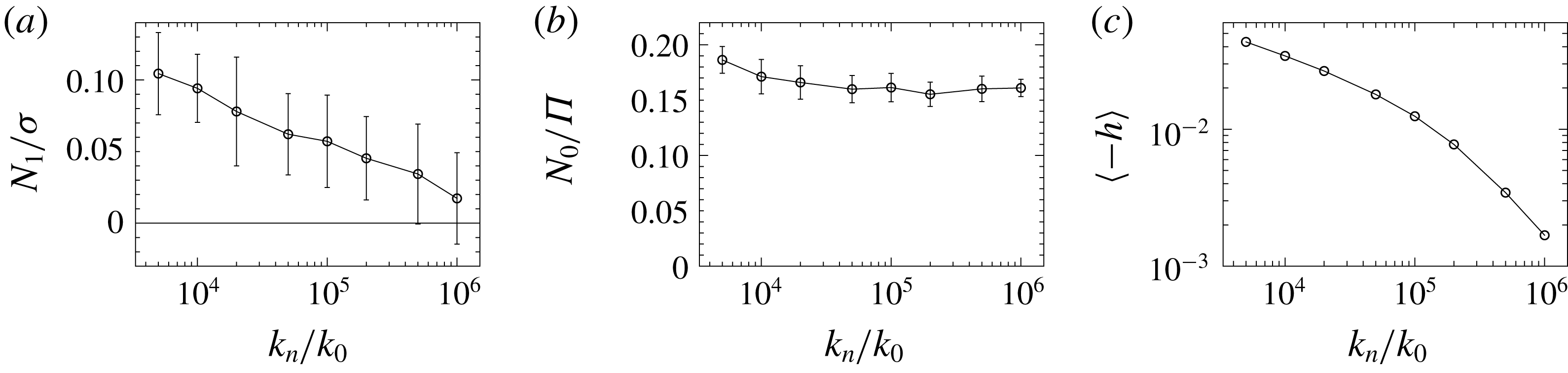
To confirm this interpretation, we analysed the dependence of
 $N_{1}/\unicode[STIX]{x1D70E}$
on the effective normal stiffness
 $k_{n}$
of the frictional contact model (
 $\unicode[STIX]{x1D707}=1$
) by running 20 independent 3-D simulations for each value of
 $k_{n}$
at the volume fraction
 $\unicode[STIX]{x1D719}=0.56$
, which is close to jamming and gave a positive value of
 $N_{1}$
in the data reported above. (The maximum displacement is set to a common constant value
 $d_{max}=5\times 10^{-4}a$
for
 $k_{n}\leqslant 10^{5}k_{0}$
and, to ensure the reliability of the simulations, reduced in inverse proportion to
 $k_{n}$
for stiffer particles with
 $k_{n}>10^{5}k_{0}$
.) Even though we cannot test extremely large values of
 $k_{n}$
(the time steps would get extremely short and the simulation time diverge) we found a clear trend of
 $N_{1}/\unicode[STIX]{x1D70E}$
decreasing as
 $k_{n}$
increases (figure 8
a). We may infer that, in the hard-sphere limit,
 $N_{1}/\unicode[STIX]{x1D70E}$
is negative below jamming and asymptotically approaches zero at the jamming point. In the same conditions, the value of
 $N_{0}/\unicode[STIX]{x1D6F1}$
is not affected by the tested increase in
 $k_{n}$
(figure 8
b). This means that the finite stress anisotropy observed near the frictional jamming and due to the planarity of shear flows is not an artefact of the simulation but a genuine phenomenon.
(a) The positive value of
 $N_{1}/\unicode[STIX]{x1D70E}$
, observed at the volume fraction
 $\unicode[STIX]{x1D719}=0.56$
with friction coefficient
 $\unicode[STIX]{x1D707}=1$
, decreases if we increase the elastic constant
 $k_{n}$
employed in the contact model to approximate the hard-sphere interaction. This indicates such elastic interactions as the origin of the positive
 $N_{1}$
near jamming. (b) The observed value of
 $N_{0}/\unicode[STIX]{x1D6F1}$
is not significantly affected by changes in
 $k_{n}$
over the explored range. (c) The dependence of the average maximum overlap
 $\langle -h\rangle$
on
 $k_{n}$
indicates that our simulation is gradually approaching the hard-sphere limit as the elastic constant
 $k_{n}$
increases.
Based on the awareness we gained from the computational results for stiffer particles, we can make an instructive comparison with experimental studies. We take the work by Royer et al. (Reference Royer, Blair and Hudson2016) as an example. In these experiments, a suspension of silica particles with
 $2a=1.54~\unicode[STIX]{x03BC}\text{m}$
is fully thickened under a shear stress of 6000 Pa and exhibits a positive
 $N_{1}$
for volume fractions above
 $\unicode[STIX]{x1D719}=0.54$
. The typical contact deformation in such situation can be estimated as
 $10^{-4}a$
, by using the Hertzian contact model
 $F=(4/3)E^{\ast }a^{1/2}h^{3/2}$
with an effective elastic modulus
 $E^{\ast }=E/2(1-\unicode[STIX]{x1D708}^{2})$
given by assuming Young’s modulus
 $E=70~\text{GPa}$
and Poisson ratio
 $\unicode[STIX]{x1D708}=0.17$
of silica particles. Such average overlaps can be realized with
 $k_{n}/k_{0}\approx 10^{7}$
in our simulation, if the results of figure 8(c) are simply extrapolated. For such stiff particles, the computational value of
 $N_{1}/\unicode[STIX]{x1D70E}$
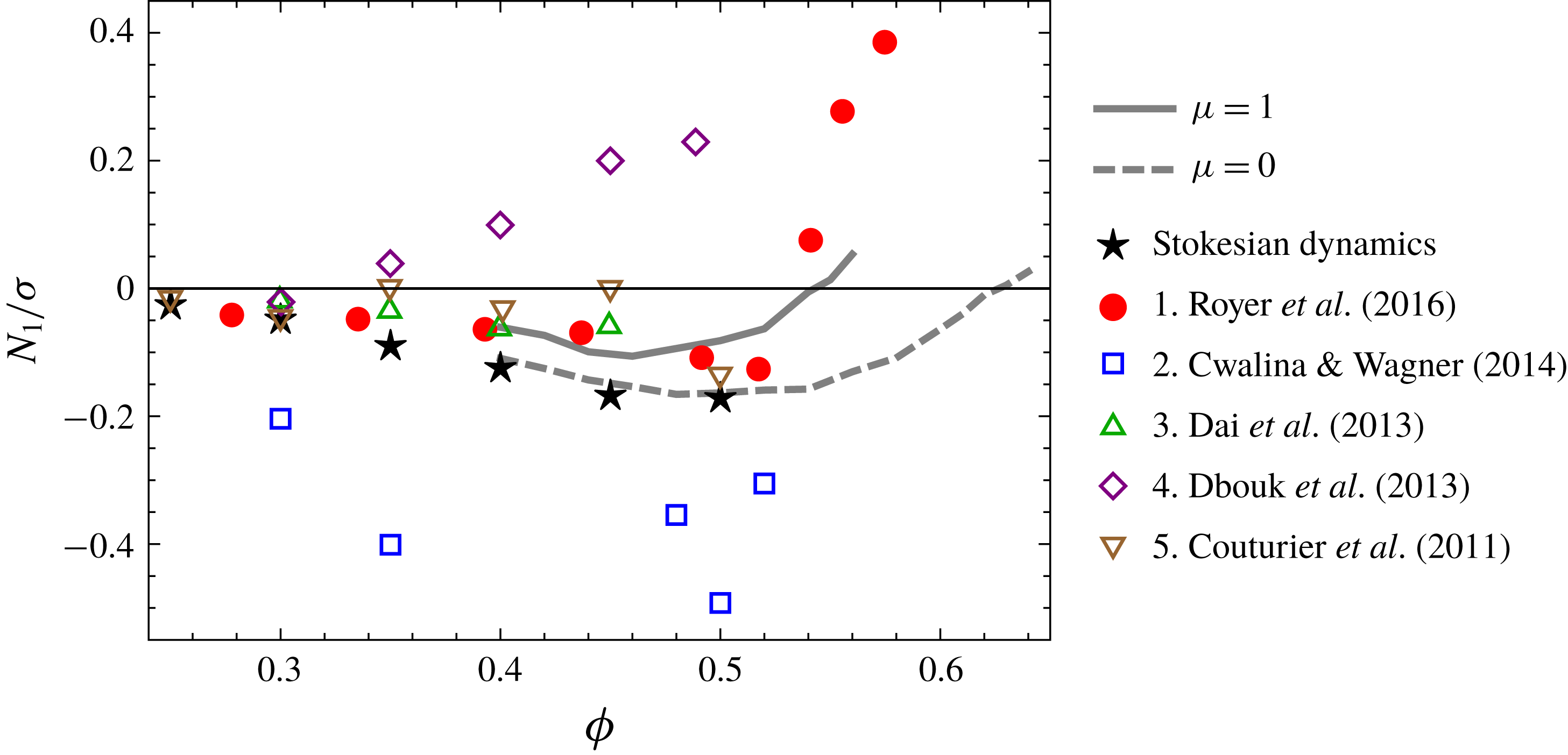
is expected to be vanishing or slightly negative from extrapolating the data presented in figure 8(a). Nevertheless, the data from Royer et al. (Reference Royer, Blair and Hudson2016), red circles in figure 9, show definitely positive values of
 $N_{1}/\unicode[STIX]{x1D70E}$
. The discrepancy between simulations and experiments can be explained either with the presence of interactions absent from our model, if it concerns bulk rheology, or as a signature of boundary effects due to the presence of walls in standard rheometers. Indeed, Gallier et al. (Reference Gallier, Lemaire, Lobry and Peters2016) numerically investigated wall effects on
 $N_{1}$
and found that
 $N_{1}/\unicode[STIX]{x1D70E}$
can be largely positive due to wall-induced ordering.
4 Conclusions
We investigated, by means of particle dynamics simulations, the presence and the microscopic origin of normal stress differences in dense suspensions under simple shear flows in the high-Péclet-number limit. By interpreting the first normal stress difference
 $N_{1}$
as a measure of the misalignment between the stress
 $\unicode[STIX]{x1D748}$
and the symmetric part of the velocity gradient
 $\unicode[STIX]{x1D63F}$
, we have shown that it represents a minor effect in comparison to the increment in the viscous response due to the interactions among the dispersed particles. Importantly, we provided evidence that the sign of
 $N_{1}$
cannot be used to discriminate whether hydrodynamic or contact interactions are dominant. In fact, in the dense regime, hydrodynamic and contact interactions always cooperate to give negative contributions to
 $N_{1}$
. From our analysis, it appears how the properties of the force network generated under shear are key to understanding the rheology of the system. Indeed, the observed misalignment is so mild because it originates from a small imbalance of intense but competing local contributions, that cancel each other in the macroscopic average.
Moreover, microscopic arguments allow us to understand the meaning of positive values of
 $N_{1}$
. For hard-sphere suspensions close to the jamming condition the force network becomes symmetric across the compression axis in the flow plane, implying a vanishing
 $N_{1}$
. This is a clear discrepancy with the positive values of
 $N_{1}$
found in some experiments. We argue that those values ought to be traced back to effects that cannot be accounted for with simple hard-sphere models. In fact, we show that the positive values obtained in our simulations are due to the presence of elastic interactions employed to regularize the (numerically stiff) hard-sphere constraint. A possible explanation of the experimental results could be sought in the presence of persistent elastic interactions between particle pairs that are advected by the flow. However, as shown in figure 9, definitely positive values of
 $N_{1}/\unicode[STIX]{x1D70E}$
near jamming are found in experiments with particles that are much stiffer than in our simulation, such as those by Royer et al. (Reference Royer, Blair and Hudson2016). This may suggest boundary effects due to the presence of walls in experiments, rather than bulk rheological properties, as an alternative explanation for the observed positive values of
 $N_{1}/\unicode[STIX]{x1D70E}$
.
Comparison of our simulation results for the cases
 $\unicode[STIX]{x1D707}=1$
(solid grey line) and
 $\unicode[STIX]{x1D707}=0$
(dashed grey line) with some reported experiments from the literature. Our frictionless simulation agrees with the Stokesian dynamics by Sierou & Brady (Reference Sierou and Brady2002), indicating that the lubrication approximation is justified at such high volume fractions. The frictional simulation near jamming shows a value of
 $N_{1}/\unicode[STIX]{x1D70E}$
much closer to zero than the reported experimental data, suggesting that some effects are being neglected in the computational model. The material and diameter of the particles used in the experiments are: 1. silica,
 $1.54~\unicode[STIX]{x03BC}\text{m}$
; 2. silica,
 $0.52~\unicode[STIX]{x03BC}\text{m}$
; 3. polystyrene,
 $40~\unicode[STIX]{x03BC}\text{m}$
; 4. polystyrene,
 $40~\unicode[STIX]{x03BC}\text{m}$
; 5. polystyrene,
 $140~\unicode[STIX]{x03BC}\text{m}$
.
In place of the second normal stress difference
 $N_{2}$
, we studied the quantity
 $N_{0}\equiv N_{2}+N_{1}/2$
. This measures an effect genuinely independent of the misalignment measured by
 $N_{1}$
, namely a stress contribution isotropic in the flow plane but globally anisotropic. It reflects an anisotropy in the force network originating from the planarity of the flow. The force network tends to be isotropic near jamming for frictionless contacts, and
 $N_{0}$
vanishes accordingly, but some residual anisotropy is observed near jamming for the case of frictional contacts.
In this work, we restricted our attention to the high-Péclet-number limit, where only hydrodynamic and contact forces determine the particle dynamics. Under lower stresses, some other force, such as Brownian forces or short-range repulsive forces, tends to prevent contact and to maintain a lubrication layer between particles. Such lubricated contacts are more similar to those obtained in the frictionless system. Under higher stresses, the effect of the additional force declines and frictional contacts appear. As a consequence of this mechanism, the shear thickening of dense suspensions, a rate-dependent feature, can be reproduced by interpolating between two points on the rate-independent frictionless and frictional rheology curves in figure 1 with a function of a state parameter that controls the effective jamming point (Wyart & Cates Reference Wyart and Cates2014; Singh et al.
Reference Singh, Mari, Denn and Morris2018). Analogously, a possible way to predict the rate dependence of
 $N_{1}/\unicode[STIX]{x1D70E}$
would involve interpolating the reported results for frictionless and frictional systems. Nevertheless, the non-monotonic behaviour of
 $N_{1}$
makes it harder to find a suitable interpolating function.
Acknowledgements
This study was supported by Japan Society for the Promotion of Science (JSPS) KAKENHI grants no. JP17K05618 and New Energy and Industrial Technology Development Organization of Japan (NEDO) grant no. P16010. The research of R.S. was also supported in part by the National Science Foundation under grant no. NSF PHY17-48958. The authors would like to thank the participants of the KITP program ‘Physics of Dense Suspensions’ for the many fruitful discussions and A. Singh, L. Hsiao, M. Denn and J. Morris for providing useful comments on the manuscript.


 Open access

