DATA AND METHODOLOGY

The main data source for this project is the Course of the Exchange, which from the beginning of the nineteenth century was regarded as the official price list for the London Stock Exchange.Footnote ⁷ Up until 1843 it was published in London twice weekly, and from then on it was published daily. We obtained a duplicate of the British Library's microfilm copy of this publication, which covers the period from March 1825 onwards. The Course of the Exchange reports the following for each stock: the number of issued shares, the nominal and paid-up (or par) value of shares, the dividend paid by the stock, and a share price if trade had taken place in the company's stock.

Our sample period begins in 1825 because this marks the beginning of the liberalization of incorporation law in Britain. Furthermore, prior to this period the performance of joint-stock companies was closely tied to that of the government, because such companies were often part of the government's politico-economic apparatus, e.g., Bank of England and East India Company.Footnote ⁸ For this reason, these two companies are excluded from our sample.Footnote ⁹

We manually collected the last share price of the month for all common equity stocks reported in the Course of the Exchange, working our way methodically through each month.Footnote ¹⁰ The small number of colonial and foreign railways listed in the Course of the Exchange is excluded because it is difficult to tell whether securities are debt, common equity, or preference shares. Thankfully, The Railway Times enabled us to verify the nature of British railway securities. In our sample period, there were 1,119 different companies and 1,657 different common equity securities listed in the Course of the Exchange.

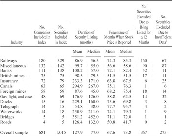
Unlike previous indices, ours includes all stocks reported in the Course of the Exchange with several exceptions. First, stocks which were listed for less than 12 months were excluded since it is doubtful whether these companies really got off the ground. As can be observed from Table 1, nearly half of those companies excluded on this criterion were railways. Second, 100 companies were excluded because no capitalization data (i.e., number of issued shares, nominal or paid-up value) was reported for the stock in the Course of the Exchange.Footnote ¹¹

Table 1

AN ANALYSIS OF THE COMPANIES AND SECURITIES INCLUDED IN AND EXCLUDED FROM OUR INDICES

¹ If less than 10 percent of months had prices reported, the security was excluded. Companies with no capitalization data were also excluded.

Source:

See the text.

Third, stocks were excluded if prices were reported for less than 10 percent of their listing duration. This condition excludes infrequently traded stocks, which were typically issued by very small companies. Using this criterion, we excluded 175 stocks.Footnote ¹² As can be seen from Table 1, after applying all the above criteria, we had data on 1,015 securities for 681 companies.

The relative illiquidity of the nineteenth-century stock market meant that in some months no trades took place, and hence no stock prices were reported in the Course of the Exchange. As can be seen from Table 1, on average, stock prices were reported for 67.6 percent of the months for which a stock was listed. If there was no stock price reported in a particular month or for several months and the stock was still listed, we assumed that the last reported price was the current stock price for the month, and if no stock price was reported for 48 consecutive months or more, we assumed that the company didn't exist for this period. In order to check for the robustness of this methodology, we also calculated returns whenever having no share price reported meant that that particular stock was omitted from our calculations. This approach has virtually no effect on our average return estimates, although, unsurprisingly, the standard deviation is slightly higher.

The Course of the Exchange reported annual or semiannual dividends in each issue as a percentage of paid-up capital or as dividend per share.Footnote ¹³ Dividends were assumed to be zero when no dividend was reported. For each stock, we calculated the annual dividend per share, which was then spread out evenly over the 12 months. The monthly dividend yield for each stock was obtained by dividing this figure by the previous month's share price.

INDEX CONSTRUCTION

Our indices are calculated using returns data, which is how other historical stock market indices have been created.Footnote ¹⁴ As is well known, the total return of a stock consists of capital appreciation and dividend yield. The capital appreciation for stock i at month t is calculated as:

where p_i,t is the stock price of security i in month t. The dividend yield for stock i at month t is calculated as:

where d_i,t is the dividend per share paid on security i in month t. Consequently, the total return on security i in month t is:

The capital appreciation of the overall market in month t is a weighted average of each stock's capital appreciation:

where w_i,t is a weighting factor. Similarly, the dividend yield of the overall market in month t is a weighted average of each stock's dividend yield:

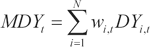
Consequently, the total return of the overall market in month t is:

We use three different weighting factors when constructing our indices. Firstly, we use market capitalization as a weighting factor, where

Secondly, we use a paid-up capital as a weighting factor, where

Thirdly, we use an equally weighted (or unweighted) method:

where N_t is the number of securities existing on the market at time t; q_i,t is the number of issued shares for stock i; and v_i,t is the paid-up capital for stock i at time t.

The advantage of the unweighted returns is they won't be overly affected by large price movements of large firms. On the other hand, the unweighted returns give equal weight to large economically important stocks and relatively small unimportant stocks. A more fundamental problem is that when stocks are illiquid and trade infrequently, this can introduce a significant bias into equally weighted long-term returns. As some stocks in our sample were traded infrequently, we also weight our returns using paid-up capital and market capitalization in order to overcome this potential upward bias. The weights on the paid-up capital returns will possibly be quite dated, as paid-up capital doesn't change often. However, weighting returns by market capitalization overcomes this deficiency.

In order to take account of the effect of changes in paid-up capital, nominal value (i.e., stock splits), or number of issued shares on stock returns, we eliminate stocks which have such changes from our capital appreciation calculations for the month in which the capitalization change occurs, as it is difficult to determine the actual capital appreciation in such circumstances.Footnote ¹⁵

Annual calendar total returns for the overall market are calculated by compounding monthly returns. Annual calendar capital appreciation is also calculated by compounding monthly returns. Annual dividend yield for the overall market is then calculated by subtracting the annual capital appreciation from annual total return.

Our capital appreciation and total return data are converted into indices, with March 1825 being the base month, at which date the indices (I_t) are set to 100. At month t, the index number for each of the returns series (MA_i, MR_i) equals:

SAMPLE CHARACTERISTICS

In the years 1824/25, 127 companies were formed and still in business at the end of 1825, a further 118 were established and

Figure 1

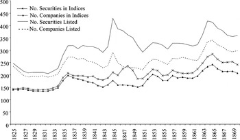
NUMBER OF COMPANIES AND EQUITY SECURITIES IN INDICES AND LISTED IN COURSE OF EXCHANGE AT END OF YEAR, 1825-1870

Notes: The number of securities exceeds the number of companies because firms sometimes had “old” and “new” stock trading simultaneously or firms issued several types of common equity, usually having different paid-up values. For example, from 1837 the National Provincial Bank had two types of common stock: one type had a £100 paid-up value, while the second type had a £20 paid-up value.

subsequently abandoned during the period, and a further 143 companies were projected.Footnote ¹⁶ Although this growth in joint-stock companies may be partially due to the repeal of the Bubble Act and the eradication of corporate monopolies in banking and marine insurance,Footnote ¹⁷ it may also reflect the improved economic conditions due to the Pax Britannica which had emerged following the nation's victory in the Napoleonic wars.

From Figure 1, we can see that the number of companies listed on the Course of the Exchange at the end of 1825 was 236. As can be seen from Figure 1, our sample excludes many of the short-lived “bubble” companies in existence in this period.

The sharp increase in the number of companies in our sample between 1834 and 1836 is predominantly due to the establishment of banks and railways. The increase in the number of railway companies was a result of a boom in railway promotion, whereas the growth in number of joint-stock banks can be largely attributed to the passage of legislation in 1833 (3 & 4 Will. IV, c.98), which permitted non-issuing joint-stock banks to establish in London. The subsequent fall in the number of companies listed and in our index can mainly be explained by the disappearance of companies which had established in the mania of 1836 as well as the demise of ten canal companies.

The famous railway mania of 1844/45 is almost solely responsible for the increase and subsequent fall in the number of securities and companies included in our indices in the mid-1840s. Notably, as can be seen from Figure 1, there were many “bubble” railway companies and securities listed in the Course of the Exchange.

Notably, the freedom to incorporate, which was granted in 1844, and the freedom to incorporate with limited liability, which was granted in 1855, does not appear to have affected the number of companies issuing publicly quoted equity.Footnote ¹⁸ It is only after the passage of the 1862 Companies Act that there is a steep increase in the number of companies listed in the Course of the Exchange and in our sample.Footnote ¹⁹ The financial crisis triggered by the Overend Gurney collapse in May 1866 resulted in the failure of many of these newly established companies, which explains the post-1865 fall in the number of companies listed and in our sample.

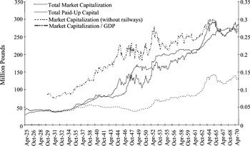
From Figure 2, which contains the paid-up capital and market capitalization of our sample of stocks, we can see that for the decade up until 1834, the value of stocks changed little, which is unsurprising given that the number of companies in our sample doesn't change much in this period. From c.1834 until 1845 nominal total market capitalization and market capitalization as a proportion of GDP increases substantially. As can be seen from Figure 2, this is mostly attributable to the advent of the railways. Notably, it is during the railway mania of the mid-1840s that total paid-up capital and total market capitalization deviate substantially for the first time. The collapse of the railway mania in late 1845 is particularly apparent in the fall in market capitalization as a proportion of GDP. The subsequent calls on railway shareholders to pay up uncalled capital results in an increase in paid-up capital, accompanied by a few years of volatility in the total value of the market.

As can be seen from Figure 2, market capitalization rises quickly from the end of 1851 until July 1853, thereafter it falls markedly over the next ten months. This is more than likely due to the monetary shock arising from the increase in Bank Rate from 3.0 to 5.5 percent over this

Figure 2

MONTHLY MARKET CAPITALIZATION, 1825-1870

Notes: Market Capitalization/GDP is on the right-hand scale. Market Capitalization, Total Paid-Up Capital, and Market Capitalization Without Railways are on the left-hand scale.Sources: See the text.

time period, which was a reaction to harvest failures and the growing threat of war in the Near East.Footnote ²⁰ Indeed, it was only towards the end of the Crimean War that total market capitalization begins to rise again, and it follows an upwards trend (nominally and relative to GDP) until the Overend Gurney collapse in May 1866. A large proportion of the increase in market value, particularly from 1862 onwards, was due to new non-railway companies entering the market.

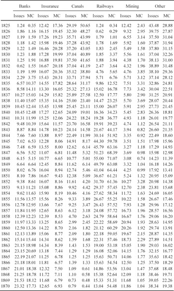
As can be clearly seen from Table 2, great changes occurred in the sectoral composition of the equity market in our sample period. For example, the canal sector dominates our sample in terms of market capitalization and number of issues at the beginning of our sample period, but by the end it has effectively disappeared. On the other hand, from the mid-1830s onwards, railways increasingly dominate our sample in terms of market capitalization and even issues for a time. By the time our sample reaches the 1860s, railways and banks are by far the two largest sectors in terms of market capitalization. In terms of percentage of issues, banks have close to one-fifth of the market in the 1860s, closely followed by the railways.

Table 2

BREAKDOWN OF THE SECTORS CONTAINED IN THE STOCK MARKET INDICES (percentage of issue and market capitalization [mc])

Notes:

The “Other” category includes companies from the following sectors: water utilities; roads; bridges; docks; telegraph companies; gas, light and coke companies; shipping; food production; industrial; brewing; manufacturing; investment, financial and mortgage; and land.

Source:

See the text.

As the Course of the Exchange only covers companies traded on the London market, a question arises as to how representative our sample is of the overall British equity market. Richard Grossman's indices for the British equity market begin in 1870, and his sample covers the majority of equities issued in Britain's various stock exchanges.Footnote ²¹ His sample in 1870 includes 520 equities, with an approximate market capitalization of £750m. In contrast, our sample, which is based on those firms listed on the London stock exchange, has 240 securities with an approximate market capitalization of £285m. The difference in market capitalization is largely explained by the absence of foreign railways from our sample; whereas the difference in issues can be largely attributed to foreign railway stock and joint-stock banks which were traded on the various regional stock exchanges.Footnote ²² Consequently, apart from some Irish, Scottish, and English provincial banks, our sample provides a reasonably good coverage of equity issued by British companies.

INDICES OF CAPITAL APPRECIATION

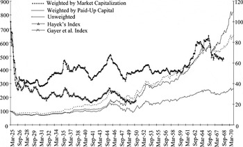
Figure 3 contains our monthly capital appreciation indices. The index weighted by market capitalization outperforms our other indices until early 1867, when the unweighted index surpasses it. This suggests that large companies performed better in terms of capital appreciation than small companies for most of the sample period. However, after early 1867 small firms appear to perform relatively better than large firms, possibly because the risk premia for small firms had increased after the financial crisis stemming from the Overend Gurney crash demonstrated the fragility of small newly formed companies.

Figure 3

MONTHLY INDICES OF CAPITAL APPRECIATION, 1825-1870

Notes: The Gayer et al. index and the Hayek index are on the right-hand scale. Our indices are on the left-hand scale.Sources: See the text and Gayer, Rostow, and Jacobson Schwartz, Growth and Fluctuation, pp. 368-69, 456-57.

The index weighted by paid-up capital performs the least well of the three indices, particularly after the late 1840s. This suggests that companies with larger paid-up capital performed less well than their peers. This is not surprising given that, as can be seen in Figure 2, the paid-up capital of the market exceeded total market capitalization from early 1848 until 1862. A fraction of railway companies which established during the mania had high paid-up capital, but in the crash their share prices fell below their par value and remained there for a long period of time.

As can be seen from Figure 3, the Gayer et al. and Hayek indices differ from our new indices, which is unsurprising given the small samples they used, the method of constructing the indices, and the absence of value weighting. Indeed, our new indices are negatively correlated with that of Gayer et al., and positively correlated with Hayek's.Footnote ²³ This raises the interesting question of whether the indices of Gayer et al. and Hayek allowed them to correctly identify cyclical fluctuations in this period. As we shall see below, Gayer et al.'s hypothesis that rises in share prices were concentrated in major expansion cycles (i.e., 1832-1837 and 1842-1848) isn't always supported by our new indices.Footnote ²⁴

The large fall in the two existing indices at the beginning of the sample period is mainly due to the collapse in mining shares. Our indices also fall at this time, but because of our larger sample, the fall in mining shares has less of an impact on our unweighted index. Indeed, Gayer et al. recognize that a large part of the volatility in their index in the pre-1836 period is due to mining shares. As can be seen from Table 2, mining shares constitute only a small part of our indices at this time, whereas mining stocks constitute approximately 10 percent of the Gayer et al. index.

Like the two existing indices, our indices show a rise in the stock market in 1830, followed by a fall in 1830/31. However, unlike the existing indices, our indices do not show a substantial rise during the 1836 railway mania, followed by a dramatic fall during the commercial crisis of 1837. The reason for this is twofold. Firstly, railways only constitute 17 percent of our weighted indices and less than 14 percent of our unweighted indices at this time, whereas they constitute 44 percent of Gayer et al.'s.Footnote ²⁵ Secondly, the declining canal sector acts as a drag on our indices at this time because they constitute about 27 percent of our indices, whereas they constitute only 16 percent of Gayer et al.'s.

In the period 1837-1841 the increases in our indices suggest rising stock prices, whereas the existing indices suggest falling stock prices. This difference arises for two reasons. Firstly, our indices include the established and newly formed railways, whereas Gayer et al.'s only contains existing railways whose stock fell in this period partly due to the entrance of the new railways.Footnote ²⁶ Secondly, as can be seen from Table 2, railways becoming an increasingly important component of our indices at this time.

The major cycle in the existing indices occurs in the period 1841-1849, a period which is dominated by the railway mania which burst in late 1845. Notably, our indices also display this pattern and move in tandem with the existing indices in this period. Unlike the earlier

Figure 4

MONTHLY DIVIDEND YIELDS FOR ALL INDUSTRIES, 1825-1870

Sources: See the text.

periods, our indices in this period are similar to the existing indices in that the dominant railway sector is roughly given the same weighting. In addition, the railway stock in the existing indices appreciates and depreciates in line with the rest of the railway sector.

Hayek's index is relatively stagnant in the 1850s, whereas the new indices suggest rising stock prices. This difference may simply be down to constituents as our indices include banks and insurance companies, which perform well in this period, whereas Hayek's index doesn't include these sectors. Interestingly, however, our indices correlate closely with Hayek's from about 1860 onwards, suggesting that what Hayek terms industrial shares moved in tandem with the overall equity market.

DIVIDEND YIELDS AND TOTAL RETURNS

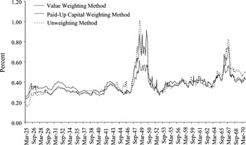
Figure 4, which contains monthly dividend yields for the entire sample, reveals that the dividend yield for the weighted and unweighted series are similar from the 1830s onwards, with the unweighted series being occasionally greater than the weighted series.Footnote ²⁷ This suggests that smaller companies paid similar or higher dividends than their larger counterparts. Economists have traditionally suggested that large (and presumably mature) companies should pay higher dividends as they have fewer investment opportunities.Footnote ²⁸ On the other hand, small companies may be forced to pay higher dividends because of their higher costs of retaining earnings due to agency problems between shareholders and corporate insiders.Footnote ²⁹ An alternative, although less likely, explanation is that the illiquidity of small stocks may have made it prohibitively costly for investors to realize some of their capital gains by selling a proportion of their stock, and, as a result, such firms had to pay higher dividends. Another possible explanation is that companies in early capital markets paid high dividends because reliable information about the true value of stocks was scarce; the lack of information would have been particularly severe for small companies that were trying to attract new investors.Footnote ³⁰

Dividend yields trend slightly upwards over the sample period, although this is less so for the weighted series which contain all companies. However, yields do begin to trend downwards in the late 1860s, and, according to Grossman, this decline continues into the next decade.Footnote ³¹

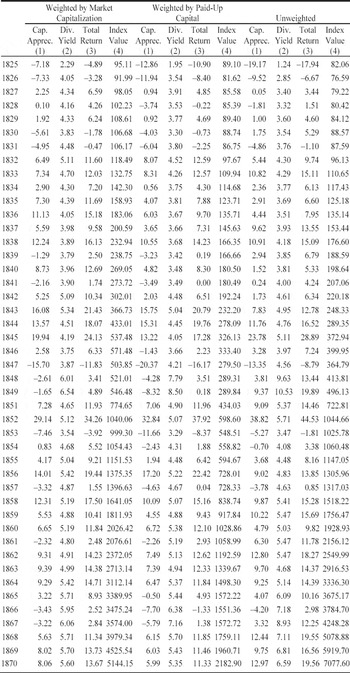
Table 3 contains annual returns as well as the value of the total returns index in December of each year. The extremely high terminal value of the unweighted index reflects the cumulative impact of the higher dividend yields earned by smaller companies. The index weighted by paid-up capital is always below that weighted by market capitalization, thanks to the latter series' higher capital appreciation. As Table 3 shows, the gap between the weighted and unweighted indices widened after 1850, as a result of both higher dividend yields and capital appreciation. After 1850 smaller stocks both paid higher dividends and enjoyed greater capital gains, suggesting that if there was a small-firm effect, it became more apparent from this time onwards. Perhaps the failure of many small railway companies following the railway mania led investors to demand a small-firm premium in this nascent market.

Table 3

ANNUAL STOCK MARKET RETURNS, 1825-1870 (percent)

(1) Capital Appreciation; (2) Dividend Yield; (3) Total Return; (4) Index Value at Dec.

Notes:

Index is total market returns, I_t^MR.

Source:

See the text.

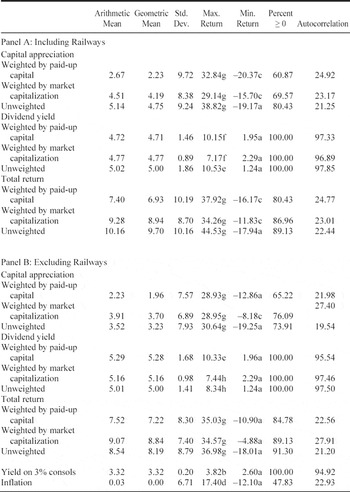
Table 4 contains summary statistics for annualized returns data for the British market in the period 1825-1870. The two panels in the table reveal whether our findings are being driven by railways, the dominant sector in our sample. Several features of these summary statistics in Table 4 are worthy of note. First, shareholders in this era received the majority of their returns through dividends rather than capital gains. Second, the higher returns on the unweighted portfolios of all companies suggest that there is a small-firm premium, although more rigorous analysis is required to prove its existence. Third, railways, the dominant sector in our sample, paid lower dividends than other industries, although the return railroad investors received through capital appreciation was slightly higher. Fourth, the highest total stock market returns in our sample period were achieved in 1852 for both the weighted and unweighted returns, whereas 1825 and 1847 were the worst years. As can be seen from Table 4, the negative returns in 1847 are mainly as a result of the crash of the railway mania. Fifth, although the number of years producing negative capital gains ranges from nine to 18 depending on weighting method, high dividend yields meant that the total stock market return was negative for only six years using the market capitalization weighted returns (1825, 26, 30, 31, 47, and 53). Finally, the relatively high autocorrelation of the capital appreciation series suggests that many stocks were illiquid.

Table 4

SUMMARY STATISTICS FOR ANNUAL STOCK MARKET RETURNS, 1825-1870 (percent)

a = 1825; b = 1826; c = 1847; d = 1848; e = 1849; f =1850; g = 1852; h = 1867.

Note:

Autocorrelation figures for the stock indices are based on monthly return data.

Source:

Inflation data is from O'Donoghue, Goulding, and Allen, “Composite Price Index.”

In order to obtain an estimate of the realized equity risk premium, we use the yield on 3 percent consols as a proxy for the risk-free rate; monthly consol prices were obtained from the Course of the Exchange. consols were widely traded instruments and the efficiency of the market in consols makes them a reliable comparator.Footnote ³² The summary statistics for the yield are reported in Table 4. Comparing our stock market return to this yield suggests that there was a very high equity risk premium in this period. The only other domestic bond finance which investors could hold as alternatives to common equity was railway debentures, but these securities weren't common until the 1860s, and even then they only typically paid 4 percent.Footnote ³³ However, preferred or preference shares were increasingly popular with investors from the late 1840s onwards, and they were widely regarded as a debt-like instrument by investors.Footnote ³⁴ Preference shares were mainly issued by railway companies and paid a fixed income ranging from 4 to 6 percent depending on the individual company, which is substantially less than the returns on common equity reported in Table 4.

Table 4 also shows that average stock returns were much higher than average inflation in this time period. However, our sample period can be neatly subdivided into two subperiods with pre-1850 being a period of deflation and post-1850 being an inflationary period. The arithmetic average nominal and real returns on the portfolio weighted by market capitalization for the pre-1850 period are 8.09 percent and 9.44 percent respectively. The corresponding figures for the post-1850 period are 10.83 percent (nominal) and 10.49 percent (real). Thus, the average returns on the market in the post-1850 period are greater in both nominal and real terms, suggesting that not only did equities outperform general inflation, but that equities performed better in the inflationary environment.

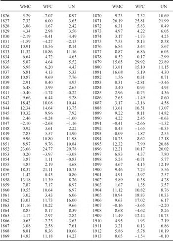
Table 5 presents a series of total returns for the British market for the period 1826-1913. To construct this series, and to ensure compatibility between our series and Grossman's annual series which runs from 1871 to 1913, we used Grossman's method of calculating annual returns. In other words, the annual capital gain for each stock is obtained by comparing December stock prices, and the annual dividend yield is calculated as the annual dividend divided by the previous December's

Table 5

ANNUAL TOTAL RETURNS, 1826-1913 (percent)

Notes:

WPC = weighted by paid-up capital; WMC = weighted by market capitalization; UN = unweighted.

Source:

Returns on British market 1871-1913 are from Grossman, “New Indices.”

stock price. The annual total return was calculated by summing these two components.Footnote ³⁵ As discussed above, our series of returns is a substantial subsample of the companies in Grossman's series, making it feasible to splice these two series.

SURVIVORSHIP BIAS AND RETURNS

As is the case with most stock market indices, our indices are subject to survivorship bias. In other words, stock returns are overestimated because some companies in our sample may have become bankrupt. Typically, one cannot tell from the Course of the Exchange why a particular company was delisted.Footnote ³⁶ Mergers weren't a common reason for delisting in this period, except for railways, and for them Henry G. Lewin gives details of the mergers or name changes which occurred in the decades after the railway mania.Footnote ³⁷ From this list, we identified 53 railways which disappeared from our sample because they merged with another company and three railways which disappeared because of name changes. None of the shares issued by these companies are counted as cases of attrition.

We used three strategies to deal with the remaining companies which disappeared from our sample. The first treats all delisted firms (save, of course, for the merged railroads) as having become bankrupt. The second strategy requires that firms had to be in the market for at least 36 months before they could be considered true victims of attrition; this strategy thus avoids attributing to attrition cases of firms which never fully established in the market.Footnote ³⁸ The third attrition strategy takes into account that some firms delisted for reasons other than bankruptcy. Here we used the Investors' Monthly Manual, which, beginning in the mid-1860s, provides a comprehensive coverage of equity traded on all British markets, not just the London market. We checked the December 1870 edition to see if any of the companies which had at some point disappeared from our sample were still in existence at the end of our sample period. There were 77 firms which had disappeared from our data set but nonetheless appeared in the December 1870 edition of the Investors' Monthly Manual; many of these equities had simply moved their listing to a regional stock exchange. Consequently, these 77 companies are not counted as victims attrition. Note that this third attrition strategy also requires that firms had to be listed for at least 36 months before their subsequence disappearance could be counted as a case of attrition.

Within each attrition strategy, there were two ways we adjusted for survivorship bias. The lower bound adjustment viewed shareholders as suffering a -100 percent return at delisting, and the capital appreciation and dividend yield of the shares were assumed to zero for the rest of our sample period. Information from a stock's last trading month (number of issued shares, price, and paid-up capital) was used to calculate the relevant weighting factor. This could be viewed as a buy-and-hold survivorship bias adjustment. The upper bound adjustment was one which viewed shareholders as suffering a -100 percent return and a zero dividend payment at delisting, with the stock disappearing from their portfolio at this date, which implies that, unlike in the case of our lower bound adjustment, the subsequent zero dividend yields and capital appreciation of delisted stocks do not enter our calculations of average market returns.

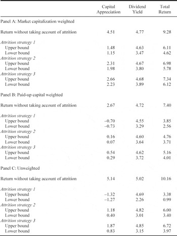
Table 6 reports the attrition-adjusted returns using our three methods. As one can clearly see, the first attrition strategy has the largest effect on our return estimates and the third strategy has the least severe impact. We also observe that attrition reduces the returns of the unweighted portfolios more than those of the weighted portfolios. This suggests that many of our delisting companies are small firms, which is not surprising given their higher probability of bankruptcy. Notably, the lower bound attrition method has a greater impact, relatively speaking, on capital appreciation.

After accounting for attrition using the lower bound method, one can see from Table 6 that dividends now constitute a greater proportion of total return. Indeed, apart from the market capitalization weighted returns, annual capital appreciation is very close to zero. This suggests that shareholders enjoyed capital appreciation mainly on stocks of large firms. Interestingly, after taking account of attrition using the upper bound adjustment, the unweighted dividend yields are still larger than the weighted returns, suggesting that smaller stocks have higher dividend yields.

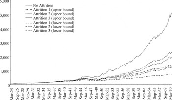
Figure 5 plots indices of total returns weighted by market capitalization. One can see that over the sample period, attrition has a substantial impact on the total return indices. Nevertheless, even using the estimate from the most severe attrition methodology, investors still enjoy a substantial return over this time period as the total return index grows 741 percent by 1870, with the annual rate of return being 4.62 percent.

Table 6

AVERAGE ANNUAL STOCK MARKET RETURNS AFTER ATTRITION ADJUSTMENTS, 1825-1870 (percent)

Notes:

The three attrition strategies compensate for survivorship bias. For the definition of each, see the text.

Source:

See the text.

Figure 5

MONTHLY INDICES OF TOTAL RETURN WEIGHTED BY MARKET CAPITALIZATION, 1825-1870

Notes: See the text for the definitions of these various attrition measures.Sources: See the text.

One potential weakness with our correction for survivorship bias is that it ignores the losses produced by companies (particularly fraudulent ones) that briefly entered but were listed for less than 12 months before disappearing. Investors may have lost significant sums to such companies, particularly during the railway mania of the mid-1840s, when there were a number of “bubble” or fraudulent promotions. Omitting these companies, however, is unlikely to bias our results significantly, for at least three reasons. First, the companies were typically small entities, and therefore would have little impact on our weighted series of returns. Second, many of the companies which delisted within 12 months did so because there were unable to attract sufficient funds from investors. Third, investors who did put money in short-lived companies typically only paid in a very small amount of capital initially; that was true in particular of railways.Footnote ³⁹ Further calls were only issued if the company was successful in getting off the ground. Hence, investors in short-lived companies typically lost very little.

THE COMPARATIVE PERFORMANCE OF THE 1825-1870 EQUITY MARKET

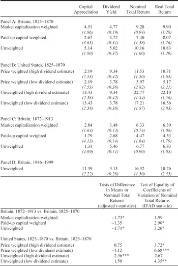
Table 7 compares the returns on the British equity market in the 1825-1870 period with those of the United States in the same period and with later epochs in the British market. Although such comparisons help place the performance of the 1825-1870 British equity market in context, they should be made circumspectly due to possible differences in construction, constituents, and survivorship bias.

Richard Sylla, in his recent comparison of the British and U.S. financial systems, suggests that by 1830 the U.S. financial system had more corporations (due to liberal incorporation laws) and a better developed securities market.Footnote ⁴⁰ However, he also suggests that the U.S. financial system went into a reversal over the subsequent four decades, allowing the British financial system to catch up with its U.S. counterpart. Consequently, a comparison of the performance of these two equity markets in this period should prove instructive for his thesis. Comparing the unweighted returns for Britain with those for the United States, it is noteworthy that the real return estimates for the United States are higher than those of Britain, although the difference in means between the British unweighted return and the low-dividend estimate for the United States is not statistically significant. However, as the higher coefficient of variation shows, the U.S. market was riskier than the British market. Alternatively, the high capital appreciation for the United States could be due to the upward bias induced by the large movements of stock prices which sometimes arise as a consequence of infrequent trading.Footnote ⁴¹ As price or capitalization weighted returns to a large extent eliminate this bias, it may be more illuminating to compare the weighted returns for the United States and Britain. If we do so, we find that the differences in average annual real returns are not statistically significant from zero. That is somewhat surprising given the higher levels of risk in the United States market as measured by the coefficient of variation. Notably, in both markets, dividend returns are the major component of total returns, which is the reverse of what we observe in modern equity markets.Footnote ⁴²

As we can see from Panels C and D of Table 7, total real returns are lower in both the 1872-1913 and 1946-1999 periods than in the period 1825-1870. One possible explanation for this is that the market

Table 7

COMPARISON OF ANNUAL AVERAGE RETURNS WITH UNITED STATES AND POST-1870 BRITAIN (percent)

* denotes significance at the 10 percent level.

** denotes significance at the 5 percent level.

*** denotes significance at the 1 percent level.

Notes:

Coefficient of variation is in parenthesis. Market capitalization weighted stock returns is used to proxy the price weighted returns for Britain over 1825 to 1870. The t-values are adjusted to account for the serial correlation of stock returns. The adjusted t-statistic takes the form:

where α is the first-order autocorrelation of the sample returns, s is the sample standard deviation, and n is sample size. The D'AD statistic is from Feltz and Miller, “Asymptotic Test,” and is a test of the equality of coefficients of variation and is asymptotically chi-squared.

Source:

Returns on British market 1872-1913 and 1946-1999 are from Grossman, “New Indices.” Returns on U.S. market are calculated from data reported in Goetzmann, Ibbotson, and Peng, “New Historical Database.” Inflation data to calculate real returns was obtained from O'Donoghue, Goulding, and Allen, “Composite Price Index,” for Britain and Officer and Williamson, “Annual Inflation Rates,” for the United States.

was less risky in the post-1870 period, but a comparison of the coefficients of variation suggests that the pre-1870 and post-1870 eras were just as risky if not riskier. This appears somewhat paradoxical given that uncalled capital was a common feature of many companies up until the 1870s.Footnote ⁴³ Indeed, many banks and insurance companies had unlimited liability, which can be viewed as an extreme form of uncalled capital callable only in the event that the firm enters bankruptcy. However, the existence of uncalled capital may have acted as a substantial check on management risk-taking behavior, reducing the riskiness of stocks carrying uncalled capital. Uncalled capital was less prevalent in the British equity market after the 1870s, and therefore the check on managerial risk-taking behavior was removed in some cases.Footnote ⁴⁴