





1. Introduction
When sequences of outcomes are generated by random mechanisms such as coin tosses or roulette spins, some people may incorrectly believe that a particular outcome is less likely if it has recently occurred with higher-than-expected frequency. For example, if a roulette ball has landed on red several times in a row, some people may believe that black is more likely on the next spin. This error is the gambler’s fallacy. It has been documented in a variety of settings, including among bettors in casinos (Croson and Sundali, Reference Croson and Sundali2005; Sundali and Croson, Reference Sundali and Croson2006), lotteries (Coltfelter and Cook, Reference Coltfelter and Cook1993; Suetens and Tyran, Reference Suetens and Tyran2012; Terrell, Reference Terrell1994), and sports markets (Durham et al., Reference Durham, Hertzel and Martin2005); among investors (Loh and Warachka, Reference Loh and Warachka2012; Pelster, Reference Pelster2020), couples considering whether to have another child (McClelland and Hackenberg, Reference McClelland and Hackenberg1978), and goal keepers in high-stakes football (soccer) matches (Misirlisoy and Haggard, Reference Misirlisoy and Haggard2014); and among baseball umpires, loan officers, and asylum judges (Chen et al., Reference Chen, Moskowitz and Shue2016).Footnote 1
1.1. The role of probabilistic reasoning
Explanations of the gambler’s fallacy are typically based on people’s perceptions of randomness. Such perceptions have been studied in numerous ways, including having participants judge the randomness of sequences (e.g., Scholl and Greifeneder, Reference Scholl and Greifeneder2011), having them distinguish between random and nonrandom sequences (e.g., Lopes and Oden, Reference Lopes and Oden1987), having them attempt to generate random sequences (e.g., Rapoport and Budescu, Reference Rapoport and Budescu1997), and having them make predictions or likelihood judgments regarding the next outcome in a sequence (e.g., Jarvik, Reference Jarvik1951). We reserve the term gambler’s fallacy for the latter variety of task, but the relevant theories often address perceptions of randomness more generally.
Kahneman and Tversky’s (Reference Kahneman and Tversky1972) representativeness heuristic is by far the most commonly invoked account of perceived randomness and the gambler’s fallacy. According to the heuristic, people believe that observed sequences should have properties that reflect the salient features of the generating process. For a random process (e.g., flipping a coin), belief in local representativeness (or similarly, belief in the so-called law of small numbers; Tversky and Kahneman, Reference Tversky and Kahneman1971) implies that even short sequences should look random. Evidence indicates that ‘looking random’ entails an observed proportion of outcomes that is close to the base rate (e.g., 50% for coin flips), an excess of alternations (e.g., heads followed by tails), and an absence of long streaks (e.g., five heads in a row) (Kahneman and Tversky, Reference Kahneman and Tversky1972; Oskarsson et al., Reference Oskarsson, Van Boven, McClelland and Hastie2009; Rao and Hastie, Reference Rao and Hastie2023). These features (and others such as complexity, which is related to the lack of shortcuts for describing a sequence and thus to participants’ difficulty in memorizing or copying the sequence; Falk and Konold, Reference Falk and Konold1997) are not independent: A streak of five heads is associated with a deviation from the base rate and a lower-than-expected alternation rate, at least over the short run. If the generating process is believed to be random, these departures from expectations can lead to the incorrect belief that a reversal is in order (i.e., the gambler’s fallacy).
Quantitative theories in the heuristics and biases tradition incorporate inaccurate perceptions of randomness as a central feature. For example, Rapoport and Budescu’s (Reference Rapoport and Budescu1997) model for sequence generation assumes a belief that sequences should be locally representative in terms of outcome proportions, Rabin’s (Reference Rabin2002) model for outcome prediction assumes a belief that outcomes are generated by sampling without replacement from an ‘urn’ of limited capacity (even when outcomes are independent), and Rabin and Vayanos’s (Reference Rabin and Vayanos2010) model for outcome prediction assumes a belief that random sequences alternate more than they really do.
Critics of the heuristics and biases approach have pointed out that perceptions of randomness do not appear so inaccurate when judged against the characteristics of sequences people actually experience (Farmer et al., Reference Farmer, Warren and Hahn2017; Hahn and Warren, Reference Hahn and Warren2009; Kareev, Reference Kareev1992). For example, while the strings HHHT and HHHH would (theoretically) occur equally often in an infinite series of coin flips, their chances of occurring at least once in a sequence of 20 flips are about 75% and 48%, respectively; on average, it takes substantially fewer flips to observe HHHT than to observe HHHH (Hahn and Warren, Reference Hahn and Warren2009).Footnote 2 In this experiential sense, it does not seem so wrong to think that a streak of four heads is less common. Such experiences suggest alternative benchmarks for assessing perceptions of randomness. These benchmarks can be used normatively, as the correct answer in certain tasks (e.g., is HHHT or HHHH more likely to occur first in a series of coin flips?), or descriptively, to predict people’s responses in such tasks. However, for three tasks in which alternative benchmarks provided the normatively correct answer, Reimers et al. (Reference Reimers, Donkin and Le Pelley2018) reported that measures of the representativeness of outcome proportions, alternation rates, and sequence complexity outperformed the alternative norms in predicting participants’ responses.
A recent Bayesian updating model from Dorst (Reference Dorst2026) is based on an entirely different premise. Because people have experience with many sequences that are either ‘switchy’, ‘steady’, or ‘sticky’ (i.e., sequences with negative, zero, or positive sequential dependencies, respectively), a person’s prediction about the next outcome reflects their probabilistic beliefs about the type of sequence they are dealing with. In this model, the gambler’s fallacy occurs because sequences from a statistically independent process rule out the ‘sticky’ hypothesis faster than they rule out the ‘switchy’ hypothesis.
This brief overview highlights the importance of probabilistic reasoning in accounting for the gambler’s fallacy. All the above theories involve some form of probabilistic reasoning, but not all assume that a person develops a subjective probability judgment regarding the next outcome. For example, in Rapoport and Budescu’s (Reference Rapoport and Budescu1997) model for sequence generation, a person considers the last several outcomes and chooses as the next outcome the one that maximizes the local representativeness of the augmented sequence.
1.2. Xiang et al.’s (Reference Xiang, Dorst and Gershman2025) article
Against this backdrop, Xiang et al. (Reference Xiang, Dorst and Gershman2025; hereafter XDG) raised two important issues. First, they noted that most studies of the gambler’s fallacy have involved binary predictions or choices rather than probability judgments.Footnote 3 Reliance on binary predictions is natural and perhaps unavoidable in field studies (Chen et al., Reference Chen, Moskowitz and Shue2016; Coltfelter and Cook, Reference Coltfelter and Cook1993; Croson and Sundali, Reference Croson and Sundali2005; Durham et al., Reference Durham, Hertzel and Martin2005; Misirlisoy and Haggard, Reference Misirlisoy and Haggard2014; Pelster, Reference Pelster2020; Suetens and Tyran, Reference Suetens and Tyran2012; Sundali and Croson, Reference Sundali and Croson2006; Terrell, Reference Terrell1994), but there is no such restriction in the lab or in surveys, where binary predictions have also been the norm (Altmann and Burns, Reference Altmann and Burns2005; Ayton and Fischer, Reference Ayton and Fischer2004; Barron and Leider, Reference Barron and Leider2010; Choi et al., Reference Choi, Kim and Son2025; Jarvik, Reference Jarvik1951; Roney and Sansone, Reference Roney and Sansone2014; Roney and Trick, Reference Roney and Trick2003; Stöckl et al., Reference Stöckl, Huber, Kirchler and Lindner2015). XDG’s issue with such studies is that they do not provide direct evidence regarding the probabilistic reasoning processes on which most theories of the fallacy are based. We agree with XDG that assessing both probability judgments and binary predictions is important for theory testing.
The second issue raised by XDG was that, while some lab and survey studies have elicited probability judgments (Burns and Corpus, Reference Burns and Corpus2004; Dohmen et al., Reference Dohmen, Falk, Huffman, Marklein and Sunde2009; Matarazzo et al., Reference Matarazzo, Carpentieri, Greco and Pizzini2019; Navarrete and Santamaría, Reference Navarrete and Santamaría2012; Rao and Hastie, Reference Rao and Hastie2023), most have done so only for nonrandom, intentionally constructed sequences rather than random sequences (exceptions include Asparouhova et al., Reference Asparouhova, Hertzel and Lemmon2009; Benjamin et al., Reference Benjamin, Moore and Rabin2017; de Lara, Reference de Lara2026). Although XDG did not label it as such, this is an issue of representative versus experimental design (Dhami et al., Reference Dhami, Hertwig and Hoffrage2004; Hammond and Stewart, Reference Hammond and Stewart2001). A central goal of representative design is to preserve the important features of real-world stimuli (e.g., distributions and correlations) so that participants’ thought processes—and thus researchers’ conclusions—are not affected by unrealistic stimulus sets. The downside is that representative designs are often statistically inefficient, making tests of theoretically relevant relationships such as linear or quadratic effects or interactions between predictors less powerful (McClelland and Judd, Reference McClelland and Judd1993; McClelland, Reference McClelland1997). In the context of the gambler’s fallacy, sets of randomly generated sequences are representative, but theoretically interesting sequences with long terminal streaks are very rare. Nonetheless, we agree with XDG that it is important to assess whether a gambler’s fallacy exists for probability judgments when random sequences are used.
As described in detail below, XDG conducted a series of five studies to address their two concerns. For random sequences, they reported a significant gambler’s fallacy for binary predictions but not for probability judgments. Moreover, two models for predicting participants’ binary responses on the basis of other participants’ probability judgments performed poorly, and a third model based on the representativeness heuristic did not predict either set of responses. Noting the apparent disconnection between results for probability judgments and binary responses, XDG suggested a need for new theories that do not rely on probabilistic reasoning.
1.3. The current reanalysis
We disagree with some of XDG’s conclusions and with the implications for theories of the gambler’s fallacy. The problem is not that XDG’s analyses were incorrect, but rather that their analyses were insufficiently thorough and overly selective. For example, their primary statistical analyses relied heavily on aggregating responses over terminal streak lengths (thereby downplaying this theoretically relevant moderator) while not aggregating over base rates, even when the data were from the same participants (thereby reducing statistical power). Of particular concern, XDG did not assess the predictive ability of any published model of the gambler’s fallacy, relying instead on an inadequate implementation of the representativeness heuristic.
For the current article, we used XDG’s statistical procedures and very similar procedures to reexamine their evidence regarding a gambler’s fallacy for probability judgments and the relationship between probability judgments and binary predictions. Our decision to use procedures like XDG’s was mostly strategic. Using very different procedures would run the risk of ‘they said, we said’ conclusions that would leave readers in a position of evaluating the relative merits of competing methodological claims. Using similar procedures—but pursuing them more thoroughly—keeps the focus on the data and the substantive conclusions. Moving beyond XDG’s analyses, we also assessed the potential of probabilistic models to account for both probability judgments and binary predictions by examining an improved specification of XDG’s representativeness model and a version of Rabin and Vayanos’s (Reference Rabin and Vayanos2010) highly regarded model for the gambler’s and hot-hand fallacies.
To foreshadow our results, we found strong evidence for a gambler’s fallacy for probability judgments, although there was substantial heterogeneity across participants. We also found a stronger relationship between probability judgments and binary predictions than XDG indicated. Finally, our revised representativeness model and our implementation of the Rabin–Vayanos model accounted for both measures reasonably well, suggesting that XDG’s most sweeping conclusions (e.g., that ‘[binary] prediction does not rely on probabilistic reasoning’, p. 642) were unsubstantiated. We conclude with suggestions for more efficient random-sampling schemes that guarantee representative sequences for every participant.
2. Xiang et al.’s ( Reference Xiang, Dorst and Gershman2025) experiments and results
For readers unfamiliar with XDG’s experiments and primary results, we review the details below.
2.1. XDG’s five experiments
XDG conducted a series of five online experiments, each with 150 participants, based on Rao and Hastie’s (Reference Rao and Hastie2023) bingo-ball color-prediction task. On each trial of each experiment, participants viewed a sequence of eight balls, one after another, drawn from a covered mechanical bingo cage. Participants were told that after each ball, the ball would be rolled back into the cage, which would be spun again before the next ball was drawn (i.e., that sampling was with replacement). After seeing the sequence of eight balls (which remained visible on the screen), participants predicted the color of the ninth ball. There were 18 such trials in each experiment.
In Experiments 1a and 1b, the cage was said to contain 50 blue balls and 50 red balls. The color of each ball for each participant was determined independently by sampling from a Bernoulli distribution with p = .5. Participants in Experiment 1a answered the question, ‘What is the probability that the next ball drawn from the cage will be RED?’ by clicking a slider bar and adjusting the slider to the desired position. The endpoints of the slider bar were labeled 0% and 100%, but there were no markings or labels between those points. Participants in Experiment 1b answered the question, ‘What color bingo ball will the machine draw next? Will it be BLUE or RED?’ by clicking one of two buttons.
Experiments 2a and 2b were the same as Experiments 1a and 1b, respectively, except that the bingo cage was said to contain either 60 blue balls and 40 red balls or 40 blue balls and 60 red balls. The mix was randomized for each participant in each experiment and remained the same for all 18 trials. For data analysis, XDG divided trials into those in which the eighth ball had a base rate of 60% (regardless of its color) and those in which the eighth ball had a base rate of 40%. Thus, the data for the 60% and 40% base rates were from the same participants in each experiment.
Experiment 3 was the same as Experiment 1a in that it involved a 50% base rate and probability judgments, but the colors of the balls in each sequence were not determined randomly. Instead, the sequences were identical to those in the bingo condition of Rao and Hastie’s (Reference Rao and Hastie2023) Experiment 2A, which XDG’s Experiment 3 was designed to replicate. Specifically, 12 of the 18 sequences ended with a terminal ‘streak’ of one ball (i.e., each ended with a reversal, blue-red or red-blue), and the remaining six sequences ended with terminal streaks of two to seven balls (one sequence of each type). For each participant, sequences were drawn from larger pools of similar sequences. The presentation order was randomized, but the first sequence always had a terminal streak length of one (see Rao and Hastie’s, Reference Rao and Hastie2023, Supplementary Material for details).
2.2. XDG’s primary results
2.2.1. Means and medians for probability judgments
XDG’s participants made probability judgments in Experiments 1a, 2a, and 3. To facilitate comparisons between base rates and (later) aggregation over base rates, we first subtracted the relevant base rate from each probability judgment; negative deviations are consistent with the gambler’s fallacy. Following XDG, we averaged responses over sequences for each participant.
XDG’s results for random sequences with different base rates appear in the first three rows of Table 1 (excluding the last column). For the 50% and 40% base rates, the Wilcoxon tests indicated that the sample medians were not significantly different from zero (i.e., the median probability judgments were not significantly different from the base rate). The Bayesian 95% credible intervals for the effect sizes included zero, indicating that the evidence was consistent with the absence of the gambler’s fallacy. The Bayes factors indicate whether the data were more likely to have come from the alternative hypothesis (
${BF}_{10}>1$
 ) or the null hypothesis (
${BF}_{10}<1$
 ). For XDG’s Bayes factors (from the R package BayesFactor; Morey and Rouder, Reference Morey and Rouder2024), the prior distribution for the effect size under the alternative hypothesis was a weakly informative Cauchy distribution centered at zero and with half the effect sizes beyond ±0.707 (i.e., a symmetric, thick-tailed distribution), while the prior distribution under the null hypothesis was a spike at zero. For the 50% and 40% base rates, the Bayes factors indicated ‘moderate’ evidence in favor of the null hypothesis (for interpreting Bayes factors, we use the scale from Wagenmakers et al., Reference Wagenmakers, Love, Marsman, Jamil, Ly, Verhagen, Selker, Gronau, Dropmann, Boutin, Meerhoff, Knight, Raj, van Kesteren, van Doorn, Šmíra, Epskamp, Etz, Matzke and Morey2018). However, for the 60% base rate, the Wilcoxon test indicated a significant gambler’s fallacy, the 95% credible interval excluded zero, and the Bayes factor indicated ‘extreme’ evidence in favor of the alternative hypothesis. Consequently, XDG’s statement that their conclusions for the 50% base rate ‘appear to hold rather broadly’ (p. 460) seems unjustified to us.
Probability judgments for repetition of the terminal outcome (relative to the base rate), one-sample Wilcoxon signed-rank tests, Bayesian t tests, and replication Bayes factors

Table 1. Long description
The table is divided into two primary sections.
Section 1: All terminal streak lengths.
Under Random sequences:
- Experiment 1a (Base rate 50): Mean -0.67, Median 0.00, z -1.03, B F sub 1 0 0.25.
- Experiment 2a (Base rate 40): Mean -0.96, Median -1.69, z -1.77, B F sub 1 0 0.15.
- Experiment 2a (Base rate 60): Mean -4.53, Median -1.75, z -3.65, B F sub 1 0 421.92.
- Experiment 2a (Base rate 40, 60): Mean -3.04, Median -1.36, z -4.45, B F sub 1 0 greater than 10 super 3.
- Experiments 1a and 2a combined: Mean -1.85, Median -0.50, z -4.17, B F sub 1 0 973.31.
Under Nonrandom sequences:
- Experiment 3: Mean -1.78, Median -0.33, z -4.02, B F sub 1 0 273.61.
- R H 2A: Mean -2.47, Median -0.86, z -2.50, B F sub 1 0 3.91.
Section 2: Terminal streak lengths greater than 1.
Under Random sequences:
- Experiment 1a: Mean -1.70, Median -0.45, z -2.21, B F sub 1 0 0.76.
- Experiment 2a (Base rate 40): Mean -5.42, Median -5.00, z -4.22, B F sub 1 0 100.36.
- Experiment 2a (Base rate 60): Mean -6.77, Median -2.55, z -4.19, B F sub 1 0 greater than 10 super 4.
- Experiment 2a (Base rate 40, 60): Mean -6.21, Median -2.24, z -5.15, B F sub 1 0 greater than 10 super 5.
- Experiments 1a and 2a combined: Mean -3.95, Median -1.10, z -5.31, B F sub 1 0 greater than 10 super 5.
Under Nonrandom sequences:
- Experiment 3: Mean -3.21, Median -0.50, z -2.32, B F sub 1 0 1.16.
- R H 2A: Mean -5.79, Median -5.17, z -2.30, B F sub 1 0 2.30.
Negative values indicate consistency with the gambler's fallacy. B F sub 1 0 represents the Bayes factor in favor of the alternative hypothesis.
Note: Probability judgments are for the repetition of the terminal outcome, relative to the base rate; negative values are consistent with the gambler’s fallacy.
${BF}_{10}$
 = Bayes factor in favor of the alternative hypothesis relative to the null hypothesis. Values of 1–3 = ‘anecdotal’ evidence, 3–10 = ‘moderate’ evidence, and above 100 = ‘extreme’ evidence (Wagenmakers et al., Reference Wagenmakers, Love, Marsman, Jamil, Ly, Verhagen, Selker, Gronau, Dropmann, Boutin, Meerhoff, Knight, Raj, van Kesteren, van Doorn, Šmíra, Epskamp, Etz, Matzke and Morey2018).
$1/{BF}_{10}$
 yields a Bayes factor in favor of the null hypothesis. RH = Rao and Hastie (Reference Rao and Hastie2023). N = 150 participants except in Experiments 1a and 2a combined (N = 300) and Rao and Hastie’s (Reference Rao and Hastie2023) Experiment 2A (N = 56).
† p < .10;\ *p < .05; *** p < .001.
As can be seen in the sixth row of Table 1, XDG’s Experiment 3, which used a 50% base rate and nonrandom sequences, yielded a reliable gambler’s fallacy, with the Bayes factor indicating ‘extreme’ evidence in that direction. A Wilcoxon rank-sum test indicated that the medians in Experiments 1a (with random sequences) and 3 (with nonrandom sequences) were significantly different (p = .025). This comparison constituted XDG’s primary evidence that random and nonrandom sequences lead to different results.
2.2.2. Effects of terminal streak length
XDG also reported results separately for each base rate and terminal streak length (see Figure 1, which is adapted from XDG’s Figure 5; ignore the model predictions for now). For these analyses, XDG first averaged probability judgments (or binary predictions) over sequences with the same terminal streak length for each participant. They then computed the means and medians across participants at each streak length (i.e., means and medians of participants’ means), along with bootstrapped 95% confidence intervals. The most salient feature of the data in the figure is that the gambler’s fallacy is more evident for binary predictions than for probability judgments. There is also the appearance of nonlinearity, perhaps more obvious for binary predictions than for probability judgments, with responses first decreasing as a function of terminal streak length and then leveling out or increasing at longer streak lengths (we caution that there was much less data at longer streak lengths, especially for the 40% base rate). XDG assessed the nonlinearity with Bayesian mixed-effects regressions for the binary predictions in Experiment 1b (the 95% credible interval for the quadratic effect excluded zero) and for the probability judgments in Experiment 3 (the credible interval included zero; see their Table 1), but not for the probability judgments in Experiments 1a and 2a, which are of principal interest here.
(a) Mean and median probability judgments that a streak will continue for different terminal streak lengths and base rates, with predictions from one of XDG’s models and two models not considered by XDG. (b) Mean proportions of binary predictions that a streak will continue, with predictions from three of XDG’s models. (c) Mean proportions of binary predictions that a streak will continue, with predictions from two models not considered by XDG. Dashed lines indicate base rates. Error bars indicate bootstrapped 95% confidence intervals. For the 40% base rate (bottom row), the points for streak lengths 6, 7, and 8 represent 6, 2, and 3 participants (respectively) for probability judgments and 3, 2, and 3 participants for binary predictions. All other points represent at least 15 participants. Source: Adapted from Xiang et al. (2025, p. 457). Copyright 2025 by the authors. Adapted with permission.

Figure 1. Long description
The figure consists of nine line graphs arranged in three columns and three rows.
Column a, titled Probability Judgments, shows the Probability of Streak Repeating percentage on the y-axis. Column b and c, both titled Binary Predictions, show the Proportion Predicting Streak Will Repeat percentage on the y-axis.
The rows are categorized by base rates indicated in grey vertical bars on the right: the top row is 50 percent, the middle row is 60 percent, and the bottom row is 40 percent. The x-axis for all graphs is Terminal Streak Length ranging from 1 to 8.
In Column a, the Mean of Participants’ Means is shown as light blue circles with error bars. It is compared against X D G's Representativeness Model (green squares), Revised Representativeness Model (dark blue squares), and Rabin and Vayanos's Model (pink triangles). Generally, the green model shows a steep decline as streak length increases, while the blue and pink models show a more gradual decline.
In Column b, the participant mean is compared against three X D G models: Thresholding Model (yellow diamonds), Subjective Model (orange triangles), and Representativeness Model (green squares). The Subjective and Thresholding models tend to stay closer to the participant data, which fluctuates more than the probability judgments.
In Column c, the participant mean is compared against the Revised Representativeness Model (dark blue squares) and Rabin and Vayanos's Model (pink triangles).
Horizontal dashed lines in each graph represent the respective base rate. Error bars represent bootstrapped 95 percent confidence intervals. In the 40 percent base rate row, participant data points for streak lengths 6, 7, and 8 have significantly larger error bars due to smaller sample sizes.
2.2.3. The disconnection between probability judgments and binary predictions
XDG provided two lines of evidence suggesting a disconnection between probability judgments and binary predictions. The first was that the results for the two tasks did not seem to line up: In Figure 1, the gambler’s fallacy appears much larger for binary predictions for all three base rates. Interestingly, the Wilcoxon tests and Bayes factors for binary predictions indicated a gambler’s fallacy for the 50% and 40% base rates (both ps < .001, both
${BF}_{10}$
 s > 1,000), but not for the 60% base rate (p = .341,
${BF}_{10}$
 = 0.149).Footnote
4
These results were essentially the opposite of those for probability judgments.
Second, XDG could not reconstruct the binary predictions in Experiments 1b and 2b from the probability judgments in Experiments 1a and 2a using either a thresholding model or a subjective probability model. In both models, a participant’s probability judgment was used to make a predicted binary response, and these predictions were averaged for each combination of base rate and terminal streak length. XDG’s thresholding model predicted continuation of the streak if the probability judgment was above the base rate and reversal of the streak if the probability judgment was below the base rate. If the probability judgment equaled the base rate (which could happen only for the 50% base rate), the binary prediction was determined randomly. XDG’s subjective probability model converted probability judgments to binary predictions according to a sequential-sampling process (Zhu et al., Reference Zhu, Sundh, Spicer, Chater and Sanborn2024) in which outcomes were drawn from a Bernoulli distribution based on the reported probability until one outcome outnumbered the other by a specific margin k (XDG used k = 5, but they also reported results for margins of 2, 10, and 20 in their Supplementary Material; when the probability is not .5, predicted proportions become more extreme with larger values of k).Footnote 5 As is evident in the middle column of Figure 1, these models were relatively poor at predicting participants’ binary responses.
Taking the disconnection as given, XDG evaluated the ability of a representativeness model to explain the gap between probability judgments in Experiments 1a and 2a and binary responses in Experiments 1b and 2b. Rather than using one set of judgments to predict the other, this approach allowed the two sets of judgments to share a common source. The model, which was based on the discrepancy between the observed proportion of outcomes in a sequence and the underlying base rate, made inaccurate but similar predictions in the two tasks (see the left and center columns in Figure 1), suggesting to XDG that ‘the representativeness heuristic alone cannot explain the two judgments’ (p. 462). However, as we explain later, the model had a number of serious problems that made it a poor tool for assessing the explanatory power of the representativeness heuristic.
3. Reanalysis of Xiang et al.’s ( Reference Xiang, Dorst and Gershman2025) data
Although other approaches are possible, we wanted to assess whether XDG’s conclusions would withstand a closer look with their methods and minor extensions of those methods.
3.1. Aggregation over base rates
We repeated XDG’s Wilcoxon tests and Bayesian t tests (their main analyses) after combining the data for the 40% and 60% base rates in Experiment 2a (the data were from the same participants) and after combining the data from Experiments 1a (50%) and 2a (40% and 60%). For Experiment 2a, computing a single mean probability per participant yielded a significant gambler’s fallacy (p < .001) and a Bayes factor of over 1,000 (see Table 1). For Experiments 1a and 2a combined, the gambler’s fallacy was again significant (p < .001), and the Bayes factor was nearly 1,000.
In addition, we used XDG’s procedures to compute bootstrapped 95% confidence intervals for mean and median probability judgments at each terminal streak length, as in the left column of Figure 1 but for all three base rates combined. The results appear in Figure 2. The confidence intervals for mean probability judgments indicated a significant gambler’s fallacy for streak lengths 2, 3, 4, 5, and 7. For median judgments, the confidence intervals excluded zero for streak lengths 3, 4, and 7; for streak lengths 2 and 5, the upper limit of the confidence interval was zero. When the terminal streak length was four, the mean was −7.17 pp (95% CI [−9.72, −4.69]), and the median was −3.00 pp (95% CI [−6.00, −1.00]). XDG’s bold conclusion regarding the absence of a gambler’s fallacy for probability judgments when sequences are random does not withstand aggregation of their data over base rates.
Mean and median probability judgments (deviations from the base rate, in percentage points) at each streak length when data are aggregated over Experiments 1a (50% base rate) and 2a (40% and 60% base rates). Error bars indicate bootstrapped 95% confidence intervals.

Figure 2. Long description
The x-axis is labeled Terminal Streak Length with integer increments from 1 to 8. The y-axis is labeled Probability of Streak Repeating (Deviation from Base Rate in p p) ranging from negative 30 to 10. A horizontal dashed line marks the 0 deviation point.
Two data series are plotted:
* Mean (of Participants’ Means) represented by light blue circles.
* Median (of Participants’ Means) represented by dark blue triangles.
Both series start near 0 at streak length 1. As streak length increases to 4, both lines show a downward trend, with the mean reaching approximately negative 7 and the median reaching approximately negative 3. At streak length 5 and 6, there is a slight recovery toward 0. At streak length 7, both values drop sharply to their lowest point near negative 14. At streak length 8, the mean rises to negative 5 while the median returns to 0. Vertical error bars representing confidence intervals are present for each point, becoming significantly larger at streak lengths 7 and 8.
3.2. Sequences with terminal streak lengths greater than one
About half of XDG’s sequences had terminal streak lengths of one, but the gambler’s fallacy is often absent or reversed for such sequences (Altmann and Burns, Reference Altmann and Burns2005; Asparouhova et al., Reference Asparouhova, Hertzel and Lemmon2009; Ayton and Fischer, Reference Ayton and Fischer2004; Barron and Leider, Reference Barron and Leider2010; Croson and Sundali, Reference Croson and Sundali2005; Jarvik, Reference Jarvik1951; Stöckl et al., Reference Stöckl, Huber, Kirchler and Lindner2015). This is perhaps because the terminal outcome is viewed as ending a previous streak (Roney and Sansone, Reference Roney and Sansone2014) or because ‘streaks’ of length one are not considered streaks at all (Carlson and Shu, Reference Carlson and Shu2007). Unlike XDG, Rao and Hastie (Reference Rao and Hastie2023) treated such sequences as ‘fillers’ and excluded them from their primary analyses.
We repeated XDG’s Wilcoxon tests and Bayesian t tests for sequences in which the terminal streak length was greater than one. The results appear in the bottom half of Table 1. The means and medians are all more negative than in the top half of the table, indicating stronger tendencies toward the gambler’s fallacy. For the 50% base rate in Experiment 1a, the gambler’s fallacy was significant in the Wilcoxon test (p = .027). In the Bayesian t test, the 95% credible interval excluded zero, but the Bayes factor of 0.76 still favored the null hypothesis to an inconclusive, ‘anecdotal’ degree. The change for the 40% base rate in Experiment 2a was more dramatic: The gambler’s fallacy was significant (p < .001), and the Bayes factor increased to just over 100, favoring the alternative hypothesis to an ‘extreme’ degree.
Finally, the Wilcoxon rank-sum test comparing Experiments 1a and 3 no longer indicated a significant difference between random and nonrandom sequences (z = −0.80, p = .426, r = −.05). It appears that the significant difference reported by XDG was primarily due to participants’ judgments when the terminal streak length was one (z = −2.48, p = .013, r = −.14). In sum, XDG’s conclusions regarding probability judgments and the distinction between random and nonrandom sequences do not hold for sequences with terminal streak lengths greater than one.
3.3. Replication Bayes factors
We used replication Bayes factors (Ly et al., Reference Ly, Etz, Marsman and Wagenmakers2019; Verhagen and Wagenmakers, Reference Verhagen and Wagenmakers2014) to examine how well XDG’s experiments replicated the results from the bingo condition in Rao and Hastie’s (Reference Rao and Hastie2023) Experiment 2A. As noted above, the prior distribution for the effect size under the alternative hypothesis in XDG’s Bayes factors was a Cauchy distribution centered at zero and with half the effect sizes beyond ±0.707. In replication Bayes factors, the alternative hypothesis is instead based on the posterior distribution from an earlier study.
${BF}_{10}>1$
 indicates that the new (replication) data were more likely to have come from that distribution than from the null-hypothesis distribution, thus supporting replication.
${BF}_{10}<1$
 indicates the opposite. Ly et al. showed that it is not necessary to approximate the posterior distribution from the original study. Instead, the replication Bayes factor can be calculated as a ratio of two other Bayes factors.
We used Ly et al.’s (Reference Ly, Etz, Marsman and Wagenmakers2019) procedure. First, we computed
${BF}_{10}\left({d}_{\mathrm{orig}}\right)$
 , where
${d}_{\mathrm{orig}}$
 denotes the data from the original study, Rao and Hastie’s (Reference Rao and Hastie2023) Experiment 2A. Next, for each grouping of XDG’s data, we created a combined dataset with Rao and Hastie’s data and XDG’s data treated as a single sample and computed
${BF}_{10}\left({d}_{\mathrm{orig}},{d}_{\mathrm{rep}}\right)$
 , where
${d}_{\mathrm{rep}}$
 denotes the data from the relevant XDG experiment(s) or base rate(s). The replication Bayes factor is then the combined Bayes factor divided by the original Bayes factor:
$replication\;B{F}_{10}=B{F}_{10}\left({d}_{\mathrm{rep}}|{d}_{\mathrm{orig}}\right)=B{F}_{10}\left({d}_{\mathrm{orig}},{d}_{\mathrm{rep}}\right)/B{F}_{10}\left({d}_{\mathrm{orig}}\right)$
 .
The results appear in the rightmost column of Table 1. In all cases but one (namely, the 40% base rate in Experiment 2a for all terminal streak lengths), the replication Bayes factors were larger than the corresponding Bayes factors for XDG’s data alone. Considering only sequences with terminal streak lengths greater than one, all the replication Bayes factors favored replication of Rao and Hastie’s (Reference Rao and Hastie2023) results over the null hypothesis (see the bottom half of Table 1). In particular, the Bayes factor in XDG’s Experiment 1a increased from 0.76 to 4.82. These increases reflect the difference between the alternative-hypothesis distribution in XDG’s analyses (a thick-tailed distribution centered at zero) and the posterior distribution from Rao and Hastie’s experiment (a much skinnier, relatively normal distribution centered just below an effect size of –0.3). XDG’s data were more consistent with the latter distribution than with the original alternative.
We note that neither set of Bayes factors is wrong; they just answer different questions. The original set indicates whether the gambler’s fallacy was present or absent in XDG’s data, whereas the second set indicates whether XDG’s data were more consistent with Rao and Hastie’s (Reference Rao and Hastie2023) data or with the absence of the gambler’s fallacy.
3.4. Bayesian mixed-effects regressions using terminal streak length
Following XDG’s analyses for Experiments 2b and 3, we conducted Bayesian mixed-effects regressions to predict participants’ mean probabilities at different terminal streak lengths (including lengths of one) in Experiments 1a and 2a. The gambler’s fallacy typically increases with terminal streak length (Ayton and Fischer, Reference Ayton and Fischer2004; Barron and Leider, Reference Barron and Leider2010; Benjamin et al., Reference Benjamin, Moore and Rabin2017; Croson and Sundali, Reference Croson and Sundali2005; Jarvik, Reference Jarvik1951; Oskarsson et al., Reference Oskarsson, Van Boven, McClelland and Hastie2009; Stöckl et al., Reference Stöckl, Huber, Kirchler and Lindner2015), but there is sometimes a nonlinear pattern in which the effect levels off, becomes smaller, or even reverses at longer streak lengths (Altmann and Burns, Reference Altmann and Burns2005; Asparouhova et al., Reference Asparouhova, Hertzel and Lemmon2009; de Lara, Reference de Lara2026; Stöckl et al., Reference Stöckl, Huber, Kirchler and Lindner2015).
Like XDG, we used streak length and (streak length)2 as predictors and allowed the intercept and both slopes to vary randomly over participants. Unlike XDG, we ‘centered’ streak length at four, where we expected the gambler’s fallacy to be evident, so that the intercept and the coefficient for the linear effect would be more informative (in XDG’s regressions, the intercept and linear effect were for streak lengths of zero, which is not meaningful).Footnote 6
The results appear in Table 2, with analogous results for Experiment 3 and Rao and Hastie’s (Reference Rao and Hastie2023) Experiment 2A shown for comparison. Regardless of how the data from Experiments 1a and 2a were aggregated, the intercept was negative (i.e., probability judgments were below the base rate), and the 95% credible interval excluded zero, indicating a gambler’s fallacy when the terminal streak length was four. Of particular interest, the gambler’s fallacy was evident for the 50% base rate in Experiment 1a considered alone (b = −3.39, 95% CrI [−5.94, −0.86]) and for the 40% base rate in Experiment 2a considered alone (b = −8.20, 95% CrI [−12.04, −4.34]). The coefficient for the quadratic effect of streak length was always positive, with the 95% credible interval excluding zero in four of the five regressions. The coefficient for the linear effect was always negative, indicating that the minimum probability estimate (and thus the maximum gambler’s fallacy) occurred at streak lengths longer than four, but the 95% credible interval excluded zero in only three of the five regressions. Overall, probability estimates decreased (the gambler’s fallacy increased) initially as streak length increased but then leveled out or increased at longer streak lengths.Footnote 7
Results of Bayesian mixed-effects regressions like those in Xiang et al. (Reference Xiang, Dorst and Gershman2025) for predicting probability judgments for repetition of the terminal outcome (relative to the base rate)

Table 2. Long description
The table compares results across Exp. 1a, three variations of Exp. 2a, a combined Exps. 1a and 2a, Exp. 3, and Rao and Hastie’s Exp. 2A.
* Sequence type: Random for the first five columns; Nonrandom for Exp. 3 and Rao and Hastie.
* Base rate: Varies from 40% to 60%.
* No. of observations: Ranges from 392 to 1,439.
* Mean: All values are negative, ranging from -1.47 to -6.39.
* Median: All values are negative, ranging from -0.17 to -2.00.
Fixed effects (with 95% credible intervals in brackets):
* Intercept: All values are bold and negative, ranging from -3.39 [-5.94, -0.86] to -8.90 [-11.94, -5.90].
* Streak length: Negative for most random sequences, notably -2.42 [-3.28, -1.55] in Exp. 2a (60% base rate). Exp. 3 shows a positive 0.19.
* (Streak length) super 2: Mostly positive and bold, ranging from 0.13 to 0.94.
Random effects (S D s):
* Sigma: Ranges from 9.47 to 16.78.
* For participants Intercept: Ranges from 14.26 to 17.14.
* For participants Streak length: Ranges from 3.96 to 5.21.
* For participants (Streak length) super 2: Ranges from 0.27 to 1.40.
Maximum Rhat: All values are 1.00 except for Exp. 2a (40% base rate) at 1.03, indicating good chain convergence.
Note: Probability judgments (in percentage points) are for the repetition of the terminal outcome, relative to the base rate; negative values are consistent with the gambler’s fallacy. Prior to the regressions, judgments were averaged within each terminal streak length for each participant. Streak length was ‘centered’ at 4, so estimates for the intercept and the slope of streak length are for streak length = 4. Brackets indicate 95% credible intervals. Boldface type indicates coefficients with credible intervals that exclude zero. Results differed slightly on every run (even with the same seed), perhaps because we split the chains over processing cores.
aIn this table, an observation is a within-participant mean for a particular streak length.
bFor each parameter, an Rhat value of 1 indicates that the chains converged well. Only the maximum (worst) value is reported for each regression.
In an additional regression that compared responses in Experiments 1a and 3 (coded 0.5 and −0.5, with random and nonrandom sequences, respectively), the intercept and the linear and quadratic effects of streak length were not reliably different in the two experiments (Experiment: b = 0.02, 95% CrI [−3.75, 3.72]; Linear × Experiment interaction: b = −0.21, 95% CrI [−1.52, 1.08]; Quadratic × Experiment interaction: b = 0.32, 95% CrI [−0.07, 0.72]).
The standard deviations of the random effects in Table 2 indicate that the overall results (the fixed effects) do not apply to all participants. In particular, the variability of the intercept indicates that not all participants exhibited a gambler’s fallacy when the terminal streak length was four. Table 3 shows the percentages of participants with negative or positive intercepts for each regression model. For example, for Experiments 1a and 2a combined, 72.3% of participants had negative intercepts directionally consistent with the gambler’s fallacy, but the 95% credible interval excluded zero for only 29.0% of participants; 27.7% of participants had positive intercepts consistent with the hot-hand fallacy, but the credible interval excluded zero for only 10.7%. Although the imbalance favored the gambler’s fallacy, some participants exhibited credible effects in the opposite direction, and most participants exhibited effects that were not credibly different from zero in either direction. In other words, while there was strong evidence for a gambler’s fallacy at the aggregate level, there was also substantial heterogeneity across participants.
Percentages of participants with negative or positive intercepts in Bayesian mixed-effects regressions like those in Xiang et al. (Reference Xiang, Dorst and Gershman2025) for predicting probability judgments for repetition of the terminal outcome (relative to the base rate)

Table 3. Long description
The table is divided into two main sections based on Sequence type: Random and Nonrandom. Columns include Sequence type and experiment, Base rate percentage, and two main categories: Negative intercepts and Positive intercepts. Each intercept category is further divided into 95 percent C r I excludes 0, 95 percent C r I includes 0, and Total.
Under Random sequence type:
* Experiment 1a (Base rate 50 percent): Negative intercepts total 69.3 percent (25.3 percent exclude 0, 44.0 percent include 0); Positive intercepts total 30.7 percent (14.7 percent exclude 0, 16.0 percent include 0).
* Experiment 2a (Base rate 40 percent): Negative intercepts total 84.0 percent (18.7 percent exclude 0, 65.3 percent include 0); Positive intercepts total 16.0 percent (4.0 percent exclude 0, 12.0 percent include 0).
* Experiment 2a (Base rate 60 percent): Negative intercepts total 70.0 percent (36.0 percent exclude 0, 34.0 percent include 0); Positive intercepts total 30.0 percent (6.0 percent exclude 0, 24.0 percent include 0).
* Experiment 2a (Base rate 40, 60): Negative intercepts total 74.0 percent (32.7 percent exclude 0, 41.3 percent include 0); Positive intercepts total 26.0 percent (7.3 percent exclude 0, 18.7 percent include 0).
* Experiments 1a and 2a combined (Base rate 40, 50, 60): Negative intercepts total 72.3 percent (29.0 percent exclude 0, 43.3 percent include 0); Positive intercepts total 27.7 percent (10.7 percent exclude 0, 17.0 percent include 0).
Under Nonrandom sequence type:
* Experiment 3 (Base rate 50 percent): Negative intercepts total 70.0 percent (30.0 percent exclude 0, 40.0 percent include 0); Positive intercepts total 30.0 percent (22.0 percent exclude 0, 8.0 percent include 0).
* R H 2A (Base rate 50 percent): Negative intercepts total 75.0 percent (25.0 percent exclude 0, 50.0 percent include 0); Positive intercepts total 25.0 percent (10.7 percent exclude 0, 14.3 percent include 0).
Note: A participant-specific intercept is the sum of the overall estimate for the intercept (the fixed effect) and a participant’s random deviation from that estimate. Streak length was ‘centered’ at 4, so estimates for the intercept are for streak length = 4. Negative intercepts are consistent with the gambler’s fallacy. CrI = credible interval. RH = Rao and Hastie (Reference Rao and Hastie2023). N = 150 participants except in Experiments 1a and 2a combined (N = 300) and the bingo condition of Rao and Hastie’s (Reference Rao and Hastie2023) Experiment 2A (N = 56).
We also conducted two additional sets of regressions to address other issues with XDG’s approach. In the first set, we bypassed XDG’s initial step of averaging probability judgments over sequences with the same terminal streak length for each participant and instead treated each probability judgment as a separate observation. We also added a random intercept for sequences, which seems consistent with the importance XDG ascribed to using random sequences. In the second set, we retained those features and also addressed the nonnormality of the response distributions. The distributions were very peaked, presumably because some participants attempted to give probability judgments that were equal or nearly equal to the base rate (because the response scale was unmarked, this may have been easier for the 50% base rate than for the 40% and 60% base rates). We addressed nonnormality by transforming probability judgments with an S-shaped piecewise power function that was concave for responses above the base rate and convex for responses below the base rate (see the Supplementary Material, which is also available at https://osf.io/6fyrw/).
The results of these additional regressions were nearly identical to those in Table 2, and the results for heterogeneity were similar to those in Table 3 (see Tables S1–S4 in the Supplementary Material). For Experiments 1a and 2a combined, 75.0% of participants had negative intercepts in the linear model (from the first additional set of regressions), and 74.0% had negative intercepts in the nonlinear model (from the second set). However, for intercepts that were credibly different from zero, there was a greater imbalance in favor of the gambler’s fallacy than in Table 3. In the linear model, 25.3% of participants had credibly negative intercepts, while only 5.3% had credibly positive intercepts; for the nonlinear model, the percentages were 25.7% and 5.0%, respectively.
These regression results indicate that averaging responses over all streak lengths, as XDG did for their Wilcoxon tests and Bayes factors, can conceal the presence of a gambler’s fallacy for probability judgments at longer streak lengths. Even so, distributions of participant-specific intercepts indicated substantial heterogeneity, with only 25–30% of participants showing credible evidence for the gambler’s fallacy at the individual level (for Experiments 1a and 2a combined). As always, power for detecting effects at the individual level was limited by the number of observations per participant.
3.5. Correspondence between probability judgments and binary predictions
Ideally, the relationship between probability judgments and binary predictions would be assessed within participants, but XDG’s data do not allow for such analyses. Instead, we used weighted correlations to examine the relationship between mean probability judgments from participants in Experiments 1a and 2a and mean binary responses from participants in Experiments 1b and 2b, separately for each base rate. Because there were eight means of each type for each base rate (one mean at each terminal streak length; see Figure 1), each correlation involved eight pairs of means. For the weights, we used the number of participants with observations at each streak length (when the number of participants for probability judgments and binary predictions differed, we used the smaller number). Weights ranged from 2 to 149 for the 40% base rate, from 22 to 150 for the 50% base rate, and from 25 to 147 for the 60% base rate. For base rates of 40%, 50%, and 60%, respectively, the weighted correlations between mean probability judgments and mean binary responses were .72, .56, and .86.
We computed similar weighted correlations using the predictions of XDG’s thresholding and subjective probability models (see the middle column of Figure 1), both of which relied on participants’ probability judgments. For the thresholding model, the weighted correlations between mean model predictions and mean binary responses were .70, .73, and .90 for the 40%, 50%, and 60% base rates, respectively. For the subjective probability model, the weighted correlations were .66, .47, and .82. However, we found the latter results to be sensitive to the value of k used in the sequential-sampling step. For example, with k = 4 rather than 5 (and the same seed), the weighted correlations were .69, .85, and .81. Results for the 50% base rate may have been more susceptible to variations in the sampling process because the curve for probability judgments was comparatively flat (see the upper left panel of Figure 1).
At least at the aggregate level (mean responses at each streak length), the relationship between probability judgments and binary predictions seems relatively strong. Of course, the above correlations do not show that binary predictions are based on probability judgments. A plausible alternative is that the two judgments arise from a common latent evaluation that is mapped (with some noise) onto the continuous and binary response options.
3.6. Psychological models that account for XDG’s data better than XDG’s models do
XDG expressed a dim view of models of the gambler’s fallacy based on probabilistic reasoning, but they did not directly assess any previously published model. Given the above results for probability judgments, we doubted whether such a pessimistic assessment was warranted. Before discarding all such models (e.g., those from Dorst, Reference Dorst2026; Hahn and Warren, Reference Hahn and Warren2009; Rabin, Reference Rabin2002; Rabin and Vayanos, Reference Rabin and Vayanos2010; Rapoport and Budescu, Reference Rapoport and Budescu1997), as XDG suggested, it would be prudent to investigate some examples other than the ones XDG assessed.
We considered a revised version of XDG’s representativeness model for predicting probability judgments and binary responses, making a few simple changes to improve the model’s coherence and performance. We also considered a version of Rabin and Vayanos’s (Reference Rabin and Vayanos2010) model, which is also based on representativeness. Our intent was not to champion either model but to assess whether identifying better-performing psychologically informed models was as difficult as XDG seemed to imply.
For both models, we considered six desiderata. The first two were based on logical considerations for representativeness models: (1) Models should not recommend adjustments when the observed sequence is representative of the random process (e.g., when the observed proportion matches the base rate) and (2) models should not recommend larger (or equivalent) adjustments for more representative sequences than for less representative sequences. The next three were based on empirical regularities: (3) Models should account for the gambler’s fallacy increasing with terminal streak length for relatively short streaks, (4) models should account for the weakening or reversal of that trend for longer streaks,Footnote 8 and (5) models should account for the fallacy being stronger for binary predictions than for probability judgments. Finally, (6) models should meet the first five criteria with a common set of parameters across base rates and question types, so that good performance is not guaranteed by excessive flexibility.
For a quantitative assessment of each model, we performed a simple grid search to identify parameter values that provided the best overall approximation to the means in Figure 1 (24 means for probability judgments and 24 means for binary responses; the figure includes the models’ predictions). For each question type, we computed the weighted mean absolute error (wMAE) over the 24 means using the appropriate numbers of participants for the weights. To treat the two question types equally, we used the average of the wMAE for probability judgments and the wMAE for binary predictions as the final criterion, with one caveat: Among parameter sets yielding very similar average wMAEs (within 0.1 pp), we preferred the parameter set with the smallest difference between the wMAEs for probability judgments and binary predictions.
3.6.1. A revised representativeness model
XDG’s original representativeness model performed very poorly (see Figure 1) for reasons we explain here. In the model, the discrepancy between the base rate and the observed proportion is expressed in their Equation (1):
$P\left(\mathrm{ground}\kern0.17em \mathrm{truth}\right)=\left(M+X\right)/\left(N+1\right)$
 , where
$P\left(\mathrm{ground}\kern0.17em \mathrm{truth}\right)$
 is the base rate expressed as a proportion (.4, .5, or .6),
$N$
 is the length of the observed sequence (always 8),
$M$
 is number of balls in the sequence that have the same color as the eighth ball (including that ball), and
$X$
 is the number of additional balls of the same color needed to bring the observed proportion in line with the base rate when there are
$N+1$
 balls total.
$X$
 can be negative (implying subtraction) or a noninteger. Using
$GT$
 in place of
$P\left(\mathrm{ground}\kern0.17em \mathrm{truth}\right)$
 , rearrangement yields
$X=\left(N+1\right)\times GT-M$
 . Although it is not stated explicitly, the ‘addition’ of
$1-X$
 balls of the other color is also required (
$1-X$
 may also be negative or a noninteger).Footnote
9
XDG’s Equation (2) is a logistic function that converts
$X$
 to a predicted probability for repeating the color of the last ball:
$P\left(\mathrm{repeat}\right)=1/\left(1+{e}^{-X}\right)$
 .
Unfortunately, XDG’s equations are misspecified, leading to odd predictions. For example, when
$GT=.5$
 ,
$N=8$
 , and
$M=4$
 , so that the observed proportion matches the base rate,
$X=0.5$
 and the predicted probability of the streak continuing is .622 rather than .5. In general, the curves for
$P\left(\mathrm{repeat}\right)$
 in left column of Figure 1 are too high for short terminal streaks (for longer streaks, a different reason causes the curves to be too low; see below).
We propose a revised version of XDG’s representativeness model that we think is consistent with its original spirit. In the revised version, positive values of
$X$
 indicate the number of balls of the terminal color that need to be added, negative values of
$X$
 indicate the number of balls of the other color that need to be added, and
$X=0$
 indicates that no balls of either color are required because the observed proportion already matches the base rate. Balls are never subtracted. Because it usually takes more than one additional ball to bring the observed proportion in line with the base rate, the final sequence length is typically longer than
$N+1$
 . As in XDG’s version,
$X$
 is merely an index of an observed sequence’s nonrepresentativeness; it can be a noninteger.
When
$M\le N\times GT$
 , more balls of the terminal color are needed or no balls of either color are needed. We changed the denominator of XDG’s Equation (1) to
$N+X$
 , so that rearrangement yields
$X=\left(N\times GT-M\right)/\left(1- GT\right)$
 . For
$GT=.5$
 ,
$N=8$
 , and
$M=4$
 , the results are
$X=0$
 and
$P\left(\mathrm{repeat}\right)=.5$
 , as expected. For
$GT=.5$
 ,
$N=8$
 , and
$M=3$
 , the result is
$X=2$
 and (as intended) adding two more balls of the terminal color yields a sequence with five balls of each color, matching the base rate.
When
$M>N\times GT$
 , let
$Y$
 equal the number of additional balls of the other color that are needed. The base rate for balls of that color is
$1- GT$
 , and their initial number is
$N-M$
 . Setting
$1- GT=\left(N-M+Y\right)/\left(N+Y\right)$
 yields
$Y=\left(M-N\times GT\right)/ GT$
 . Substituting
$-X$
 for
$Y$
 yields
$X=\left(N\times GT-M\right)/ GT$
 , which is negative. For
$GT=.5$
 ,
$N=8$
 , and
$M=5$
 , the result is
$X=-2$
 , in which case the sequence can be balanced by adding two balls of the nonterminal color. Combining the two cases, the revised index of nonrepresentativeness is given by

Shifting to XDG’s Equation (2), we note that it does not take the base rate into account, which makes predictions for different base rates too similar. Consider a sequence of 10 balls with either 4, 5, or 6 balls of the terminal color, exactly matching the 40%, 50%, and 60% base rates, respectively. In XDG’s original representativeness model, the corresponding values of
$X$
 are 0.4, 0.5, and 0.6, and the values of
$P\mathrm{(repeat)}$
 for the 11th ball are .599, .622, and .646. The probabilities should instead equal the base rates because there is no nonrepresentativeness to be corrected. A similar problem occurs when XDG’s Equation (2) is used to transform the
$X$
 values from our Equation (1) to probabilities. Our Equation (1) always yields
$X=0$
 when the observed proportion matches the base rate. Applying XDG’s Equation (2) to
$X=0$
 yields
$P\mathrm{(repeat)} =.5$
 regardless of the base rate, which is again incorrect. A second issue with XDG’s Equation (2) is that the predicted probability curves for their original representativeness model drop off much more quickly than the data in the left column of Figure 1. The above changes to XDG’s Equation (1) exacerbate this issue by expanding the scale of
$X$
 .
We addressed both issues with XDG’s Equation (2) by using a two-parameter logistic equation instead:
$P\left(\mathrm{repeat}\right)=1/\left(1+{e}^{-\left({\beta}_0+{\beta}_1X\right)}\right)$
 . Setting
${\beta}_0=\ln \left( GT/\left(1- GT\right)\right)$
 , which is the log odds of the base rate, guarantees that the predicted probability equals the base rate when
$X=0$
 , solving the first problem when
$X$
 is given by our Equation (1). A smaller value for the slope
${\beta}_1$
 (i.e., less sensitivity to deviations from the base rate) addresses the second problem; XDG did not justify their implied slope of 1. A smaller slope might reflect limited belief in the gambler’s fallacy, attention to other aspects of sequences (e.g., the alternation rate or the terminal streak length), misjudgments of proportions, or simply response error. We treated
${\beta}_1$
 (but not
${\beta}_0$
 ) as a free parameter.
A final issue is that XDG’s representativeness model for binary responses was a separate, mostly deterministic model that did not rely on their Equations (1) and (2). As a result, predictions for binary responses are unaffected by the above changes. Our solution was to use the sequential-sampling mechanism from XDG’s subjective probability model to link the probability predictions from the revised equations to binary predictions, treating k as a free parameter.
Revising XDG’s representativeness model in these ways brought its predictions more in line with the observed data for participants’ probability judgments and binary predictions. The model that minimized the combined wMAE had
${\beta}_1$
 = 0.139 and k = 2. For probability judgments, wMAE = 11.5 pp for XDG’s original representativeness model and 4.6 pp for the revised version. For binary judgments, wMAE = 20.0 pp and 6.8 pp for the two versions, respectively (see Figure 1).Footnote
10
For comparison, XDG’s thresholding and subjective probability models, which used the probability judgments from Experiments 1a and 2a without first predicting them, had wMAEs of 11.7 pp and 9.8 pp, respectively, for binary predictions (see the middle column of Figure 1).Footnote
11
In sum, the revised representativeness model substantially outperformed XDG’s models on both tasks.
3.6.2. Rabin and Vayanos’s (Reference Rabin and Vayanos2010) model
The revised representativeness model accounts for the increase in the gambler’s fallacy as a function of terminal streak length, but only because terminal streak length is correlated with the observed proportion and thus with the representativeness-driven pressure for a reversal. The model does not account for the nonlinearity in participants’ probability judgments (see the left column of Figure 1), so it meets only five of our six desiderata. Other models incorporate limitations in attention or short-term memory that naturally emphasize more recent outcomes over earlier ones (Dorst, Reference Dorst2026; Farmer et al., Reference Farmer, Warren and Hahn2017; Hahn and Warren, Reference Hahn and Warren2009; Rabin and Vayanos, Reference Rabin and Vayanos2010; Rapoport and Budescu, Reference Rapoport and Budescu1997). This feature implies a limit to the effect of increasing terminal streak length, allowing for at least some nonlinearity (see Footnotes 7 and 8).
We considered a version of Rabin and Vayanos’s (Reference Rabin and Vayanos2010) model that has been used for sequences of binary events (for similar specifications, see Benjamin et al., Reference Benjamin, Moore and Rabin2017; de Lara, Reference de Lara2026; Kleinberg et al., Reference Kleinberg, Liang and Mullainathan2017):

As in the representativeness models,
$P\left(\mathrm{repeat}\right)$
 is a probability judgment that the streak will continue,
$GT$
 is ground truth (i.e., the base rate), and
$N$
 is the length of the sequence (always 8 here).
$t$
 is an index for the outcomes in the observed sequence, counting backward from the most recent outcome (e.g.,
$t=0$
 for the eighth outcome and
$t=7$
 for the first outcome), and
${y}_{N-t}$
 is the outcome in position
$N-t$
 . Outcomes are coded 1 if they are the same as the terminal outcome and −1 if they are not. The discount function
${\delta}^t$
 puts more weight on recent outcomes than on earlier ones, with more extreme discounting for smaller values of
$\delta$
 .Footnote
12
$\alpha$
 captures the magnitude of ‘corrections’ for nonrepresentative sequences, such that a larger value of
$\alpha$
 yields a larger gambler’s fallacy.Footnote
13
The full version of Rabin and Vayanos’s (Reference Rabin and Vayanos2010) model allows the base rate to change over time. We omitted that feature because the base rate in XDG’s experiments was always known and fixed.Footnote
14
To convert probabilities to binary predictions, we again used a sequential-sampling process.
The model in Equation (2) is appropriate when the base rate is 50% (Benjamin et al., Reference Benjamin, Moore and Rabin2017; de Lara, Reference de Lara2026; Kleinberg et al., Reference Kleinberg, Liang and Mullainathan2017), but it needs to be adjusted for other base rates (we are not aware of any previous applications to other base rates). To see the issues, assume that
$\delta =1$
 (no discounting) and that the sequence has 10 balls. When the observed proportion equals the base rate of the terminal outcome exactly, the sum in Equation (2) equals −2, 0, and 2 for the 40%, 50%, and 60% base rates, respectively. Because no adjustment is warranted in these cases, the sum should be zero. A related issue is that when all balls in the sequence have the same color, the sum equals
$N$
 regardless of the base rate (still assuming
$\delta =1$
 ). When the base rate is low rather than high, the adjustment to
$P\left(\mathrm{repeat}\right)$
 is the same even though the streak is less likely and thus less representative of the generating process. This result is counterintuitive because the pressure to end a streak of low-probability events should be greater. More generally, the sum in Equation (2) is greater for high base rates than low base rates, but the difference vanishes as the number of balls of the terminal color approaches
$N$
 .
Our solution to these issues was to weight each outcome in the sequence by one minus its probability, as a measure of surprise:

In this equation, the surprisingness of an outcome,
${sp}_{N-t}$
 , equals
$1- GT$
 when
${y}_{N-t}=1$
 and
$GT$
 when
${y}_{N-t}=-1$
 (the
$sp$
 and
$y$
 terms could be combined, but we keep them separate for clarity). For
$\delta =1$
 , it is easy to verify that the sum in Equation (3) equals zero when the observed proportion equals the base rate. For example, if the base rate is 40% and four of 10 balls match the terminal color, the sum is
$4\left(1-0.4\right)(1)+6(0.4)\left(-1\right)=0$
 . Also, when all balls have the same color, the sum is larger when the base rate is lower, consistent with the greater pressure for a representativeness-based adjustment to
$P\left(\mathrm{repeat}\right)$
 . For a sequence of 10 balls, the sum equals
$10\left(1-0.4\right)=6$
 for the 40% base rate and
$10\left(1-0.6\right)=4$
 for the 60% base rate (still assuming
$\delta =1$
 ). Because the surprise probabilities make the sum in Equation (3) smaller than that in Equation (2),
$\alpha$
 is expected to be larger in Equation (3) than in Equation (2) (e.g., twice as large if the base rate is always 50%), slightly complicating comparisons to previous studies.
Roughly speaking, the summation in Equation (3) is analogous to
$X$
 in the revised representativeness model (both gauge the departure from expectations, but with different signs), while
$\alpha$
 is analogous to
${\beta}_1$
 in that model (both gauge participants’ sensitivity to the makeup of the observed sequence).Footnote
15
Based on data from Rapoport and Budescu’s (Reference Rapoport and Budescu1997) study in which participants attempted to generate random sequences, Rabin and Vayanos (Reference Rabin and Vayanos2010) suggested
$\alpha$
 = 0.2 and
$\delta$
 = 0.7 as reasonable values, but Benjamin et al. (Reference Benjamin, Moore and Rabin2017) reported lower values of
$\alpha$
 for mean probability judgments (range = 0.02–0.16). Using Equation (3), the best-performing model for XDG’s data had
$\alpha$
 = 0.194,
$\delta$
 = 0.639, and k = 2, with wMAE = 4.2 pp for probability judgments and wMAE = 3.9 pp for binary predictions (see Figure 1).Footnote
16
The accuracy of this model for predicting participants’ probability judgments and other participants’ binary responses was better than that of any other model considered above (but see Footnotes 10 and 16). This model’s underprediction of probability judgments for the 50% and 40% base rates was balanced by its improved predictions for binary responses (see Figure 1), reflecting the tradeoff between
$\alpha$
 and k. Unlike the revised representativeness model, the Rabin–Vayanos model captures some of the observed nonlinearity in probability judgments and thus (mostly) satisfies all six of our desiderata for model performance (see Footnotes 7 and 8).
3.6.3. Summary
The revised representativeness model and the Rabin–Vayanos model account for XDG’s data much better than the models considered by XDG do. Moreover, they each account for probability judgments and binary predictions with a common set of parameters, greatly undermining XDG’s claim of a disconnection between the two response modes. As the models are implemented here, the sequential-sampling parameter k allows proportions of binary predictions to be more extreme than the corresponding probability judgments. We note that Dorst (Reference Dorst2026) used a sequential-sampling mechanism to account for the analogous extremity difference in Rao and Hastie’s (Reference Rao and Hastie2023) data.
The superior performance of the revised representativeness model and the Rabin–Vayanos model may be attributed not only to differences in model structure but also to differences in the number of parameters: XDG’s thresholding and representativeness models had no free parameters, and their subjective probability model had one (k), whereas our revised representativeness model had two (
${\beta}_1$
 and k), and the Rabin–Vayanos model had three (
$\alpha$
 ,
$\delta$
 , and k). Using two or three parameters to predict 48 means based on 10,800 observations from four groups of participants is not unreasonable.
4. Discussion
4.1. A gambler’s fallacy for probability judgments
Contrary to XDG’s conclusions, their data provide strong evidence for a gambler’s fallacy for probability judgments when sequences are random. The fallacy is evident on average, and it varies with streak length in accord with previous data (Altmann and Burns, Reference Altmann and Burns2005; Asparouhova et al., Reference Asparouhova, Hertzel and Lemmon2009; Ayton and Fischer, Reference Ayton and Fischer2004; Barron and Leider, Reference Barron and Leider2010; Benjamin et al., Reference Benjamin, Moore and Rabin2017; Croson and Sundali, Reference Croson and Sundali2005; de Lara, Reference de Lara2026; Jarvik, Reference Jarvik1951; Oskarsson et al., Reference Oskarsson, Van Boven, McClelland and Hastie2009; Stöckl et al., Reference Stöckl, Huber, Kirchler and Lindner2015) and theory (Benjamin et al., Reference Benjamin, Moore and Rabin2017; Dorst, Reference Dorst2026; Rabin, Reference Rabin2002; Rabin and Vayanos, Reference Rabin and Vayanos2010). The correlations between participants’ mean probability judgments and other participants’ mean binary predictions across terminal streak lengths also indicate that the relationship between the two response modes is stronger than XDG suggested. This conclusion is further bolstered by the fact that the revised representativeness model and (especially) a version of Rabin and Vayanos’s (Reference Rabin and Vayanos2010) model each provide acceptable approximations to results for both variables.
These results do not imply that all or even most participants exhibit the gambler’s fallacy for probability judgments. Even when the overall effect in XDG’s experiments was very reliable (e.g., when the terminal streak length was four), a minority of participants exhibited a credible effect for the gambler’s fallacy at the individual level (see Table 3).
4.2. A stronger effect for binary predictions
As in other studies (Burns and Corpus, Reference Burns and Corpus2004; de Lara, Reference de Lara2026; Rao and Hastie, Reference Rao and Hastie2023), the gambler’s fallacy still appears stronger for binary predictions than for probability judgments. There are at least three possible explanations. First, it seems likely that some participants who give (or would give) probability judgments equal to the base rate nonetheless exhibit the gambler’s fallacy when making binary predictions. For example, Farmer et al. (Reference Farmer, Warren and Hahn2017) reported that 75% of participants who indicated that they would bet on tails after a streak of five heads in a row also responded that heads and tails were equally likely (also see Banki and Simonsohn, Reference Banki and Simonsohn2026; de Lara, Reference de Lara2026). When the ‘equally likely’ response is not possible, it is not wrong to predict a reversal instead of a continuation on the next trial of a random sequence, at least when the base rate is 50%. In this sense, the binary response scale is more permissive than the probability response scale. For other base rates, it can be argued that predicting the less likely outcome in a binary task is incorrect.
Research on the desirability bias, for which the observed effects are also larger for binary predictions than for likelihood judgments, suggests a second, related explanation. Park et al. (Reference Park, Windschitl, Miller, Smith, Stuart and Biangmano2023) argued that the two question formats have different connotations, with binary predictions being ‘more accommodating of hunches or other arbitrary considerations’ (p. 47). If the representativeness heuristic is akin to a hunch, it might also play a larger role in binary predictions. Somewhat similarly, Rao and Hastie (Reference Rao and Hastie2023) hypothesized that numerical response scales invoke more analytic judgment strategies than the binary response format does. They also suggested that numerical probability scales might remind participants of the specified base rate, further limiting the magnitude of the gambler’s fallacy in that response mode.
A third explanation, implemented in some of the models considered above, is that binary predictions involve a sequential-sampling process (Zhu et al., Reference Zhu, Sundh, Spicer, Chater and Sanborn2024). As noted earlier, when the underlying probability differs from 50%, such processes lead to more extreme proportions as the required sampling margin k increases (or, more generally, as the number of samples increases). When probability judgments (or model-predicted probability judgments) are below 50%, as for the 50% and 40% base rates of XDG’s experiments, sequential sampling accounts nicely for the larger gambler’s fallacy with binary predictions (see the right column of Figure 1; also see Dorst, Reference Dorst2026). However, when some probability judgments are above 50%, as for the 60% base rate (especially for short terminal streaks), sequential sampling pushes predictions of binary responses upward rather than downward, which can make them less accurate (this is why k is only 2 in the best-fitting models examined here). Base rates above 50% thus present an interesting challenge for the sequential-sampling explanation of the difference between probability judgments and binary predictions in studies of the gambler’s fallacy.
Finally, we note that sequential sampling was more successful when applied to model-predicted probabilities in the revised representativeness model and the Rabin–Vayanos model than when applied to observed probability judgments (from different participants) in XDG’s subjective probability model. This result suggests that observed probability judgments may themselves be an imperfect mapping of a common latent representation underlying both response modes.
4.3. Stratification as an efficient strategy for random sampling
For the most part, we agree with XDG that the gambler’s fallacy is best studied with random sequences. However, a downside of XDG’s procedure (or an equivalent procedure based on sampling sequences rather than individual outcomes; see the Supplementary Material) is that many participants never see long terminal streaks. In Experiment 1a, for example, 29% of participants never saw a terminal streak longer than four, and 72% never saw a terminal streak longer than six. The paucity of long streaks makes tests of the linear and nonlinear effects of streak length less powerful (McClelland, Reference McClelland1997).
Stratified random sampling addresses this problem by ensuring that sequences are representative not just for an entire experiment but for each participant individually. For example, if participants see 16 sequences of length eight, stratification by terminal streak length could guarantee that each participant sees eight sequences with terminal streak lengths of one (chosen randomly for each participant from 128 such sequences, ideally without replacement, for greater representativeness), four sequences with streaks of two, two with streaks of three, one with a streak of four, and one with a longer streak (from 16 such sequences, according to their probability). This procedure is more efficient than XDG’s. To obtain an 80% chance of 100 participants seeing a terminal streak longer than four, XDG’s procedure requires 165 participants (assuming a 50% base rate; see the Supplementary Material). In contrast, stratification provides certainty with only 100 participants.
Sequences with terminal streaks longer than four or five may not be required for many research questions, such as whether two participant groups or two conditions yield different magnitudes for the gambler’s fallacy. When sequences with long streaks are required (e.g., for distinguishing between theoretical accounts), oversampling such sequences may be advisable as long as the departure from representativeness is minor. For example, in a set of 32 sequences of length eight, one could slightly reduce the number of sequences with terminal streak lengths of one or two (from the expected counts of 16 and 8, respectively) while guaranteeing at least one sequence of each longer streak length for every participant. If the numbers of sequences for each terminal streak length were 14, 8, 4, 2, 1, 1, 1, 1 or 15, 7, 4, 2, 1, 1, 1, 1, the counts would not differ significantly from the expected counts according to multinomial tests (ps = .292 and .307, respectively, for a 50% base rate; see the Supplementary Material). Notably, oversampling would not affect regression coefficients in models with streak length as a predictor, although reweighting would be necessary for estimating effect sizes (McClelland and Judd, Reference McClelland and Judd1993).
We began this final subsection with a hedge, ‘for the most part’, for a reason. Despite the appeal of representative stimulus sampling and the greater efficiency of the stratified versions discussed above, researchers are often faced with difficult tradeoffs involving competing experimental goals and practical constraints. Depending on the circumstances, much larger deviations from representative sampling than those considered above may be warranted. We are in no position to dictate such choices. To state the obvious, there are surely situations in which it is permissible to ask a participant about a fair coin that is flipped five times and comes up heads every time without also asking them (or other participants) about the other 31 possibilities.
5. Conclusion
Xiang et al. (Reference Xiang, Dorst and Gershman2025) raised important issues regarding research on the gambler’s fallacy. However, in contrast to their conclusions, there is strong evidence for a gambler’s fallacy in probability judgments and thus a smaller gap between probability judgments and binary predictions than Xiang et al. claimed. Given the performance of the revised representativeness model and a version of Rabin and Vayanos’s (Reference Rabin and Vayanos2010) model in accounting for responses to both question types, it is premature to dismiss theories that base binary predictions on probabilistic reasoning.Footnote 17
Supplementary material
The supplementary material for this article can be found at http://doi.org/10.1017/jdm.2026.10047.
Data availability statement
The data and analysis code used in this research are publicly available at https://osf.io/6fyrw/.
Acknowledgements
The authors thank Ido Erev, Ken Fujita, Reid Hastie, Peter Kvam, Gary McClelland, Roger Ratcliff, Trisha Van Zandt, and Duane Wegener for helpful discussions regarding this research.
Funding statement
This research received no specific grant funding from any funding agency or from the commercial or not-for-profit sectors.
Competing interest
The authors declare none.
Ethics standards
Analysis of anonymous, publicly available data does not qualify as human subjects research. No IRB review was required.


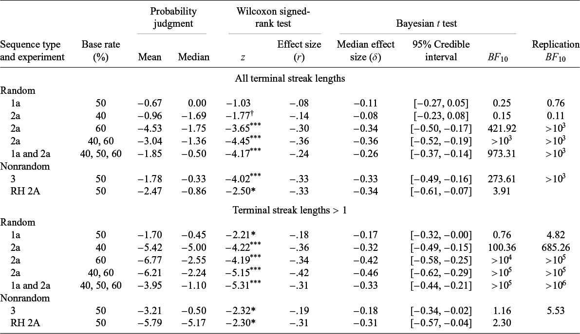

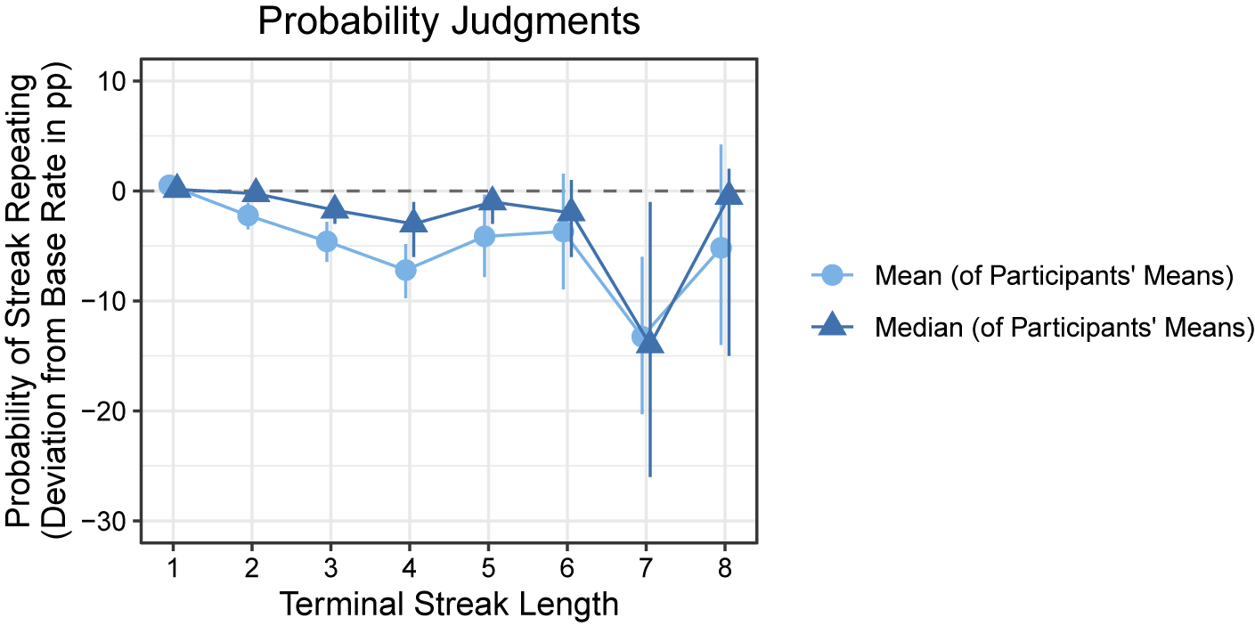
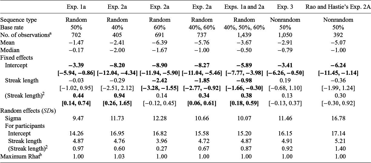
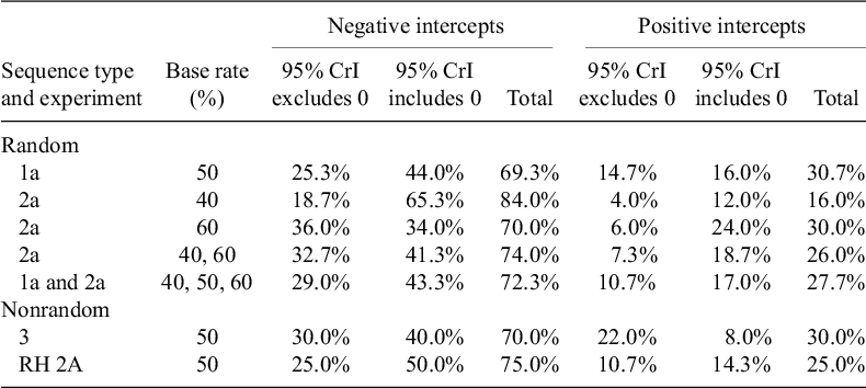


 Open access

