1 Introduction
Differential heating at the boundary of a stratified fluid arises in a variety of physical systems. The oceans and atmosphere are heated non-uniformly from above owing to the latitudinal variation of incoming solar energy. Fluid near the differentially heated surface moves laterally away from anomalously warm regions towards anomalously cold regions and a significant amount of work has considered whether this ‘horizontal convection’ can drive large-scale overturning circulations (e.g. Paparella & Young Reference Paparella and Young2002; Siggers, Kerswell & Balmforth Reference Siggers, Kerswell and Balmforth2004; Sheard, Hussam & Tsai Reference Sheard, Hussam and Tsai2016; Shishkina Reference Shishkina2017). The primary motivation for the present study is differential heating of planetary cores due to lateral heat flow anomalies in their overlying solid mantles. We conduct a systematic investigation of the interaction between thermal stratification and differential boundary heating, incorporating the key ingredients of rapid rotation and spherical shell geometry. Our main focus is to establish the extent to which boundary heat flow anomalies can penetrate and disrupt a pre-existing thermal stratification.
There is now a body of evidence indicating that the cores of Mercury (Christensen Reference Christensen2006), Earth (Davies et al.
Reference Davies, Pozzo, Gubbins and Alfè2015; Nimmo Reference Nimmo and Schubert2015), Mars (Stevenson Reference Stevenson2001) and Ganymede (Rückriemen, Breuer & Spohn Reference Rückriemen, Breuer and Spohn2015) are thermally stably stratified below the core–mantle boundary (CMB) owing to a subadiabatic CMB heat flow, with convection (and magnetic field generation) arising at greater depths. The existence of stratification is important because it influences the intensity and structure of the observable magnetic field (Christensen Reference Christensen2006; Stanley & Glatzmaier Reference Stanley and Glatzmaier2010) and reflects the core’s long-term evolution. The strength and thickness of these thermally stable regions is hard to assess due to a lack of direct observations. The stable layer in Earth’s core could be up to
 ${\sim}700~\text{km}$
thick (Gubbins et al.
Reference Gubbins, Alfè, Davies and Pozzo2015) with a Brunt–Väisälä frequency comparable to the rotation period. Thermal stratification in the Martian core is usually estimated to have begun around 4 Ga, corresponding to the epoch when the planet lost its global magnetic field (Stevenson Reference Stevenson2001), and so the thermally stable region could occupy a significant fraction of the present-day core. Thermal history models for Ganymede predict a stable layer hundreds of kilometres thick (Rückriemen et al.
Reference Rückriemen, Breuer and Spohn2015).
Terrestrial planetary cores are overlain by rocky mantle, which acts like a viscous fluid convecting on time scales of
 $10^{8}$
years. In contrast, liquid metal cores have very low viscosity and convect on time scales of
 $10^{3}$
years. This difference in convection time scales means that the core responds to the CMB as a rigid surface with a fixed heat flux imposed by the lower mantle, whilst the mantle is subjected to a uniform temperature lower boundary condition (Olson & Christensen Reference Olson and Christensen2002). Mantle convection simulations produce lateral temperature anomalies of thousands of Kelvin and lateral CMB heat flow variations greater than the mean CMB heat flow (e.g. Nakagawa & Tackley Reference Nakagawa and Tackley2008; Olson et al.
Reference Olson, Deguen, Rudolph and Zhong2015). These lateral variations will inevitably drive baroclinic flows in the underlying core through the thermal wind, but it is unclear the extent to which they will drive penetrative flow within a strongly stratified region.
The competition between stratification and boundary forcing has been explored in some numerical studies of convection in non-magnetic rotating spherical shells, which have shown that thermal boundary anomalies are capable of drastically altering the dynamics compared to uniform thermal boundary conditions (e.g. Zhang & Gubbins Reference Zhang and Gubbins1992, Reference Zhang and Gubbins1993; Gibbons & Gubbins Reference Gibbons and Gubbins2000; Gibbons, Gubbins & Zhang Reference Gibbons, Gubbins and Zhang2007). Zhang & Gubbins (Reference Zhang and Gubbins1992) solved for steady flows driven by lateral thermal variations at the outer boundary of a rotating spherical shell, having specified temperature rather than heat flux for numerical simplicity. They studied both unstratified and weakly stratified fluids subjected to a range of temperature anomaly patterns and magnitudes. For modest boundary anomaly strengths, patterns of temperature fluctuations and fluid flow lock to the boundary anomaly pattern through the thermal wind, and flows penetrate deep into the shell due to Coriolis effects. Stratification greatly reduces radial flow amplitudes, although toroidal flows are less affected, and confine flow towards the outer boundary. The authors speculated that these results would also be obtained in the geophysical case of fixed heat flux boundary anomalies. Gibbons & Gubbins (Reference Gibbons and Gubbins2000) were able to confirm this for steady flows in their subsequent investigation of weakly stratified fluids in rotating spherical shells. They applied different spatial distributions and magnitudes of large-scale boundary heat flow anomalies to fluids of varying stratification strengths. For equatorially symmetric patterns, rotational effects dominate the dynamics at weak or no stratification. As the stratification increases, rotational effects become less important, radial flow diminishes and flow is confined to a layer beneath the outer boundary. Smaller length scale heat-flux patterns drive less energetic flows that are not able to penetrate as deeply into the fluid. Solutions become increasingly smaller scale with increasing boundary anomaly magnitude, with correspondingly higher computational expense. Gibbons & Gubbins (Reference Gibbons and Gubbins2000) suggested that solutions would become unstable (time dependent) with sufficiently strong boundary anomalies, although computational limitations prevented the authors from identifying the parameters at which this occurs.
Several authors have considered the more realistic but more complex magnetohydrodynamic (MHD) case by studying numerical simulations of dynamos in partially stratified spherical shells, including Christensen (Reference Christensen2006), Christensen & Wicht (Reference Christensen and Wicht2008), Stanley & Mohammadi (Reference Stanley and Mohammadi2008), Aurnou & Aubert (Reference Aurnou and Aubert2011), Nakagawa (Reference Nakagawa2011), Nakagawa (Reference Nakagawa2015) and Olson, Landeau & Reynolds (Reference Olson, Landeau and Reynolds2017). Some numerical models have shown that the presence of a stable layer fundamentally changes dynamo action and can drastically alter the magnetic field at the planetary surface compared to equivalent models with no stable layer. For example, Christensen (Reference Christensen2006) showed that a strong magnetic field at the top of the dynamo generating region diffuses through a stable layer such that the small scale, rapidly varying components are filtered out.
Dynamo models with heterogeneous thermal boundary conditions have also been investigated by various authors, see the review by Amit et al. (Reference Amit, Choblet, Olson, Monteux, Deschamps, Langlais and Tobie2015) and references therein. As in the non-magnetic case, within MHD models heterogeneous boundary forcing has been shown to have a significant effect, for example by modifying the morphology of the magnetic field (e.g. Olson & Christensen Reference Olson and Christensen2002; Gubbins, Willis & Sreenivasan Reference Gubbins, Willis and Sreenivasan2007; Aurnou & Aubert Reference Aurnou and Aubert2011) such that its long-term fundamental symmetries follow the spatial symmetries of the imposed heat-flux pattern, or by locking the magnetic field to regions of anomalously high heat flow (Willis, Sreenivasan & Gubbins Reference Willis, Sreenivasan and Gubbins2007; Sreenivasan Reference Sreenivasan2009). In some circumstances, strong boundary-driven flows can also overwhelm the convection such that dynamo action is weakened or destroyed altogether (Olson & Christensen Reference Olson and Christensen2002; Takahashi et al. Reference Takahashi, Tsunakawa, Matsushima, Mochizuki and Honkura2008). Although ultimately the most physically relevant model, a thorough scaling analysis of the competition between stratification and boundary forcing within an MHD setting is beyond what is currently achievable. Some progress has been made by studying weakly stratified models with heterogeneous outer boundary conditions (e.g. Sreenivasan & Gubbins Reference Sreenivasan and Gubbins2008; Aurnou & Aubert Reference Aurnou and Aubert2011; Olson et al. Reference Olson, Landeau and Reynolds2017), although the extrapolation gap from the parameters used in these models to realistic values is large.
This work focusses on the simpler, non-magnetic problem which is yet not fully described. In particular, the previous studies described above have been limited to highly viscous, weakly stratified fluids in spherical shells with moderate rotation rates and subject to relatively weak boundary anomalies: it is not clear how these results bear on the rapidly rotating, strongly stratified case relevant to planetary cores that are additionally subject to significant lateral variations in heat flux at their outer boundary. One severe computational limitation that has hampered progress arises because rotating flows adopt small azimuthal length scales even at the onset of convection (Chandrasekhar Reference Chandrasekhar1961), while increasing the amplitude of the driving force generates a broad spectrum of flow structures that become increasingly difficult to resolve. In this study, we minimise this problem by considering a subset of steady-state solutions obtained from solving the full time-dependent equations, and also by assuming that the entire fluid domain is stably stratified without any internal heat sources that drive internal convection. This is equivalent to assuming that any underlying convection does not significantly penetrate or mix an overlying stable region, which is true in the case of strong stratification (Takehiro & Lister Reference Takehiro and Lister2001; Buffett & Seagle Reference Buffett and Seagle2010; Gubbins & Davies Reference Gubbins and Davies2013). These assumptions allow us to isolate the interaction between outer boundary forcing and pre-existing stratification, without the additional complication of destabilisation of stratified fluid from below by internal convection, and to study the dynamics using a much wider range of parameters than has been possible previously.
The fluid dynamical problem we consider depends upon three dimensionless numbers (detailed definitions are given in 2.1): a thermal stratification parameter,
 $S$
, defined as the relative size of boundary temperature gradients to imposed vertical temperature gradients, a buoyancy parameter,
 $B$
, measuring the strength of the applied boundary heat-flux anomalies, and the Ekman number,
 $E$
, the ratio of viscous and Coriolis forces. Our study spans the ranges
 $10^{-2}\leqslant B\leqslant 10^{6}$
,
 $10^{-3}\leqslant S\leqslant 10^{4}$
and
 $10^{-6}\leqslant E\leqslant 10^{-4}$
. We focus primarily on the case where the aspect ratio, the ratio of inner to outer boundary radii, corresponds to that of Earth’s liquid core,
 $r_{i}/r_{o}=\unicode[STIX]{x1D702}=0.35$
. Additional simulations are performed at
 $\unicode[STIX]{x1D702}=0.01$
, which is almost a full sphere and approximates the core geometry of Mars and Ganymede.
For each choice of
 $(E,S,B)$
a heat flow pattern must be chosen. Previous studies clearly show that the influence of thermal boundary anomalies on the structure and dynamics of rotating fluids becomes more pronounced as the length scale of the imposed pattern is increased (Zhang & Gubbins Reference Zhang and Gubbins1992, Reference Zhang and Gubbins1993; Davies, Gubbins & Jimack Reference Davies, Gubbins and Jimack2009). We choose to apply a
 $Y_{2}^{2}$
spherical harmonic boundary heat flow pattern since this the largest component of shear-wave variation (a likely proxy for CMB heat flow) in Earth’s lower mantle (Dziewonski, Lekic & Romanowicz Reference Dziewonski, Lekic and Romanowicz2010); it is also a common boundary condition of previous studies, which makes comparison straightforward (e.g. Zhang & Gubbins Reference Zhang and Gubbins1992, Reference Zhang and Gubbins1993; Davies et al.
Reference Davies, Gubbins and Jimack2009; Sreenivasan Reference Sreenivasan2009; Sahoo & Sreenivasan Reference Sahoo and Sreenivasan2017).
We have conducted a suite of 99 numerical simulations finding predominantly steady solutions, which partition into two distinct regimes. Within each regime we formulate theoretical scaling laws that provide excellent fits to our dataset and permit extrapolation to the parameter regimes appropriate to planetary interiors. The remainder of the paper is structured as follows: the mathematical formulation is given in § 2, results of the numerical simulations are presented in § 3, scaling analyses and their application to Earth and Ganymede’s outer cores follow in §§ 4 and 5 and a summary of results is found in § 6.
2 Method
We consider an incompressible Boussinesq fluid in an impenetrable spherical shell, of outer radius
 $r_{o}$
and inner radius
 $r_{i}$
, rotating about the axial
 $\hat{\boldsymbol{z}}$
direction with constant angular velocity
 $\unicode[STIX]{x1D6FA}$
. The whole shell is thermally stratified and compositional effects are neglected, as in Gibbons & Gubbins (Reference Gibbons and Gubbins2000), in order to isolate the effects of thermal boundary anomalies on a thermally stratified fluid. Again following Gibbons & Gubbins (Reference Gibbons and Gubbins2000), we also neglect the magnetic field so as to reach more realistic
 $E$
,
 $B$
and
 $S$
values; the effects of free convection and the resulting magnetic field evolution will be investigated in a future study. In the following work,
 $r$
,
 $\unicode[STIX]{x1D703}$
and
 $\unicode[STIX]{x1D719}$
denote spherical polar coordinates,
 $\boldsymbol{r}$
is the position vector and
 $t$
is time.
2.1 Governing equations and non-dimensionalisation
Following the formulation of Zhang & Gubbins (Reference Zhang and Gubbins1992) and Gibbons & Gubbins (Reference Gibbons and Gubbins2000), the temperature is split into a steady radial part,
 $T_{0}$
, and a time-varying part,
 $T_{1}$
, such that
 $$\begin{eqnarray}T(r,\unicode[STIX]{x1D703},\unicode[STIX]{x1D719},t)=T_{0}(r)+T_{1}(r,\unicode[STIX]{x1D703},\unicode[STIX]{x1D719},t).\end{eqnarray}$$
The steady radial temperature profile satisfies
 $$\begin{eqnarray}\unicode[STIX]{x1D705}\unicode[STIX]{x1D6FB}^{2}T_{0}=F,\end{eqnarray}$$
where
 $\unicode[STIX]{x1D705}$
is the thermal diffusivity and
 $F\geqslant 0$
is a heat sink that is chosen to impose a background thermal gradient that, if strong, suppresses radial motion. Integrating with respect to
 $r$
in spherical coordinates gives
 $$\begin{eqnarray}r^{2}\frac{\text{d}T_{0}}{\text{d}r}=\unicode[STIX]{x1D6FD}r^{3}+A,\end{eqnarray}$$
where
 $\unicode[STIX]{x1D6FD}=F/3\unicode[STIX]{x1D705}$
and
 $A$
is a constant of integration. Setting the outer boundary condition such that
 $$\begin{eqnarray}\left.\frac{\text{d}T_{0}}{\text{d}r}\right|_{r=r_{o}}=\unicode[STIX]{x1D6FD}r_{o}\end{eqnarray}$$
results in
 $A=0$
and so within the spherical shell
 $\text{d}T_{0}/\text{d}r=\unicode[STIX]{x1D6FD}r$
.
We define the outer boundary condition of the temperature gradient as
 $$\begin{eqnarray}\left.\frac{\unicode[STIX]{x2202}T_{1}}{\unicode[STIX]{x2202}r}\right|_{r=r_{o}}={\mathcal{H}}Y_{2}^{2}(\unicode[STIX]{x1D703},\unicode[STIX]{x1D719}),\end{eqnarray}$$
in which the spatial pattern of the anomaly is given by the spherical harmonic
 $Y_{2}^{2}(\unicode[STIX]{x1D703},\unicode[STIX]{x1D719})$
, and the magnitude of the anomaly is given by
 ${\mathcal{H}}$
. Rewriting the general temperature equation
 $$\begin{eqnarray}\frac{\unicode[STIX]{x2202}T}{\unicode[STIX]{x2202}t}+(\boldsymbol{u}\boldsymbol{\cdot }\unicode[STIX]{x1D735})T=\unicode[STIX]{x1D705}\unicode[STIX]{x1D6FB}^{2}T-F,\end{eqnarray}$$
 $$\begin{eqnarray}\frac{\unicode[STIX]{x2202}T_{1}}{\unicode[STIX]{x2202}t}+(\boldsymbol{u}\boldsymbol{\cdot }\unicode[STIX]{x1D735})T_{1}+u_{r}\unicode[STIX]{x1D6FD}r=\unicode[STIX]{x1D705}\unicode[STIX]{x1D6FB}^{2}T_{1}\end{eqnarray}$$
as the temperature equation.
The equations for conservation of momentum in a rotating frame of reference and for conservation of mass are
 $$\begin{eqnarray}\frac{\unicode[STIX]{x2202}\boldsymbol{u}}{\unicode[STIX]{x2202}t}+(\boldsymbol{u}\boldsymbol{\cdot }\unicode[STIX]{x1D735})\boldsymbol{u}+2\unicode[STIX]{x1D6FA}(\hat{\boldsymbol{z}}\times \boldsymbol{u})=-\unicode[STIX]{x1D735}\left(\frac{P^{\prime }}{\unicode[STIX]{x1D70C}_{0}}\right)+\frac{\unicode[STIX]{x1D70C}^{\prime }\boldsymbol{g}}{\unicode[STIX]{x1D70C}_{0}}+\unicode[STIX]{x1D708}\unicode[STIX]{x1D6FB}^{2}\boldsymbol{u}\end{eqnarray}$$
and
 $$\begin{eqnarray}\unicode[STIX]{x1D735}\boldsymbol{\cdot }\boldsymbol{u}=0,\end{eqnarray}$$
where
 $\boldsymbol{u}$
is velocity,
 $P^{\prime }$
is the pressure perturbation,
 $\unicode[STIX]{x1D70C}_{0}$
is a reference density,
 $\unicode[STIX]{x1D70C}^{\prime }$
is the deviation from the reference density,
 $\boldsymbol{g}$
is gravity and
 $\unicode[STIX]{x1D708}$
is the kinematic viscosity. Expressing
 $\unicode[STIX]{x1D70C}^{\prime }$
as
 $$\begin{eqnarray}\unicode[STIX]{x1D70C}^{\prime }=-\unicode[STIX]{x1D70C}_{0}\unicode[STIX]{x1D6FC}_{T}T_{1},\end{eqnarray}$$
where
 $\unicode[STIX]{x1D6FC}_{T}$
is the coefficient of thermal expansivity, gives an alternative form of the momentum equation
 $$\begin{eqnarray}\frac{\unicode[STIX]{x2202}\boldsymbol{u}}{\unicode[STIX]{x2202}t}+(\boldsymbol{u}\boldsymbol{\cdot }\unicode[STIX]{x1D735})\boldsymbol{u}+2\unicode[STIX]{x1D6FA}(\hat{\boldsymbol{z}}\times \boldsymbol{u})=-\unicode[STIX]{x1D735}\hat{P}+\unicode[STIX]{x1D6FC}_{T}\unicode[STIX]{x1D6FE}T_{1}\boldsymbol{r}+\unicode[STIX]{x1D708}\unicode[STIX]{x1D6FB}^{2}\boldsymbol{u},\end{eqnarray}$$
where
 $\hat{P}$
is the reduced pressure (
 $=P^{\prime }/\unicode[STIX]{x1D70C}_{0}$
) and
 $\unicode[STIX]{x1D6FE}$
is a constant (
 $\boldsymbol{g}=-\unicode[STIX]{x1D6FE}\boldsymbol{r}$
).
Scaling radius by a characteristic length scale
 $d$
(
 $=r_{o}-r_{i}$
), time by the thermal diffusion time
 $d^{2}/\unicode[STIX]{x1D705}$
, velocity by
 $\unicode[STIX]{x1D705}/d$
and temperature by
 ${\mathcal{H}}d$
(from (2.5)) gives the radial temperature profile and the temperature and momentum equations in their dimensionless forms
 $$\begin{eqnarray}\displaystyle & \displaystyle \frac{\text{d}T_{0}^{\ast }}{\text{d}r^{\ast }}=Sr^{\ast }, & \displaystyle\end{eqnarray}$$
 $$\begin{eqnarray}\displaystyle & \displaystyle \frac{\unicode[STIX]{x2202}T_{1}^{\ast }}{\unicode[STIX]{x2202}t^{\ast }}+(\boldsymbol{u}^{\ast }\boldsymbol{\cdot }\unicode[STIX]{x1D735})T_{1}^{\ast }+Su_{r}^{\ast }r^{\ast }=\unicode[STIX]{x1D6FB}^{2}T_{1}^{\ast } & \displaystyle\end{eqnarray}$$
and
 $$\begin{eqnarray}\frac{E}{Pr}\left[\frac{\unicode[STIX]{x2202}\boldsymbol{u}^{\ast }}{\unicode[STIX]{x2202}t^{\ast }}+(\boldsymbol{u}^{\ast }\boldsymbol{\cdot }\unicode[STIX]{x1D735})\boldsymbol{u}^{\ast }\right]+(\hat{\boldsymbol{z}}^{\ast }\times \boldsymbol{u}^{\ast })=-\unicode[STIX]{x1D735}\hat{P}+BT_{1}^{\ast }\boldsymbol{r}^{\ast }+E\unicode[STIX]{x1D6FB}^{2}\boldsymbol{u}^{\ast },\end{eqnarray}$$
where
 $\boldsymbol{r}^{\ast }$
is the dimensionless radial vector,
 $S$
is the stratification parameter,
 $E$
is the Ekman number,
 $Pr$
is the Prandtl number and
 $B$
is the buoyancy parameter. These dimensionless numbers are defined as
 $$\begin{eqnarray}S=\frac{\unicode[STIX]{x1D6FD}d}{{\mathcal{H}}},\quad E=\frac{\unicode[STIX]{x1D708}}{2\unicode[STIX]{x1D6FA}d^{2}},\quad Pr=\frac{\unicode[STIX]{x1D708}}{\unicode[STIX]{x1D705}},\quad B=\frac{\unicode[STIX]{x1D6FC}_{T}\unicode[STIX]{x1D6FE}{\mathcal{H}}d^{3}}{2\unicode[STIX]{x1D6FA}\unicode[STIX]{x1D705}},\end{eqnarray}$$
and
 $B$
is related to
 $E$
and a Rayleigh number,
 $Ra_{{\mathcal{H}}}$
, where
 $$\begin{eqnarray}\frac{B}{E}=Ra_{{\mathcal{H}}}=\frac{\unicode[STIX]{x1D6FC}_{T}\unicode[STIX]{x1D6FE}{\mathcal{H}}d^{5}}{\unicode[STIX]{x1D708}\unicode[STIX]{x1D705}}.\end{eqnarray}$$
In this work, all calculations are performed at
 $Pr=1$
for numerical convenience and the majority with a shell aspect ratio
 $\unicode[STIX]{x1D702}=0.35$
; a summary of model parameters is given in tables 3–6 in appendix A. We investigate the effects of varying the shell aspect ratio using models with
 $\unicode[STIX]{x1D702}=0.01$
in § 4.3. The governing equations are solved for
 $\boldsymbol{u}$
and
 $T_{1}$
with no-slip boundary conditions on both inner and outer boundaries, a fixed temperature of zero imposed on the inner boundary and a fixed heat flux imposed on the outer boundary, as previously discussed. A detailed description of the pseudo-spectral code may be found in Willis et al. (Reference Willis, Sreenivasan and Gubbins2007) and Davies, Gubbins & Jimack (Reference Davies, Gubbins and Jimack2011), and in the most recent dynamo benchmark paper (Matsui et al.
Reference Matsui, Heien, Aubert, Aurnou, Avery, Brown, Buffett, Busse, Christensen, Davies, Featherstone, Gastine, Glatzmaier, Gubbins, Guermond, Hayashi, Hollerbach, Hwang, Jackson, Jones, Jiang, Kellogg, Kuang, Landeau, Marti, Olson, Ribeiro, Sasaki, Schaeffer, Simitev, Sheyko, Silva, Stanley, Takahashi, Takehiro, Wicht and Willis2016). Although (2.1)–(2.5) give the clearest mathematical description of our method, in fact the code solves the following equation
 $$\begin{eqnarray}\frac{\unicode[STIX]{x2202}T^{\ast }}{\unicode[STIX]{x2202}t^{\ast }}+(\boldsymbol{u}^{\ast }\boldsymbol{\cdot }\unicode[STIX]{x1D735})T^{\ast }=\unicode[STIX]{x1D6FB}^{2}T^{\ast }-3S,\end{eqnarray}$$
which is equivalent to (2.13). To benchmark our code for this particular problem, we reproduced the flow magnitudes and spatial patterns reported in Gibbons & Gubbins (Reference Gibbons and Gubbins2000), using a shell aspect ratio
 $\unicode[STIX]{x1D702}=0.4$
and their parameters of
 $E=10^{-3}$
,
 $Pr=1$
,
 $B=1$
and
 $S=0$
and
 $S=100$
.
Given that we focus upon steady-state solutions to the time-dependent equations, for numerical expediency where possible we used the final steady-state solution of a model nearby in parameter space as the initial condition. Models were run long past the initial transient period and until the volume-averaged kinetic energy converged to a steady value. Several numerical models were unstable and no steady-state solutions were obtained at those parameters. In such cases, we cannot rule out the existence of a steady-state model using different initial conditions.
For each of our models, spatial convergence was verified by assessing the kinetic energy power spectrum as a function of spherical harmonic degree (
 $l$
) and order (
 $m$
). For all models, the maximum power was found at long wavelengths (the lowest
 $l$
), which generally exceeded the power in the shortest wavelengths (high
 $l$
) by a large amount: at least two, although usually four or five, orders of magnitude.
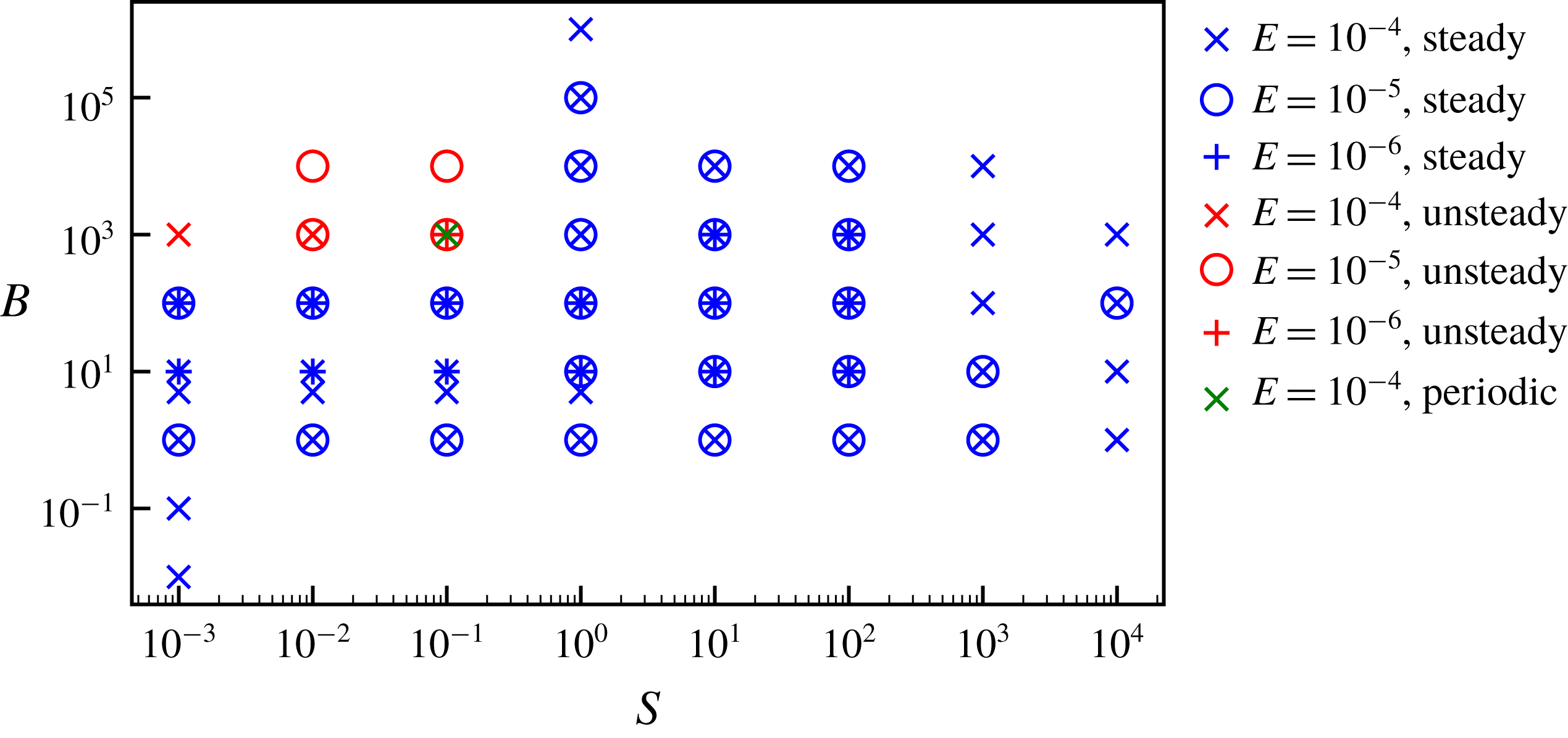
Figure 1 is a stability diagram showing regions of parameter space resulting in steady and unsteady solutions. The figure shows the transition between high
 $B$
and low
 $S$
models, which are unsteady, and higher
 $S$
models, which produce a steady state. One periodic model was obtained at the boundary between the steady and unsteady regions of parameter space. In the remainder of this work, we focus our attention upon the steady-state regime; time-dependent models are the subject of a future paper.
Stability diagram in (
 $S$
,
 $B$
) parameter space showing all models summarised in tables 3–5. The symbol type represents the Ekman number (crosses denote
 $E=10^{-4}$
, circles denote
 $E=10^{-5}$
and plus signs denote
 $E=10^{-6}$
); the symbol colour represents the stability of the solution obtained (blue denotes a steady-state solution, red denotes a time-dependent solution and green denotes a periodic solution).

3 Results
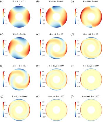
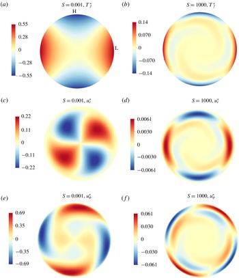
Figure 2 shows the temperature perturbations in the equatorial plane, denoted
 $T_{f}^{\ast }$
, for models at
 $E=10^{-4}$
and a range of
 $B$
and
 $S$
values. Note that in the remainder of this text, we use
 $T_{f}^{\ast }$
(the fluctuating part of the temperature) as a proxy for
 $T_{1}^{\ast }$
defined in (2.1). To calculate the quantity
 $T_{f}^{\ast }$
, the
 $Y_{0}^{0}$
spherical harmonic component of the total temperature
 $T^{\ast }$
has been removed, which includes all of
 $T_{0}^{\ast }$
and also the mean of
 $T_{1}^{\ast }$
. Therefore,
 $T_{f}^{\ast }$
and
 $T_{1}^{\ast }$
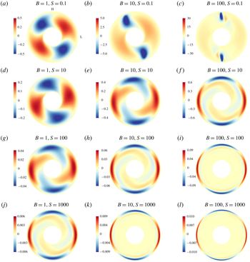
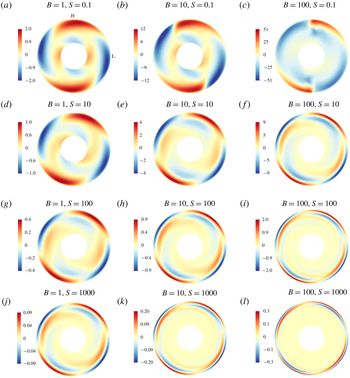
differ in that the former is zero mean and the latter is not. Figures 3 and 4 show the radial and azimuthal velocity components,
 $u_{r}^{\ast }$
and
 $u_{\unicode[STIX]{x1D719}}^{\ast }$
, for the same models. At low
 $B$
and
 $S$
, the temperature fluctuations are large scale with a
 $Y_{2}^{2}$
spatial pattern locked to the applied heat-flux pattern on the outer boundary and penetrating through the whole shell depth. The two lobes of negative temperature (blue) correspond to regions of high outward heat flux and the two lobes of positive temperature (red) correspond to regions of low outward heat flux. Zeroes of
 $T_{f}^{\ast }$
(at
 $\unicode[STIX]{x1D719}\approx \unicode[STIX]{x03C0}/4,3\unicode[STIX]{x03C0}/4,5\unicode[STIX]{x03C0}/4,7\unicode[STIX]{x03C0}/4$
) correspond to locations of the outer boundary heat flux changing sign. The radial velocity is dominated by large-scale convection cells that occupy the whole shell, with two upwellings and two downwellings present, and the peak velocity amplitudes occur at approximately half the shell radius. The lateral locations of these maxima and minima approximately correspond to locations of
 $T_{f}^{\ast }=0$
. In azimuthal velocity, locations of diverging (converging) lobes of opposite sign correspond to locations of upwellings (downwellings) of radial flow and
 $T_{f}^{\ast }=0$
.
As the stratification parameter (
 $S$
) increases, temperature perturbations and flow magnitudes decrease and the dynamics becomes concentrated towards the outer boundary rather than occupying the entire shell thickness. Radial flow cells begin to elongate near the inner boundary, and high velocity magnitudes are concentrated near the outer boundary rather than the inner boundary. In
 $u_{\unicode[STIX]{x1D719}}^{\ast }$
, inner and outer cells of the same polarity begin to join together through tails trailing from the outermost cells, with the inner cells decreasing in amplitude. Radial flow is strongly suppressed with increasing
 $S$
, which is expected because stratification does not permit large radial velocities. Azimuthal flow is only weakly suppressed with increasing stratification as horizontal flows are permitted within a stably stratified layer. At high
 $S$
, all flow becomes confined to a thin shear layer of thickness
 $\unicode[STIX]{x1D6FF}^{\ast }$
beneath the outer boundary (hereafter referred to as the ‘penetration depth’ into the fluid).
As
 $B$
increases, temperature perturbations decrease and flow magnitudes increase. This is a consequence of the fixed heat-flux outer boundary condition; increasing the buoyancy produces stronger flows that better homogenise the temperature, resulting in velocity increasing with
 $B$
while temperature perturbations decrease (e.g. Otero et al.
Reference Otero, Wittenberg, Worthing and Doering2002; Mound & Davies Reference Mound and Davies2017). Flows are phase shifted so that upwellings (and diverging
 $u_{\unicode[STIX]{x1D719}}^{\ast }$
) and downwellings (and converging
 $u_{\unicode[STIX]{x1D719}}^{\ast }$
) are now locked to the boundary pattern itself rather to locations of heat flux changing sign. Upwellings (downwellings) are beneath high (low) boundary heat flow regions. At low
 $S$
and increasing
 $B$
(e.g. figures 2–4(a–c)), temperature and flow patterns are strikingly different from models at other parameters. Downwellings become increasingly faster and much narrower in azimuth with increasing
 $B$
, although still occupying the whole shell radius, whilst the upwellings remain broad and low amplitude. This pattern of slow, broad upwellings and fast, narrow downwellings in the presence of lateral boundary anomalies was also obtained in e.g. Willis et al. (Reference Willis, Sreenivasan and Gubbins2007), Sreenivasan & Gubbins (Reference Sreenivasan and Gubbins2011). At higher
 $S$
, upwellings and downwellings are of similar lateral extent and the dynamics is confined to a thin shear layer whose thickness decreases with increasing
 $S$
and
 $B$
.
Equatorial plots of
 $T_{f}^{\ast }$
for models at
 $E=10^{-4}$
and varying
 $S$
(increasing from top to bottom) and
 $B$
(increasing from left to right). Red indicates positive values and blue indicates negative values. Note the different colour scales. Locations of high (H) and low (L) outward heat flux are shown on (a).

Equatorial plots of
 $u_{r}^{\ast }$
for models at
 $E=10^{-4}$
and varying
 $S$
(increasing from top to bottom) and
 $B$
(increasing from left to right). Red indicates positive values and blue indicates negative values. Note the different colour scales. Locations of high (H) and low (L) outward heat flux are shown on (a).

Equatorial plots of
 $u_{\unicode[STIX]{x1D719}}^{\ast }$
for models at
 $E=10^{-4}$
and varying
 $S$
(increasing from top to bottom) and
 $B$
(increasing from left to right). Red indicates positive values and blue indicates negative values. Note the different colour scales. Locations of high (H) and low (L) outward heat flux are shown on (a).

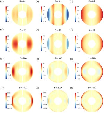
Figure 5 shows
 $u_{r}^{\ast }$
(a,d,g,j) and
 $u_{\unicode[STIX]{x1D719}}^{\ast }$
(b,e,h,k) and
 $T_{f}^{\ast }$
(c,f,i,l) in a meridional plane for models run at
 $E=10^{-4}$
and
 $B=1$
for a range of stratification parameters (
 $S$
). At low
 $S$
, the dynamics is dominated by large-scale features that are aligned with the rotation axis. There is little variation parallel to the
 $z$
-axis, as expected in a rapidly rotating system from the Taylor–Proudman theorem. As stratification increases, the dynamics is confined to the shear layer at the top of the shell, as seen in figures 2–4, which means that significant
 $z$
variations now occur in the models of the order of the penetration depth,
 $\unicode[STIX]{x1D6FF}^{\ast }$
.
Meridional plots of
 $u_{r}^{\ast }$
(a,d,g,j),
 $u_{\unicode[STIX]{x1D703}}^{\ast }$
(b,e,h,k) and
 $T_{f}^{\ast }$
(c,f,i,l) for models at
 $E=10^{-4}$
,
 $B=1$
and varying
 $S$
(increasing from top to bottom). Red indicates positive values and blue indicates negative values.

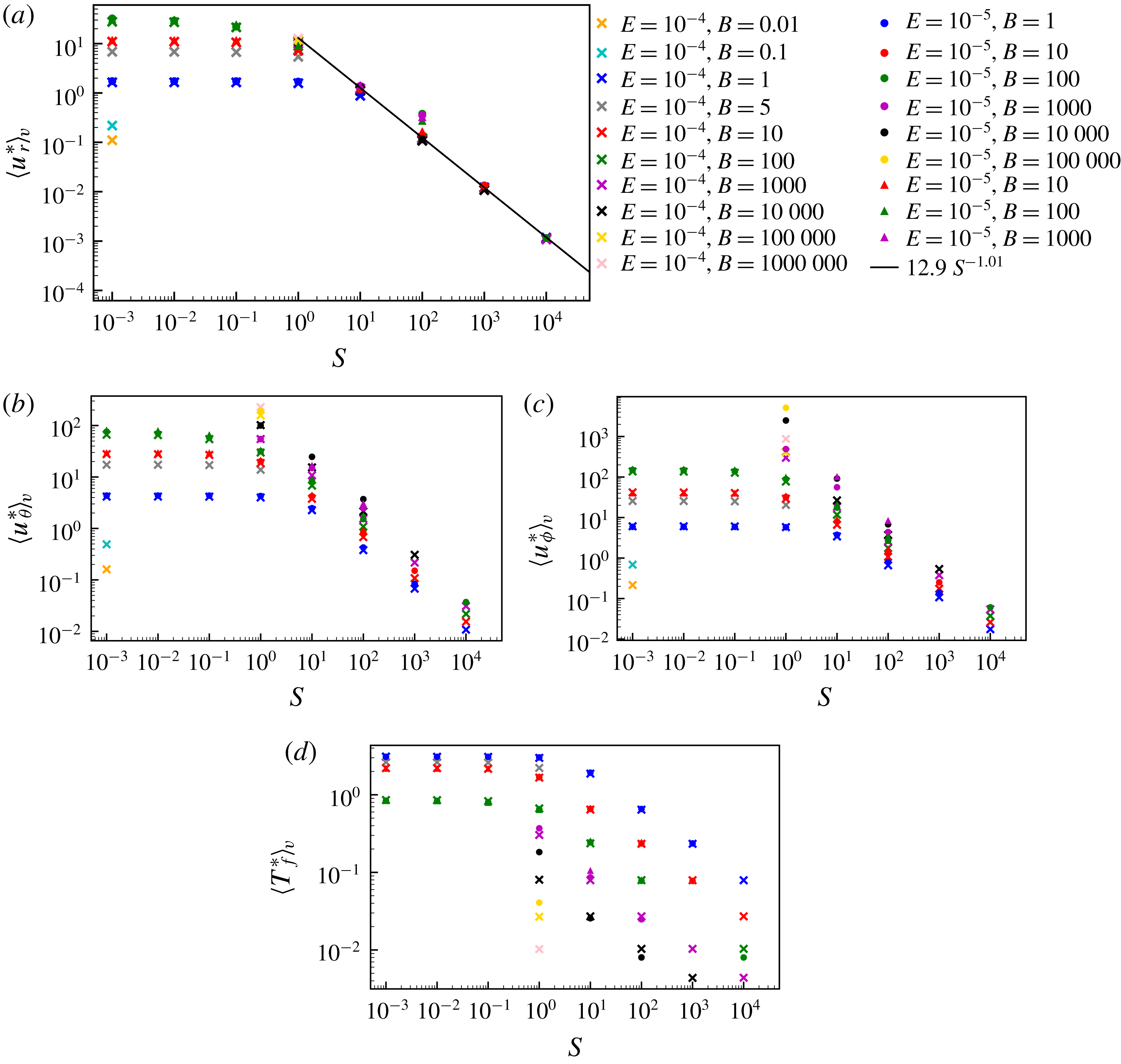
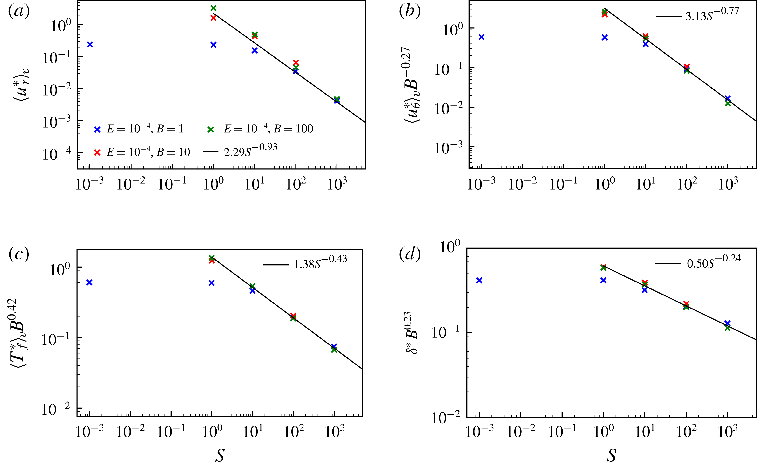
Volume-averaged values of the absolute (a) radial velocity,
 $\langle u_{r}^{\ast }\rangle _{v}$
, (b) meridional velocity,
 $\langle u_{\unicode[STIX]{x1D703}}^{\ast }\rangle _{v}$
, (c) azimuthal velocity,
 $\langle u_{\unicode[STIX]{x1D719}}^{\ast }\rangle _{v}$
and (d) temperature perturbations,
 $\langle T_{f}^{\ast }\rangle _{v}$
, as a function of the stratification parameter,
 $S$
, for all steady models. Symbol shapes represent the Ekman number,
 $E$
, and colours represent the buoyancy parameter,
 $B$
. The black line in panel (a) is the power law best fit for all models at
 $S>1$
.

Figure 6 shows
 $\langle u_{r}^{\ast }\rangle _{v}$
,
 $\langle u_{\unicode[STIX]{x1D719}}^{\ast }\rangle _{v}$
,
 $\langle v_{\unicode[STIX]{x1D703}}^{\ast }\rangle _{v}$
and
 $\langle T_{f}^{\ast }\rangle _{v}$
, where the angular brackets denote the magnitude averaged over the shell volume
 $V$
such that, for example,
 $\langle u_{r}^{\ast }\rangle _{v}=\int |u_{r}^{\ast }|\,\text{d}V$
, and likewise for vector quantities. We define a similar operator for the integral over a surface
 $S$
of radius
 $r$
such that
 $\langle u_{r}^{\ast }\rangle _{s}=(1/S)\int |u_{r}^{\ast }|\,\text{d}S$
. We adopt an average over the entire domain, rather than only the shear layer volume, because it is difficult to estimate the exact location of the shear layer edge. We assume that the quantities of interest are dominated by their values within the shear layer, with negligible contribution from elsewhere in the domain, such that our volume-averaged quantities are representative of the shear layer volume average. Furthermore, we use the average of the modulus because integration over solid angle would otherwise result in large-scale cancellation due to the spherical symmetry of the problem. The volume-averaged quantities show a clear transition from the low stratification (
 $S$
) regime, in which the dynamics appears to be related to
 $B$
and
 $E$
only, and the high
 $S$
regime, in which stratification dominates the dynamics and the quantities obey power law relationships in both
 $S$
and
 $B$
.
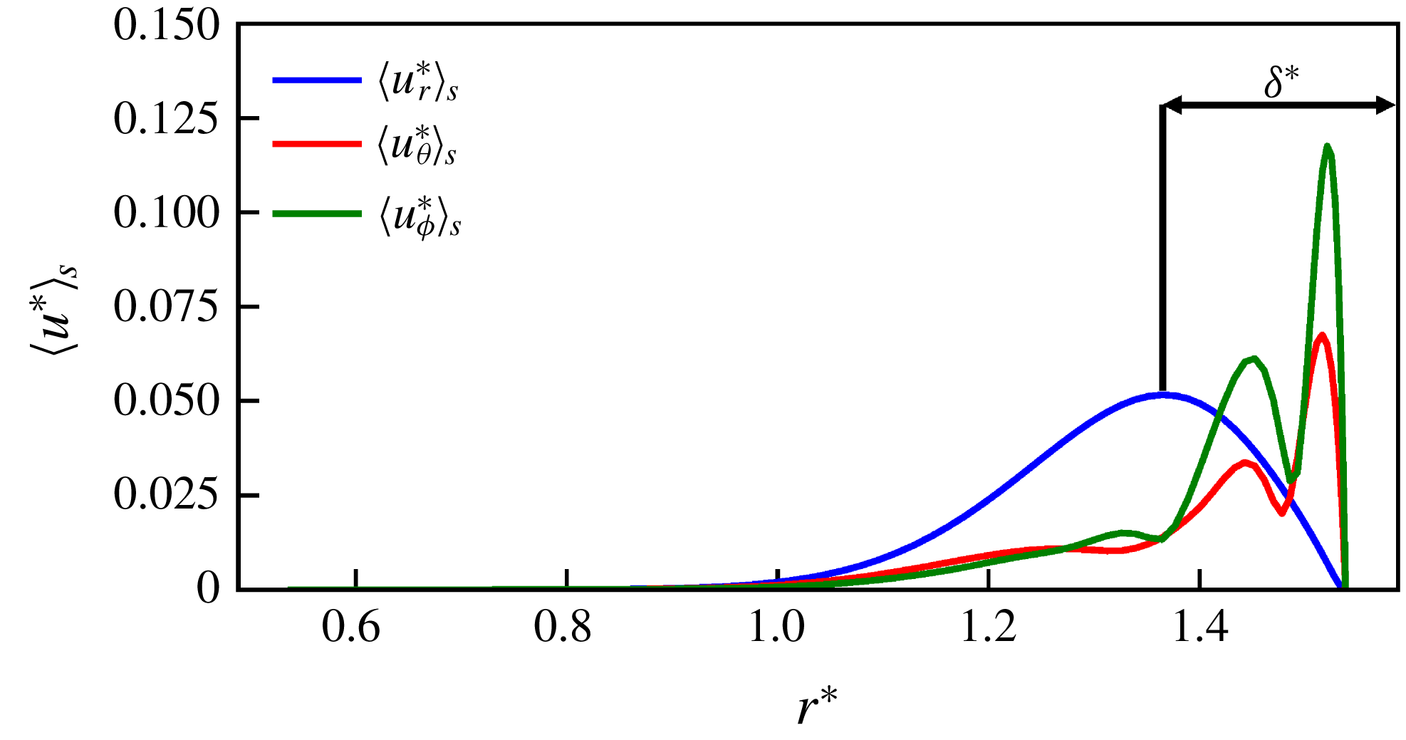
We use the location of the peak in
 $\langle u_{r}^{\ast }\rangle _{s}$
as a function of radius to estimate the penetration depth,
 $\unicode[STIX]{x1D6FF}^{\ast }$
, for each model. We define the radius of maximum
 $\langle u_{r}^{\ast }\rangle _{s}$
as
 $r_{max}$
and calculate the penetration depth as follows
 $$\begin{eqnarray}\unicode[STIX]{x1D6FF}^{\ast }=r_{o}-r_{max}.\end{eqnarray}$$
Radial velocity is used to estimate the penetration depth because it has only a single peak that is located centrally within the shear layer, whereas the horizontal components typically have several peaks, with the highest value close to the outer boundary in our
 $S>1$
models (see the equatorial sections in figures 3 and 4, and figure 7 for a representative example of radial velocity profiles). Note that the
 $\langle \rangle _{s}$
operation averages any longitudinal dependence of
 $u_{r}^{\ast }$
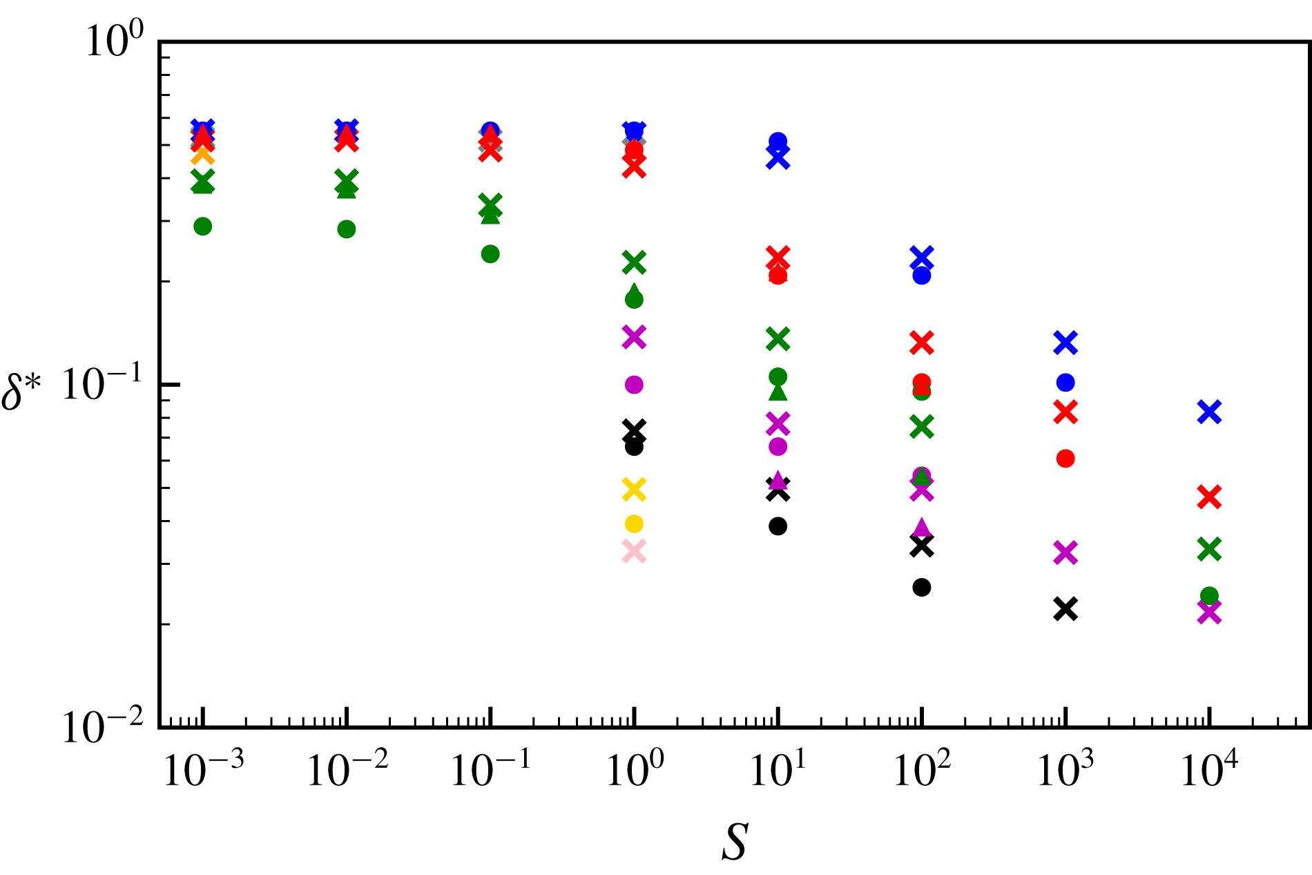
, as seen in figure 5 for example. Figure 8 shows that
 $\unicode[STIX]{x1D6FF}^{\ast }$
has different behaviour in the two stratification (
 $S$
) regimes, with
 $\unicode[STIX]{x1D6FF}^{\ast }$
of the order of the shell thickness at low
 $S$
and obeying power law relationships in
 $S$
and
 $B$
.
Components of velocity as a function of radius for a model run at
 $E=10^{-4}$
,
 $B=100$
and
 $S=1000$
. The line colour denotes the flow component (blue for radial, red for meridional and green for azimuthal). The black arrow represents the width used as an estimate for the penetration depth,
 $\unicode[STIX]{x1D6FF}^{\ast }$
, in this model (calculated according to (3.1)).

Estimates of the penetration depth
 $\unicode[STIX]{x1D6FF}^{\ast }$
, as a function of the stratification parameter,
 $S$
, for all steady models. Symbol shapes represent the Ekman number,
 $E$
, and colours represent the buoyancy parameter,
 $B$
. The key is given in figure 6(a).

4 Scaling analysis
In this section, our aim is to recover power laws of the form
 $$\begin{eqnarray}f=S^{a}B^{b}\end{eqnarray}$$
from the governing equations to express the velocity components, temperature fluctuations and penetration depth (denoted
 $f$
above) as functions of the control parameters
 $S$
and
 $B$
(and, equivalently,
 $S$
,
 $Ra_{{\mathcal{H}}}$
and
 $E$
), where coefficients
 $a$
and
 $b$
are to be determined. We then verify these predicted scalings for our models using the volume-averaged quantities introduced above, and finally we extrapolate the power laws to planetary core conditions.
4.1 High stratification regime
At high stratification parameter,
 $S$
, flow is confined to a shear layer of thickness
 $\unicode[STIX]{x1D6FF}^{\ast }$
at the top of the shell and this penetration depth decreases with increasing stratification. Within the layer, flow tends to be in long, thin lobes with relatively little lateral variation, which suggests that the radial gradients of velocity (
 $\unicode[STIX]{x2202}/\unicode[STIX]{x2202}r^{\ast }$
) are larger than the horizontal (
 $\unicode[STIX]{x2202}/\unicode[STIX]{x2202}\unicode[STIX]{x1D703}^{\ast }$
and
 $\unicode[STIX]{x2202}/\unicode[STIX]{x2202}\unicode[STIX]{x1D719}^{\ast }$
) gradients. Our dimensionless horizontal lengths are
 $O(1)$
and the relevant radial length scale is
 $O(\unicode[STIX]{x1D6FF}^{\ast })$
so that the continuity equation (2.9) gives a relationship between the velocity components
 $$\begin{eqnarray}u_{r}^{\ast }\sim \unicode[STIX]{x1D6FF}^{\ast }u_{\unicode[STIX]{x1D703}}^{\ast }\sim \unicode[STIX]{x1D6FF}^{\ast }u_{\unicode[STIX]{x1D719}}^{\ast },\end{eqnarray}$$
assuming that
 $\unicode[STIX]{x2202}/\unicode[STIX]{x2202}\unicode[STIX]{x1D703}^{\ast }\sim \unicode[STIX]{x2202}/\unicode[STIX]{x2202}\unicode[STIX]{x1D719}^{\ast }$
. Adherence of our high
 $S$
models to this scaling was verified using the estimates of
 $\unicode[STIX]{x1D6FF}^{\ast }$
shown in figure 8 and volume-averaged velocities
 $\langle u_{r}^{\ast }\rangle _{v}$
,
 $\langle u_{\unicode[STIX]{x1D703}}^{\ast }\rangle _{v}$
and
 $\langle u_{\unicode[STIX]{x1D719}}^{\ast }\rangle _{v}$
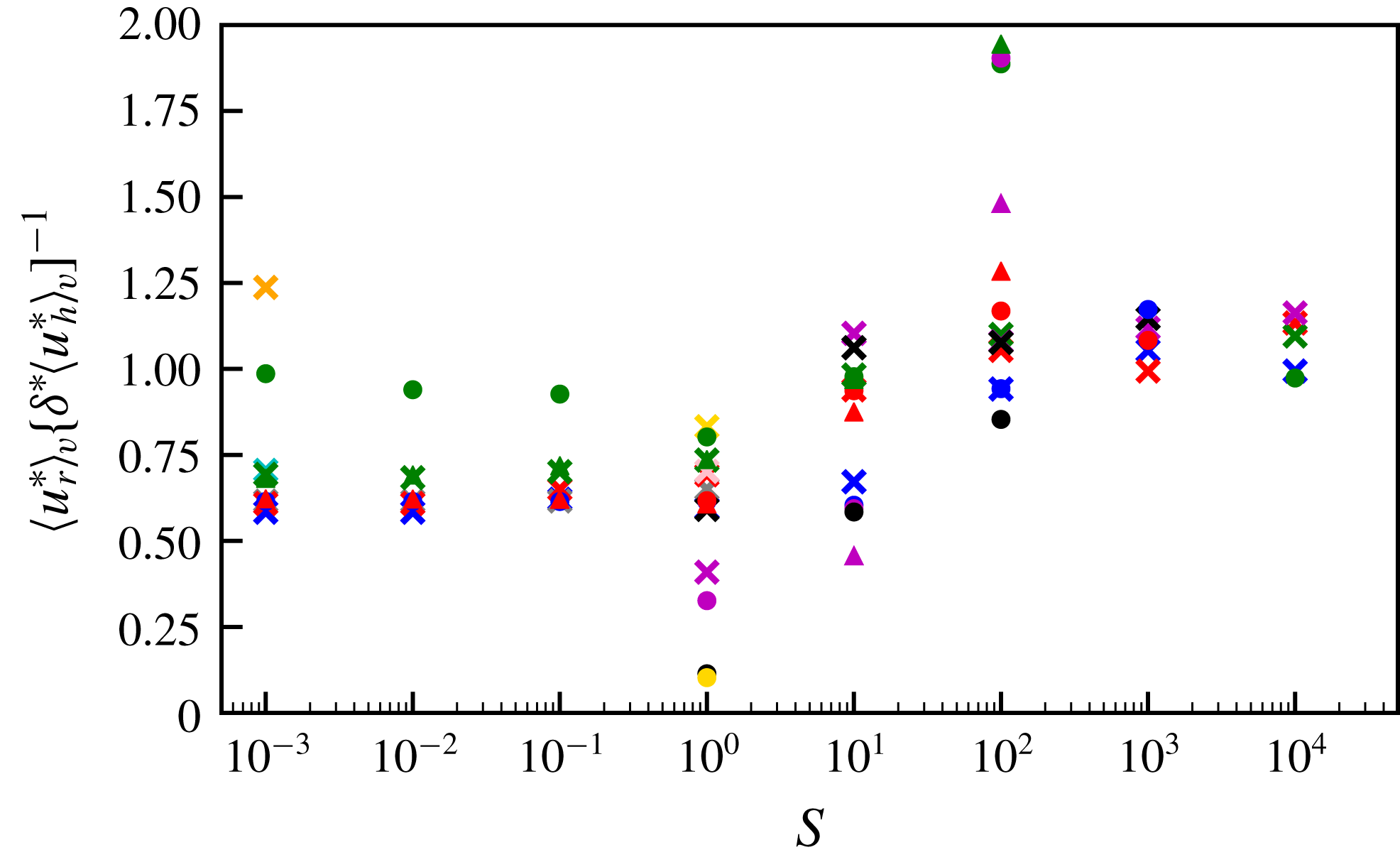
shown in figure 6. These results, summarised in figure 14 in appendix B, show clear flattening of
 $\langle u_{r}^{\ast }\rangle _{v}/\unicode[STIX]{x1D6FF}^{\ast }\langle u_{h}^{\ast }\rangle _{v}$
for the highest
 $S$
models, where
 $\langle u_{h}^{\ast }\rangle _{v}$
is the average volume-averaged horizontal velocity (
 $=[\langle u_{\unicode[STIX]{x1D703}}^{\ast }\rangle _{v}+\langle u_{\unicode[STIX]{x1D719}}^{\ast }\rangle _{v}]/2$
).
4.1.1 Vorticity equation balance
Taking the curl of (2.14) gives the dimensionless vorticity equation for steady flow
 $$\begin{eqnarray}\frac{\unicode[STIX]{x2202}\boldsymbol{u}^{\ast }}{\unicode[STIX]{x2202}z^{\ast }}=\unicode[STIX]{x1D735}\times BT_{1}^{\ast }\boldsymbol{r}^{\ast }+E\unicode[STIX]{x1D6FB}^{2}\unicode[STIX]{x1D74E}^{\ast },\end{eqnarray}$$
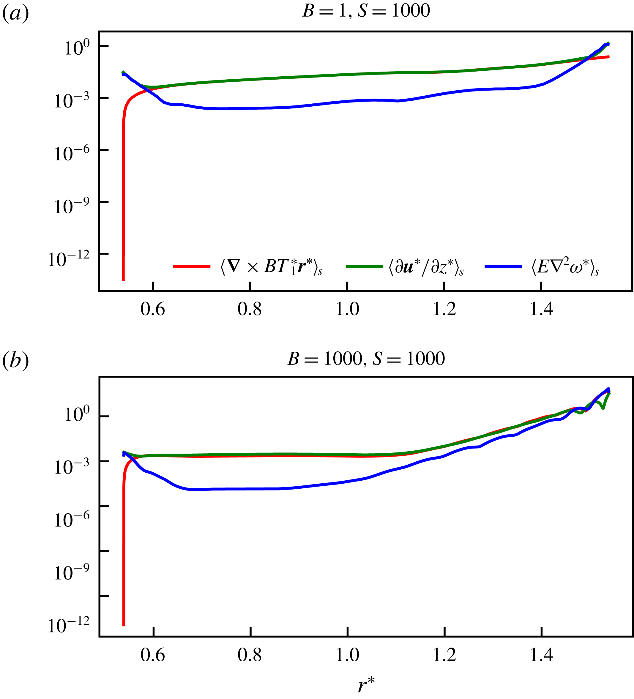
in which pressure does not appear and inertia is assumed small. In this three-term balance, we note that the buoyancy term is purely horizontal, and so the radial component of the first term must be small except outside the viscous boundary layer. Motivated by the observation that the viscous term is large only near the boundaries (see figure 15 in appendix B), we seek a thermal wind balance between the horizontal components of the Coriolis and buoyancy terms, and will show subsequently that the resulting scaling remains consistent for cases in which viscosity is also included in the balance.
We adopt
 $\unicode[STIX]{x1D6FF}^{\ast }$
as the relevant length scale in the Coriolis term that controls variations parallel to the rotation axis at high stratification (see figure 5), and an
 $O(1)$
horizontal length scale for the buoyancy term since it is determined by the boundary condition. The balance is then
 $$\begin{eqnarray}\frac{u_{\unicode[STIX]{x1D703},\unicode[STIX]{x1D719}}^{\ast }}{\unicode[STIX]{x1D6FF}^{\ast }}\sim BT_{1}^{\ast }.\end{eqnarray}$$
The volume-averaged magnitude of the Coriolis and buoyancy terms, scaled by our approximations to those terms using
 $\unicode[STIX]{x1D6FF}^{\ast }$
and volume-averaged velocities and temperatures (
 $\unicode[STIX]{x2202}\boldsymbol{u}^{\ast }/\unicode[STIX]{x2202}z^{\ast }\sim \langle u^{\ast }\rangle _{v}/\unicode[STIX]{x1D6FF}^{\ast }$
for Coriolis and
 $\unicode[STIX]{x1D735}\times BT_{1}^{\ast }\boldsymbol{r}^{\ast }\sim B\langle T_{f}^{\ast }\rangle _{v}$
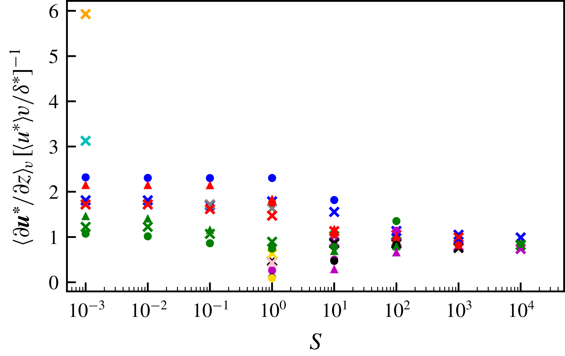
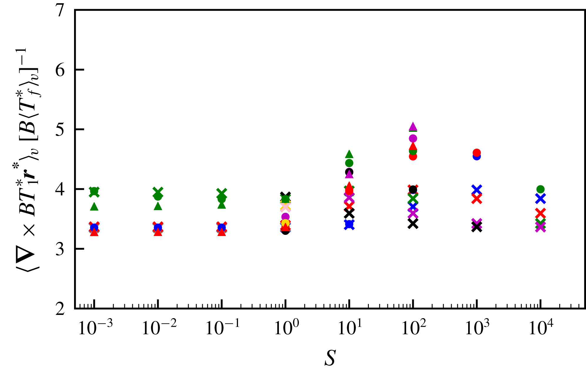
for buoyancy), are plotted for all models in figures 16 and 17 in appendix B. These ratios are approximately one for all high
 $S$
models, and show little
 $S$
dependence, indicating that the correct scalings are encapsulated in our approximations and that the volume-averaged quantities are suitable diagnostics of model output.
4.1.2 Temperature equation balance
The dimensionless time-independent temperature equation is
 $$\begin{eqnarray}\unicode[STIX]{x1D6FB}^{2}T_{1}^{\ast }-u_{r}^{\ast }\frac{\unicode[STIX]{x2202}T_{1}^{\ast }}{\unicode[STIX]{x2202}r^{\ast }}-\frac{u_{\unicode[STIX]{x1D703}}^{\ast }}{r}\frac{\unicode[STIX]{x2202}T_{1}^{\ast }}{\unicode[STIX]{x2202}\unicode[STIX]{x1D703}}-\frac{u_{\unicode[STIX]{x1D719}}^{\ast }}{r\sin \unicode[STIX]{x1D703}}\frac{\unicode[STIX]{x2202}T_{1}^{\ast }}{\unicode[STIX]{x2202}\unicode[STIX]{x1D719}}-Su_{r}^{\ast }r^{\ast }=0.\end{eqnarray}$$
Assuming that diffusion occurs on the length scale of the penetration depth, and that the geometric factors of
 $r$
and
 $\sin \unicode[STIX]{x1D703}$
are order unity, leaves
 $$\begin{eqnarray}\frac{T_{1}^{\ast }}{{\unicode[STIX]{x1D6FF}^{\ast }}^{2}}-3\frac{u_{r}^{\ast }}{\unicode[STIX]{x1D6FF}^{\ast }}T_{1}^{\ast }-Su_{r}^{\ast }\approx 0\end{eqnarray}$$
using the scaling for the velocity components of (4.2). The term
 $(\boldsymbol{u}^{\ast }\boldsymbol{\cdot }\unicode[STIX]{x1D735})T_{1}^{\ast }$
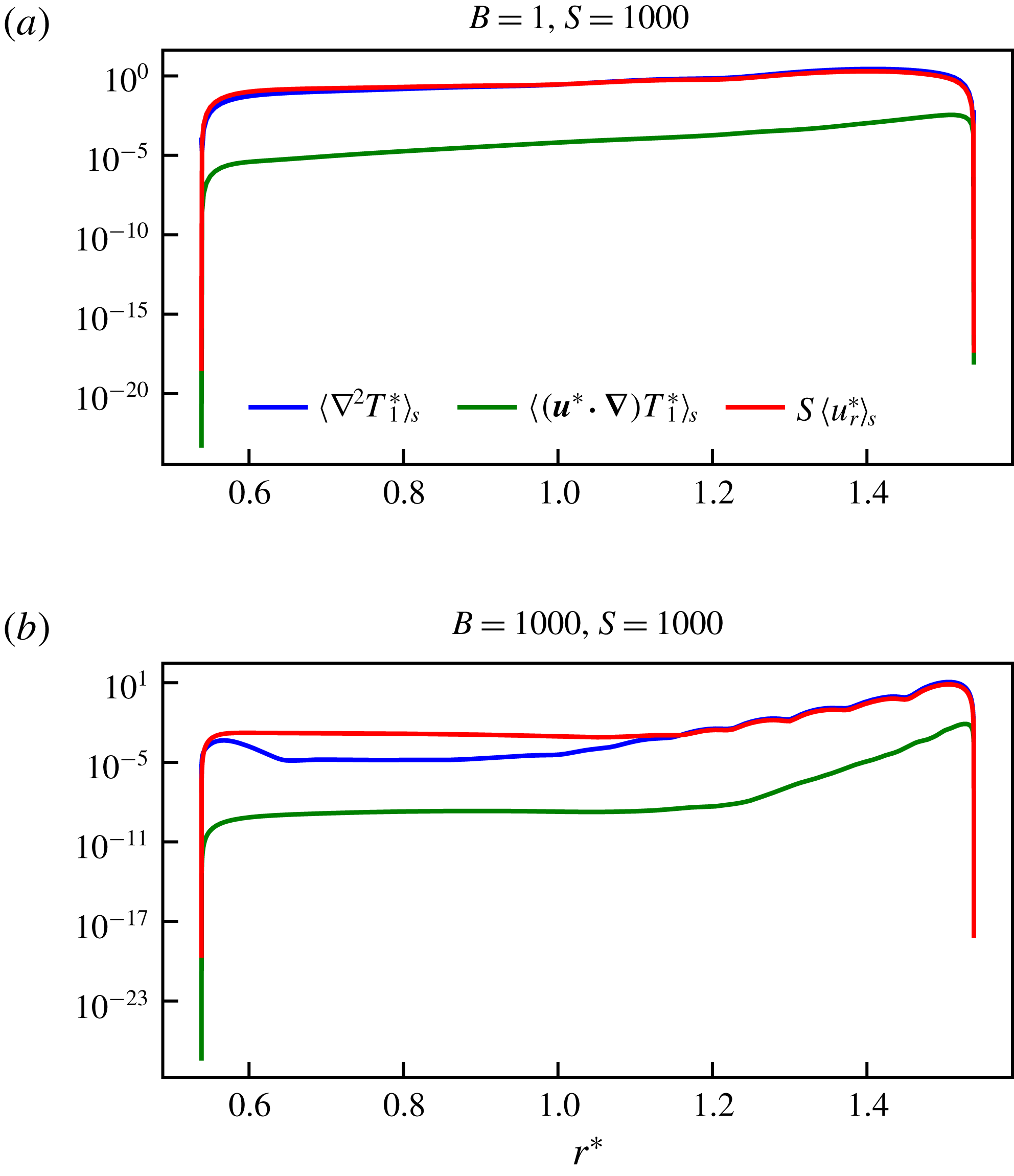
is small compared to the other terms (see figure 18 in appendix B for two representative high
 $S$
models). Therefore,
 $$\begin{eqnarray}\frac{T_{1}^{\ast }}{{\unicode[STIX]{x1D6FF}^{\ast }}^{2}}\sim Su_{r}^{\ast }\end{eqnarray}$$
is the appropriate balance. The approximation
 $\unicode[STIX]{x1D6FB}^{2}T_{1}^{\ast }\sim \langle T_{f}^{\ast }\rangle _{v}/{\unicode[STIX]{x1D6FF}^{\ast }}^{2}$
and the term balance in the temperature equation described by (4.7) were verified for our high
 $S$
models (see figure 19 in appendix B, which shows a clear flattening of
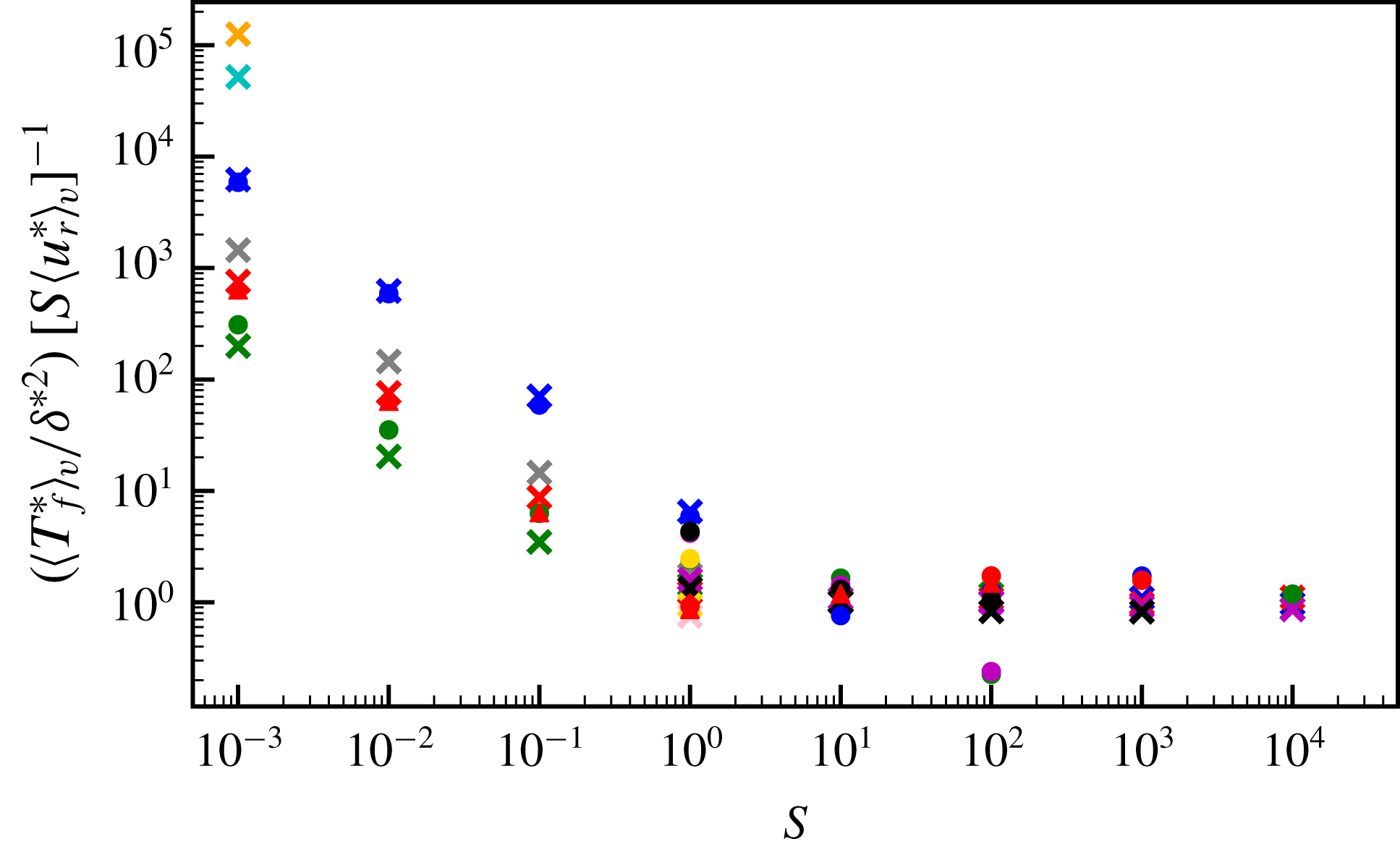
 $(\langle T_{f}^{\ast }\rangle _{v}/{\unicode[STIX]{x1D6FF}^{\ast }}^{2})/S\langle u_{r}^{\ast }\rangle _{v}$
for higher stratification parameters and little dependence on
 $B$
).
4.1.3 Power law scalings
Rearranging (4.7) for
 $\unicode[STIX]{x1D6FF}^{\ast }$
, eliminating
 $u_{r}^{\ast }$
using (4.2) from the continuity equation and substituting
 $BT_{1}^{\ast }\unicode[STIX]{x1D6FF}^{\ast }$
for horizontal flow (from balancing
 $\unicode[STIX]{x2202}\boldsymbol{u}^{\ast }/\unicode[STIX]{x2202}z^{\ast }$
with
 $\unicode[STIX]{x1D735}\times BT_{1}^{\ast }\boldsymbol{r}^{\ast }$
in (4.3)), results in a scaling for the penetration depth in terms of the control parameters
 $$\begin{eqnarray}\unicode[STIX]{x1D6FF}^{\ast }\sim (SB)^{-1/4}\sim (SRa_{{\mathcal{H}}}E)^{-1/4}.\end{eqnarray}$$
We now postulate that the radial velocity
 $u_{r}^{\ast }$
depends on
 $S$
but not
 $B$
as it is not directly forced by the thermal wind; it arises to conserve mass for the horizontal velocity components, which are directly forced by the boundary anomalies. Then
 $$\begin{eqnarray}u_{r}^{\ast }\sim S^{a},\end{eqnarray}$$
and the horizontal flow components scale as
 $$\begin{eqnarray}u_{\unicode[STIX]{x1D703},\unicode[STIX]{x1D719}}^{\ast }\sim S^{a+1/4}B^{1/4},\end{eqnarray}$$
from (4.2). The temperature perturbations depend on both
 $S$
and
 $B$
 $$\begin{eqnarray}T_{1}^{\ast }\sim S^{b}B^{c},\end{eqnarray}$$
where the exponents
 $b$
and
 $c$
are to be determined. From (4.7) and (4.8),
 $$\begin{eqnarray}S^{b-a}B^{c}\sim \frac{T_{1}^{\ast }}{u_{r}^{\ast }}\sim {\unicode[STIX]{x1D6FF}^{\ast }}^{2}S\sim S^{1/2}B^{-1/2},\end{eqnarray}$$
substituting (4.9) and (4.11), from which we deduce
 $c=-1/2$
and
 $b-a=1/2$
. Another assumption is required in order to proceed further with the analysis. We now assume that at sufficiently high
 $\unicode[STIX]{x1D6FD}$
, the boundary anomalies become unimportant so that the temperature perturbations are independent of
 ${\mathcal{H}}$
. Then,
 $T_{1}^{\ast }$
can only depend on the product
 $SB$
and, since the power of
 $B$
is
 $-1/2$
, the power of
 $S$
(
 $=b$
) must also be
 $-1/2$
. We have now determined the exponents for the temperature fluctuations
 $$\begin{eqnarray}T_{1}^{\ast }\sim (SB)^{-1/2}\sim (SRa_{{\mathcal{H}}}E)^{-1/2},\end{eqnarray}$$
radial flow
 $$\begin{eqnarray}u_{r}^{\ast }\sim S^{-1},\end{eqnarray}$$
and horizontal flow components
 $$\begin{eqnarray}u_{\unicode[STIX]{x1D703},\unicode[STIX]{x1D719}}^{\ast }\sim S^{-3/4}B^{1/4}\sim S^{-3/4}Ra_{{\mathcal{H}}}^{1/4}E^{1/4}.\end{eqnarray}$$
4.1.4 Empirical fit to models
In order to test the scaling laws obtained in the previous section, we computed best fits to our models using a least squares inversion of the estimates of the penetration depth and the volume-averaged velocities and temperature perturbations. We seek power laws of the form
 $$\begin{eqnarray}{\tilde{y}}=\unicode[STIX]{x1D716}S^{\unicode[STIX]{x1D712}}B^{\unicode[STIX]{x1D701}},\end{eqnarray}$$
where the ‘observations’
 $y$
are model outputs, and the predictions
 ${\tilde{y}}$
are calculated from the control parameters
 $S$
and
 $B$
, given the specified functional form. We take the logarithm to transform the power law problem into a linear problem such that
 $$\begin{eqnarray}\log {\tilde{y}}=\log \unicode[STIX]{x1D716}+\unicode[STIX]{x1D712}\log S+\unicode[STIX]{x1D701}\log B\end{eqnarray}$$
and calculate the prefactor
 $\unicode[STIX]{x1D716}$
and exponents
 $\unicode[STIX]{x1D712}$
and
 $\unicode[STIX]{x1D701}$
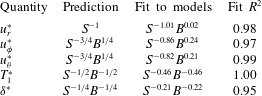
using a linear least squares inversion. A summary of the predicted scaling exponents ((4.8) and (4.13)–(4.15)) and those obtained from the least squares fits to all models in the stratification-dominated regime (
 $S>1$
) is provided in table 1 for comparison. A measure of how well the models are fit is given by the
 $R^{2}$
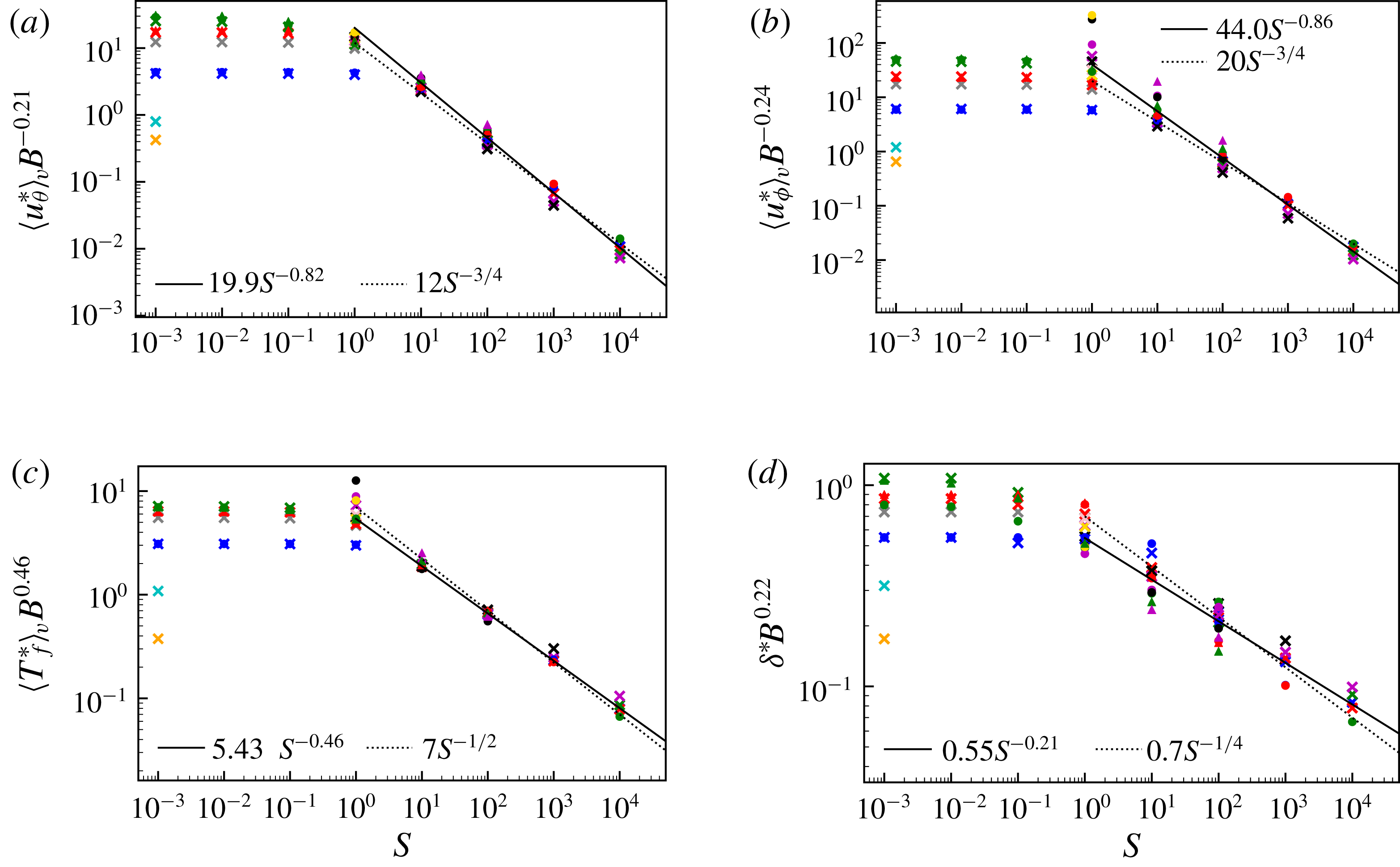
values (rounded to two decimal places throughout). The best fitting exponents are in good agreement with those obtained in the analysis; see also figures 9(a)–9(c).
(a) Volume-averaged meridional velocities, (b) volume-averaged azimuthal velocities, (c) volume-averaged temperature perturbations and (d) penetration depth estimates, normalised by the best empirical fit to the buoyancy parameter for all models with
 $S>1$
, as a function of
 $S$
. Symbol shapes represent the Ekman number,
 $E$
, and colours represent the buoyancy parameter,
 $B$
. The key is given in figure 6(a). The solid black lines show the best fitting power laws for
 $S$
in the stratification-dominated regime and the dotted lines show the theoretically predicted
 $S$
exponents.

Scaling analysis and least squares inversion results for all
 $S>1$
models.

4.1.5 The role of viscosity
Having verified our two-term balance in the vorticity equation, we now address the question of whether our scalings are also consistent when considering all three terms. The additional viscous term scales as
 $Eu^{\ast }\,l_{\unicode[STIX]{x1D708}}^{-3}$
, where
 $l_{\unicode[STIX]{x1D708}}$
is a relevant length scale yet to be determined.
The assertion that
 $l_{\unicode[STIX]{x1D708}}=\unicode[STIX]{x1D6FF}$
leads to
 $l_{\unicode[STIX]{x1D708}}=\unicode[STIX]{x1D6FF}\sim E^{1/2}$
independent of
 $S$
, which as figure 7 demonstrates is not the case as
 $\unicode[STIX]{x1D6FF}$
has clear empirical
 $S$
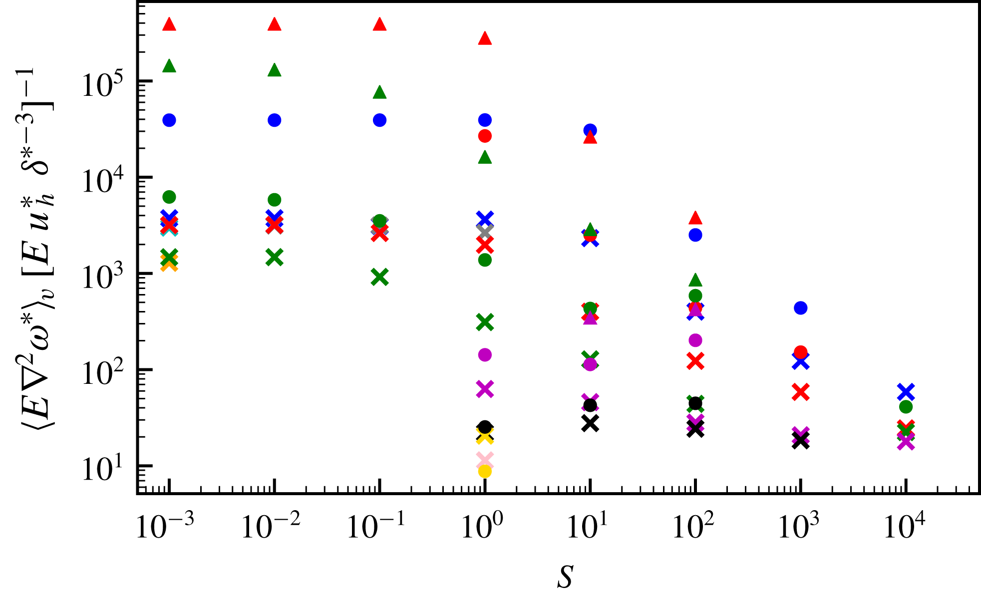
-dependence (see also figure 20 in appendix B, which shows the ratio of the viscous term to the incorrect scaling
 $Eu_{h}^{\ast }{\unicode[STIX]{x1D6FF}^{\ast }}^{-3}$
as a function of
 $S$
for all models). Alternatively, assuming that
 $l_{\unicode[STIX]{x1D708}}$
represents a thin boundary layer (consistent with figure 15), then the three-term balance determines
 $l_{\unicode[STIX]{x1D708}}$
to be
 $$\begin{eqnarray}l_{\unicode[STIX]{x1D708}}\sim (E\unicode[STIX]{x1D6FF}^{\ast })^{1/3}.\end{eqnarray}$$
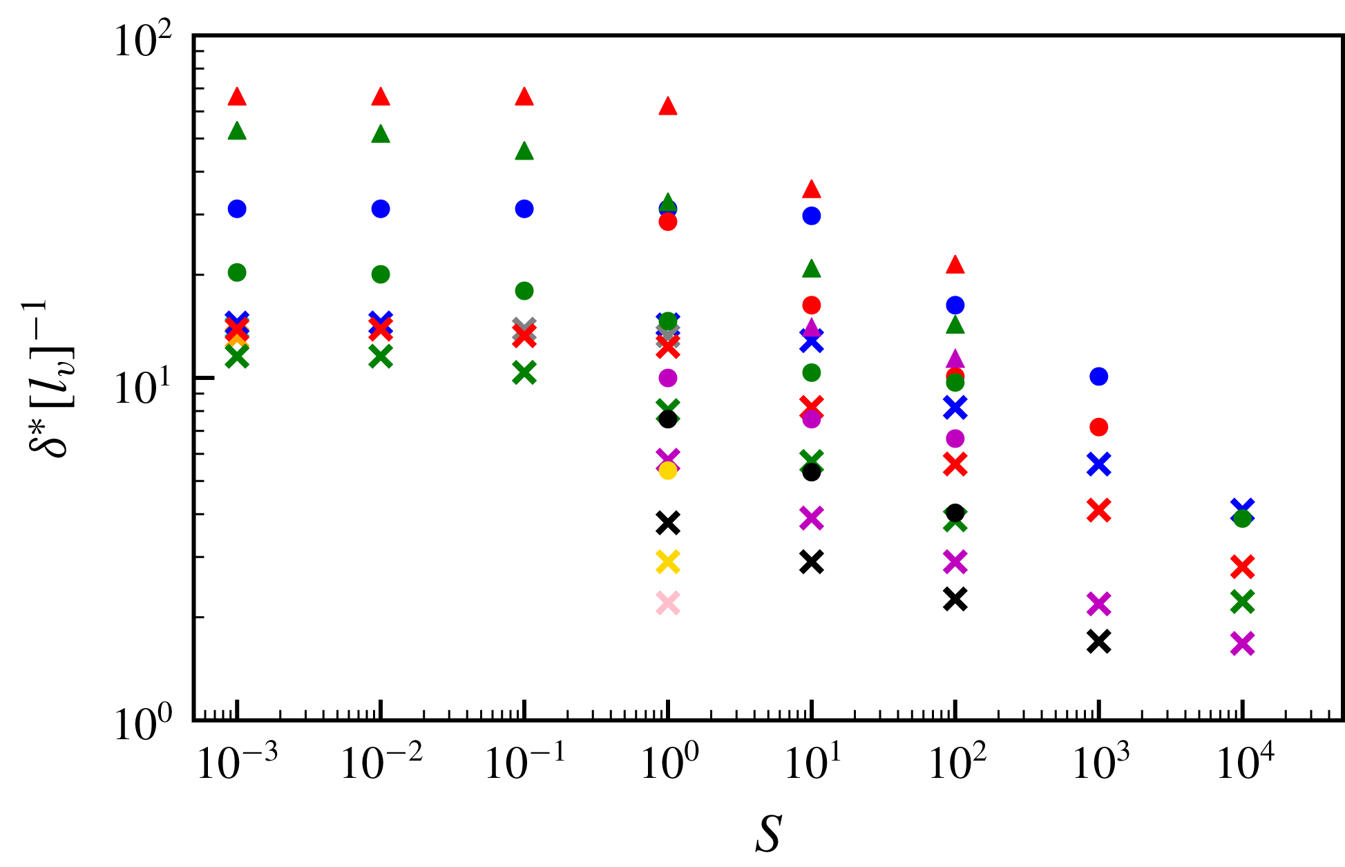
Figure 10 shows that the shear layer thickness (given in (4.8)) and the Ekman layer depth are comparable for most of our models, which are therefore in fact described by a three-term (rather than a two-term) balance within the shear layer. The inclusion of viscosity within the balance in no way invalidates our analysis of the two-term scaling, but merely provides information about the characteristic length scale
 $l_{\unicode[STIX]{x1D708}}$
at which viscosity becomes important. Indeed, our derived scalings of the previous sections, confirmed empirically, appear to hold independently of the relative size of
 $l_{\unicode[STIX]{x1D708}}$
and
 $\unicode[STIX]{x1D6FF}^{\ast }$
. It is worth pointing out the physically relevant planetary regime is one in which
 $E\ll 1$
and
 $l_{\unicode[STIX]{x1D708}}\ll \unicode[STIX]{x1D6FF}$
(see also § 5), and therefore in this limit the two-term balance is appropriate for the shear layer. We speculate that there may be a different behavioural regime in which
 $l_{\unicode[STIX]{x1D708}}\gg \unicode[STIX]{x1D6FF}^{\ast }$
for certain choices of parameters, when viscosity balances just one other term.
The shear layer thickness,
 $\unicode[STIX]{x1D6FF}^{\ast }$
, scaled by the dimensionless Ekman layer thickness estimated using (4.18) as a function of the stratification parameter,
 $S$
, for all steady models. Symbol shapes represent the Ekman number,
 $E$
, and colours represent the buoyancy parameter,
 $B$
. The key is given in figure 6(a).

4.2 Low stratification regime
At low
 $S$
, the basic state is one of neutral stability (rather than stratification) and the flow occupies the whole shell rather than being concentrated within a thin layer. Furthermore, from (2.12) it follows also that
 $T_{0}^{\ast }\approx 0$
so that
 $T^{\ast }\approx T_{1}^{\ast }$
. The dynamics of the low-
 $S$
regime has previously been investigated in Zhang & Gubbins (Reference Zhang and Gubbins1992), Gibbons & Gubbins (Reference Gibbons and Gubbins2000) and Gibbons et al. (Reference Gibbons, Gubbins and Zhang2007), but these studies did not develop scaling laws as we do here using a much broader range of models in
 $(E,S,B)$
space.
Within the low-
 $S$
regime, we consider the energy balance of (2.14) in a steady state, by taking the inner product with
 $\boldsymbol{u}^{\ast }$
and integrating over the volume
 $V$
. Neither the Coriolis force (which is orthogonal to the flow) nor the pressure contributes to the energy equation, as the fluid is incompressible and
 $$\begin{eqnarray}\int _{V}\boldsymbol{u}^{\ast }\boldsymbol{\cdot }\unicode[STIX]{x1D735}\hat{P}\,\text{d}V=\int _{V}\unicode[STIX]{x1D735}\boldsymbol{\cdot }(\hat{P}\boldsymbol{u}^{\ast })\,\text{d}V=0\end{eqnarray}$$
because
 $u_{r}^{\ast }=0$
on the boundary. The balance
 $$\begin{eqnarray}B\int _{V}T^{\ast }u_{r}^{\ast }r^{\ast }\,\text{d}V=E\int _{V}(\unicode[STIX]{x1D735}\times \boldsymbol{u}^{\ast })^{2}\,\text{d}V\end{eqnarray}$$
is then exact.
Following Shishkina, Grossmann & Lohse (Reference Shishkina, Grossmann and Lohse2016), the temperature equation (2.13) in steady state and the limit
 $S\rightarrow 0$
may be written
 $$\begin{eqnarray}\unicode[STIX]{x1D735}\boldsymbol{\cdot }(\boldsymbol{u}^{\ast }T^{\ast }-\unicode[STIX]{x1D735}T^{\ast })=0.\end{eqnarray}$$
Integrating over the volume bounded by radii
 $r^{\ast }$
and
 $r_{o}$
, with
 $r^{\ast }<r_{o}$
, and using the divergence theorem leads to
 $$\begin{eqnarray}\left\langle u_{r}^{\ast }T^{\ast }-\frac{\unicode[STIX]{x2202}T^{\ast }}{\unicode[STIX]{x2202}r^{\ast }}\right\rangle =0\end{eqnarray}$$
at any radius
 $r^{\ast }$
, where
 $\langle \cdot \rangle$
denotes integration over all solid angles, and where we have used the fact that both
 $u_{r}^{\ast }$
and
 $\langle \unicode[STIX]{x2202}T^{\ast }/\unicode[STIX]{x2202}r^{\ast }\rangle =\langle Y_{2}^{2}\rangle =0$
at
 $r^{\ast }=r_{o}$
. It follows that
 $$\begin{eqnarray}\int _{V}T^{\ast }u_{r}^{\ast }r^{\ast }\,\text{d}V=\int _{r_{i}}^{r_{o}}{r^{\ast }}^{3}\langle u_{r}^{\ast }T^{\ast }\rangle \,\text{d}r^{\ast }=\left\langle \int _{r_{i}}^{r_{o}}{r^{\ast }}^{3}\frac{\unicode[STIX]{x2202}T^{\ast }}{\unicode[STIX]{x2202}r^{\ast }}\,\text{d}r^{\ast }\right\rangle ,\end{eqnarray}$$
and integrating by parts leads to
 $$\begin{eqnarray}[\langle T^{\ast }\rangle ({r^{\ast }}^{3}-3{r^{\ast }}^{2}+6r^{\ast }-6)]_{r_{i}}^{r_{o}}=A(r_{o})\unicode[STIX]{x0394}T\end{eqnarray}$$
because
 $T^{\ast }=0$
on
 $r^{\ast }=r_{i}$
, where
 $A=r_{o}^{3}-3r_{o}^{2}+6r_{o}-6$
is a constant and
 $\unicode[STIX]{x0394}T=\langle T^{\ast }\rangle |_{r_{o}}$
. The exact relation
 $$\begin{eqnarray}BA\unicode[STIX]{x0394}T=E\int _{V}(\unicode[STIX]{x1D735}\times \boldsymbol{u}^{\ast })^{2}\,\text{d}V\end{eqnarray}$$
then follows. The viscous dissipation term on the right-hand side may be estimated as
 $(u^{\ast })^{2}$
by assuming a viscous boundary layer length scale of
 $E^{1/2}$
. The resulting scaling
 $$\begin{eqnarray}u^{\ast }\sim \sqrt{B\unicode[STIX]{x0394}T}\end{eqnarray}$$
is verified using an empirical fit to the low-
 $S$
models, which gives
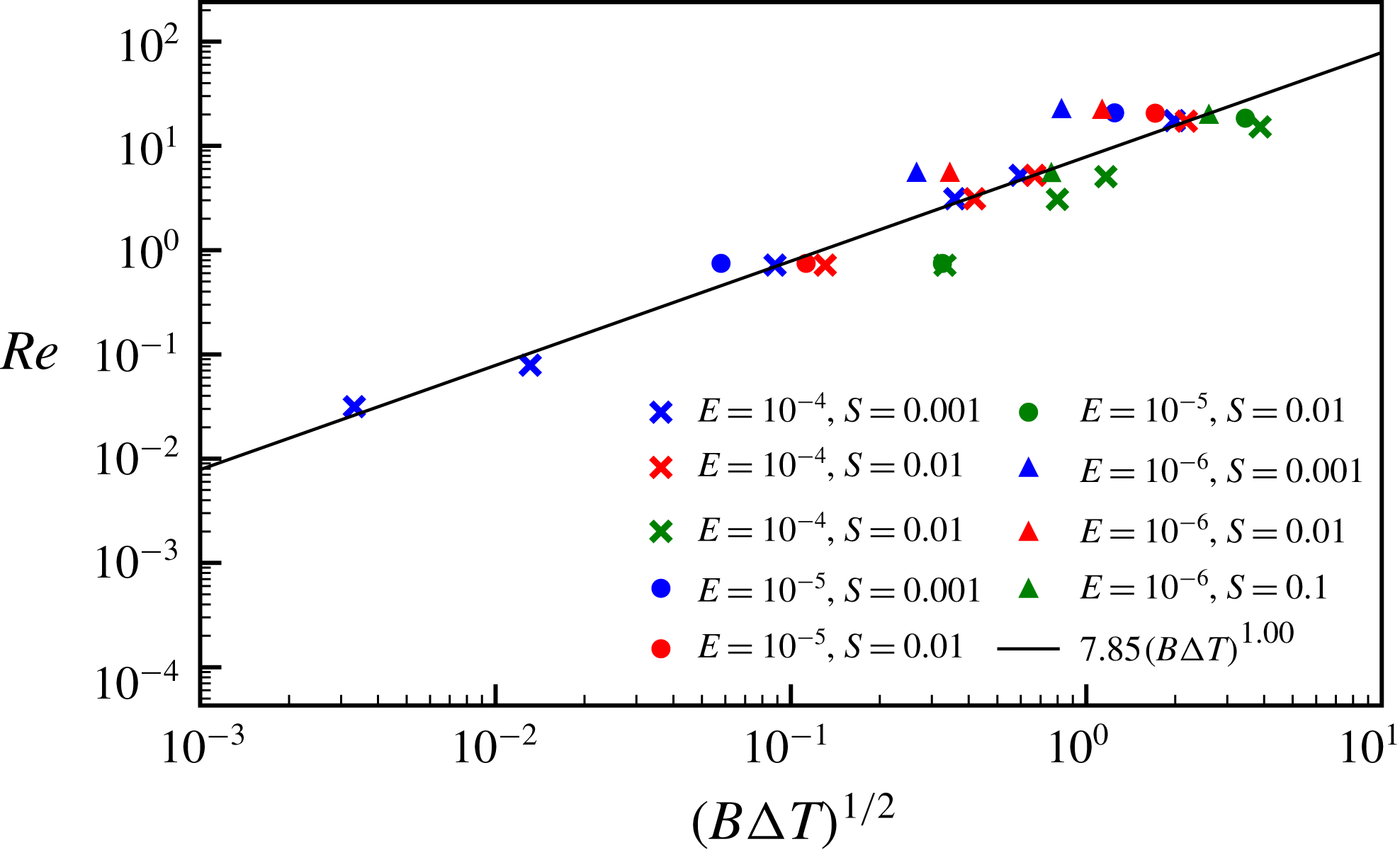
 $Re\sim (B\unicode[STIX]{x0394}T)^{0.50}$
(
 $R^{2}=0.88$
) and is shown in figure 11.
The Reynolds number
 $Re$
against
 $(B\unicode[STIX]{x0394}T)^{1/2}$
for all low-
 $S$
models. The black line shows the best empirical fit to the simulations.

We now need to estimate
 $\unicode[STIX]{x0394}T$
, which is not prescribed in models with a fixed heat-flux boundary condition, in contrast to those with a fixed temperature boundary condition. We consider the thermal dissipation equation, obtained by multiplying equation (2.13) with
 $T^{\ast }$
and integrating over
 $V$
:
 $$\begin{eqnarray}\int _{V}T^{\ast }\unicode[STIX]{x1D6FB}^{2}T^{\ast }\,\text{d}V=\frac{1}{2}\int _{V}(\boldsymbol{u}^{\ast }\boldsymbol{\cdot }\unicode[STIX]{x1D735}){T^{\ast }}^{2}\,\text{d}V=0\end{eqnarray}$$
since
 $u_{r}^{\ast }$
is zero on the boundaries, and so
 $$\begin{eqnarray}\left.\left\langle T^{\ast }\frac{\unicode[STIX]{x2202}T^{\ast }}{\unicode[STIX]{x2202}r^{\ast }}\right\rangle \right|_{r^{\ast }=r_{o}}=\int _{V}\unicode[STIX]{x1D735}\boldsymbol{\cdot }(T^{\ast }\unicode[STIX]{x1D735}T^{\ast })\,\text{d}V=-\int _{V}(\unicode[STIX]{x1D735}T^{\ast })^{2}\,\text{d}V\end{eqnarray}$$
because
 $T^{\ast }=0$
on the lower radial boundary. Since
 $\unicode[STIX]{x2202}T^{\ast }/\unicode[STIX]{x2202}r^{\ast }$
is prescribed as
 $Y_{2}^{2}$
on
 $r_{o}$
, this suggests the leftmost term is comparable to
 $\unicode[STIX]{x0394}T$
. In the rightmost term, we estimate
 $\unicode[STIX]{x1D735}T^{\ast }\sim \unicode[STIX]{x0394}T$
, which is reasonable if the majority of the dissipation occurs on the lateral length scale of
 $O(1)$
. Assuming that most of the dissipation occurs over a radial length scale
 $L_{T}$
at the top of the shell, the whole term is estimated to be
 $(\unicode[STIX]{x0394}T)^{2}L_{T}$
. Thus the balance in (4.28) is
 $\unicode[STIX]{x0394}T\sim (\unicode[STIX]{x0394}T)^{2}\,L_{T}$
or
 $$\begin{eqnarray}L_{T}\sim \unicode[STIX]{x0394}T^{-1}.\end{eqnarray}$$
Furthermore, balancing advection (which is dominated by horizontal gradients with length scales of
 $O(1)$
) and diffusion in the temperature equation (2.13) over the length scale
 $L_{T}$
leads to
 $u^{\ast }\sim L_{T}^{-2}$
. Hence
 $\unicode[STIX]{x0394}T\sim (u^{\ast })^{1/2}$
and it therefore follows that
 $$\begin{eqnarray}u^{\ast }\sim B^{2/3}\end{eqnarray}$$
and
 $$\begin{eqnarray}\unicode[STIX]{x0394}T\sim B^{1/3}.\end{eqnarray}$$
The scaling for
 $u^{\ast }$
is confirmed with an empirical fit to the low-
 $S$
simulations, which gives
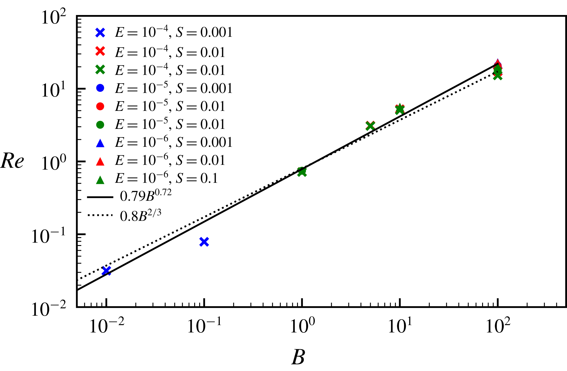
 $Re\sim B^{0.72}$
(
 $R^{2}=0.98$
) and is shown in figure 12. It is worth noting that the exponent (of
 $2/3$
) in the scaling for
 $u^{\ast }$
is higher than any of those reported in table 1 of Shishkina et al. (Reference Shishkina, Grossmann and Lohse2016) for the related study of plane layer horizontal convection with lateral temperature variations on the lower boundary.
The Reynolds number
 $Re$
against the buoyancy parameter
 $B$
for all low-
 $S$
models. The solid black line shows the best empirical fit to the simulations and the dotted line shows the theoretically predicted exponent from (4.30).

4.3 Effects of the shell aspect ratio
We have used an aspect ratio
 $\unicode[STIX]{x1D702}=0.35$
in all previous models, however as we would like to apply the derived scaling laws to other shells with different aspect ratios, we now consider whether varying the geometry influences the results. To this end, we have run simulations with
 $\unicode[STIX]{x1D702}=0.01$
using the parameters listed in table 6 and obtained steady-state solutions. It is apparent that the overall dynamics of the low aspect ratio models is very similar to the previously presented models, see figure 21 in appendix C. We again have two stratification regimes, a low
 $S$
regime in which the dynamics occupies the entire shell and buoyancy is the dominant effect, and a high
 $S$
regime in which stratification dominates and the dynamics is concentrated towards the outer boundary. In both regimes, the phase of the velocity and temperature lobes with respect to the boundary anomaly pattern is the same as in the previously discussed models. We have computed the best empirical fits to the high
 $S$
models in this geometry (shown in figure 13) and confirm that these models obey the same scaling laws as derived in 4.1.3. Note that the values of the quantities shown in figures 21 and 13, are different from those shown in previous sections for the same apparent parameter values because the length scales in the parameters
 $S$
and
 $B$
differ because
 $d=r_{o}-r_{i}=r_{o}(1-\unicode[STIX]{x1D702})$
, and averaging takes place over different volumes, meaning that for example,
 $B=1$
and
 $St=1000$
models at
 $\unicode[STIX]{x1D702}=0.35$
and
 $\unicode[STIX]{x1D702}=0.01$
are not directly comparable without accounting for geometric factors. It is worth remarking that the theoretical scaling for the horizontal velocity components (which scale as
 ${\sim}S^{-3/4}$
) actually agrees slightly better with the numerics in the quasi-full sphere than the spherical shell calculations, indicating a possible weak dependence on
 $r_{i}$
for such quantities.
(a) Volume-averaged radial velocities, (b) volume-averaged azimuthal velocities, (c) volume-averaged temperature perturbations and (d) penetration depth estimates, normalised by the best empirical fit to the buoyancy parameter for all models with
 $\unicode[STIX]{x1D702}=0.01$
and
 $S>1$
, as a function of
 $S$
. The
 $R^{2}$
values for the fits are, respectively, 0.95, 0.99, 1.00 and 0.99. Symbol shapes represent the Ekman number,
 $E$
, and colours represent the buoyancy parameter,
 $B$
. The black line shows the best fitting power law in
 $S$
for models at
 $S>1$
.

5 Application of scaling laws to planetary cores
In order to apply our power law scalings to a planet, we must estimate
 $S$
and
 $B$
for its outer core. We write
 $\unicode[STIX]{x1D6FD}$
and
 ${\mathcal{H}}$
in terms of temperature gradients at the CMB
 $$\begin{eqnarray}\unicode[STIX]{x1D6FD}\,d=\left.\frac{\text{d}T_{ad}}{\text{d}r}\right|_{r_{o}}-\left.\frac{\text{d}T_{c}}{\text{d}r}\right|_{r_{o}},\end{eqnarray}$$
where
 $T_{ad}$
is the adiabatic temperature and
 $T_{c}$
is the core temperature at the CMB, and
 $$\begin{eqnarray}{\mathcal{H}}=\left.\frac{\text{d}T^{\prime }}{\text{d}r}\right|_{r_{o}}=\frac{q^{\prime }}{k_{c}},\end{eqnarray}$$
where
 $T^{\prime }$
and
 $q^{\prime }$
are, respectively, the anomalous temperature and heat flow per unit area on the core side of the CMB. In (5.2), we have used the continuity of heat flux across the CMB along with its estimated value,
 $q^{\prime }$
, on the mantle side;
 $k_{c}$
is the thermal conductivity of the core. The gradients in (5.1) are evaluated using
 $$\begin{eqnarray}\left.\frac{\text{d}T_{ad}}{\text{d}r}\right|_{r_{o}}=-\frac{\unicode[STIX]{x1D6FC}_{T}g_{c}T_{c}}{C_{p}}\end{eqnarray}$$
and
 $$\begin{eqnarray}\left.\frac{\text{d}T_{c}}{\text{d}r}\right|_{r_{o}}=-\frac{Q_{cmb}}{A_{cmb}k_{c}},\end{eqnarray}$$
where
 $g_{c}$
is the acceleration due to gravity at the CMB,
 $C_{p}$
is the core specific heat,
 $Q_{cmb}$
is the total CMB heat flux,
 $A_{cmb}$
is the area of the CMB (
 $=4\unicode[STIX]{x03C0}r_{o}^{2}$
) and
 $k_{c}$
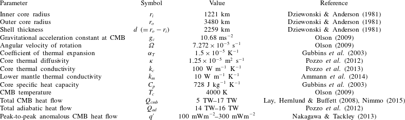
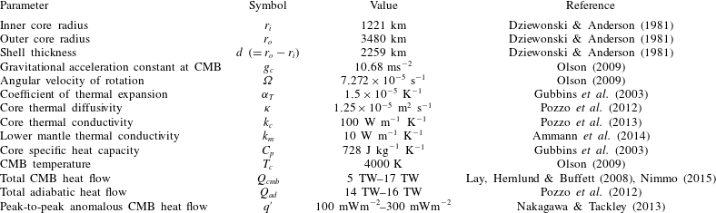
is the core thermal conductivity. For the Earth’s core, we have taken a range of plausible values from the literature, given in table 2, and calculated a range of possible
 $S$
and
 $B$
parameters. Estimating the stratification parameter (
 $S=\unicode[STIX]{x1D6FD}d/{\mathcal{H}}$
) is particularly challenging due to large uncertainties on
 ${\mathcal{H}}$
, the magnitude of lateral variations in CMB heat flux, whose estimate derives from relating observed shear-wave anomalies with either thermal or chemical heterogeneities. If the anomalies are attributed predominantly to thermal differences in the mantle, then the value of
 $q^{\prime }$
from table 2 leads to
 $S$
values of
 $O(10^{-6})$
–
 $O(10^{-4})$
and
 $B$
values of
 $O(10^{17})$
, placing the core in a regime in which the stratified layer is likely penetrated by unsteady boundary-driven flow.
Outer core and lower mantle physical, thermodynamic and transport properties used to estimate
 $S$
and
 $B$
for the Earth.
On the other hand, if the mantle heterogeneities are attributed instead to chemical anomalies (e.g. Garnero, McNamara & Shim Reference Garnero, McNamara and Shim2016; Lau et al.
Reference Lau, Mitrovica, Davis, Tromp, Yang and Al-Attar2017), then
 ${\mathcal{H}}$
could be much smaller than the above estimate, rendering
 $S$
plausibly
 $O(1)$
or above, placing the core in the stratification-dominated regime. Taking
 $S=1$
for illustration with our estimates of
 $B$
, applying the high
 $S$
scalings (4.13)–(4.15) gives dimensional temperature perturbations of
 $O(10^{-3}~\text{K})$
, radial velocities of
 $O(10^{-12}~\text{m}~\text{s}^{-1})$
, horizontal velocities of
 $O(10^{-7}~\text{m}~\text{s}^{-1})$
and penetration depths of approximately 70 m, much thicker than the estimated viscosity boundary layer in Earth’s core of approximately 1 m (e.g. Livermore, Bailey & Hollerbach Reference Livermore, Bailey and Hollerbach2016) associated with
 $E=10^{-15}$
. A similar analysis for Ganymede’s core, using values from table 1 of Rückriemen et al. (Reference Rückriemen, Breuer and Spohn2015) and estimating
 $\unicode[STIX]{x1D6FC}_{T}=5.8\times 10^{-5}$
based on Williams & Nimmo (Reference Williams and Nimmo2004), gives
 $B$
values of
 $O(10^{13})$
and
 $S$
values of
 $O(10^{-1})$
–
 $O(1)$
, assuming the mantle heterogeneities are attributed to thermal anomalies. As for the Earth, if the anomalies are predominantly due to chemical sources, these
 $S$
values are significantly underestimated and Ganymede’s core will be in the stratified regime.
For comparison with other works on stratified fluids, it is of interest to calculate the Brunt–Väisälä frequency,
 $N$
, defined by
 $$\begin{eqnarray}N^{2}=-\frac{g}{\unicode[STIX]{x1D70C}_{0}}\frac{\unicode[STIX]{x2202}\unicode[STIX]{x1D70C}^{\prime }}{\unicode[STIX]{x2202}r}\end{eqnarray}$$
both for our models and for the planetary interiors considered. Non-dimensionalising with the same scalings as used previously gives the ratio of the Brunt–Väisälä frequency to the rotation rate
 $$\begin{eqnarray}\frac{N}{2\unicode[STIX]{x1D6FA}}=\sqrt{\frac{BE}{Pr}\frac{\unicode[STIX]{x2202}T^{\ast }}{\unicode[STIX]{x2202}r^{\ast }}}=\sqrt{\frac{BES}{Pr}},\end{eqnarray}$$
assuming
 $\unicode[STIX]{x2202}T^{\ast }/\unicode[STIX]{x2202}r^{\ast }\approx \unicode[STIX]{x2202}T_{0}^{\ast }/\unicode[STIX]{x2202}r^{\ast }$
due to the small magnitudes of the temperature perturbations.
Values of this ratio for our simulations vary between
 $O(10^{-6})$
and
 $O(10)$
, given in tables 3–6 in appendix A. Based on our
 $B-S$
estimates for Earth and Ganymede, along with
 $E$
and
 $Pr$
estimates from table 1 of Schaeffer et al. (Reference Schaeffer, Jault, Nataf and Fournier2017) for Earth (
 $E=10^{-15}$
,
 $Pr=0.1-10$
) and table 4 of Schubert & Soderlund (Reference Schubert and Soderlund2011) for Ganymede (
 $E=10^{-13}$
,
 $Pr=0.1$
), we estimate their Brunt–Väisälä ratios of
 $O(1)$
for some parameter combinations, consistent with other estimates using different methods (e.g. Buffett Reference Buffett2014). Ignoring the dependence on
 $E$
, it is worth remarking that the relationship between
 $N$
and the product
 $S\,B$
may explain why this quantity is so important in our derived theoretical scalings, with
 $\unicode[STIX]{x1D6FF}^{\ast }\sim N^{-1/4}$
and
 $T_{1}^{\ast }\sim N^{-1/2}$
.
6 Discussion and conclusions
We have investigated a thermally stratified fluid in a rotating spherical shell subject to a laterally varying heat-flux pattern on the outer boundary. Converged, steady-state numerical simulations were obtained for
 $Pr=1$
,
 $E=10^{-6}$
to
 $E=10^{-3}$
,
 $S=10^{-3}$
to
 $S=10^{4}$
and
 $B=10^{-2}$
to
 $B=10^{6}$
. For some parameters, we obtained time-dependent solutions, which were not analysed in this study, however we were able to map the stability domain in parameter space in greater detail than any previous study. The steady-state solutions separate into two distinct dynamical regimes corresponding to low stratification parameter (
 $S$
), in which buoyancy effects dominate the dynamics, and high
 $S$
, in which stratification effects dominate.
In the low
 $S$
regime, the inhomogeneous thermal boundary condition drives flows that are locked to the boundary pattern and penetrate most of the shell thickness. We have developed scaling relationships for the characteristic velocity
 $Re$
and the temperature drop
 $\unicode[STIX]{x0394}T$
as a function of the buoyancy parameter
 $B$
. In the high
 $S$
regime, stratification strongly suppresses radial flow but horizontal flow is less affected. All flow is concentrated toward the outer boundary, resulting in shear layers whose thickness decreases with increasing
 $B$
and
 $S$
. This layer thickness represents the depth to which the boundary-driven flows penetrate the stratified fluid. We have developed scaling relations for the velocity components, temperature perturbations and penetration depth as functions of the control parameters
 $E$
,
 $B$
and
 $S$
; these are summarised in table 1. We have used these scaling relationships to extrapolate to Earth’s core using a range of plausible parameters. If the Earth’s mantle heterogeneities are attributed to thermal anomalies, the outer core is in the buoyancy-dominated regime and no steady-state solutions exist. In that case, it is likely that unsteady boundary-driven flows can penetrate the stratified layer. On the other hand, if such heterogeneities are linked to chemical anomalies (e.g. Garnero et al.
Reference Garnero, McNamara and Shim2016; Lau et al.
Reference Lau, Mitrovica, Davis, Tromp, Yang and Al-Attar2017), the much reduced heat-flux boundary condition would likely place Earth’s core in the stratification-dominated regime where penetration from steady boundary-driven flows is not possible. In that case, the shear layer thickness (i.e. the depth of penetration of boundary-driven flows through the core) is very small (of the order of a few tens of metres) compared to the stable layer thickness and the predicted velocities are several orders of magnitude smaller than those inferred from inversions of geomagnetic secular variation (e.g. Holme Reference Holme and Schubert2015). Since there is no reason why these inferred flows have to be generated (even in part) by mantle heterogeneities, the high
 $S$
scalings suggest that we infer general convective flow magnitudes rather than boundary-driven flow magnitudes from geomagnetic data. Furthermore, it seems unlikely that chemical anomalies in the lowermost mantle are able to directly affect the magnetic field that is generated inside the core (by creating persistent non-zonal features for example) through steady boundary-driven flows.
However, the relative contributions of thermal and chemical anomalies to the boundary forcing is poorly constrained for Earth and not at all for other bodies (including Ganymede), hence the difficulty in estimating
 ${\mathcal{H}}$
and the resulting uncertainty as to which stratification regime their outer cores belong. Interestingly, this means that independent evidence of penetrating flow within the stable layer, for example through the magnetic signature of upwellings and patches of reversed magnetic flux (Gubbins Reference Gubbins2007; Metman, Livermore & Mound Reference Metman, Livermore and Mound2018), may be able to discriminate between these two regimes and therefore offer evidence that constrains the heat flux on the boundary, and therefore mantle composition.
Finally, we have considered steady-state solutions in entirely stratified spherical shells with no convection or magnetic field generation; further work is needed to investigate the effects of adding these dynamics to our simplified models. The fluid dynamics problem studied here should be relevant in the uppermost region of the outer core, where no convection is expected due to stratification. Yet, it is possible that at sufficiently high
 $B$
, models at
 $S=1$
(the lowest stratification parameter required for our high
 $S$
scalings to be applicable, and a plausible value for Earth’s outer core) will be unsteady rather than steady. This transition may well occur at a
 $B$
lower than our estimates for Earth’s core, however, computational limitations have prevented us from reaching this transition and our simulations remain many orders of magnitude from Earth estimates. Since our systematic parameter study has revealed the different dynamical regimes that exist in the absence of internal convection, future studies will be able to benchmark against the present results and also target particular regions of parameter space to make most effective use of available computational resources.
Acknowledgements
We thank three anonymous referees for comments and suggestions that helped to improve the manuscript. This study was initiated by J.S. as his final year undergraduate project. G.A.C. was supported by NERC grant NE/M012190/1, and has received funding from Science Foundation Ireland grant 16/ERCD/4303 (iTHERC) and “3D Earth - A Dynamic Living Planet” funded by ESA as a Support to Science Element (STSE). C.J.D. is supported by a NERC Independent Research Fellowship (NE/L011328/1) and P.W.L. was partially supported by NERC grant NE/G014043/1. This work was undertaken on ARC2, part of the High Performance Computing facilities at the University of Leeds, UK. Contour plots were produced in VisIt (Childs et al. Reference Childs, Brugger, Whitlock, Meredith, Ahern, Bonnell, Miller, Weber, Harrison, Pugmire, Fogal, Garth, Sanderson, Bethel, Durant, Camp, Favrek, Rubel, Navrátil, Wheeler, Selby and Vivodtzev2012), using scripts written by J. Mound. Other figures were produced using Python’s Matplotlib (Hunter Reference Hunter2007).
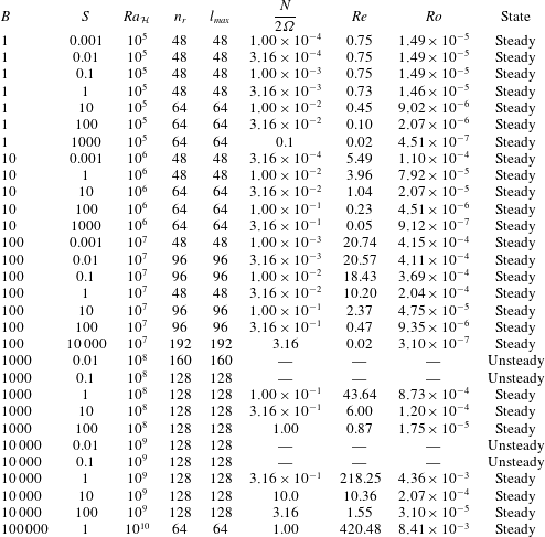
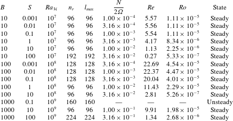
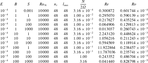
Appendix A. Summary tables
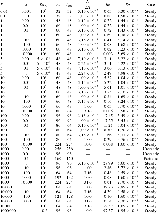
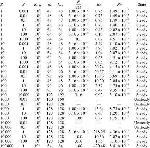
Summary tables of the model resolution, control parameters and selected output parameters for all simulations. In all cases
 $Pr=1$
and the shell aspect ratio
 $\unicode[STIX]{x1D702}=0.35$
for models in tables 3–5 and
 $\unicode[STIX]{x1D702}=0.01$
for models in table 6. Definitions for
 $B$
,
 $S$
and
 $Ra_{{\mathcal{H}}}$
are given in § 2.1. The quantity
 $N/2\unicode[STIX]{x1D6FA}$
, defined in (5.6), is the ratio of the Brunt–Väisälä frequency,
 $N$
, to the rotation rate
 $\unicode[STIX]{x1D6FA}$
. The variable
 $n_{r}$
is the number of radial points within the fluid shell,
 $l_{max}$
is the maximum degree of the spherical harmonic expansion (
 $=m_{max}$
, the maximum order of the expansion). Since
 $Re=Pe=\langle u^{\ast }\rangle _{v}$
, the Rossby number is
 $$\begin{eqnarray}Ro=2ReE=2\langle u^{\ast }\rangle _{v}E.\end{eqnarray}$$
Summary of all numerical simulations with
 $E=10^{-4}$
.
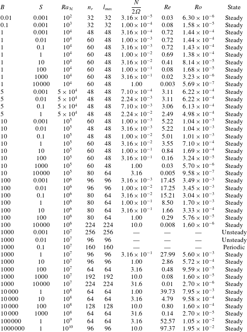
Summary of all numerical simulations with
 $E=10^{-5}$
.
Summary of all numerical simulations with
 $E=10^{-6}$
.

Summary of all numerical simulations with
 $E=10^{-4}$
and shell aspect ratio
 $\unicode[STIX]{x1D702}=0.01$
.

Radial velocity scaled by
 $\unicode[STIX]{x1D6FF}^{\ast }\langle u_{h}^{\ast }\rangle _{v}$
, where
 $\langle u_{h}^{\ast }\rangle _{v}$
is the average volume-averaged horizontal velocity, as a function of the stratification parameter,
 $S$
, for all steady models. Symbol shapes represent the Ekman number,
 $E$
, and colours represent the buoyancy parameter,
 $B$
. The key is given in figure 6(a).

All terms (denoted by line colour) in the dimensionless vorticity equation as a function of radius for two representative
 $E=10^{-4}$
models at high stratification parameter (
 $S=1000$
) and (a)
 $B=1$
and (b)
 $B=1000$
.

Volume-averaged Coriolis term of the vorticity equation (
 $\unicode[STIX]{x2202}\boldsymbol{u}^{\ast }/\unicode[STIX]{x2202}z^{\ast }$
), scaled by our approximation to that term (
 $\langle u^{\ast }\rangle _{v}/\unicode[STIX]{x1D6FF}^{\ast }$
), as a function of the stratification parameter,
 $S$
, for all steady models. Symbol shapes represent the Ekman number,
 $E$
, and colours represent the buoyancy parameter,
 $B$
. The key is given in figure 6(a).

Volume-averaged buoyancy term of the vorticity equation (
 $\unicode[STIX]{x1D735}\times BT_{1}^{\ast }\boldsymbol{r}^{\ast }$
), scaled by our approximation to that term (
 $B\langle T_{f}^{\ast }\rangle _{v}$
), as a function of the stratification parameter,
 $S$
, for all steady models. Symbol shapes represent the Ekman number,
 $E$
, and colours represent the buoyancy parameter,
 $B$
. The key is given in figure 6(a).

Appendix B. Scaling analysis figures
Figures 14–20 show examples of the term balances in the vorticity and temperature equations for a few representative high and low
 $S$
models. These figures are used to verify our scaling predictions (i.e. that we have used the correct length scales in various terms) and to justify only considering certain terms in the governing equation in the scaling analyses, as they make clear that the balances we consider are both applicable in our two
 $S$
regimes, appropriately scaled in our analysis and that our volume-averaged model diagnostics are appropriate (as we could have chosen other diagnostic outputs from the simulations).
All terms (denoted by line colour) in the dimensionless temperature equation as a function of radius for two representative
 $E=10^{-4}$
models at high stratification parameter (
 $S=1000$
) and (a)
 $B=1$
and (b)
 $B=1000$
.

Ratio of the two dominant terms in the temperature equation as a function of the stratification parameter,
 $S$
, for all steady models. Symbol shapes represent the Ekman number,
 $E$
, and colours represent the buoyancy parameter,
 $B$
. The key is given in figure 6(a).

Volume-averaged viscous term of the vorticity equation (
 $E\unicode[STIX]{x1D6FB}^{2}\unicode[STIX]{x1D714}^{\ast }$
), scaled by the (incorrect) approximation to that term (
 $Eu_{h}^{\ast }{\unicode[STIX]{x1D6FF}^{\ast }}^{-3}$
), as a function of the stratification parameter,
 $S$
, for all steady models. Symbol shapes represent the Ekman number,
 $E$
, and colours represent the buoyancy parameter,
 $B$
. The key is given in figure 6(a).

Appendix C. Low shell aspect ratio dynamics
Figure 21 shows the effects on the dynamics of low aspect ratio models.
Equatorial plots of
 $T_{f}^{\ast }$
(a,b),
 $u_{r}^{\ast }$
(c,d) and
 $u_{\unicode[STIX]{x1D719}}^{\ast }$
(e,f) for models with shell aspect ratio
 $\unicode[STIX]{x1D702}=0.01$
at
 $E=10^{-4}$
,
 $B=1$
and
 $S=0.001$
(a,c,e) and 1000 (b,d,f). Red indicates positive values and blue indicates negative values. Note the different colour scales. Locations of high (H) and low (L) outward heat flux are shown on the top left.