


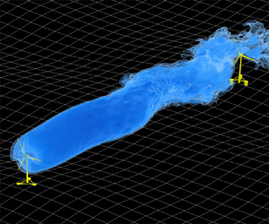

1. Introduction
As a wind turbine extracts kinetic energy from the atmospheric boundary layer, it leaves behind a wake with low speed and high turbulence intensity (TI) (Vermeer, Sørensen & Crespo Reference Vermeer, Sørensen and Crespo2003). Wakes reduce the power and increase the fatigue load of downstream wind turbines in large wind farms and are responsible for a loss of over 10 % of annual energy production (Barthelmie et al. Reference Barthelmie2009). A profound understanding of the fluid mechanics underlying the wake evolution is thus indispensable for farm-level optimization of power production and has become a focus for both the wind energy and fluid mechanics community (Stevens & Meneveau Reference Stevens and Meneveau2017; Porté-Agel, Bastankhah & Shamsoddin Reference Porté-Agel, Bastankhah and Shamsoddin2020; Shapiro, Starke & Gayme Reference Shapiro, Starke and Gayme2022). The major challenge is related to the wake's high Reynolds number and the complex interaction between the wind turbine wakes and the atmospheric boundary layer (Veers et al. Reference Veers2019; Meyers et al. Reference Meyers, Bottasso, Dykes, Fleming, Gebraad, Giebel, Göçmen and van Wingerden2022).
For floating offshore wind turbines (FOWTs), the degrees of freedom of the platform motion further complicate the wake-turbine interaction in a two-way manner. On the one hand, the motion of the FOWT can be intensified by the wake-induced unsteady aerodynamic load (Wise & Bachynski Reference Wise and Bachynski2020). On the other hand, the motion of the FOWT can substantially enhance the unsteadiness in the far wake by triggering large-scale coherent turbulent structures (Li, Dong & Yang Reference Li, Dong and Yang2022; Messmer, Hölling & Peinke Reference Messmer, Hölling and Peinke2023) that may affect the load and performance of downstream neighbours. In this paper we propose a linearized wake model based on the resolvent of the linearized Navier–Stokes equation (LNSE), which can be solved by a personal computer within several minutes for each simple harmonic motion, such that these coherent turbulent structures can be predicted efficiently.
The wake of FOWTs has received research attention in the fields of fluid mechanics, wind energy and ocean engineering over the past decade. Special influences of FOWT motion were initially identified in the near wake in studies focusing on unsteady blade aerodynamics (Sebastian & Lackner Reference Sebastian and Lackner2012; Farrugia, Sant & Micallef Reference Farrugia, Sant and Micallef2016; Tran & Kim Reference Tran and Kim2016; Fontanella et al. Reference Fontanella, Bayati, Mikkelsen, Belloli and Zasso2021), where the breakdown of the tip vortices was found to be accelerated by FOWT motions. At a floating wind farm level, the focus is shifted to the motion-induced wake evolution at a larger downstream distance, using numerical simulations (Lee & Lee Reference Lee and Lee2019; Kopperstad, Kumar & Shoele Reference Kopperstad, Kumar and Shoele2020; Chen, Liang & Li Reference Chen, Liang and Li2022; Li et al. Reference Li, Dong and Yang2022; Kleine et al. Reference Kleine, Franceschini, Carmo, Hanifi and Henningson2022; Ramos-García et al. Reference Ramos-García, González Horcas, Pegalajar-Jurado, Kontos and Bredmose2022), wind tunnel experiments with wind turbine models (Rockel et al. Reference Rockel, Camp, Schmidt, Peinke, Cal and Hölling2014, Reference Rockel, Peinke, Hölling and Cal2017; Bayati et al. Reference Bayati, Belloli, Bernini and Zasso2017; Fu et al. Reference Fu, Jin, Zheng and Chamorro2019; Schliffke, Aubrun & Conan Reference Schliffke, Aubrun and Conan2020; Feist, Sotiropoulos & Guala Reference Feist, Sotiropoulos and Guala2021; Belvasi et al. Reference Belvasi, Conan, Schliffke, Perret, Desmond, Murphy and Aubrun2022; Meng et al. Reference Meng, Su, Qu and Lei2022b; Messmer et al. Reference Messmer, Hölling and Peinke2023) and field measurement with a full-scale FOWT (Angelou, Mann & Dubreuil-Boisclair Reference Angelou, Mann and Dubreuil-Boisclair2023). Despite variations in the environmental settings, turbine sizes and motion types, these studies achieve some consensus on the far wake evolution of a FOWT, which are synthesized in the following.
(i) Motion-specific. Most studies focus on the fore–aft motion, i.e. surge and pitch. The wind tunnel experiments of Fontanella et al. (Reference Fontanella, Bayati, Mikkelsen, Belloli and Zasso2021); Fontanella, Zasso & Belloli (Reference Fontanella, Zasso and Belloli2022) reveal that surge motion induces a thrust variation and generates oscillations of the axial wake velocity at the same frequency of the imposed motion, based on measurements located at 2.3 times the rotor diameter downstream of the wind turbine. Interestingly, this near wake velocity fluctuation may further develop into a pulsing mode featured by alternating wind speed variation in the streamwise direction and a varicose deformation in the far wake (Kopperstad et al. Reference Kopperstad, Kumar and Shoele2020). On the other hand, the side-to-side motion, i.e. sway and roll, is found to trigger wake meandering characterized by the wake's oscillatory displacement in the lateral direction (Fu et al. Reference Fu, Jin, Zheng and Chamorro2019; Meng et al. Reference Meng, Su, Qu and Lei2022b), which is locked at the motion frequency and its multiples (Li et al. Reference Li, Dong and Yang2022). Moreover, this wake meandering induced by the side-to-side motion is found to trigger a faster wake recovery (Li et al. Reference Li, Dong and Yang2022) than the surge motion (Schliffke et al. Reference Schliffke, Aubrun and Conan2020). Recent experiments by Messmer et al. (Reference Messmer, Hölling and Peinke2023) indicate that if the surge motion falls in a specific frequency range, wake meandering can also be triggered through a nonlinear mechanism (Gupta & Wan Reference Gupta and Wan2019).
(ii) Frequency-dependent. Since the shear layer and the helical vortices of wind turbine wakes are unstable and have different sensitive frequencies (Iungo et al. Reference Iungo, Viola, Camarri, Porté-Agel and Gallaire2013; Mao & Sørensen Reference Mao and Sørensen2018; Gupta & Wan Reference Gupta and Wan2019; Kleine et al. Reference Kleine, Franceschini, Carmo, Hanifi and Henningson2022), the wind turbine wake's response changes significantly as the frequency of the FOWT motion varies. The Strouhal number is often employed as the characteristic non-dimensional number for the frequency, which is defined as
 $St= \omega D/ (2 {\rm \pi}U_{\infty })$, with $\omega$ the angular frequency, $D$ the rotor diameter and $U_\infty$ the free-stream wind speed. The instability of the wake is found to be less pronounced and the wake response is quasi-steady at small $St$. One example is the experiment by Meng et al. (Reference Meng, Su, Qu and Lei2022b), which found that a sway motion at $St<0.01$ with a rather large amplitude $A = 0.2D$ only led to a wake offset near the rotor with an amplitude close to the motion. When increasing the motion frequency, the instability related to the shear layer of the wake can amplify the motion-induced perturbation and develop in the far wake. An example is the large-eddy simulation (LES) of Li et al. (Reference Li, Dong and Yang2022), which showed that the sway motion at $St=0.25$ led to large far wake meandering even with a small initial motion amplitude $A = 0.01D$. The study further employed linear stability analysis (LSA) and LES to find a sensitive range of $0.2< St<0.6$, in which the sway motion triggers large wake meandering and enhances the wake recovery. These results are confirmed by a recent wind tunnel experiment by Messmer et al. Reference Messmer, Hölling and Peinke2023. Besides, the experiment by Messmer et al. (Reference Messmer, Hölling and Peinke2023) discovers a novel nonlinear phenomenon caused by surge motions with $0.6< St<0.9$, which not only leads to the pulsing mode at the forcing frequency but also results in lateral wake meandering at lower frequencies. For higher motion frequencies, the analysis of Kleine et al. (Reference Kleine, Franceschini, Carmo, Hanifi and Henningson2022) demonstrates that motions at 1.5 times the rotor frequency induces the strongest disturbances to the tip vortices in the near wake.
(iii) Sensitive to ambient turbulence. The stability of free shear layers (wake, jet, mixing layer, etc) is known to be sensitive to inflow turbulence (Ho & Huerre Reference Ho and Huerre1984). However, motion-induced wake evolution is often investigated with uniform inflows (Chen et al. Reference Chen, Liang and Li2022; Kleine et al. Reference Kleine, Franceschini, Carmo, Hanifi and Henningson2022) or with very low TIs (Meng et al. Reference Meng, Su, Qu and Lei2022b). The LES of Li et al. (Reference Li, Dong and Yang2022) shows that the meandering induced by the rotor sway motion is inversely related to the inflow TIs, such that the meandering amplitude increases when the inflow TI is decreased, being exactly opposite to the trend for the wake meandering of fixed wind turbines with turbulent inflows (Espana et al. Reference Espana, Aubrun, Loyer and Devinant2012; Yang & Sotiropoulos Reference Yang and Sotiropoulos2019). For cases with sufficiently high TI, the wakes of a wind turbine with and without sway motion are found to be similar (Li et al. Reference Li, Dong and Yang2022). This phenomenon is also observed in the wind tunnel experiment by Belvasi et al. (Reference Belvasi, Conan, Schliffke, Perret, Desmond, Murphy and Aubrun2022), indicating no obvious motion-enhanced wake recovery with an inflow TI = 8 %. However, at low to intermediate intensities, the interplay between the rotor motion with the free-stream turbulence is yet to be fully understood.


In summary, the existing research has shown that the wake of a FOWT responds actively to the platform motion at low TIs (Kleine et al. Reference Kleine, Franceschini, Carmo, Hanifi and Henningson2022; Li et al. Reference Li, Dong and Yang2022; Messmer et al. Reference Messmer, Hölling and Peinke2023). It is found that certain motion types falling in a specific frequency range of the shear layer instability can lead to wind speed fluctuation in the far wake and enhance the wake recovery (Li et al. Reference Li, Dong and Yang2022; Messmer et al. Reference Messmer, Hölling and Peinke2023). While the LSA of the shear layer was shown to be able to estimate the sensitive frequency range (Gupta & Wan Reference Gupta and Wan2019; Li et al. Reference Li, Dong and Yang2022), it is not yet possible to predict the wake response for a specific motion. There are two reasons for this shortcoming. Firstly, the LSA focuses on the property of the shear layer itself and formulates an eigenvalue problem without considering a specific external perturbation. Secondly, the concrete form of the initial perturbation caused by FOWT motions to the shear layer of the wake is neither well understood. Recently, Kleine et al. (Reference Kleine, Franceschini, Carmo, Hanifi and Henningson2022) studied the effect of FOWT motion on the near wake tip vortices, but the effect of such motions on the shear layer and far wake evolution was not considered.
In this work we propose a linear and deterministic model that predicts the far wake evolution induced by specific rotor motions, as depicted by figure 1. The proposed model consists of two parts, i.e. a forcing-to-wake (F2W) part and a motion-to-forcing (M2F) part. The first part is designed to transfer arbitrary forcing on the rotor into the wake response by establishing a bi-global resolvent model of the wake that reflects the stability property of the wake shear layer. The latter part, i.e. the M2F model, equates the motion of the wind turbine to a set of motion-specific unsteady aerodynamic forces. When used separately, the F2W model can predict the optimal forcing at the rotor for triggering the strongest far wake response. Combining both models predicts the wake response in an end-to-end and motion-specific manner. In addition to this model, the influence of ambient turbulence on a FOWT's wake will be further investigated using LES, considering both the effect of the inflow TI and the turbulence length scale, within a low to intermediate TI condition ( $2.5\,\% \le {\rm TI} \le 7.5\,\%$). The predictive ability of the proposed model will be evaluated in both uniform and turbulent inflow conditions. To the best of the authors’ knowledge, no linearized model has been proposed to achieve such a global and motion-specific prediction for FOWT's wakes. As a first step, the model proposed in the present paper assumes a non-sheared inflow and an axisymmetric wind turbine wake.
Structure of the proposed motion-to-wake model of floating wind turbine wakes.

The remainder of this paper is structured as follows. Section 2 presents the numerical methods and the set-ups of LES cases carried out in this study. The simulation results of the wake for FOWT undergoing different motions are presented in § 3 with a uniform inflow. In § 4 the proposed motion-to-wake (M2W) modelling is derived and validated against LES results. Section 5 investigates the effects of free-stream turbulence on the motion-induced wake meandering through LES, and proposes an extension of the M2W model to incorporate these effects. Finally, a conclusion is provided at the end of the paper.
2. Large-eddy simulation method and case configuration
2.1. Numerical method
The nonlinear evolution of wind turbine wake is simulated with the VFS-Wind code (Yang et al. Reference Yang, Sotiropoulos, Conzemius, Wachtler and Strong2015), assuming the air is a Newtonian fluid with a constant density and viscosity. The flow is governed by the filtered incompressible Navier–Stokes equations, written in Cartesian coordinates as
 \begin{gather} \boldsymbol{\nabla} \boldsymbol{\cdot} \tilde{\boldsymbol{u}} = 0 , \end{gather}
 \begin{gather}\frac{\partial \tilde{\boldsymbol{u}}}{\partial t}+(\tilde{\boldsymbol{u}} \boldsymbol{\cdot} \boldsymbol{\nabla}) \tilde{\boldsymbol{u}} ={-}\boldsymbol{\nabla} \tilde{p} + \nu {\nabla}^2 \tilde{\boldsymbol{u}} - \boldsymbol{\nabla} \boldsymbol{\cdot} \boldsymbol{\tau} + \boldsymbol{f}, \end{gather}
where  $\boldsymbol {u} = \{u_x, u_y, u_z\}$ is the velocity vector in the Cartesian coordinates,
 $p$ is the pressure and
 $\nu$ is the fluid kinematic viscosity. Here
 $\tilde {{\cdot }}$ denotes the spatial filtering process;
 $\boldsymbol {\tau }$ is the subgrid-scale stress resulting from the filtering of the nonlinear convection term and is closed with the dynamic Smagorinsky model (Smagorinsky Reference Smagorinsky1963; Germano et al. Reference Germano, Piomelli, Moin and Cabot1991);
 $\boldsymbol {f}$ denotes the body force term. In the equation, bold symbols represent vectors (e.g.
 $\boldsymbol {u}$) or two-dimensional tensors (e.g.
 $\boldsymbol {\tau }$), the rest are scalar variables.
In wind turbine wake simulations the body force term  $\boldsymbol {f}$ represents the effect of wind turbines on the flow and is computed using a well-validated actuator surface model (Yang & Sotiropoulos Reference Yang and Sotiropoulos2018) for both the rotor and nacelle. This model simplifies each rotor blade as a zero-thickness rotating surface that exerts aerodynamic forces on the surrounding flow. The aerodynamic forces on each blade element are computed individually using two-dimensional blade aerodynamic coefficients as
 \begin{gather} \boldsymbol{F} = \boldsymbol{L} + \boldsymbol{D}, \end{gather}
 \begin{gather} \boldsymbol{L} = \tfrac{1}{2}c C_{L}(\alpha, Re_c)|V_{ref}|^2 \boldsymbol{e_{L}}, \end{gather}
 \begin{gather} \boldsymbol{D} = \tfrac{1}{2}c C_{D}(\alpha, Re_c)|V_{ref}|^2 \boldsymbol{e_{D}}, \end{gather}
where  $\boldsymbol {F}$ is the aerodynamic force per unit span, with
 $\boldsymbol {L}$ and
 $\boldsymbol {D}$ the lift and drag coefficients. Here
 $C_L(\alpha, Re_c)$ and
 $C_D(\alpha, Re_c)$ are the lift and drag coefficients, depending on the local airfoil and the angle of attack (
 $\alpha$) and the Reynolds number (
 $Re_c$) defined with the chord length (
 $c$);
 $V_{ref}$ is the relative flow velocity with respect to the rotating blade;
 $\boldsymbol {e}_{L}$ and
 $\boldsymbol {e}_{D}$ are unit vectors defining the lift and drag directions. Three-dimensional effects (Du & Selig Reference Du and Selig1998) and the tip loss (Shen et al. Reference Shen, Mikkelsen, Sørensen and Bak2005) are corrected before computing the momentum source in (2.2)
 \begin{equation} \boldsymbol{f} = \boldsymbol{F}/ c = (\boldsymbol{L}+\boldsymbol{D})/ c. \end{equation}
The actuator surface model for the nacelle enforces the non-penetration boundary condition in the nacelle surface's normal direction and applies frictional forces with empirical friction coefficients (Yang & Sotiropoulos Reference Yang and Sotiropoulos2018). The smoothed discrete delta function of Yang et al. (Reference Yang, Zhang, Li and He2009) is employed to map these forces to the background grid nodes to avoid singularity issues.
The governing equations are discretized on a structured staggered grid using the finite differencing method. Spatial discretization utilizes the second-order central differencing scheme. The temporal integration employs a second-order fractional step scheme. The Jacobian-free Newton–Krylov approach (Knoll & Keyes Reference Knoll and Keyes2004) is used to solve the nonlinear momentum equation. The generalized minimal residual approach (Saad Reference Saad1993) with multigrid as a preconditioner is used to solve the Poisson equation derived from the continuity equation to enforce incompressibility and to determine the pressure. The reader can refer to Ge & Sotiropoulos (Reference Ge and Sotiropoulos2007) for a detailed description of the numerical implementation.
2.2. Set-up of LES cases
The 10 MW reference wind turbine of the International Energy Agency (Bortolotti et al. Reference Bortolotti, Tarres, Dykes, Merz, Sethuraman, Verelst and Zahle2019) is simulated in this work to reflect recent large-scale horizontal-axis offshore wind turbines. The turbine has a three-blade rotor with a diameter of  $D = 198$ m and a cylindrical-like nacelle with a diameter of 10 m and a length of 5 m. In the simulation the turbine is controlled with a fixed tip speed ratio
 $\lambda = 9$ defined as the ratio between the blade tip speed and the wind speed. The wind speed is set to
 $U_\infty = 10\,{\rm m}\,{\rm s}^{-1}$, close to the rated condition. Under a uniform inflow condition and a fixed wind turbine, the LES predicts the thrust and power coefficients of
 $C_T = 0.75$ and
 $C_P = 0.48$, being close to the rotor's design state. The corresponding axial induction factor is
 $a = 0.25$, computed with
 $C_T = 4a(1-a)$. The thrust and power coefficients are computed as
 \begin{gather} C_T = \frac{T}{\bigg(\dfrac{1}{2} U_\infty^2 {\rm \pi}\left(\dfrac{D}{2}\right)^2\bigg)}, \end{gather}
 \begin{gather} C_P = \frac{Q \omega_r}{\bigg(\dfrac{1}{2} U_\infty^3 {\rm \pi}\left(\dfrac{D}{2}\right)^2\bigg)}, \end{gather}
where  $T$ denotes the rotor thrust,
 $Q$ is the rotor torque and
 $\omega _r$ is the angular velocity of the rotor. These values are averaged over 500 rotor revolutions beyond the initial transient stage.
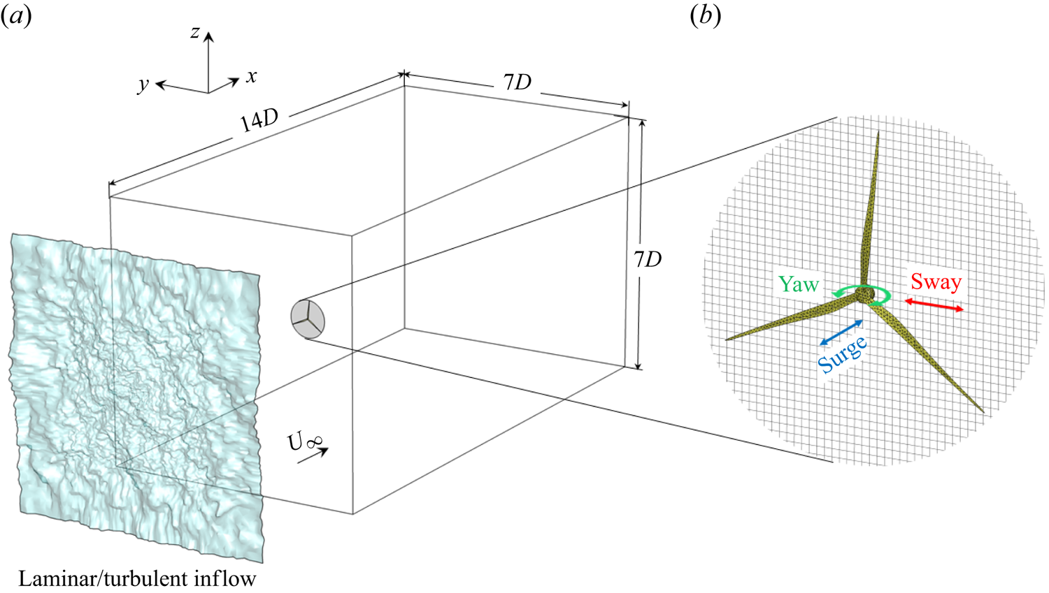
Due to the dynamic and complex environmental conditions in which they operate, the floating wind turbines exhibit motions with six degrees of freedom (Lyu, Zhang & Li Reference Lyu, Zhang and Li2019). In this study we focus on three representative motions, namely the sway (in-plane translation, along the  $y$ axis), the surge (out-of-plane translation, along the
 $x$ axis) and the yaw (out-of-plane rotation, along the
 $z$ axis) as illustrated in figure 2. When assuming an inflow without shear and an axisymmetric wake, yaw can be considered equivalent to pitch; sway can be considered equivalent to heave, following a coordinate transformation. At small amplitude, the roll motion of FOWT can be approximated by the sway motion since the centre of gravity is far below the rotor hub centre (Ribeiro, Casalino & Ferreira Reference Ribeiro, Casalino and Ferreira2023a). Here, we assume that the FOWT is forced to oscillate harmonically for each motion.
Schematics of the computational domain (a); the surface mesh of the actuator surface model and the Cartesian grid for the flow solver, with the three types of motion considered (b).
For the surge motion, the rotor translates in the streamwise direction  $(x)$, with a displacement of
 \begin{equation} \delta x_{h}(t) = A \sin{\left(\omega t \right)}. \end{equation}
For the sway motion, the rotor translates in the spanwise direction  $(y)$, with a displacement of
 \begin{equation} \delta y_{h}(t) = A \sin{\left(\omega t \right)}. \end{equation}
For the yaw motion, the rotor rotates around the vertical axis  $(z)$, with an angular displacement of
 \begin{equation} \delta \gamma_{h} (t) = A/R \sin{\left(\omega t \right)}. \end{equation}
The angle  $\gamma _{h}$ is equal to zero when the rotor is perpendicular to the streamwise direction.
The above definitions control the motions with  $A$ the linear displacement of the rotor tip and
 $\omega$ the motion's angular frequency. For a FOWT, the platform motion can be excited due to a combined load from turbulent wind and waves and the motion response falls in a large frequency range depending on the environment and the platform's natural frequency (Jonkman & Musial Reference Jonkman and Musial2010; Robertson et al. Reference Robertson2014). Previous studies (Li et al. Reference Li, Dong and Yang2022; Messmer et al. Reference Messmer, Hölling and Peinke2023) have estimated the Strouhal number generally falls in the range of
 $St \in [0.1, 1.5]$ for utility-scale wind turbines. The motion amplitude
 $A$ has been found to be in the order of
 $1\,\%D$ by a recent field measurement on a spar-type floater (Angelou et al. Reference Angelou, Mann and Dubreuil-Boisclair2023), which is known for small motion; larger motion amplitudes are found for semi-submersible floaters (Schliffke, Conan & Aubrun Reference Schliffke, Conan and Aubrun2023). As a detailed investigation on how the amplitude and the frequency affect the wake response has been presented for sway motion in our previous work (Li et al. Reference Li, Dong and Yang2022), the present study employs only representative values to showcase the wake response due to different motion types and to validate the predictive capacity of the proposed M2W model. These specific values will be presented later in the relevant context. An extra case without rotor motion is also included as the baseline.
Both laminar and turbulent inflows are considered. For all the cases, the simulation employs a rectangular computational domain as shown in figure 2. The length in the streamwise direction ( $x$) is
 $14D$ and is
 $7D$ in both the transversal (
 $y$) and the vertical (
 $z$) directions. The wind turbine is placed on the domain centreline, and the rotor axis is aligned with the
 $x$ direction. The distance from the inlet to the turbine is
 $3.5D$. The origin of the coordinate system coincides with the rotor hub centre.
The computational domain is discretized by the Cartesian grid. The grid has a uniform spacing in the  $y$ and
 $z$ directions of
 $\Delta y = \Delta z = D/40$ in the region
 $-2D< y<2D$ and
 $-2D< z<2D$ and is gradually stretched out of this region. The grid spacing in the streamwise direction is
 $\Delta x = D/20$. The rotor blade is discretized with an unstructured triangular mesh (see figure 2). Previous work has demonstrated that such a spatial resolution is sufficient to obtain mesh-independent results for both first- and second-order turbulence statistics in the far wake (Li & Yang Reference Li and Yang2021).
We impose the inflow velocity at the inlet boundary ( $x = -3.5D$). We neglect the wind shear and set a uniform wind speed of
 $U_\infty = 10\,{\rm m}\,{\rm s}^{-1}$ in the streamwise direction for the cases with laminar inflow. The periodic boundary condition is imposed in the lateral directions. The Neumann condition for the velocity (
 $\partial \boldsymbol {u}/\partial x = \boldsymbol {0}$) is imposed at the outlet (
 $x=10.5D$).
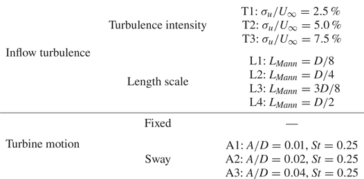
The wake response to different floating wind turbine motions is first investigated under uniform inflow conditions. The parameter space is summarized by table 1. All three motion types (surge, sway, yaw) are considered. The wind turbine motion amplitude is kept small. Our previous study has shown that the wind turbine wake is very sensitive to the rotor's side-to-side motion and that even small amplitude motion ( $A=0.01D$) can lead to large meandering amplitude in the far wake, especially for cases with uniform inflow (Li et al. Reference Li, Dong and Yang2022). Provided the present M2W model is based on the linear assumption, we set the motion amplitude to
 $A=0.01D$ in LES to keep the nonlinearity at a minimal level to facilitate the comparison between the model and the LES. To treat this small motion in LES, the aerodynamic force of the blade is first computed on the Lagrangian nodes of the actuator surface and is then distributed to the Eularian grid for the flow solver, employing the discretized smoothed delta function as the kernel (Yang et al. Reference Yang, Zhang, Li and He2009). It considers the distance between the Lagrangian and the Eularian nodes, so the motion of the rotor can be reflected even when the displacement is smaller than the grid size. The results of our previous LES study that employed the same numerical approach (Li et al. Reference Li, Dong and Yang2022) have been confirmed by Messmer et al. (Reference Messmer, Hölling and Peinke2023) using a wind tunnel experiment. Among the frequencies selected,
 $St \in \{ 0.1, 0.25, 0.5 \}$, our previous study (Li et al. Reference Li, Dong and Yang2022) has shown that
 $St = 0.25$ is close to the most sensitive forcing frequencies for the sway motion, while sway motions at
 $St=0.10$ and
 $St=0.50$ lead to less amplified wake meandering for the 5 MW reference wind turbine of the National Renewable Energy Laboratory. We will verify if the same sensitive frequency range is valid for all three motion types.
Parameter space for investigating the wake response to typical floating wind turbine motions under uniform inflow conditions.

To consider the effect of turbulence, we impose synthetic turbulence generated by the spectral tensor method of Mann (Reference Mann1994) at the inlet boundary of the computational domain, in addition to the uniform streamwise flow of  $U_\infty = 10\,{\rm m}\,{\rm s}^{-1}$. The control parameters of the synthetic turbulence are (i)
 $\alpha \epsilon ^{2/3}$ a scalar to control the TIs; (ii)
 $\varGamma$, a non-dimensional number for defining the anisotropy, setting to 3.9 according to the wind energy standard (IEC 2019); (iii)
 $L_{Mann}$, a length scale proportional to the size of the most energetic eddy, varies in
 $L_{Mann} \in \{D/8, D/4, 3D/8, D/2\}$, which are referred to as L1 to L4 in an increasing order. Taking
 $D=198$ m into account,
 $L_{Mann}$ falls into the range of 24.75 m to 99 m, containing the recommended value,
 $L_{Mann} = 33.6$ m for
 $z_{hub} \ge 60$ m, by IEC (2019). We generate a total of 12 turbulent inflows, with three TIs (shown in table 2) and four length scales. The obtained inflow turbulence length scales
 $L_{u_i}^{x_j}$ for different
 $L_{Mann}$ are shown in figure 3, which represents the spatial scales of turbulent eddies with the most energy for the three fluctuating wind velocity components
 $u_i = \{u_x, u_y, u_z\}$ in the streamwise (
 $x$), transverse (
 $y$) and vertical (
 $z$) directions, respectively (Nandi & Yeo Reference Nandi and Yeo2021). The integral lengths are computed with
 \begin{equation} L_{u_i}^{x_j} = \int_0^\infty \frac{\langle u_i(\boldsymbol{x})u_i(\boldsymbol{x}+\xi\boldsymbol{e_j})\rangle}{\left\langle u_i^2\right\rangle} \,\text{d} \xi. \end{equation}
Our previous study (Li et al. Reference Li, Dong and Yang2022) compared the wake of a fixed wind turbine and a sway wind turbine under inflow with different TIs but only a fixed  $L_{Mann}$ close to the L4 case, leaving the effect of inflow turbulence length scale unexplored. For this reason, the present work uses
 $L_{Mann}$ to control the inflow turbulence length scale, which has been found to be critical for the wake meandering of a fixed wind turbine (Espana et al. Reference Espana, Aubrun, Loyer and Devinant2011; Gambuzza & Ganapathisubramani Reference Gambuzza and Ganapathisubramani2023).
Componentwise TI of the synthetic turbulence imposed at the inlet for the turbulent inflow cases.

Integral length scale of velocity components  $u_i$ in directions
 $x_j$. Results are shown for the (a) streamwise, (b) transversal and (c) vertical directions.

For cases with turbulent inflow, we consider only the sway motion since it leads to the largest wake meandering (as shown in § 3) and has the potential to enhance the wake recovery (Li et al. Reference Li, Dong and Yang2022; Messmer et al. Reference Messmer, Hölling and Peinke2023). Three different sway amplitudes are investigated, i.e.  $A \in \{0.01D, 0.02D, 0.04D\}$, and are referred to as A1, A2 and A3, in increasing order. Increasing the motion amplitude is to strengthen the wake response, such that the motion-induced wake response can be distinguished from the background turbulence. The reduced frequency of the sway motion is equal to
 $St = 0.25$, falling near the most sensitive frequency for the wake's shear layer. The parameter space employed for investigating the joint effect of inflow turbulence and turbine motion is listed in table 3, containing 48 cases for LES.
Parameter space employed for investigating the joint effect of inflow turbulence and turbine motion on the wake evolution of a FOWT.
3. Wake response to rotor motions in uniform inflow
In this section we investigate the wake response to wind turbine motions by analysing the results of LES in uniform inflow condition.
3.1. Instantaneous wake
The wake behaviour for different rotor motions are first examined by comparing the instantaneous velocity deficit ( $\Delta u_x = u_x - U_\infty$) on the hub-height plane, as depicted in figure 4.
Instantaneous streamwise velocity deficit in the wake on the hub-height plane for a fixed rotor (a), a FOWT rotor with surge (b–d), sway (e–g) and yaw (h–j) motions. The frequency of rotor motion is  $St = 0.10, 0.25$, and
 $0.50$ for the first, second, and last column, respectively. All contours are plotted at the same time
 $tU_\infty /D = 60$. Inflow: uniform. Method: LES.

As seen, the wake of a fixed wind turbine remains nearly straight when travelling downstream due to the absence of incoming flow disturbances. Only small-scale fluctuations are observed in the far wake due to the wake-generated turbulence.
At  $St=0.1$, none of the three motions is able to generate remarkable changes to the wake, indicating the wake is nearly insensitive to the disturbances at this frequency regardless of the rotor motion types.
As the motion frequency increases to  $St=0.25$, the wake contour shows significant differences from the fixed turbine case. Firstly, the wake response is found to be dependent on the motion type. Specifically, the wake for cases with surge motion remains almost straight, but an alternating wind speed is found in the wake, where the wake is separated by regions with relatively higher and lower wind speeds. This accordion-like wake movement (Ramos-García et al. Reference Ramos-García, González Horcas, Pegalajar-Jurado, Kontos and Bredmose2022) is referred to as wake pulsing by Messmer et al. (Reference Messmer, Hölling and Peinke2023). In contrast, both sway and yaw motions induce obvious lateral wake motions, i.e. wake meandering, starting from
 $x\approx 5D$. Notably, the wake meandering caused by sway and yaw exhibits strong similarity, i.e. both have a wavy form with almost identical wavelengths, and both amplitudes gradually increase with downstream distance.
In figure 5 we compare the wake meandering caused by sway (a) and yaw (b) for cases with  $St = 0.25$. The wake trajectory is outlined by the centreline
 $y_c(x,t)$, computed as the weight centre of the velocity deficit as
 \begin{equation} y_c(x,t) = \frac{\int_{-\infty}^{+\infty} \Delta u_x(x,y,t) y\, \text{d}y}{\int_{-\infty}^{+\infty} \Delta u_x(x,y,t) \,\text{d}y }. \end{equation}
At this instant, it is found that the lateral motion of the wake trajectory  $y_c(x)$ is opposite in direction for sway (a) and yaw (b), when the motions are defined with (2.10) and (2.11) with
 $A=0.01D$ and
 $St=0.25$. This opposite wake motion is confirmed by computing the correlation coefficient of the instantaneous wake centre position time history at
 $x=8D$, which yields
 $\rho = -0.93$. Such an opposite wake centre displacement indicates that if the sway and the yaw motions are combined with different phase lags, the wake meandering can be either strengthened or weakened. To this end, a quick proof of concept is illustrated in figure 5, for cases with in-phase (c) and opposite-phase sway–yaw combinations (d). Here, in-phase refers to a direct combination of sway and yaw motions defined by (2.10) and (2.11), whereas the opposite-phase case employs a yaw motion with a
 $180^\circ$ phase lag. As seen, the wake meandering is significantly mitigated in figure 5(c) but enhanced in figure 5(d). The standard deviations of the instantaneous wake position
 $y_c(x=8D,t)$ are
 $0.24D$ (sway only),
 $0.20D$ (yaw only),
 $0.11D$ (sway yaw motion in-phase),
 $0.31D$ (sway yaw motion opposite-phase). However, such an interesting phase relation between sway and yaw can be neither explained straightforwardly using the rotor displacement nor with the LSA (Li et al. Reference Li, Dong and Yang2022) since an end-to-end M2W relation is not established in LSA. Such a phase-resolved prediction capability will be fulfilled by the model proposed by this work, as shown in § 4.3.
Instantaneous wake for cases with sway (a) and yaw (b). The mitigating case (c): the sway and the yaw motions are combined directly. The enhancement case (d): the yaw motion is lagged by half a period. The red dash-dot lines plot the wake centreline  $y_c(x)$ and the dashed lines approximate the wake boundary using
 $y_c(x)\pm 0.5D$. Inflow: uniform. Method: LES.

When further increasing the motion frequency to  $St=0.50$, figure 4 shows that the wake response becomes weaker for all motion types. The wake pulsing is still observed for the case with surge but its wavelength is reduced. For the cases with sway and yaw motions, the meandering of the wake is less apparent, while more velocity fluctuations at smaller scales are found compared with the wake of a fixed wind turbine.
3.2. Time-averaged wake
To investigate the wake recovery enhancement due to rotor motion, we compare the time-averaged velocity deficit  $\Delta \bar {u}_x = \bar {u}_x - U_\infty$ on the hub-height plane, as depicted in figure 6. Consistent with the findings for instantaneous wakes, the fastest wake recoveries are observed for the cases with sway and yaw motions at
 $St=0.25$. In these cases, the expansion rate of the time-averaged wake is significantly increased from
 $x \approx 5D$, where the onset of meandering is observed in the instantaneous wake, as shown by the counterparts of figure 4. Furthermore, the velocity profiles deviate noticeably from the Gaussian shape, which is caused by the non-Gaussian distribution of the instantaneous wake centre locations when motion-induced wake meandering amplitude is significant (Li et al. Reference Li, Dong and Yang2022). However, for the sway and the yaw motions at other frequencies, and for the surge motion at all three frequencies, the time-averaged wake closely resembles that of a fixed wind turbine. This observation is consistent with the wind tunnel measurements of Schliffke et al. (Reference Schliffke, Aubrun and Conan2020), which found that surge motion has only a weak effect on the time-averaged wake recovery.
Time-averaged velocity wake deficit contour on the hub-height plane and profiles at  $x = 2D, 4D, 6D, 8D$. See figure 4 for a detailed caption. Inflow: uniform. Method: LES.

Moreover, the wake recovery enhancement due to wind turbine motion is compared quantitatively in figure 7, by plotting the space–time-averaged velocity deficit  $\Delta \tilde {U}_x$. This space–time-averaged velocity deficit is obtained by averaging the time-averaged velocity deficit
 $\Delta \bar {u}_x$ over the wake region,
 $y \in [-0.5D, 0.5D]$, on the hub-height plane. As seen, at
 $St=0.1$, the curves for cases with different types of motion collapse, indicating that the effect of motion is negligible at this frequency for all motion types. However, at
 $St=0.25$, the velocity deficit is recovered by approximately
 $0.2U_\infty$ more at
 $x=10D$ for both sway and yaw motions compared with the fixed wind turbine case. In contrast, the effect of surge motion is still minimal. As the motion frequency increases to
 $St=0.5$, the wake recovery rate for sway and yaw motions is reduced, while that for the surge motion is slightly enhanced. At
 $x=10D$, the motion-enhanced extra wake recovery is 3.8 %, 8.3 % and 6.3 % of the free-stream wind speed
 $U_\infty$ for the surge, the sway and the yaw motions, respectively. It is worth noting the above comparison showcases the effect of the wake instability triggered by rotor motion and is based on a small rotor motion amplitude
 $A=0.01D$. Motions with large amplitudes that directly modify the wake, without triggering flow instability, are not considered in this study.
Space–time-averaged velocity deficit in the wake on the hub-height plane over  $-0.5D< y<0.5D$. Results are shown for motions at a reduced frequency of
 $St=0.10$ (a),
 $St=0.25$ (b) and
 $St=0.50$ (c). Inflow: uniform. Method: LES.

4. Resolvent-based M2W model
In the following we present a linear model for predicting the wake response to dynamic rotor motion. The structure of the M2W model is depicted in figure 1. The model's input is the time-averaged wake of a fixed wind turbine, which can be obtained conveniently from simulation (Li et al. Reference Li, Dong and Yang2022) or experiments (Iungo et al. Reference Iungo, Viola, Camarri, Porté-Agel and Gallaire2013). Based on the time-averaged wake, the first building block of the M2W model, i.e. the F2W model, is established using the resolvent of the LNSE (Towne, Schmidt & Colonius Reference Towne, Schmidt and Colonius2018; Jovanović Reference Jovanović2021), which will be introduced in § 4.1. The second building block is the M2F model, which parameterizes the effect of rotor motion as unsteady forces on a fixed actuator disk. This building block will be derived in § 4.2. Finally, the M2W prediction is achieved by connecting the two building blocks. The predictive capability of the M2W model will be verified against LES in § 4.3.
4.1. Forcing-to-wake model
The resolvent analysis is a powerful tool for predicting the response of a linear fluid system to forcing (Trefethen et al. Reference Trefethen, Trefethen, Reddy and Driscoll1993), either from external sources (Jovanović & Bamieh Reference Jovanović and Bamieh2005; Sipp et al. Reference Sipp, Marquet, Meliga and Barbagallo2010) or from the nonlinear term of the Navier–Stokes equations (McKeon & Sharma Reference McKeon and Sharma2010; Wu & He Reference Wu and He2023). To derive the resolvent-based F2W model, we apply the Reynolds decomposition to the variables of the Navier–Stokes equation as
 \begin{gather} \boldsymbol{u} = \bar{\boldsymbol{u}} + \delta \boldsymbol{u}, \end{gather}
 \begin{gather}p = \bar{p} + \delta p, \end{gather}
 \begin{gather}\boldsymbol{f} = \bar{\boldsymbol{f}} + \delta \boldsymbol{f}, \end{gather}
where  $\boldsymbol {u}$,
 $p$,
 $f$ represent the velocity, pressure and rotor forcing, respectively. The time-averaged part is denoted by the
 $\bar {{\cdot }}$ symbol and the perturbation part is denoted by the
 $\delta$ symbol. The time-averaged wake of a fixed wind turbine, obtained with LES, is employed as the time-averaged part.
The first assumption of the present model is the linear assumption, following which the evolution of small coherent perturbations due to rotor forcing can be described by the LNSEs as
 \begin{gather} \frac{\partial (\delta \boldsymbol{u})}{\partial t}+ (\boldsymbol{\bar{u}} \boldsymbol{\cdot} \boldsymbol{\nabla}) (\delta \boldsymbol{u}) + (\delta \boldsymbol{u} \boldsymbol{\cdot} \boldsymbol{\nabla}) \boldsymbol{\bar{u}} + \boldsymbol{\nabla} (\delta p) - \nu_{eff} \nabla^2 (\delta \boldsymbol{u}) = \mathcal{B} (\delta \boldsymbol{f}), \end{gather}
 \begin{gather}\boldsymbol{\nabla} \boldsymbol{\cdot} (\delta \boldsymbol{u}) = 0, \end{gather}
where the matrix  $\mathcal {B}$ defines the spatial restriction such that forcing
 $\delta \boldsymbol {f}$ is confined in the rotor region. The effect of the turbulent Reynolds stresses is approximated by
 $\nu _{eff} \nabla ^2 (\delta \boldsymbol {u})$ (Morra et al. Reference Morra, Semeraro, Henningson and Cossu2019), using an effective viscosity
 $\nu _{eff}$ (Del Alamo & Jimenez Reference Del Alamo and Jimenez2006; Symon et al. Reference Symon, Madhusudanan, Illingworth and Marusic2023).
Secondly, to ensure computational efficiency, the model assumes the axisymmetry of the wake and is derived in the cylindrical coordinate system. The state variables of the flow are expressed in the cylindrical coordinate system as
 \begin{equation} \boldsymbol{q}(x,r,\theta,t) = [p, \boldsymbol{u}]^{\rm T}= [p, u_x, u_r, u_\theta]^{\rm T}(x,r,\theta,t), \end{equation}
with  $u_x, u_r, u_\theta$ the velocity components in the axial
 $(x)$, radial
 $(r)$ and azimuthal
 $(\theta )$ directions, and
 $p$ the pressure. Similarly, the volume forcing to the flow is expressed as
 \begin{equation} \boldsymbol{f}(x,r,\theta,t) = [f_x, f_r, f_\theta]^{\rm T}(x,r,\theta,t). \end{equation}
With these notations, (4.4) and (4.5) can be formulated into a linear system of the fluctuation part  $\delta \boldsymbol {q}(x,r,\theta,t)$ as
 \begin{equation} \frac{\partial\delta \boldsymbol{q} }{\partial t}=\mathcal{L} \delta \boldsymbol{q} + \mathcal{B} \delta \boldsymbol{f}, \end{equation}
where the concrete form of  $\mathcal {L}$ is provided in Appendix A, following the standard procedure for linearizing the Navier–Stokes equations (Kaplan et al. Reference Kaplan, Jordan, Cavalieri and Brès2021).
Thirdly, we employ the effective viscosity (Symon et al. Reference Symon, Madhusudanan, Illingworth and Marusic2023) to model the effects of small-scale turbulence on the large turbulent coherent structures (Del Alamo & Jimenez Reference Del Alamo and Jimenez2006) in the wake, due to the large Reynolds number of the wind turbine wake. Looking for the optimal effective viscosity for resolvent analysis is still an ongoing topic in turbulence research (Gupta et al. Reference Gupta, Madhusudanan, Wan, Illingworth and Juniper2021; Pickering et al. Reference Pickering, Rigas, Schmidt, Sipp and Colonius2021). In this work, we employ a basic mean flow consistent effective viscosity. The effective viscosity is approximated by a linear fitting of the Reynolds shear stress  $\overline {u'_x u'_r}$ and the streamwise velocity gradient (
 $\mathrm {d} \bar {u}_x / \mathrm {d} r$) from LES of a fixed wind turbine wake as
 \begin{equation} \nu_{eff} ={-}\frac{\overline{u'_x u'_r}}{\mathrm{d} \bar{u}_x / \mathrm{d} r}. \end{equation}
In the present model, the effective viscosity is assumed to be dependent only on the streamwise location  $(x)$, i.e.
 $\nu _{eff} = \nu _{eff}(x)$ is computed at each downstream location to account for its streamwise variation.
Due to the linear nature of the model, the solution is sought in the frequency domain. To this end, the state variables and the forcing are decomposed using the Fourier series, by assuming the homogeneity in time and in the azimuthal direction as
 \begin{gather} \delta \boldsymbol{f}(x, r, \theta, t) = \sum_{\omega ={-}\infty}^{\infty} \sum_{m={-}\infty}^{\infty} \hat{\boldsymbol{f}}_{m,\omega}(x, r) \exp \left(\mathrm{i}(m \theta-\omega t)\right), \end{gather}
 \begin{gather}\delta \boldsymbol{q}(x, r, \theta, t) = \sum_{\omega ={-}\infty}^{\infty} \sum_{m={-}\infty}^{\infty} \hat{\boldsymbol{q}}_{m,\omega}(x, r) \exp \left(\mathrm{i}(m \theta-\omega t)\right) , \end{gather}
with  $\mathrm {i} = \sqrt {-1}$ the imaginary unit,
 $m$ the azimuthal wavenumber and
 $\omega$ the angular frequency. Substituting this ansatz to the linearized equation (4.8) results in an input–output system for each
 $(m,\omega )$ pair as
 \begin{equation} (-\mathrm{i} \omega \mathcal{I}-\mathcal{L}_{m})\hat{\boldsymbol{q}}_{m,\omega}(x,r) = \mathcal{B} \hat{\boldsymbol{f}}_{m,\omega}(x,r), \end{equation}
or equivalently,
 \begin{equation} \hat{\boldsymbol{q}}_{m,\omega}(x,r) = \mathcal{R}_{m,\omega} \,\hat{\boldsymbol{f}}_{m,\omega}(x,r), \end{equation}
with  $\mathcal {R}_{m,\omega } = (-\mathrm {i} \omega \mathcal {I}-\mathcal {L}_{m})^{-1}\mathcal {B}$ the resolvent operator that transfers the forcing mode
 $\hat {\boldsymbol {f}}_{m,\omega }(x,r)$ to the response mode
 $\hat {\boldsymbol {q}}_{m,\omega }(x,r)$. Here
 $\mathcal {I}$ is the identity matrix and
 $\mathcal {L}_{m}$ is provided in Appendix A.
The above equation is discretized in a two-dimensional domain of  $-2D< x<10D$ and
 $0< r<3.5D$. The grid spacing and the discretization scheme in the streamwise direction are the same as LES with a number of grid points
 $N_x = 240$. In the radial direction, Chebyshev polynomials are employed to discretize the equation with
 $N_r = 100$ collocation points. The same mapping technique employed by Li et al. (Reference Li, Dong and Yang2022) is adopted to set half of the points inside the wake region
 $0< r<0.5D$.
4.1.1. Optimal rotor forcing and wake response
As the resolvent operator  $\mathcal {R}_{m,\omega }$ connects the rotor forcing to the wake response, the optimal rotor forcing leading to the strongest wake response can be found by analysing this linear operator. To this end, we define the energy gain of the resolvent operator as
 \begin{equation} G_{opt}^2\left(\omega, m\right)=\max _{\hat{\boldsymbol{f}}_{\omega,m}} \frac{\|\hat{\boldsymbol{q}}_{\omega,m}\|_E^2}{\|\,\hat{\boldsymbol{f}}_{\omega,m}\|_f^2}, \end{equation}
which denotes the energy amplification in the wake to the rotor forcing. The energy norm of the wake response and of the rotor forcing is defined as
 \begin{gather} \|\hat{\boldsymbol{q}}\|_E^2 = \hat{\boldsymbol{q}}^H \boldsymbol{W}_q \hat{\boldsymbol{q}} = \int_\varOmega \big( \hat{u}^2_x + \hat{u}^2_r + \hat{u}^2_\theta \big) r \,\text{d}\theta \,\text{d}r \,\text{d}\kern0.06em x, \end{gather}
 \begin{gather}\|\,\hat{\boldsymbol{f}}\|_f^2 = \hat{\boldsymbol{f}}^H \boldsymbol{W}_f \hat{\boldsymbol{f}} = \int_\varGamma \big( \hat{f}^2_x + \hat{f}^2_r + \hat{f}^2_\theta \big) r \,\text{d}\theta\, \text{d}r, \end{gather}
where  $\boldsymbol {W}_q$ and
 $\boldsymbol {W}_f$ are the weight matrices of the discretized energy norm. The integration domains for the energy norm definition expand
 $0< x<10D$,
 $0< r<3.5D$,
 $0<\theta <2{\rm \pi}$ for
 $\varOmega$ and
 $x=0$,
 $0< r<3.5D$,
 $0<\theta <2{\rm \pi}$ for
 $\varGamma$.
The optimization problem defined in (4.14) is equivalent to finding the largest eigenvalue of the following problem (Garnaud et al. Reference Garnaud, Lesshafft, Schmid and Huerre2013):
 \begin{equation} \boldsymbol{W}_f^{{-}1} \boldsymbol{R}^H \boldsymbol{W}_q \boldsymbol{R} \hat{\boldsymbol{f}} = \lambda \hat{\boldsymbol{f}}. \end{equation}
Here the largest eigenvalue is equal to the square of the optimal gain ( $\lambda _{max} = G^2_{opt}$), and the eigenvector corresponds to the optimal rotor forcing mode (
 $\hat {\boldsymbol {f}}_{opt}$). The optimal response mode is obtained by solving (4.13) once the optimal forcing mode is obtained.
One issue related to the computational cost is that the explicit construction of the bi-global resolvent operator  $\mathcal {R}_{m,\omega } = (-\mathrm {i} \omega \mathcal {I}-\mathcal {L}_{m})^{-1}\mathcal {B}$ gives rise to a prohibitive memory cost due to the storage of a large dense matrix of
 $(4\times N_x \times N_r) \times (4\times N_x \times N_r)$. This problem is circumvented by employing the Arnoldi algorithm, as described by Martini et al. (Reference Martini, Rodríguez, Towne and Cavalieri2021) and Kaplan et al. (Reference Kaplan, Jordan, Cavalieri and Brès2021).
Figure 8 depicts the computed optimal gain  $G_{opt}(St, m)$ as a function of the forcing frequency
 $St$ and the azimuthal wavenumber
 $m$. The curve of the optimal gain for the rotor forcing with
 $m = 0$ is found to have a flat plateau in
 $0.2< St<0.4$ where the gain is elevated. For
 $m \neq 0$, the optimal gains of the opposite azimuthal wavenumbers show a similar variation via
 $St$, but differ slightly as a result of the non-zero time-averaged rotational velocity of the wake. For the gains of the rotor forcing with
 $m = \pm 1$, they both have a distinct peak near
 $St \approx 0.25$, which is the largest among all azimuthal wavenumbers considered. Further increasing the wavenumber beyond
 $|m| \ge 2$ reduces the magnitude of the optimal gain. From an application aspect view, the rotor forcings with azimuthal wavenumbers
 $m=0$ and
 $m=\pm 1$ are important because they can be induced by floating wind turbine motions, as will be shown in § 4.2. Bottom fixed turbines can also generate these rotor forcings with wake control techniques such as the dynamic induction control (DIC, Goit & Meyers Reference Goit and Meyers2015)
 $(m=0)$ and the helix wake control approach
 $(m=\pm 1)$ (Frederik et al. Reference Frederik, Doekemeijer, Mulders and van Wingerden2020). We note that the most unstable modes have an azimuthal wavenumber of
 $m = \pm 1$, which agrees with the result obtained by Viola et al. (Reference Viola, Iungo, Camarri, Porté-Agel and Gallaire2014) using local LSA with eddy viscosity.
Optimal gain as a function of the forcing frequency  $St$. Each branch represents a different azimuthal wavenumber
 $m$. Inflow: uniform. Method: F2W model.

It is also worth noting that the optimal gain is dependent on the definition of the energy norm of the wake response and rotor forcing. One may change the definition of (4.15) to focus on other wake properties. One example of using the energy of streamwise velocity fluctuation to define the energy gain is shown in Appendix B.1.
Furthermore, Appendix B.2 investigates the sensitivity of the optimal gain to the effective viscosity ( $\nu _{eff}$), because the present model employs a simple
 $\nu _{eff}$ modelling that does not account for the possible variation of
 $\nu _{eff}$ due to the dynamic wake response. The results show that, even
 $\nu _{eff}$ is augmented or diminished by a factor of two, the present model is able to predict the peak frequency leading to the maximum gain reasonably well for cases with
 $m=1$, which leads to the strongest wake response, where the peak frequency predicted by the model consistently falls in the range
 $0.2 < St < 0.3$. However, it is noteworthy that the magnitude of the optimal gain demonstrates sensitivity to
 $\nu _{eff}$. An increase in effective viscosity tends to stabilize the flow, thereby diminishing the magnitude of the optimal gain. As the result suggested, the present model can be employed to effectively narrow the focus of the frequency range for flow control purposes, such that a more detailed investigation could be realized through methods like model experiments or LES, where the nonlinear effects leading to the uncertainty of
 $\nu _{eff}$ can be incorporated properly. Moreover, advanced effective viscosity modelling can also be developed to enhance the predictive capability of the proposed model.
The spatial modes of the optimal rotor forcing are plotted in figure 9 for the case with  $St=0.25$. The streamwise forcing is larger than the radial and azimuthal forcing components, indicating that the wake is more sensitive to forcing in the streamwise direction. The streamwise and radial components of the forcing modes for
 $m=\pm 1$ are similar, except the rotational directions which are the opposite. Larger discrepancies are observed in the azimuthal component, due to the non-zero time-averaged rotational velocity of the wake.
The real part of the spatial mode of the optimal rotor forcing predicted by the resolvent analysis at  $St = 0.25$ for the azimuthal wavenumber
 $m=0$ (a–c),
 $m=1$ (d–f),
 $m=-1$ (g–i). The forcing modes are normalized such that
 $\|\hat {\boldsymbol {f}}\|_{f} = 1$, as defined by (4.16). Inflow: uniform. Method: F2W model.

The optimal forcing is also dependent on the forcing frequency as depicted by figure 10, where the forcing modes for  $St=0.10$, 0.25 and 0.50 are compared for the same azimuthal wavenumber
 $m=1$. As seen, the spatial patterns are found to be similar for different motion frequencies. However, increasing the Strouhal number generally moves the forcing region toward the edge of the disk, and the forcing structure becomes narrower. A similar trend is also found for other azimuthal wavenumbers but is not shown for conciseness.
Same as figure 9 but for different  $St$ with the azimuthal wavenumber
 $m=1$.

The wake response under the optimal forcing is depicted in figure 11 for cases with  $m=0$ and
 $m = \pm 1$,
 $St = 0.10, 0.25, 0.50$. These modes are plotted in the
 $rOx$ plane where
 $r=0$ corresponds to the wake centreline. For all cases, the wake response shows a wavy pattern in the
 $x$ direction, as the fluctuating velocity field behaves as a wave travelling downstream. The wavelength of the coherent structures is found to be negatively related to the forcing Strouhal number
 $St$, as one can expect. Besides, the streamwise development of the fluctuation magnitude is also dependent on the Strouhal number. For cases with
 $St=0.10$ and
 $0.25$, the velocity fluctuation generally increases with downstream location, while increasing the frequency to
 $St=0.5$ dampens the far wake fluctuation for
 $x>5D$.
The real part of the optimal response of the wake velocity predicted by the resolvent analysis for the azimuthal wavenumbers  $m=0$ (a–c),
 $m=1$ (d–f) and
 $m=-1$ (g–i) with forcing frequencies of
 $St = 0.10, 0.25, 0.50$. The modes are plotted in a two-dimensional
 $rOx$ plane, where
 $\hat {u}_x$,
 $\hat {u}_r$ and
 $\hat {u}_\theta$ represent the velocity fluctuation in the streamwise, radial and azimuthal directions. The response modes are normalized such that
 $\|\hat {\boldsymbol {q}}\|_{E} = 1$, as defined by (4.15). Inflow: uniform. Method: F2W model.

The above method provides an efficient way to relate the wake response due to rotor forcing by the resolvent operator. To find the optimal forcing and response it takes approximately several minutes for each pair of wavenumber and frequency  $(m, St)$ on a desktop computer. However, since the rotor forcing is not directly related to the motion of FOWT, one cannot predict the wake response in a motion-specific manner yet. This shortcoming necessitates the development of a M2F model of the floating wind turbine in the next subsection.
4.2. Motion-to-forcing model
In this section we derive the second part of the M2W model, i.e. the M2F model. The idea of this modelling is to replace wind turbine motion with equivalent force. The model proposed here is an actuator disk fixed at the time-averaged position of the moving wind turbine, but exerting unsteady motion-dependent forces. To remain consistent with the resolvent F2W model, we decomposed the force on the actuator disk  $\boldsymbol {f}(r,\theta,t)$ into a time-averaged thrust and an unsteady part as follows:
 \begin{equation} \boldsymbol{f}(r,\theta,t) = [-\bar{f}_T(r)+\delta f_x(r,\theta,t), \delta f_r(r,\theta,t), \bar{f}_\theta(r)+ \delta f_\theta(r,\theta,t)]^{\rm T}. \end{equation}
The time-averaged force on the rotor is simplified as a normal thrust  $\bar {f}_T(r)$ and rotational force
 $\bar {f}_\theta (r)$. The radial variation of the thrust force is maintained to account for the blade design, which has been shown to be important for the wake recovery (Dong et al. Reference Dong, Qin, Li and Yang2023). Here
 $\bar {f}_T(r)$ is computed from the time-averaged blade thrust
 $\bar {F}_T(r)$ as
 \begin{equation} \bar{f}_T(r) = \frac{m\ {\cdot}\ \bar{F}_T(r) \delta r}{ 2{\rm \pi} r \delta r} = \frac{m\ {\cdot}\ \bar{F}_T(r) }{2 {\rm \pi}r }, \end{equation}
where  $m=3$ is the number of blades and
 $\delta r \rightarrow 0$ is the width of an annulus at
 $r$. Furthermore, the thrust coefficient
 $\bar {C}_T(r)$ of the actuator disk is computed as
 \begin{equation} \bar{C}_T(r) = \frac{\bar{f}_T(r)}{\dfrac{1}{2} U_\infty^2}. \end{equation}
Figure 12 shows the time-averaged blade forces (a) and force coefficients of the rotor disk (b) obtained from the LES for different turbine motions. As seen,  $\bar {F}_T(r)$ and
 $\bar {C}_T(r)$ are almost unaffected by the rotor motion, because the oscillatory motion is relatively small, which is consistent with the experiments with model wind turbine rotors (Fontanella et al. Reference Fontanella, Zasso and Belloli2022; Meng et al. Reference Meng, Su, Guo, Qu and Lei2022a). From the theoretical aspect, recent studies of Wei & Dabiri (Reference Wei and Dabiri2023) and Heck, Johlas & Howland (Reference Heck, Johlas and Howland2023) have established relations between the thrust force for wind turbines with surge motion velocity amplitudes and yaw angles. For example, Wei & Dabiri (Reference Wei and Dabiri2023) has shown that the time-averaged rotor thrust of a periodically surging wind turbine (
 $\bar {F}_T$) is related to that of a stationary wind turbine
 $\bar {F}_{T,0}$ as follows:
 \begin{equation} \frac{\bar{F}_T}{\bar{F}_{T,0}} = 1 + \frac{1}{2}\frac{{u}^2_h}{U^2_\infty}. \end{equation}
Here  $u_h = A\omega$ is the motion amplitude of the rotor. The above equation indicates that the motion-induced thrust variation is small (
 ${u}_h \approx 0.016U_\infty$,
 ${u}^2_h \approx 0.0003 U^2_\infty$ for
 $A=0.01D$ and
 $St=0.25$;
 ${u}_h \approx 0.13 U_\infty$,
 ${u}^2_h \approx 0.017 U^2_\infty$ for
 $A=0.04D$ and
 $St=0.5$). For yaw motion, Heck et al. (Reference Heck, Johlas and Howland2023) also demonstrates a quadratic dependence of the thrust change with the yaw angle, which can also be ignored for
 $\gamma \ll 1$. For this reason, we assume that the thrust force and the thrust coefficient
 $\bar {C}_T(r)$ for all motions with small amplitudes can be approximated by those of a stationary wind turbine. The rotational force coefficient
 $\bar {C}_\theta (r)$ can also be computed by the same approach.
Comparison of time-averaged blade forces (a) and force coefficients of the rotor disk (b) for different motion types. The normal forces ( $\bar {F}_T$) and coefficients (
 $\bar {C}_T$) are plotted in colour and the rotational ones (
 $\bar {F}_\theta$ and
 $\bar {C}_\theta$) are plotted in grey. The reduced frequency of the motion is equal to
 $St = 0.25$ and the amplitude is
 $A=0.01D$. Inflow: uniform.

In the following we derive a linear M2F model to compute the unsteady force on the actuator disk induced by surge, sway and yaw motions, taking only the time-averaged force coefficients ( $\bar {C}_T(r)$ and
 $\bar {C}_\theta (r)$) as input and assuming that the motion amplitude is small.
4.2.1. Surge
The surge motion refers to the displacement in the streamwise direction ( $x$) as shown in figure 13(a). This motion generates a streamwise velocity of the rotor, denoted as (
 $u_{h}(t) = \delta \dot {x}_{h}(t)$), which alters the relative velocity between the free stream and wind turbine. To account for this variation, the thrust of the actuator disk is computed with a corrected wind speed
 $U_{rel} = U_\infty - \delta \dot {x}_{h}(t)$, while the thrust coefficient is assumed to equal
 $\bar {C}_T(r)$. This assumption is validated by examining the blade force results from LES with small
 $u_{h}(t)$. Based on these assumptions, the unsteady part of the rotor forcing is computed as
 \begin{align} \delta f_x(r,\theta,t) &
={-} \left( \tfrac{1}{2} U_{rel} ^2 \bar{C}_T(r) -
\tfrac{1}{2} U_\infty^2 \bar{C}_T(r) \right) \nonumber\\ & =
\tfrac{1}{2} \bar{C}_T(r) ( 2 U_\infty \delta \dot{x}_{h}(t)
- \delta \dot{x}^2_{h}(t))\nonumber\\ & \approx U_\infty
\bar{C}_T(r) \delta \dot{x}_{h}(t).
\end{align}
The minus sign at the first step reflects that the thrust force points in the opposite direction of  $x$ of the coordinate system. In the final step of (4.22), linear approximation is employed to truncate the high-order terms of
 $\delta \dot {x}_{h}(t)$, assuming
 $\delta \dot {x}_{h}(t) \ll U_\infty$. Substituting the harmonic surge displacement in (2.9)–(4.22) yields the unsteady streamwise forcing for harmonic surge motion as
 \begin{equation} \delta f_x(r,\theta,t) \approx \omega A \cos(\omega t) U_\infty \bar{C}_T(r) . \end{equation}
Similarly, the azimuthal component can be computed as
 \begin{equation} \delta f_\theta (r,\theta,t) \approx{-}\omega A \cos(\omega t) U_\infty \bar{C}_\theta(r) . \end{equation}
The resulting unsteady forcing is depicted in figure 14(a–c).
Schematics of floating wind turbine motion for surge (a), sway (b) and yaw (c). The red solid line outlines the instantaneous rotor position and the black dashed line shows the time-averaged rotor position. Red arrows illustrate the motion. The coordinates of  $O=(0,0,0)$ and
 $O'=(\delta x_{h}(t),\delta y_{h}(t),\delta z_{h}(t))$. The derived unsteady force is applied only inside the black dashed circle.

Spatial mode of the linearized unsteady forcing for surge motion (a–c), sway motion (d–f) and yaw motion (g–i). Plots (a,d,g), (b,e,h) and (c,f,i) show the streamwise, radial and azimuthal components of the rotor forcing, respectively. The forcing is computed for the cases with the reduced motion frequency  $St = 0.25$. All modes are normalized by
 $A U^2_\infty$. Method: M2F model.

4.2.2. Sway
The sway motion refers to the side-to-side translation of the rotor as shown in figure 13(b). Compared with surge motion, sway does not affect the axial relative velocity, indicating that the rotor thrust remains almost constant in the rotor-following frame of reference. However, since the thrust moves with the wind turbine, an unsteady variation of the thrust is generated in the ground-fixed frame of reference, which can be expressed as
 \begin{align} \delta f_x(r,\theta,t) & ={-}(f_T(r,\theta,t) - \bar{f}_T(r)) \nonumber\\ & ={-}\left(\frac{1}{2} U_\infty^2 \bar{C}_T(r'(t)) - \frac{1}{2} U_\infty^2 \bar{C}_T(r)\right)\nonumber\\ & \approx{-}\frac{1}{2} U_\infty^2 \frac{\partial \bar{C}_T(r)}{\partial r} (r'(t)-r)\nonumber\\ & \approx \frac{1}{2} U_\infty^2 \frac{\partial \bar{C}_T(r)}{\partial r} \cos{\theta} \delta y_{h}(t). \end{align}
Here,  $r$ and
 $r'(t)$ denote the distance from a point
 $P(0,y,z)$ to the time-averaged rotor centre
 $O = (0,0,0)$ and to the instantaneous wake centre
 $O'(t) = (0,\delta y_{h}(t),0)$, respectively, as illustrated in figure 13(b). The distance to the moving hub centre is computed as
 $r'(t) = \sqrt {(y- \delta y_{h}(t))^2 + z^2}$. Assuming small
 $\delta y_{h}(t)$, the last step in the equation is achieved by using the approximation
 \begin{align} r'(t) -r & = \sqrt{(y- \delta y_{h}(t))^2 + z^2} - \sqrt{y^2 + z^2} \nonumber\\ & \approx{-}\frac{y}{\sqrt{y^2 + z^2}}\delta y_h(t) \nonumber\\ & ={-} \cos {(\theta)} \delta y_{h}(t). \end{align}
Substituting  $\delta y_{h}(t)$ defined in (2.10) into (4.25) yields an unsteady streamwise forcing as
 \begin{equation} \delta f_x(r,\theta,t) \approx \frac{A}{2} \sin{(\omega t)} U_\infty^2 \frac{\partial \bar{C}_T(r)}{\partial r} \cos{\theta} . \end{equation}
Similarly, the unsteady forces in the azimuthal direction are modelled as
 \begin{equation} \delta f_\theta(r,\theta,t) \approx{-}\frac{A}{2} \sin{(\omega t)} U_\infty^2 \frac{\partial \bar{C}_\theta(r)}{ \partial r} \cos{\theta}. \end{equation}
Figure 14(d–f) illustrate the spatial mode of the unsteady forcing for the sway motion.
4.2.3. Yaw
The yaw motion corresponds to the rotational motion along the  $z$ axis, which induces a misalignment between the rotor-normal direction and the streamwise direction as shown in figure 13(c). The direction vector of the thrust depends on the yaw angle
 $\gamma _{h}(t)$ as follows:
 \begin{equation} \boldsymbol{n} = [-\cos{\gamma_{h}(t)}, - \sin{\gamma_{h}(t)},0]. \end{equation}
The leading-order effect of this directional variation is a side force in the transverse direction,
 \begin{align} \delta f_y(r,\theta,t) & ={-} \bar{f}_T(r) \sin{\left( \delta \gamma_{h}(t) \right)} \nonumber\\ & \approx{-}\tfrac{1}{2} U_\infty^2 \bar{C}_T(r) \delta \gamma_{h}(t), \end{align}
with Taylor expansion applied in the last step, assuming a small yaw angle  $|\delta \gamma _h(t)| \ll 1$. The lateral force
 $\delta f_y(r,\theta,t)$ is projected in the radial (
 $r$) and azimuthal (
 $\theta$) directions of the cylindrical coordinates, yielding
 \begin{align} \delta f_r(r,\theta,t) &= \delta f_y(r,\theta,t) \cos \theta \nonumber\\ & \approx{-}\tfrac{1}{2} U_\infty^2 \bar{C}_T(r) \delta \gamma_{h}(t) \cos \theta, \end{align}
 \begin{align} \delta f_\theta(r,\theta,t) &={-}\delta f_y(r,\theta,t) \sin \theta \nonumber\\ & \approx \tfrac{1}{2} U_\infty^2 \bar{C}_T(r) \delta \gamma_{h}(t) \sin \theta. \end{align}
Substituting the prescribed harmonic yaw motion defined in (2.11) into (4.31) and (4.32), the unsteady forcing caused by harmonic yaw motion is expressed as
 \begin{gather} \delta f_r(r,\theta,t) \approx{-}\frac{A}{2R}\sin{(\omega t)} U_\infty^2 \bar{C}_T(r) \cos \theta, \end{gather}
 \begin{gather}\delta f_\theta(r,\theta,t) \approx \frac{A}{2R}\sin{(\omega t)} U_\infty^2 \bar{C}_T(r) \sin \theta. \end{gather}
The unsteady forcing in the streamwise direction, mainly contributed by the time-averaged rotational force, is expressed as
 \begin{equation} \delta f_x(r,\theta,t) ={-} \frac{A}{2R} \sin(\omega t) U_\infty^2 \bar{C}_\theta(r) \sin\theta. \end{equation}
The spatial modes of the unsteady forcing are illustrated in figure 14(g–i).
4.2.4. Summary of M2F model
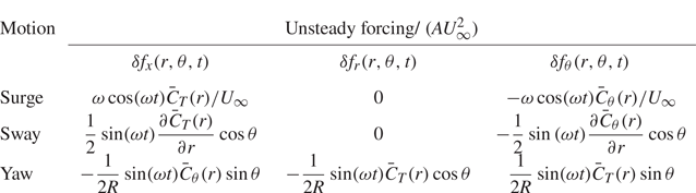
Table 4 summarizes the unsteady forcing for a FOWT undergoing harmonic surge, sway and yaw motions. Their spatial modes are plotted in figure 14. As seen, the forcing appears in different directions and has different azimuthal dependencies. The forcing for surge motion is axisymmetric, i.e. the azimuthal wavenumber is zero ( $m=0$). For sway and yaw motions, the forcing shows a side-to-side pattern, which can be decomposed into
 $m=\pm 1$ components. Moreover, we note that the magnitude of surge forcing is directly proportional to the motion frequency
 $\omega$. For sway and yaw motion, the motion frequency does not explicitly influence the forcing magnitude.
It is important to note that under the current uniform inflow condition, vertical and lateral motions (heave and sway) can be considered equivalent, differing only in their direction of motion. Similarly, the equivalence between pitch and yaw can be achieved through a change of coordinates. Roll motion around the turbine's centre of gravity results in a side-to-side motion at the rotor's height, which can be approximated as lateral motion (sway). Furthermore, the forcings of these elementary motions can be employed to compose forcings of complex, realistic motions.
4.3. Prediction of the M2W model for uniform inflow
In this subsection we show that the wake response of a FOWT can be predicted in an end-to-end manner by connecting the M2F and F2W models.
Firstly, the motion-induced forcing is projected to the basis functions  ${\rm e}^{\mathrm {i}(m\theta -\omega t)}$, as defined in (4.10), to obtain the corresponding forcing modes
 $\hat {\boldsymbol {f}}_{m, \omega }(x,r)$. Secondly, these forcing modes are then substituted into (4.13) of the F2W model to solve for the response modes
 $\hat {\boldsymbol {q}}_{m, \omega }(x,r)$. Finally, the wake response is reconstructed with (4.11). It is worth noting that the above procedure is not limited to the rotor forcings derived in § 4.2. The unsteady rotor forcing obtained by other computational methods can also be employed as input.
Taking the streamwise forcing induced by the sway motion as an example, it can be projected on four basis functions as
 \begin{equation} \delta f_x(r, \theta,
t) ={-}\frac{A U^2_\infty}{8\mathrm{i}}\frac{\partial
\bar{C}_T(r)}{\partial r} \left({\rm
e}^{\mathrm{i}(\theta-\omega t) } - {\rm
e}^{-\mathrm{i}(\theta-\omega t)} +{\rm
e}^{\mathrm{i}(-\theta-\omega t)} - {\rm
e}^{-\mathrm{i}(-\theta-\omega t)} \right).
\end{equation}
The coefficient of each basis function,  ${\rm e}^{\mathrm {i}(m \theta - n \omega t)}$, forms the spatial modes as follows:
 \begin{equation} \hat{f}^x_{ m, n \omega}(x=0,r) ={-} n \frac{A U^2_\infty}{8\mathrm{i}}\frac{\partial \bar{C}_T(r)}{\partial r} \end{equation}
with  $m = \pm 1$ and
 $n=\pm 1$. The forcing components in the radial and azimuthal directions can be decomposed similarly. By substituting all forcing modes into (4.13) and solving for the wake response mode-by-mode, the final wake response is
 $$\begin{gather} \delta \boldsymbol{q}(x, r,\theta, t) = \hat{\boldsymbol{q}}_{1, \omega}(x,r) {\rm e}^{\mathrm{i}(\theta-\omega t) } + \hat{\boldsymbol{q}}_{{-}1, -\omega}(x,r) {\rm e}^{-\mathrm{i}(\theta-\omega t) } \nonumber\\ + \,\hat{\boldsymbol{q}}_{{-}1, \omega}(x,r) {\rm e}^{\mathrm{i}(-\theta-\omega t) } +\hat{\boldsymbol{q}}_{1, -\omega}(x,r) {\rm e}^{-\mathrm{i}(-\theta-\omega t) }. \end{gather}$$
The wake response for FOWT subject to the surge or the yaw motions are computed with the same procedure.
Figure 15 depicts the three-dimensional coherent structure computed with the M2W model for the surge, sway and yaw motions. All the motions have the same frequency  $St = 0.25$ and the same amplitude
 $A=0.01D$. For surge motion, the velocity fluctuation is distributed uniformly in the azimuthal direction, while for sway and yaw motions, the streamwise velocity fluctuation mainly resides on the lateral sides of the wake. These spatial modes are consistent with the wake pulsing pattern for the surge motion and the wake meandering phenomenon for the sway and yaw motions.
Streamwise velocity fluctuation predicted by the M2W model for surge (a), sway (b) and yaw (c) at  $St=0.25$. The red and blue surfaces correspond to the isocontour of
 $|\delta u_x| = 0.05 U_\infty$, respectively. The base flow is depicted by a light blue shadow. Inflow: uniform. Method: M2W model.

The wake response is further analysed on the hub-height plane. Figure 16(a) displays the spatial modes of the velocity fluctuation ( $\hat {u}_x$ and
 $\hat {u}_y$) predicted by the M2W model at
 $St=0.25$, and is compared with the Fourier modes obtained with LES in figure 16(b). It is worth noting that all contours are plotted with the same magnitude allowing a direct comparison. As seen, the proposed M2W model predicts correctly the response modes compared with the LES in terms of flow structures. For surge motion, the pulsing mode of the wake observed in the instantaneous wake contour (figure 4) is revealed as a symmetric alternation of the streamwise velocity along the centreline. Furthermore, the lateral velocity is opposite in sign across the wake centreline, indicating a varicose deformation of the wake. For the sway and yaw motions that lead to wake meandering, the model predicts an anti-symmetric mode for streamwise velocity fluctuation, while the lateral velocity fluctuation spans throughout the entire wake. Moreover, the M2W model is capable of predicting the difference in the near wake for the sway and yaw motions. For the sway motion, an obvious anti-symmetric streamwise velocity fluctuation is found immediately behind the tip and the root of the blade, coincident with the rotor forcing distribution (see figure 14d). In comparison, the yaw motion induces a relatively smaller streamwise velocity fluctuation in the near wake, since the yaw motion does not result in a streamwise forcing near the rotor tip (see figure 14g–i). Thanks to the motion-specific modelling, the M2W model provides a phase-resolved prediction of the wake response that captures very well the phase opposition in the far wake for the sway and yaw motions. The predicted spatial modes are also comparable to the Fourier modes of the LES results. However, when comparing the model's prediction quantitatively with the LES, we notice some discrepancies in the far wake. The linear model systematically underestimates the wavelength of the velocity fluctuation, e.g. the coherent structures of the LES travel approximately one-quarter of a wavelength faster than those predicted by the M2W model at
 $x=10D$ for all motion types. This difference should be attributed to the base flow employed by the M2W model, i.e. the time-averaged wake of a fixed wind turbine. With such a base flow, the increase of wind speed in the far wake enhanced by turbine motions (in figure 7) is not accounted for. This underestimated wind speed in the base flow that might also explain the diamond pattern of
 $\hat {u}_x$ in the far wake for cases with sway and yaw, predicted by the M2W model, since the velocity near the wake centre is apparently slower than in the free stream for the base flow employed. In contrast, these structures are almost square in the result of LES, because these flow structures are convected by the actual wake velocity taking into account the enhanced wake recovery in LES.
Real part of the spatial mode of the fluctuating velocity on the hub-height plane, predicted by the M2W model (a) and the Fourier modes of LES (b). Here  $\hat {u}_x$ and
 $\hat {u}_y$ represent the modes of streamwise and lateral components, respectively. The motions have an amplitude of
 $A=0.01D$ and a reduced frequency of
 $St = 0.25$. Inflow: uniform.

The predictive capability of the M2W model is further verified at  $St=0.10$ and
 $St=0.50$ in figures 17 and 18. At
 $St=0.10$, the lower magnitude of wake response is well captured by the linear model. Interestingly, the velocity fluctuation is found to manifest principally in the streamwise component, leaving the transverse velocity mode less obvious for both the model prediction and the LES results. Such a lower transverse velocity is in agreement with the weaker meandering motion observed in the instantaneous wake field (figure 4). It is worth noting that the phase opposition for yaw and sway motions is still observed. At
 $St=0.50$, the wavelength of velocity fluctuation is significantly shortened in the streamwise direction. Moreover, the fluctuation magnitude is found to reach a peak at approximately
 $x=4D$ and then decreases with downstream distance. The above wake patterns are successfully captured by the proposed M2W model and the predicted velocity fluctuations show generally good agreement with LES, despite some underestimation of the velocity fluctuation magnitude, which might be due to the rather basic mean flow consistent effective viscosity employed in the model.
Comparison of spatial modes predicted by the M2W model and LES at  $St = 0.10$. The M2W model (a) and the Fourier modes of LES (b). Inflow: uniform.

Same as figure 17 at  $St = 0.50$.

Overall, the above comparison has demonstrated the success of the M2W model in predicting the wake response. While the model shares some aspects with stability analysis (Iungo et al. Reference Iungo, Viola, Camarri, Porté-Agel and Gallaire2013) or resolvent analysis (Towne et al. Reference Towne, Schmidt and Colonius2018) that focuses on the optimal growth of perturbations, the present model excels by its capability to predict the wake response in a motion-specific manner through the additional M2F modelling. For this reason, the present model can be further employed to compute the wake response under a combination of rotor motions by simply summing the wake responses of elementary ones, thanks to the linearity of the model.
5. Effect of ambient turbulence
As wind turbines often operate in turbulent environments, in this section we investigate the effects of TI and length scale on the wake of a FOWT by LES and incorporate these effects into the proposed M2W model. Information on the turbulent inflow and wind turbine motion has been provided in § 2.2.
5.1. Large-eddy simulation results
5.1.1. Instantaneous wake
A visualization of the wind turbine wake is provided in figure 19, showing the contour of the instantaneous streamwise velocity deficit  $\Delta u = u_x-U_\infty$ on the hub plane for the fixed wind turbine cases (a) and the cases with A3 motion (b).
A snapshot of instantaneous wake at the hub-height plane plotted by the velocity deficit  $\Delta u$. Cases with a fixed wind turbine (a) and rotor sway motion A3 (b). The red dash-dot lines plot the wake centreline
 $y_c(x)$ and the dashed lines approximate the wake boundary using
 $y_c(x)\pm 0.5D$. Inflow: synthetic turbulence. Method: LES.

It is worth noting that the snapshots in each counterpart in subfigures (a,b) are synchronized, i.e. the same turbulent inflow is employed and the figures are compared at the same temporal instant, so the additional effect due to sway can be directly observed. Compared with the uniform inflow condition, figure 19(a) indicates that the inflow turbulence triggers the wake meandering that increases in magnitude with inflow TIs. However, the effect of turbulence integral length is more difficult to tell based on this visualization and will be analysed quantitatively in § 5.1.3. Figure 19(b) indicates that the rotor sway motion results in extra deformation of the wake. Such deformation is particularly pronounced for the cases with the lowest TI (T1) but becomes less notable when the TI is increased, which is in agreement with previous findings (Li et al. Reference Li, Dong and Yang2022). It is worth noting that the attenuation effect due to ambient turbulence is rather strong, provided that the sway motion amplitude in this figure 19(b) is  $A=0.04D$, being four times as large as that in figure 4 for the uniform inflow.
5.1.2. Spectral analysis of motion-induced velocity fluctuation
To further reveal the flow dynamics, we conduct a spectral analysis of the wake velocity with the spectral proper orthogonal decomposition (SPOD), using the approach of Towne et al. (Reference Towne, Schmidt and Colonius2018). The in-plane velocity components on the hub-height plane are analysed, with spatial restriction in the region of  $-1D< x<10.5D$,
 $-1.5D< y<1.5D$. The time sequences of the snapshots are divided into six segments, each with a size of
 $T_{w} = 20 D/U_\infty$, containing
 $N_{w} = 1600$ snapshots. A Hamming window with
 $50\,\%$ overlap is employed. This configuration results in a frequency resolution of
 $\Delta St = 0.05$ and a Nyquist frequency of
 $St_{max} = 40$.
Figure 20 compares the wake velocity spectra by plotting the leading SPOD eigenvalue  $\lambda _1$ that contains the largest modal energy as a function of frequency. In figure 20(a) it is found that the turbulence energy for cases with the same inflow condition has approximately the same spectrum for cases with and without rotor motion, except a prominent peak at the motion frequency (
 $St=0.25$). In all inflow conditions, the level of this peak is found to be positively related to the motion amplitude, but inversely related to the inflow TI. A minor peak at approximately double forcing frequency
 $St \approx 0.5$ can also be identified, especially for cases with low inflow TI, reflecting a weak nonlinear evolution of the motion-induced wake meandering (Li et al. Reference Li, Dong and Yang2022). At higher frequencies, peaks at the blade passing frequency (
 $St \approx 8.6$) and its multiples also exist but are not plotted. Figure 20(b) rearranged the same data to further probe into the effect of the inflow turbulence length scale. The figure clearly reveals that increasing the inflow turbulence length scale leads to a stronger velocity fluctuation at the lower frequency range
 $St<0.25$, reflecting the stronger low frequent motion of the wake induced by the inflow. At higher frequencies,
 $St>0.25$, the effect of the length scale becomes less apparent. Interestingly, at the frequency of the sway motion
 $St=0.25$, the free-stream turbulence length scale in the considered parameter space has a relatively weak effect on the motion-induced wake response compared with the TI.
Comparison of the energy spectra of the leading SPOD mode. The same data are employed in both subfigures to demonstrate the effect of sway amplitude (a) and inflow turbulence length scale (b). A dotted vertical red line represents the sway motion frequency  $St=0.25$. Inflow: synthetic turbulence. Method: LES.

5.1.3. Statistics of wake centre displacement
In figure 21 a statistical view of the instantaneous wake trajectories is provided, by plotting wake centrelines  $y_c(x)$ at 60 random instants, accounting for approximately 0.2 % of the entire simulation. The red dashed lines represent the standard deviation of the wake positions
 $\sigma _{y_c}(x)$ computed for the entire time series. For the cases with the fixed wind turbine, i.e. the wake meandering is induced by free-stream turbulence alone, previous studies (Espana et al. Reference Espana, Aubrun, Loyer and Devinant2011; Porté-Agel et al. Reference Porté-Agel, Bastankhah and Shamsoddin2020; Gambuzza & Ganapathisubramani Reference Gambuzza and Ganapathisubramani2023) generally consent that the wake meandering amplitude increases with both TI and length scale. The simulation results in figure 21(a) show that the present simulation set-up captures well this trend of variation for cases without wind turbine motion, where the expansion rate of the wake trajectory envelope is found to increase with both TI and length scale. However, figure 21(b) shows a less apparent trend with TI and length scale due to the co-existence of motion-induced and free-stream-induced contributions, where the envelope of the wake centrelines is found to expand at comparable rates for all cases.
Instantaneous centreline of the wake  $y_c(x)$. Wake trajectories at 60 random instants are plotted in each case. Red dashed lines represent the standard deviation
 $\sigma _{y_c}(x)$ of the wake centre position. Wake meandering is induced by free-stream turbulence alone (a), free-stream turbulence plus A3 sway motion (b). Inflow: synthetic turbulence. Method: LES.

To further probe into the wake meandering behaviour when both inflow turbulence and sway motion exist, we plot the histogram of the instantaneous wake centre in figure 22. For cases with the lowest TI (T1), the sway motion significantly alters the distribution of  $y_c(t)$ (see left panels in figure 22), suggesting there is a significant contribution from the sway-induced harmonic motion of the wake, as has been revealed by Li et al. (Reference Li, Dong and Yang2022). This feature disappears for cases with higher inflow TIs, indicating less apparent harmonic wake meandering motions.
Histogram of the wake  $y_c(x=8D,t)$ for a wind turbine with sway motion (
 $St=0.25$,
 $A=0.04D$). Inflow: synthetic turbulence. Method: LES.

5.2. Motion-to-wake model considering ambient turbulence
In this section the M2W model proposed in § 4 is extended to account for the effects of free-stream turbulence. As observed in § 5.1.3, the amplitude of wake meandering induced by rotor motion is reduced when the ambient TI is increased, indicating an overall decrease in the energy in the wake.
The effect of inflow turbulence on the motion-induced forcing is first scrutinized. However, the LES results demonstrate that the change in the time-averaged thrust for computing the motion-induced forcing is always less than 2 %, even for the cases with the strongest ambient turbulence (T3L4 case), as shown in figure 23, indicating that the M2F part is almost unaffected by the ambient turbulence and is not responsible for the reduction of wake meandering. Therefore, the influence of ambient turbulence can only take place in the F2W stage. In the following we propose two corrections at this stage regarding the mean flow and the effective viscosity, respectively.
Comparison of time-averaged blade force (a) and thrust coefficient (b) for different inflow conditions. The sway motion has an amplitude of  $A=0.04D$ with
 $St=0.25$. The error bar in the inset indicates a range of
 $\pm 1\,\%$. Method: LES.

As the time-averaged wake is employed as the base flow for deriving the resolvent operator, the effects of free-stream turbulence on the mean flow are investigated first. Figure 24 displays the time-averaged wake deficit under various inflows with different TIs and length scales. As shown in figure 24(a), increasing TI significantly modifies the time-averaged wake, characterized by a thickening of the shear layer in the near field starting from  $x=2D$. In contrast, figure 24(b) compares the wake deficits for cases with four inflow turbulence length scales at the same TI (T2). As seen, the velocity profiles for different cases nearly collapse in the near wake region (
 $0< x<4D$), with only remarkable differences in the far wake (
 $x>5D$). Overall, the above observation suggests that the inflow turbulence length scale has a weaker effect on the mean flow for the considered parameter space compared with TI.
Comparison of time-averaged wake deficit  $\bar {u}_x - U_\infty$ of a fixed wind turbine due to inflow TI (a) and inflow turbulence integral length scale (b). The black line in (a) represents the laminar inflow case. Curves with lighter colours represent stronger TIs with the same length scale L2. In (b) curves with lighter colours represent a larger length scale with the same TI (T2). Inflow: synthetic turbulence. Method: LES.

A second factor that affects wake evolution is the effective viscosity, as defined in (4.9). To investigate this effect, we computed the effective viscosity using the LES results of a fixed wind turbine wake and compared it for different inflow conditions in figure 25. As seen, free-stream turbulence increases the magnitude of the eddy viscosity for all inflow conditions compared with the uniform inflow case, and  $\nu _{eff}$ is positively related to both the free-stream TI and length scale. The streamwise variation of
 $\nu _{eff}$ shows a similar trend for all cases, starting at
 $\nu _{eff}(x=0) = 0$ and developing with downstream distances until it saturates on a plateau at
 $x \approx 4D$ to
 $6D$ depending on the TI. In the near wake, higher TI induces a faster increase of
 $\nu _{eff}$ and, in general, a higher plateau level in the far wake. In contrast, the effect of the integral length scale is less evident in the near wake, but increasing the length scale results in an elevated
 $\nu _{eff}$ on the far wake plateau for a same TI. Beyond the plateau,
 $\nu _{eff}$ decreases in cases with high turbulent intensities and length scale, e.g. T3L4, being consistent with Scott et al. (Reference Scott, Martínez-Tossas, Bossuyt, Hamilton and Cal2023).
Mean flow consistent effective viscosity for cases with different free-stream turbulence. Inflow: synthetic turbulence. Method: LES. Results are shown fro (a) T1, (b) T2, (c) T3.

The M2W model is modified to incorporate these effects, by using the base flow and the effective viscosity informed from the wake of a fixed wind turbine with the same inflow from LES. The effects of the mean flow and effective viscosity modifications are first analysed by checking the optimal gain of the resolvent operator, shown in figure 26, where the optimal gain for the meandering mode, i.e. mode with azimuthal wavenumber  $m=1$, are compared for cases with different TIs and a fixed inflow turbulence length scale L2. Figure 26(a) shows the result when only the mean flow correction is applied. As seen, the optimal gain decreases drastically when the TI is increased, indicating that the time-averaged wake generated by higher inflow turbulence becomes more stable to the forcings associated with motion. In figure 26(b) the wake was found to be further stabilized when both mean flow and effective viscosity corrections were applied. According to this prediction, the optimal gain for case T1L2 is reduced to approximately 40 % of that for uniform inflow.
Effects of mean flow correction alone (a) and both mean flow correction and inflow dependent effective viscosity (b) on the optimal energy gain of the rotor forcing for synthetic turbulence with length scale L2 and TIs T1, T2, T3. Method: F2W model. (a) Mean flow, (b) mean flow and eddy viscosity.

Finally, figure 27 compares Fourier modes of LES in figure 27(a) with that predicted by the M2W model in figure 27(b) for cases with A3 sway motion and with different inflow TIs T1–T3 and a fixed length scale L2. As seen, the Fourier modes are very similar to those for uniform inflow in 16(b), indicating that the motion-induced wake dynamics is still a dominant part at the motion frequency for the considered cases without inflow large-scale coherent motions. In figure 27(a) flow structures in the near wake are more apparent since the sway motion has an amplitude of  $A=0.04D$, which is four times as large as that in the uniform condition. However, these modes grow at a slower rate downstream showing a weaker amplification effect of the wake shear layer. Overall, the proposed M2F model captures the above features of the wake satisfactorily. However, some differences between LES and the linear model can still be identified, including the discrepancy near the hub, which may be related to the nacelle, which is accounted for only by LES. Moreover, the effective viscosity employed here is a rather simple one, improved effective viscosity models (Pickering et al. Reference Pickering, Rigas, Schmidt, Sipp and Colonius2021) can be considered to further improve the accuracy. Direct modelling of the nonlinear term of the Navier–Stokes equations as an extra forcing term may also be helpful to improve the accuracy in predicting these coherent turbulent structures (He, Jin & Yang Reference He, Jin and Yang2017).
Spatial mode in the wake obtained with Fourier transform of LES velocity field at the motion frequency (a) and predicted by the M2W model (b). Sway motion with  $A=0.04D$,
 $St=0.25$. Inflow TIs T1, T2 and T3 with length scale L2. Inflow: synthetic turbulence.

6. Summary and conclusion
In this paper we propose a linear M2W model for fast predicting the wake response of a floating wind turbine subject to platform motions in a motion-specific manner. The proposed model consists of two building blocks.
The first building block is the F2W model, which transfers the external forcing of the rotor to the wake response. This model is based on the resolvent model derived from the LNSEs and is simplified using the axisymmetry of the turbine's wake. The model predicts the optimal forcing at  $St \approx 0.25$ with an azimuthal wavenumber
 $m = \pm 1$ on the rotor area.
The second building block is the M2F model, which represents the effects of rotor motion with equivalent unsteady forces on a stationary actuator disk. The forces are derived from the time-averaged blade force coefficients using a linear assumption. Forcings for the harmonic surge, sway and yaw motions are derived as examples, but they can be generalized for other motion types as long as the motion amplitude remains small enough to fulfil the linear assumption.
The M2W prediction is achieved by combining both building blocks and is validated by LES results. The proposed model captures the wake pulsing mode induced by surge motion, as well as the wake meandering mode induced by sway or yaw. Moreover, the proposed model also captures the phase difference in the response mode caused by different rotor movements, which enables the study of wake response under platform motions with multi-degrees of freedom in a phase-resolved manner.
Large-eddy simulations were conducted under different inflow TI and length scales to analyse the wake meandering triggered by the simultaneous excitation of free-stream turbulence and sway motion. The results suggest that the wake dynamics induced by ambient turbulence and sway motion show distinct frequency signatures. The turbulence is found to have a stabilizing effect on the wake, making the motion-induced wake response more apparent at lower turbulence levels. This confirms our previous finding (Li et al. Reference Li, Dong and Yang2022). The stabilizing effect is found to be more sensitive to the inflow TI than the length scale. The model is capable of predicting the sway-induced wake response satisfactorily, provided that the base flow and the effective viscosity are obtained from the fixed wind turbine case subject to the same turbulent inflow.
We note that the motion-specific, phase-resolved prediction capability and the linearity of the proposed model offer a unique advantage for evaluating the wake response induced by rotor motions or active control of blades (using only the F2W model) through a rotor forcing term. It is also highly efficient, taking barely five minutes for each case on a desktop with eight cores, and can be considered a fast tool for designing dynamic wake control strategies for FOWTs and for designing active wake control strategies to enhance the mixing of wake with free-stream flow. For that purpose, one can employ the present model to select the candidate control strategies and employ high-fidelity numerical simulations or experiments to verify the outcome to accelerate the process of design.
The limitations of the developed model mainly come from the linear and axisymmetric assumptions, which are employed to simplify the model and to guarantee efficiency. Firstly, as the present model is linear, both the M2F and F2W models are developed assuming an infinitely small disturbance.
In the M2F model we have assessed the error in modelling the rotor thrust force, which is proportional to  $(u_h/U_\infty )^2$, where
 $u_h$ represents the rotor hub velocity. Regarding the F2W model, the modelling error arises from the linearization of the Navier–Stokes equations. This linearization excludes the nonlinear advection term of the coherent velocity components, which are not known a priori, thereby making a quantitative estimation of the error challenging. Based on these considerations, it is anticipated that the error associated with the linear simplification becomes prominent when the rotor oscillates at sensitive frequencies and the ambient TI is low. Nonlinear effects are not considered by the present model, but it is of interest to take them into account in future. In this regard, the M2F model should be modified to include the nonlinear rotor forcing due to large rotor motion, as shown recently by Heck et al. (Reference Heck, Johlas and Howland2023) and Wei & Dabiri (Reference Wei and Dabiri2023); the F2W model should also take into account the interaction between modes and the wake-response-induced modifications of the time-averaged wake and the eddy viscosity. This can be achieved via an iterative approach as demonstrated by Rosenberg & McKeon (Reference Rosenberg and McKeon2019) in turbulent channel flows. Secondly, the present model is developed based on the axisymmetric wake assumption and ignores the shear of the inflow. Although Appendix C demonstrates that the present model is able to provide a qualitatively correct wake response, it will be very interesting to further develop tri-global models (Ribeiro, Yeh & Taira Reference Ribeiro, Yeh and Taira2023b) that directly take the non-axisymmetry into account and to investigate the wake interaction with the ocean free surface waves (Yang, Meneveau & Shen Reference Yang, Meneveau and Shen2014; Yang et al. Reference Yang, Ge, Abkar and Yang2022).
Funding
This work was supported by the Basic Science Center Program for ‘Multiscale Problems in Nonlinear Mechanics’ of the National Natural Science Foundation of China (no. 11988102) and NSFC (no. 12172360, no. 12202453). The numerical calculations in this study were carried out on the ORISE Supercomputer.
Declaration of interests
The authors report no conflict of interest.
Appendix A. Derivation of the resolvent operator
The bi-global resolvent operator employed for the F2W modelling is derived based on the LNSEs expressed in the cylindrical coordinate. To derive the LNSE, all the variables are decomposed into a time-averaged part and a perturbation part as follows:
 \begin{gather} \boldsymbol{q} = [p,\bar{u}_x,\bar{u}_r,\bar{u}_\theta]^{\rm T} + [\delta p,\delta u_x, \delta u_r, \delta u_\theta]^{\rm T}, \end{gather}
 \begin{gather} \boldsymbol{f} = [-\bar{f}_T,\bar{f}_r,\bar{f}_\theta]^{\rm T} + [\delta f_x,\delta f_r,\delta f_\theta]^{\rm T}. \end{gather}
Here the variables expressed with a capital letter represent the time-averaged part, and variables with  $\delta$ are the small perturbation part.
We drop the  $\delta$ sign for the perturbation in the following for simplicity. The LNSE reads as
 \begin{gather} \frac{1}{r} \frac{\partial (r u_r)}{\partial r}+\frac{1}{r} \frac{\partial u_\theta}{\partial \theta}+\frac{\partial u_x}{\partial x} =0, \end{gather}
 \begin{gather}\frac{\partial u_x}{\partial t}+ \varOmega u_x + u_r \frac{\partial \bar{u}_x}{\partial r}+u_x \frac{\partial \bar{u}_x}{\partial x} + \frac{\partial p}{ \partial x}- \nu_{eff} \Delta u_x = f_x, \end{gather}
 \begin{gather}\frac{\partial u_r}{\partial t}+ \varOmega u_r +u_r \frac{\partial \bar{u}_r}{\partial r}+u_x \frac{\partial \bar{u}_r}{\partial x} - \frac{2\bar{u}_\theta}{r}u_\theta +\frac{\partial p}{\partial r}- \nu_{eff} \left[\left(\Delta-\frac{1}{r^2}\right) u_r-\frac{2}{r^2} \frac{\partial u_\theta}{\partial \theta}\right] = f_r, \end{gather}
 \begin{gather}\frac{\partial u_\theta}{\partial t} + \varOmega u_\theta + u_r \frac{\partial \bar{u}_\theta}{\partial r} + u_\theta \frac{\partial \bar{u}_\theta}{\partial \theta} + \frac{\bar{u}_r}{r} u_\theta + \frac{\bar{u}_\theta}{r} u_r\nonumber\\ \quad +\, \frac{1}{ r} \frac{\partial p}{\partial \theta} - \nu_{eff} \left[\left(\Delta-\frac{1}{r^2}\right) u_\theta+\frac{2}{r^2} \frac{\partial u_r}{\partial \theta}\right] = f_\theta, \end{gather}
with
 \begin{gather} \varOmega =\bar{u}_r \frac{\partial}{\partial r}+\frac{\bar{u}_\theta}{r} \frac{\partial}{\partial \theta}+\bar{u}_x \frac{\partial}{\partial x}, \end{gather}
 \begin{gather}\varDelta=\frac{1}{r} \frac{\partial}{\partial r}\left(r \frac{\partial}{\partial r}\right)+\frac{1}{r^2} \frac{\partial^2}{\partial \theta^2}+\frac{\partial^2}{\partial x^2}. \end{gather}
Substituting the ansatz
 \begin{equation} [ p,u_x, u_r, u_\theta]^{\rm T} = [\hat{p},\hat{u}_x,\hat{u}_r, \hat{u}_\theta]^{\rm T} {\rm e}^{\text{i} (m\theta-\omega t)} \end{equation}
and
 \begin{equation} [\, f_x, f_r, f_\theta]^{\rm T} = [ \,\hat{f}_x, \hat{f}_r, \hat{f}_\theta]^{\rm T} {\rm e}^{\text{i} (m\theta-\omega t)} \end{equation}
 \begin{align} 0& = \frac{1}{r} \frac{\partial (r \hat{u}_r)}{\partial r}+\frac{\text{i}m}{r} \hat{u}_\theta+\frac{\partial \hat{u}_x}{\partial x}, \end{align}
 \begin{align} &\quad -\text{i}\omega \hat{u}_x ={-}\varOmega \hat{u}_x -\hat{u}_r \frac{\partial \bar{u}_x}{\partial r}-\hat{u}_x \frac{\partial \bar{u}_x}{\partial x} - \frac{\partial \hat{p}}{\partial x}+ \nu_{eff} \Delta \hat{u}_x +\hat{f}_x, \end{align}
 \begin{align} &\quad -\text{i}\omega \hat{u}_r ={-}\varOmega \hat{u}_r -\hat{u}_r \frac{\partial \bar{u}_r}{\partial r}-\hat{u}_x \frac{\partial \bar{u}_r}{\partial x} + \frac{2\bar{u}_\theta}{r}\hat{u}_\theta -\frac{\partial \hat{p}}{\partial r}\nonumber\\ &\quad + \nu_{eff} \left[\left(\Delta-\frac{1}{r^2}\right) \hat{u}_r-\frac{2m\text{i}}{r^2} \hat{u}_\theta\right] + \hat{f}_r, \end{align}
 \begin{align} &\quad -\text{i}\omega \hat{u}_\theta ={-} \varOmega \hat{u}_\theta - \hat{u}_r \frac{\bar{u}_\theta}{\partial r} - \frac{\bar{u}_r}{r} \hat{u}_\theta -\frac{\bar{u}_\theta}{r} \hat{u}_r - \frac{\text{i}m}{ r} \hat{p}\nonumber\\ &\quad + \nu_{eff} \left[\left(\Delta-\frac{1}{r^2}\right) \hat{u}_\theta+\frac{2m\text{i}}{r^2} \hat{u}_r\right] + \hat{f}_\theta, \end{align}
with
 \begin{gather} \varOmega =\bar{u}_r \frac{\partial}{\partial r}+\frac{\bar{u}_\theta}{r} m\text{i}+\bar{u}_x \frac{\partial}{\partial x}, \end{gather}
 \begin{gather}\varDelta =\frac{1}{r} \frac{\partial}{\partial r}\left(r \frac{\partial}{\partial r}\right)-\frac{m^2}{r^2}+\frac{\partial^2}{\partial x^2}. \end{gather}
Arranging all the terms with respect to the state variables [ $\hat {p},\hat {u}_x, \hat {u}_r, \hat {u}_\theta$] on the right-hand side of the above equation in a matrix form yields the matrix
 $\mathcal {L}_{m}$ of (4.13).
Appendix B. Sensitivity study of the optimal gain predicted by the F2W model
B.1. Sensitivity to the energy norm definition
In § 4.1.1 it has been stated that the optimal gain is dependent on the definition of the energy norm. In this appendix we employ the energy of the streamwise velocity fluctuation to define the norm of the wake response, as streamwise TI is often employed to define the wake expansion in analytical models, e.g. in the study of Niayifar & Porté-Agel (Reference Niayifar and Porté-Agel2016). The energy norm is defined as
 \begin{equation} \|\hat{\boldsymbol{q}}\|_E^2 = \hat{\boldsymbol{q}}^H \boldsymbol{W}'_q \hat{\boldsymbol{q}} = \int_\varOmega \left( \hat{u}^2_x \right) r \,\text{d}\theta \,\text{d}r \,\text{d}\kern0.06em x, \end{equation}
where matrix  $\boldsymbol {W}'_q$ is defined with the energy of the streamwise velocity fluctuation exclusively. The integration domains for the energy norm remain the same as in § 4.1.1. The energy norm of the rotor forcing remains the same as defined by (4.16).
Figure 28(a) shows the optimal gain obtained with the F2W model using the energy norm defined with the streamwise velocity. Compared with figure 28(b), where the energy norm is defined with all the three velocity components, the optimal gains in figure 28(a) have smaller amplitudes, since the energy of the fluctuating velocities in the radial and tangential directions is excluded. Notably, the optimal forcing continues to be realized at the azimuthal wavenumber  $m = 1$, with a sensitive frequency range close to
 $St=0.25$. Here, only positive azimuthal wavenumbers
 $m \ge 0$ are considered for conciseness, since the results with negative azimuthal wavenumbers
 $m<0$ have a similar trend.


B.2. Sensitivity to the eddy viscosity
The sensitivity of the optimal gain to the eddy viscosity ( $\nu _{eff}$) is investigated in this appendix. The F2W model is established using the time-averaged wake under uniform inflow. We vary the baseline
 $\nu _{eff}$ (the mean flow consistent one) by multiplying it by
 $0.5$,
 $1.0$ and
 $2.0$. The obtained optimal gain is plotted in figure 29. As seen, for both azimuthal wavenumbers (
 $m=0$ and
 $m=1$), the shapes of the
 $G_{opt}(St)$ are similar for different values of the effective eddy viscosity. For
 $m=1$, the most sensitive forcing frequency always falls in the range of
 $St \in [0.2, 0.3]$. Increasing effective eddy viscosity results in a decrease of the energy gain, indicating the wake becomes more stable for larger
 $\nu _{eff}$. It is worth noting that the considered change of
 $\nu _{eff}$ is rather larger but can be expected for a wind turbine operating in the atmospheric boundary layer during a diurnal cycle. Increasing
 $\nu _{eff}$ by a factor of two corresponds approximately to a change of inflow from uniform flow to turbulence flow T1L4, as shown in figure 25.
Sensitivity of the optimal gain to the eddy viscosity  $(\nu _{eff})$ for
 $m=0$ (a) and
 $m=1$ (b). The dashed, solid and dotted lines represent the results obtained with the effective eddy viscosity fitted from mean flow multiplied by
 $0.5$,
 $1.0$ and
 $2.0$, respectively. Inflow: uniform. Method: F2W model.

Appendix C. Effect of inhomogeneous shear inflow
In this appendix we assess the applicability of our model in the context of more realistic anisotropic boundary layer turbulence.
We conduct a precursory LES to generate the sheared inflow. The computational domain for the wake simulation is also adjusted to account for the influence of the bottom wall. The numerical set-up is the same as Li & Yang (Reference Li and Yang2021). Figure 30 shows the statistical characteristics of the turbulent inflow generated from the precursory LES. The mean flow profile can be approximated using a power law with an exponent represented as  $\alpha = 0.09$, as depicted in figure 30(a). At the hub height, the TI values are
 $I_u = 6.8\,\%$,
 $I_v = 4.4\,\%$ and
 $I_w = 3.6\,\%$ for the streamwise, transverse and vertical velocity components, respectively, as shown in figure 30(b).
Statistics of the shear inflow employed in Appendix C: (a) the vertical profile of the time-averaged streamwise velocity and (b) the standard deviation of the instantaneous velocity components. Here  $U_{hub}$ is the time-averaged streamwise velocity at hub height. The blue shadow indicates the limit of the rotor area. Inflow: inhomogeneous shear turbulence. Method: LES.

Subsequently, we compare the wakes of a stationary wind turbine with those of a wind turbine undergoing sway motion ( $St = 0.25$,
 $A = 0.04D$). Figure 31 presents the contour of the streamwise velocity deficit at the hub-height plane. As observed, the sway motion leads to additional meandering in the instantaneous wake, and the time-averaged wake recovers more rapidly. Furthermore, figure 32 offers a comparison of the coherent turbulent structures in the wake of the swaying wind turbine, demonstrating a good agreement between the LES data and the model predictions. These findings are consistent with the observation using a synthetic turbulent inflow in § 5.
Comparison of streamwise velocity deficit at the hub-height plane for cases with a fixed wind turbine (a,c) and with a sway wind turbine (b,d). Plots (a,b) show the instantaneous wake and (c,d) show the time-averaged wake. Inflow: inhomogeneous shear turbulence. Method: LES.

Spatial mode in the wake obtained with Fourier transform of LES velocity field at the motion frequency (a) and predicted by the M2W model (b). Sway motion with  $A=0.04D$,
 $St=0.25$. Inflow: inhomogeneous shear turbulence.



