1 Introduction
Cerebral arteriovenous malformation (AVM) is a congenital anomaly of the cerebral vascular system presented by a tangle of arteries that provide a direct shunt for blood flow between arteries and veins, bypassing the capillary system (Stieg, Batjer & Samson Reference Stieg, Batjer and Samson2006). Presence of AVM increases a haemorrhage risk especially in the under-50 age group (Laakso et al. Reference Laakso, Dashti, Juvela, Niemelä and Hernesniemi2010; Mohr et al. Reference Mohr, Parides, Stapf, Moquete, Moy, Overbey, Salman, Vicaut, Young and Houdart2014). The prevalence of cerebral AVM is estimated at 15–18 per 100 000 adults (van Beijnum et al. Reference van Beijnum, van der Worp, Buis, Salman, Kappelle, Rinkel, van der Sprenkel, Vandertop, Algra and Klijn2011). The average annual rupture rate is approximately 2–4 % with 0.7–2.9 % overall annual mortality in AVM patients (Laakso et al. Reference Laakso, Dashti, Juvela, Niemelä and Hernesniemi2010).
Having small vascular resistance, AVM affects the normal blood circulation leading to the theft of blood from the neighbouring nerve tissue. Several strategies for AVM treatment are known. The most widely used treatment modalities are surgical excision, stereotactic radiosurgery and endovascular embolisation (Ogilvy et al. Reference Ogilvy, Stieg, Awad, Brown, Kondziolka, Rosenwasser, Young and Hademenos2001; van Beijnum et al. Reference van Beijnum, van der Worp, Buis, Salman, Kappelle, Rinkel, van der Sprenkel, Vandertop, Algra and Klijn2011). The latter two techniques imply elimination of the AVM from the blood flow by blocking the AVM vessels. During radiosurgery, radiation beams, highly targeted at the AVM, damage the blood vessels and cause scarring. The scarred AVM blood vessels then slowly clot off in one to three years following the treatment. In endovascular embolisation, the surgeon uses a catheter positioned in one of the feeding arteries to the AVM in order to inject an embolising agent, a glue-like substance, to block the artery and reduce blood flow into the AVM. Depending on the particular situation, the surgeon can glue some part of the AVM, or completely eliminate it from the blood circulation. The choice of the treatment technique is highly individual and depends on many factors, such as the AVM size, angioarchitectonics, associated aneurysms and previous haemorrhage (Ogilvy et al. Reference Ogilvy, Stieg, Awad, Brown, Kondziolka, Rosenwasser, Young and Hademenos2001; van Beijnum et al. Reference van Beijnum, van der Worp, Buis, Salman, Kappelle, Rinkel, van der Sprenkel, Vandertop, Algra and Klijn2011).
Being a minimally invasive surgery, the endovascular treatment still brings a long-term risk of postoperative complications, which result in high mortality (1.5–3.5 %) and disability (3.8–7.1 %) (Saatci et al.
Reference Saatci, Geyik, Yavuz and Cekirge2011). Treatment planning (percentage of the embolisation during one treatment, choice of the feeding artery) mostly relies on the neurosurgeon’s experience, current medical and technological advances and generally accepted methods. Patient-specific preoperative mathematical modelling can greatly help neurosurgeons to choose the method and treatment scenario. However, due to individual anatomical and physiological features of a particular patient, such modelling is a very challenging task. In particular, geometrical characteristics of the AVM cannot be obtained with computed tomography or magnetic resonance imaging, since their resolution capabilities (
 ${\approx}0.5~\text{mm}$
) are of the order of the characteristic diameter of the vessels in the AVM nidus.
Although the realistic preoperative mathematical modelling in such a subtle medium as a human brain is hardly possible, computer simulation can give useful ideas about qualitative characteristics of the process. For example, such modelling can predict the level of pressure equalization in arterial and venous basins near the AVM, estimate the impact of flow rate reduction in the surrounding brain tissue and describe the redistribution of blood flow during the embolisation process. A short and by no means exhaustive overview of the models in use is given in § 7.
A number of in vivo measurements for the blood velocity
 $v$
and pressure
 $p$
were reported for the arterial and venous vessels in the course of embolisation surgery in Chupakhin et al. (Reference Chupakhin, Cherevko, Khe, Telegina, Krivoshapkin, Orlov, Panarin and Baranov2012). Authors suggest representation of experimental data in the form of
 $vp$
-diagrams. The
 $vp$
-diagrams for cerebral haemodynamics have a characteristic semicircular shape due to a phase shift between velocity and pressure. In the arterial part the velocity wave goes ahead of the pressure wave whereas in the venous part it is vice versa (Chupakhin et al.
Reference Chupakhin, Cherevko, Khe, Chebotnikov, Krivoshapkin, Orlov and Panarin2014). Due to relatively small diameters of the observed vessels, the effect of inertia does not play a role in creation of the phase shift, moreover, the inertia effects do not explain the difference in the wave order in the arterial and venous parts.
In the present paper we construct a mathematical model of the cerebral vascular system that explains all of the observed features of the
 $vp$
-diagrams. The model describes a supplying arterial system branching into many arteries and arterioles of decreasing diameter up to a capillary microcirculatory system which unites into a venous system with venules merging into larger veins transporting blood out of the brain. The arterial and venous systems are modelled as two non-intersecting (under normal physiologic conditions) trees of vessels narrowing towards the ends of the branches. Only vessels up to a certain small diameter are explicitly resolved, whereas the remaining network of thin arterioles and venules are substituted by the assumption of permeability of the vessel walls. The microcapillary system in the tissue of the brain is modelled as a porous medium satisfying Darcy’s law.
There are two distinct pressures in the model: blood pressure in the vessels and pressure in the capillaries in the tissue of the brain. It is assumed that the fluid exchange between the vessels and the capillary system is proportional to the pressure difference on the adjacent sides of each vessel’s wall. The AVM is modelled as a direct shunt between the arterial and the venous trees. The vascular resistance of the AVM is regulated by the radius of the shunt.
For the numerical analysis we prescribe a fluid flow rate at the input of the arterial system and the pressure at the output of the venous system. Both are taken to be periodic and correspond to clinical data. The model demonstrates the presence of the phase shift between the pressure and velocity on both arterial and venous parts of the vascular system. More importantly, the
 $vp$
-diagrams for the calculated cases qualitatively coincide with in vivo measurements, including the priority of the velocity or pressure waves in the arterial and venous parts.
For the theoretical explanation of the time shift between the velocity and pressure waves we apply our model to the simplest case of one vessel surrounded by a capillary system. Analysis of the dispersion relation for the elementary wave packets reveals the existence of two sets of wave modes that correspond to the upwind source (arterial part) and downwind sink (venous part) with the desired phase shifts. This demonstrates the adequacy of the model and allows its further development for simulation of various strategies for AVM treatment, haemorrhage risk estimation, etc.
2 Experimental data
We base our work on the in vivo measurements of pressure
 $p$
and velocity
 $v$
in brain vessels that were taken during endovascular surgery on AVM embolisation in the Meshalkin Research Institute of Circulation Pathology (Chupakhin et al.
Reference Chupakhin, Cherevko, Khe, Telegina, Krivoshapkin, Orlov, Panarin and Baranov2012). All the measurements were done with the use of Volcano ComboMap© Pressure and Flow System in different points of the afferent artery and efferent vein (i.e. feeding and draining vessels). The 0.356 mm thick Volcano ComboWire guide wire of the ComboMap system was used to measure pressure and flow velocity. Typical diameters of the vessels under consideration were 2–3 mm.
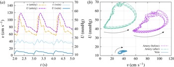
Measurements were performed for more than 40 cases, mostly for the arterial part of the vascular system. The data obtained during operation are pressure and velocity as functions of time. The typical graphs for velocity and pressure in the feeding artery and draining vein are shown in figure 1(a). Note that arterial and venous measurements were never done simultaneously, although graphs for arterial and venous vessels in figure 1(a), correspond to one patient. It is convenient to represent the data on a
 $vp$
-diagram (see figure 1
b). Dashed purple and dash-dotted green diagrams correspond to the measurements taken during one treatment in the afferent of the AVM before and after the embolisation. The
 $vp$
-diagram corresponding to the draining vein is shown in solid blue.
Typical graphs of in vivo measured velocity and pressure of the blood flow in a feeding artery (afferent) and a draining vein of an AVM. (a) Time series. (b)
 $vp$
-diagram in the afferent of the AVM before and after the embolisation, and in the draining vein. Arrows show the direction of movement along the diagrams with time increase.

Several typical features of the
 $vp$
-diagram have been described (Chupakhin et al.
Reference Chupakhin, Cherevko, Khe, Telegina, Krivoshapkin, Orlov, Panarin and Baranov2012):
-
(i) characteristic semicircular shape of the diagram;
-
(ii) conservation of the diagram’s geometry for different measurement points along the vessel;
-
(iii) shift of the diagrams in the upper-left direction on
 $vp$
-plane in the course of the embolisation;
-
(iv) counterclockwise circulation of a point drawing the diagram in arteries during the heartbeat;
-
(v)
$vp$
-diagrams in veins have a similar shape but are reflected with respect to the
$v=p$
line with clockwise circulation of a drawing point during the heartbeat.


The semicircular shape of the diagram indicates the presence of the time shift between the velocity and pressure waves in the vessels. The velocity wave takes the lead over the pressure wave in the arterial part and falls behind in the venous part. The lower smooth part of the arterial diagram in figure 1(b) corresponds to the systole (contraction of the heart muscle), whereas the wavy upper part reflects the diastole (relaxation of the heart muscle). The aim of the paper is to reproduce this behaviour of the
 $vp$
-diagram in the numerical model.
3 How to explain the phase shift?
In the literature concerning the cardiovascular system, the phase shift between the velocity and pressure waves is described in terms of the non-dimensional Womersley number (Caro et al. Reference Caro, Pedley, Schroter and Seed1978). This number governs the relationship between the unsteady and viscous forces for a non-steady flow of viscous fluid in a cylindrical tube.
The velocity of fully developed non-stationary laminar flow of a viscous fluid driven by a time-dependent pressure gradient in a rigid cylindrical tube of fixed radius
 $R$
is given by the following exact solution of Navier–Stokes equations (Gromeka Reference Gromeka1882, Reference Gromeka1883; Womersley Reference Womersley1955):
 $$\begin{eqnarray}w=W(y)\text{e}^{\text{i}{\it\omega}t},\quad \frac{p_{2}-p_{1}}{l}=A\text{e}^{\text{i}{\it\omega}t},\quad y=\frac{r}{R},\text{i}=\sqrt{-1}.\end{eqnarray}$$
Here
 $w$
is the only non-zero velocity component directed along the tube axis,
 $l$
is the tube length and
 $r$
is the distance from the centre of the tube. Function
 $W(y)$
is the real part of the complex function
 $$\begin{eqnarray}W(y)=\frac{A}{{\it\rho}}\frac{1}{\text{i}{\it\omega}}\left(1-\frac{\text{J}_{0}({\it\alpha}y\text{i}^{3/2})}{\text{J}_{0}({\it\alpha}\text{i}^{3/2})}\right),\end{eqnarray}$$
where
 $\text{J}_{0}$
is the Bessel function of the first kind and
 ${\it\rho}$
is the fluid density. The non-dimensional number
 $$\begin{eqnarray}{\it\alpha}=R\sqrt{\frac{{\it\omega}}{{\it\nu}}},\end{eqnarray}$$
is known as the Womersley number (Caro et al.
Reference Caro, Pedley, Schroter and Seed1978). Here
 ${\it\nu}$
is the kinematic viscosity of the fluid.
According to the solution (3.1) the phase shift between the velocity and the pressure wave appears due to the non-zero argument of the complex function
 $W$
as it follows from the representation
 $$\begin{eqnarray}w=|W(y)|\text{e}^{\text{i}({\it\omega}t+\arg W)}.\end{eqnarray}$$
For
 ${\it\alpha}\ll 1$
(narrow tube, high viscosity) the velocity profile is close to Poiseuille flow:
 $$\begin{eqnarray}W(y)=\frac{(1-y^{2}){\it\alpha}^{2}}{4{\it\omega}}+O({\it\alpha}^{4}).\end{eqnarray}$$
The phase shift is negligible since function
 $W$
is real up to the order
 $O({\it\alpha}^{4})$
.
For large
 ${\it\alpha}$
(wider tube, small viscosity) the function
 $W$
has a non-zero imaginary part and the phase shift becomes finite.
In our problem
 $R\approx 0.1$
cm,
 ${\it\omega}\approx 1~\text{s}^{-1}$
,
 ${\it\nu}\approx 3\times 10^{-2}~\text{cm}^{2}~\text{s}^{-1}$
. Hence,
 $$\begin{eqnarray}{\it\alpha}\approx 0.58<1.\end{eqnarray}$$
This calculation implies that in the observed, relatively narrow, blood vessels the velocity profile across the tube can be averaged, as in Poiseuille flow, and the inertial effects described by Gromeka & Womersley’s solution do not seem to play a significant role.
Below, we present a model that gives another explanation of the velocity–pressure time shift and qualitatively describes all of the mentioned features of the
 $vp$
-diagrams.
4 Mathematical model
Let us assume that the brain tissue occupies a region denoted by
 ${\it\Omega}$
. The outer boundary of
 ${\it\Omega}$
is impermeable. The vascular system within the tissue consists of two basins: arterial and venous. There could be several input and output points at the vessel networks, however for simplicity we observe the case of one input
 $O$
at the arterial side and one output
 $E$
at the venous side.
The vascular system plays the role of inner boundary
 ${\it\Gamma}\subset \partial {\it\Omega}$
for the area
 ${\it\Omega}$
. Each vessel’s segment (from one bifurcation to another) is denoted
 ${\it\Gamma}_{j}$
,
 $j=1,\ldots ,N$
, so there are a total of
 $N$
segments in the vessels network and
 ${\it\Gamma}=\bigcup _{j=1}^{N}{\it\Gamma}_{j}$
.
In our model we explicitly resolve the vessel network only up to a certain level of detail. All the vessels of smaller size, as well as the capillary network, are modelled uniformly as a filtration flow within the porous brain tissue. It is assumed that there is a difference between the blood pressure
 $U$
within the vessel and the brain fluid pressure
 $p$
in the capillary network. Pressure
 $U$
is determined only over the vessel network.
4.1 Vascular system
Blood vessels
 ${\it\Gamma}_{j}$
,
 $j=1,\ldots ,N$
, are modelled by (in general, non-straight) tubes of radius
 $R_{j}$
. The position of each vessel
 ${\it\Gamma}_{j}$
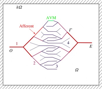
is given and fixed, so that arteries and veins form two (possibly, self-intersecting) vessel networks that do not have direct connections in a ‘healthy’ brain. The schematic two-dimensional (2-D) picture of vessels used in numerical computations is shown in figure 2. This picture qualitatively reconstructs the structure of a real vascular system. The most typical features that were taken into account are the twofold branching of vessels, narrowing of vessels towards the end of the vessel tree and higher connection to the capillary systems for narrower vessels. Modelling of a 3-D ‘real’ vascular system is in principle possible, however it requires a significant effort in terms of the reconstruction of the vessel network, determination of model parameters, verification, etc.
For the numerical experiments we divide all vessels into four levels according to their remoteness from the root of the vessel tree. The number of the level changes at each vessel bifurcation. In the numerical experiments, the properties of each vessel (radius, permeability) depend only on its level in the vessel tree.
The arterial (left) and venous (right) vessel trees. The numbers and the line thickness denote the level of vessels proportional to the distance from the tree root. In numerical experiments all vessels of the same level have equal properties. The AVM is modelled as a direct shunt between the two trees. The afferent is the feeding artery of the AVM.

The fluid flow along each vessel satisfies the continuity equation (for simplicity of notation we omit the index
 $j$
in all individual characteristics of the segment):
 $$\begin{eqnarray}\frac{\partial (S{\it\rho})}{\partial t}+\frac{\partial Q_{v}}{\partial s}=2{\rm\pi}R{\it\rho}q_{l},\quad 0<s<L_{v}.\end{eqnarray}$$
Here
 $S={\rm\pi}R^{2}$
is the sectional area of the vessel,
 $s$
is a local coordinate along the vessel,
 $Q_{v}=S{\it\rho}v_{v}$
is the mass flow rate through the section of the vessel,
 $v_{v}$
is the average fluid velocity,
 $L_{v}$
is the length of the observed segment of the vessel,
 ${\it\rho}$
is a constant fluid density and
 $q_{l}$
is the speed of fluid exchange between the vessel and the brain tissue due to the ‘permeability’ of the vessel’s wall (see the explanation below).
Assuming laminar flow in the vessel and based on the observations of § 3, we take the fluid velocity
 $v_{v}$
from the Hagen–Poiseuille formula:
 $$\begin{eqnarray}v_{v}=-{\it\gamma}\frac{R^{2}}{8{\it\mu}}\frac{\partial U}{\partial s}.\end{eqnarray}$$
Here
 $0<{\it\gamma}\leqslant 1$
is the imperfection coefficient that takes into account possible additional resistance to the flow due to unrecorded factors. For simplicity we assume the vessel radius to be time independent, although the case of a pressure-dependent radius
 $R(U)$
may also be treated with our approach.
4.2 The brain tissue
The microcapillary system is a dense network of thin (
 ${\approx}1~{\rm\mu}\text{m}$
) blood vessels. It is impossible to resolve this network explicitly, so we substitute it with a porous material with a given porosity
 $m$
and permeability
 $k$
satisfying Darcy’s law. The blood is modelled as a Newtonian fluid with dynamic viscosity
 ${\it\mu}$
equal to approximately four times the viscosity of water.
The ‘porosity’ of the tissue
 $m$
is the relative volume of the tissue occupied by a capillary network. In our model we take into account the elasticity of the tissue by assuming the porosity to be a linear function of the fluid pressure
 $$\begin{eqnarray}m=m_{0}(1+{\it\varepsilon}(p-p_{0})),\end{eqnarray}$$
where
 $m_{0}$
and
 $p_{0}$
are the reference porosity and pressure, and
 ${\it\varepsilon}$
is the elastic capacity coefficient. For estimation of
 ${\it\varepsilon}$
we assume that an increase in pressure of
 $20$
mmHg leads to a 1 % increase in
 $m$
, which gives
 ${\it\varepsilon}=1/2000~\text{mmHg}^{-1}=3.75\times 10^{-6}~\text{Pa}^{-1}$
.
A proper estimate of the permeability of the tissue should involve formal averaging or homogenization, for example as proposed in the paper by Penta, Ambrosi & Quarteroni (Reference Penta, Ambrosi and Quarteroni2015). In our work, we use a simple approach based on the scaling argument due to the analogy of the Poiseuille law for the averaged velocity
 $\boldsymbol{q}$
driven by a pressure gradient in one capillary of radius
 $r$
with Darcy’s law for the tissue:
 $$\begin{eqnarray}\boldsymbol{q}=-\frac{r^{2}}{8{\it\mu}}\boldsymbol{{\rm\nabla}}p=-\frac{k}{{\it\mu}m_{0}}\boldsymbol{{\rm\nabla}}p.\end{eqnarray}$$
Hence,
 $$\begin{eqnarray}k\approx r^{2}m_{0}/8.\end{eqnarray}$$
By taking
 $r\approx 5~{\rm\mu}\text{m}$
and
 $m_{0}=0.2$
we obtain
 $k\approx 6.25\times 10^{-9}~\text{cm}^{2}$
.
The equation of one-phase filtration in the tissue of the brain follows from the mass continuity equation and Darcy’s law in the form
 $$\begin{eqnarray}\frac{\partial (m{\it\rho})}{\partial t}-\text{div}\,\left({\it\rho}\frac{k}{{\it\mu}}\boldsymbol{{\rm\nabla}}p\right)=0,\quad \boldsymbol{x}\in {\it\Omega}\setminus {\it\Gamma}.\end{eqnarray}$$
Equations (4.1) and (4.6) are connected by boundary conditions on the vessel walls.
4.3 Vessel–tissue interaction
The interaction of the blood flow in the vessels with the filtration flow in the brain tissue is modelled by a boundary condition of the third kind, implying that the velocity of the fluid exchange is proportional to the pressure difference on the adjacent sides of the vessel:
 $$\begin{eqnarray}q_{j}=-\left(\frac{k}{{\it\mu}}\frac{\partial p}{\partial {\it\nu}}\right)_{{\it\Gamma}_{j}}={\it\kappa}_{j}(p|_{{\it\Gamma}_{j}}-U),\quad j=1,\ldots ,N.\end{eqnarray}$$
Here
 ${\it\nu}$
is the outer (with respect to the area
 ${\it\Omega}$
) normal to the boundary
 ${\it\Gamma}_{j}$
and
 $q_{l}$
specifies the velocity of the fluid exchange between the vessel and the tissue due to the unresolved network of arterioles and venules binding the main network of vessels to the microcapillary system of the brain. From mechanical considerations,
 $q_{l}$
is negative for the arterial part and positive for the venous part. The coefficients
 ${\it\kappa}_{j}$
determine the ‘permeability’ of the vessel walls. Here, the permeability which is proportional to the density of the unresolved networks of arterioles and venules. We take the permeability to be smaller for wider vessels and larger for the thinner ones.
From (4.1), (4.2) and (4.7) for constant vessel radius we obtain the equation for the pressure distribution within each blood vessel in the form
 $$\begin{eqnarray}\frac{{\it\gamma}_{j}{\rm\pi}R_{j}^{4}}{8{\it\mu}}\frac{\partial ^{2}U}{\partial s^{2}}=-2{\rm\pi}R_{j}{\it\kappa}_{j}(p|_{{\it\Gamma}_{j}}-U),\quad 0<s<L_{vj},\quad j=1,\ldots ,N.\end{eqnarray}$$
Equation (4.8) for each segment is complemented by the boundary conditions:
-
(i) at the each joint of the segments function
$U$
is continuous; -
(ii) the total flow rate through any joint is equal to zero;
-
(iii) at the input
$O$
and the output
$E$
of the system, either the flow rate or the pressure is given; -
(iv) at the ends of the most distant branches of the vessels that do not have any further connections the flow rate is zero.


Henceforth, these boundary conditions are referred to as b.c. (i)–(iv). Normally, we prescribe the flow rate at the input
 $O$
and the pressure at the output
 $E$
or vice versa. The condition of zero flow rate at the ends of the ‘branches’ implies that all fluid is drained into the capillary system.
4.4 Weak formulation of the problem
Let us write the weak statement of the problem. Due to the fluid incompressibility
 ${\it\rho}=\text{const}.$
from (4.3) we have
 $$\begin{eqnarray}\displaystyle \frac{\partial m}{\partial t}=\frac{\partial }{\partial t}(m_{0}(1+{\it\varepsilon}(p-p_{0})))=m_{0}{\it\varepsilon}\frac{\partial p}{\partial t}.\end{eqnarray}$$
Equation (4.6) gives
 $$\begin{eqnarray}m_{0}{\it\varepsilon}\frac{\partial p}{\partial t}-\text{div}\,\left(\frac{k}{{\it\mu}}\boldsymbol{{\rm\nabla}}p\right)=0.\end{eqnarray}$$
By multiplication of this equation to an arbitrary function
 ${\it\psi}(\boldsymbol{x})$
and integration over the domain
 ${\it\Omega}$
we have
 $$\begin{eqnarray}\displaystyle 0 & = & \displaystyle \int _{{\it\Omega}}{\it\psi}\left(m_{0}{\it\varepsilon}\frac{\partial p}{\partial t}-\text{div}\,\left(\frac{k}{{\it\mu}}\boldsymbol{{\rm\nabla}}p\right)\right)\,\text{d}{\it\Omega}\nonumber\\ \displaystyle & = & \displaystyle \int _{{\it\Omega}}\left(m_{0}{\it\varepsilon}{\it\psi}\frac{\partial p}{\partial t}-\text{div}\,\left({\it\psi}\frac{k}{{\it\mu}}\boldsymbol{{\rm\nabla}}p\right)+\frac{k}{{\it\mu}}\boldsymbol{{\rm\nabla}}{\it\psi}\boldsymbol{{\rm\nabla}}p\right)\,\text{d}{\it\Omega}\nonumber\\ \displaystyle & = & \displaystyle \int _{{\it\Omega}}\left(m_{0}{\it\varepsilon}{\it\psi}\frac{\partial p}{\partial t}+\frac{k}{{\it\mu}}\boldsymbol{{\rm\nabla}}{\it\psi}\boldsymbol{{\rm\nabla}}p\right)\,\text{d}{\it\Omega}-\frac{k}{{\it\mu}}\int _{\partial {\it\Omega}}{\it\psi}\frac{\partial p}{\partial {\it\nu}}\,\text{d}S.\end{eqnarray}$$
The boundary integral can be transformed according to (4.7) and due to the no-flow condition over the outer boundary of
 ${\it\Omega}$
:
 $$\begin{eqnarray}\left.\frac{\partial p}{\partial {\it\nu}}\right|_{\partial {\it\Omega}\setminus {\it\Gamma}}=0.\end{eqnarray}$$
This leads to the weak formulation of the equation for the fluid pressure within the brain tissue:
 $$\begin{eqnarray}\int _{{\it\Omega}}\left(m_{0}{\it\varepsilon}{\it\psi}\frac{\partial p}{\partial t}+\frac{k}{{\it\mu}}\boldsymbol{{\rm\nabla}}{\it\psi}\boldsymbol{{\rm\nabla}}p\right)\,\text{d}{\it\Omega}+\mathop{\sum }_{j=1}^{N}2{\rm\pi}R_{j}{\it\kappa}_{j}\int _{{\it\Gamma}_{j}}{\it\psi}(p-U)\,\text{d}s=0.\end{eqnarray}$$
Multiplication of (4.8) to an arbitrary, smooth over
 ${\it\Gamma}$
, function
 ${\it\eta}(\boldsymbol{x})$
and integration over both networks of vessels leads to the following integral relation:
 $$\begin{eqnarray}\displaystyle 0 & = & \displaystyle \mathop{\sum }_{j=1}^{N}\int _{{\it\Gamma}_{j}}{\it\eta}\left(\frac{{\it\gamma}_{j}{\rm\pi}R_{j}^{4}}{8{\it\mu}}\frac{\partial ^{2}U}{\partial s^{2}}+2{\rm\pi}R_{j}{\it\kappa}_{j}(p-U)\right)\,\text{d}s\nonumber\\ \displaystyle & = & \displaystyle \mathop{\sum }_{j=1}^{N}\left.\frac{{\it\gamma}_{j}{\rm\pi}R_{j}^{4}}{8{\it\mu}}{\it\eta}\frac{\partial U}{\partial s}\right|_{\partial {\it\Gamma}_{j}}-\mathop{\sum }_{j=1}^{N}\int _{{\it\Gamma}_{j}}\left(\frac{{\it\gamma}_{j}{\rm\pi}R_{j}^{4}}{8{\it\mu}}\frac{\partial {\it\eta}}{\partial s}\frac{\partial U}{\partial s}-2{\rm\pi}R_{j}{\it\kappa}_{j}{\it\eta}(p-U)\right)\,\text{d}s.\end{eqnarray}$$
Every term in the first sum in (4.14) is proportional to the flow rate at the end of each vessel segment
 ${\it\Gamma}_{j}$
. Due to mass conservation, all flow rates at points of intersection of the segments cancel out. We assume flow rates at the end of the narrowest segments of each branch of vessels to be zero. The only flow rates remaining in this formula are the rates
 $Q_{a}(t)$
and
 $Q_{v}(t)$
at the roots
 $O$
and
 $E$
of the arterial and venous vessel trees. Hence, the equation for the blood pressure within the vessels reads
 $$\begin{eqnarray}\mathop{\sum }_{j=1}^{N}\int _{{\it\Gamma}_{j}}\left(\frac{{\it\gamma}_{j}{\rm\pi}R_{j}^{4}}{8{\it\mu}}\frac{\partial {\it\eta}}{\partial s}\frac{\partial U}{\partial s}-2{\rm\pi}R_{j}{\it\kappa}_{j}{\it\eta}(p-U)\right)\,\text{d}s-{\it\eta}(O)Q_{a}(t)-{\it\eta}(E)Q_{v}(t)=0.\end{eqnarray}$$
Let us define the space
 ${\mathcal{U}}=\{U\in W^{1,2}({\it\Gamma})\mid \text{b.c. (i)}{-}\text{(iv)}\}$
. Now the weak formulation of the problem reads as follows: at any time
 $t\in [0,T]$
we find functions
 $p\in W^{1,2}({\it\Omega}\setminus {\it\Gamma})$
and
 $U\in {\mathcal{U}}$
such that (4.13), (4.15) are satisfied for every
 ${\it\psi}\in C^{1}({\it\Omega}\setminus {\it\Gamma})$
and
 ${\it\eta}\in C^{1}({\it\Gamma})$
and
 $p=p_{0}\in L^{2}({\it\Omega}\setminus {\it\Gamma})$
,
 $U=U_{0}\in L^{2}({\it\Gamma})$
at
 $t=0$
.
4.5 Dimensionless form
Let us introduce the following dimensionless variables:
 $$\begin{eqnarray}t^{\prime }=t/T,\quad p^{\prime }=p/p_{\ast },\quad U^{\prime }=U/p_{\ast },\quad q^{\prime }=TQ/(LR^{2}),\quad \boldsymbol{x}^{\prime }=\boldsymbol{x}/L,\quad r_{j}^{\prime }=R_{j}/R.\end{eqnarray}$$
Set of parameters for the numerical experiment.

Here
 $T$
,
 $L$
,
 $R$
and
 $p_{\ast }$
are some characteristic scales of time, size of the area
 ${\it\Omega}$
, vessel radius and blood pressure. Writing the problem (4.13), (4.15) in dimensionless variables gives (primes are omitted)
 $$\begin{eqnarray}\displaystyle & \displaystyle \int _{{\it\Omega}}\left(a_{1}{\it\psi}\frac{\partial p}{\partial t}+a_{2}\boldsymbol{{\rm\nabla}}{\it\psi}\boldsymbol{{\rm\nabla}}p\right)\,\text{d}{\it\Omega}+\mathop{\sum }_{j=1}^{N}a_{3j}\int _{{\it\Gamma}_{j}}{\it\psi}(p-U)\,\text{d}s=0, & \displaystyle\end{eqnarray}$$
 $$\begin{eqnarray}\displaystyle & \displaystyle \mathop{\sum }_{j=1}^{N}\int _{{\it\Gamma}_{j}}\left(a_{4j}\frac{\partial {\it\eta}}{\partial s}\frac{\partial U}{\partial s}-a_{3j}{\it\eta}(p-U)\right)\,\text{d}s-{\it\eta}(O)q_{a}(t)-{\it\eta}(E)q_{v}(t)=0, & \displaystyle\end{eqnarray}$$
 $$\begin{eqnarray}\displaystyle {\it\delta}=\frac{R}{L},\quad a_{1}=\frac{m_{0}{\it\varepsilon}p_{\ast }}{{\it\delta}^{2}},\quad a_{2}=\frac{Tp_{\ast }k}{{\it\mu}R^{2}},\quad a_{3j}=\frac{2{\rm\pi}r_{j}{\it\kappa}_{j}Tp_{\ast }}{R},\quad a_{4j}=\frac{{\it\gamma}_{j}{\rm\pi}Tp_{\ast }{\it\delta}^{2}r_{j}^{4}}{{\it\mu}}. & & \displaystyle \nonumber\\ \displaystyle & & \displaystyle\end{eqnarray}$$
With the characteristic values of parameters (Caro et al. Reference Caro, Pedley, Schroter and Seed1978; Pedley Reference Pedley1980)
 $$\begin{eqnarray}\displaystyle \left.\begin{array}{@{}c@{}}T=1s,\quad L=10~\text{cm},\quad R=0.1~\text{cm},\quad m_{0}=0.1,\quad {\it\mu}=10^{-2}~\text{g}~\text{cm}^{-1}~\text{s}^{-1},\\ p_{\ast }=10^{3}~\text{g}~\text{cm}^{-1}~\text{s}^{-2},\quad {\it\varepsilon}=10^{-6}~\text{cm}~\text{s}^{2}~\text{g}^{-1},\quad k=10^{-9}~\text{cm}^{2},\\ {\it\kappa}=k/({\it\mu}R)=10^{-6}~\text{cm}^{2}~\text{s}~\text{g}^{-1}\end{array}\right\}\quad & & \displaystyle\end{eqnarray}$$
we obtain the following values of dimensionless coefficients:
 $$\begin{eqnarray}\displaystyle {\it\delta}=10^{-2},\quad a_{1}=1,\quad a_{2}=10^{-2},\quad a_{3j}=2{\rm\pi}\times 10^{-2},\quad a_{4j}={\it\gamma}_{j}{\rm\pi}\times 10.\qquad & & \displaystyle\end{eqnarray}$$
5 Numerical experiment
In order to reproduce numerically the described qualitative characteristics of the cerebral blood flow we use a 2-D model of the vessel net. As shown below, the proposed model demonstrates the phase shift between the pressure and velocity waves, as well as a suitable interval for the pressures and velocities. More accurate simulations would require reconstruction of the full 3-D model of the vessels up to a certain level of detail, selection of parameters of the vessels and of the brain tissue, etc.
5.1 Construction of the vessel net
For the numerical experiment we use the set of parameters listed in table 1. The area
 ${\it\Omega}$
is taken as a rectangle
 $L\times L$
containing the vessel network in its centre. Blood vessels
 ${\it\Gamma}_{j}$
are represented by line segments comprising the two vessel trees as shown in figure 2. At the input
 $O$
we specify a flow rate, at the output
 $E$
we set a given pressure. Graphs of the velocity
 $v(O)$
and the pressure
 $U(E)$
used in the experiment are taken as in figure 1(a). Note that specification of the pressure at point
 $O$
and the flow rate at point
 $E$
gives qualitatively similar results.
For simplicity we divided all vessels into levels: the level number increases after each bifurcation (see figure 2). All vessels from the same level have the same properties (radius, wall permeability, etc). For calculations we take the radii of the first level for the arterial and venous networks to be 1 mm and 1.5 mm respectively. The radii of the vessels of every next level are taken to be 1.5 times smaller than the radii at the preceding level.
For the modelling of the AVM we connect the upper segments of the arterial and venous networks with a shunt, as shown in figure 2. Pressure and velocity are calculated in the afferent artery (see figure 2) and at the point
 $E$
at the output of the venous network. The radius of the AVM shunt is taken as 0.5 mm before the embolisation and
 $0.5\times 10^{-6}$
mm after the embolisation.
As an initial condition we use uniform pressure
 $p=0$
and
 $U=0$
. The calculations are carried out with a time step equivalent to
 $0.01$
s. After some initial period of time (approximately 2 s) the system reaches a periodic state where the pressure waves repeat at every pulsation of the input and output data.
5.2 Numerical method
The formulated problem was solved by a finite element method using the freely distributed package FreeFEM++ (Hecht Reference Hecht2012). For the numerical calculations we adopted a triangular mesh with quadratic finite elements. The number of mesh vertices is equal to 50 over each of the outer boundaries and approximately 15 over each of the vessel segments (the particular number depends on the vessel length). The overall number of mesh vertices is equal to 6293. The second-order convergence of the method was checked by consequent calculations on denser meshes.
The time derivative is approximated by finite differences:
 $\partial p/\partial t\approx (p^{n+1}-p^{n})/{\it\tau}$
where
 ${\it\tau}$
is the time step. The upper index denotes the time instant:
 $p^{n}=p(t_{n},\boldsymbol{x})$
,
 $t_{n}=n{\it\tau}$
. Time iterations are performed using the first-order backward (implicit) Euler method. Due to the unconditional stability of the method, the value of the time step
 ${\it\tau}$
does not depend on the characteristic diameter of the mesh cells.
5.3 Results of calculations
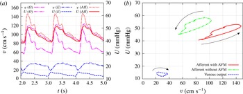
Computational results for the velocity and pressure at different points of the flow domain. (a) Time series at the roots of the arterial (
 $O$
) and the venous (
 $E$
) trees, and in the afferent for the case with the AVM. (b)
 $vp$
-diagram in the afferent and at the root
 $E$
of the venous tree before and after the embolisation. Arrows show the direction of circulation along the diagrams.

The calculations of pressure and velocity at points
 $O$
,
 $E$
and in the afferent in the periodic state of the system in the presence of the AVM are shown in figure 3(a). Figure 3(b), demonstrates the
 $vp$
-diagram for the before and after embolisation states measured at the afferent and at the output of the venous network. The venous diagram remains almost undistinguishable in both states, whereas the arterial one shifts in the upper-left direction in correspondence with the experimental data. The semicircular shape of the diagram qualitatively coincides with the experimental one shown in figure 1(b). More importantly, the direction of circulation along the diagram during the pulsation coincides with the experimental one, i.e. it is counterclockwise in the arterial part and clockwise in the venous part.
Another calculation with a given pressure at the input and flow rate at the output has produced very similar results with the same qualitative features. This implies that the phase shift and the order of waves do not depend on the type of boundary conditions and are determined by the position of the vessels relative to the capillary net. Among another observations concerning the AVM modelling we noticed that presence of the low-resistant connection between arterial and venous networks due to the AVM tends to equate pressure in both parts of the system, which is harmful for both types of vessels and can be observed to be one of the most common causes of the rupture.
The calculations demonstrate that the capillary system, represented in the model as a porous medium, acts as a strong dissipative mechanism. In a healthy vascular system (without AVM) it suppresses pulse waves in such a way that pressure fluctuations are negligible within a capillary. There is no direct connection between pressure waves in arteries and veins, hence the type of boundary conditions (flux or pressure) at the input and output of the system do not change the flow pattern. The phase shift between the velocity and pressure waves is regulated by the relative position of the dissipative part to the source or sink of the fluid. This observation is supported by in vivo measurements and by the analytical solution (see below).
The presence of the AVM tends to equalize pressures in the arterial part (where the flux at
 $O$
is specified) and in the venous part (where the pressure at
 $E$
is given), however, the overall resistance of the system does not change. The pressure waves in the arterial part are damped although the total flux is conserved. Therefore, the venous part acts, in a sense, independently from the arterial part. This observation explains the coincidence of the venous
 $vp$
-diagram for cases before and after embolisation.
6 Theoretical explanation of the time shift
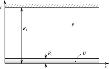
In order to give a theoretical explanation of the observed time shift between the velocity and pressure waves in the vessel we observe the simplest configuration of one infinite vessel within a cylindrical porous medium. The vessel of radius
 $R_{0}$
is located along the positive
 $Ox$
-axis. The porous tissue forms a cylinder of radius
 $R_{1}$
. On the outer wall of the tissue, the no-flow condition is specified (see figure 4).
Modelling configuration for the analytical prediction of the time shift between velocity and pressure waves. A single vessel of radius
 $R_{0}$
is immersed in a cylindrical porous medium of radius
 $R_{1}$
. The fluid pressure in the vessel and in the medium are
 $U$
and
 $p$
respectively.

The mathematical statement of the problem is the following. The equation for the fluid pressure in the tissue is
 $$\begin{eqnarray}\frac{\partial p}{\partial t}={\it\tau}\left(\frac{\partial ^{2}p}{\partial x^{2}}+\frac{1}{r}\frac{\partial }{\partial r}\left(r\frac{\partial p}{\partial r}\right)\right).\end{eqnarray}$$
Here
 ${\it\tau}=k/({\it\mu}m_{0}{\it\varepsilon})$
. The boundary conditions on the vessel’s wall are
 $$\begin{eqnarray}\quad \text{at }r=R_{0}:\left\{\begin{array}{@{}ll@{}}\displaystyle \frac{\partial ^{2}U}{\partial x^{2}}+{\it\sigma}(p-U)=0,\quad \quad & \displaystyle {\it\sigma}=\frac{16{\it\mu}{\it\kappa}}{{\it\gamma}R_{0}^{3}}\\ \displaystyle \frac{\partial p}{\partial r}={\it\zeta}(p-U),\quad & \displaystyle {\it\zeta}=\frac{{\it\mu}{\it\kappa}}{k}.\end{array}\right.\end{eqnarray}$$
The no-flow condition on the outer cylinder reads
 $$\begin{eqnarray}\text{ at }r=R_{1}:\quad \frac{\partial p}{\partial r}=0.\end{eqnarray}$$
We construct the solution in the form of a single wave packet:
 $$\begin{eqnarray}U=\text{e}^{\text{i}{\it\omega}t-kx},\quad p=\text{e}^{\text{i}{\it\omega}t-kx}P(r),\end{eqnarray}$$
where
 $k$
is some complex wavenumber. Generally,
 $k$
has a non-zero real part
 $\text{Re}(k)\neq 0$
. In the physically meaningful solution
 $\text{Re}(k)\leqslant 0$
for
 $x>0$
(upstream source) and
 $\text{Re}(k)\geqslant 0$
for
 $x<0$
(downstream sink). In the cerebral vessels the overall flow is directed from the arteries to the veins, hence the upstream source corresponds to the arterial part and the downstream sink describes the venous part.
Representation of the solution for
 $p$
in (6.4) can be written as follows:
 $$\begin{eqnarray}p=\text{e}^{\text{i}({\it\omega}t+\arg (P))-kx}|P(r)|.\end{eqnarray}$$
This implies that
 $\text{arg}(P)/{\it\omega}$
specifies the phase shift for the wave in the porous tissue with respect to the wave in the vessel.
The fluid velocity in the vessel is given by formula (4.2) which is
 $$\begin{eqnarray}v_{v}=-\frac{{\it\gamma}R^{2}}{8{\it\mu}}\frac{\partial U}{\partial x}=-\frac{{\it\gamma}R^{2}|k|}{8{\it\mu}}\text{e}^{\text{i}({\it\omega}t+\arg (k))-kx}.\end{eqnarray}$$
Therefore, the phase shift of the velocity wave with respect to the pressure wave is determined by the
 $\arg (k)/{\it\omega}$
. A positive value of
 $\arg (k)$
implies a shift of the graph of function
 $v_{v}$
to the left, i.e. the velocity wave takes the lead over the pressure wave (arterial scenario). On the contrary, a negative value of
 $\arg (k)$
shifts the graph of
 $v_{v}$
to the right and the pressure wave runs ahead of the velocity wave (venous scenario).
Combining the two observations concerning signs of
 $\text{Re}(k)$
and
 $\arg (k)$
we conclude that there should be
 $0\leqslant \arg (k)\leqslant {\rm\pi}/2$
in the arterial part and
 ${\rm\pi}\leqslant \arg (k)\leqslant 3{\rm\pi}/2$
in the venous part. It remains to show the existence of solutions of the problem with wavenumber
 $k$
in the required sectors of the complex plane.
Substitution of representation (6.4) into (6.1) gives
 $$\begin{eqnarray}\frac{\text{i}{\it\omega}}{{\it\tau}}P=k^{2}P+\frac{1}{r}\frac{\partial }{\partial r}(rP^{\prime }(r)).\end{eqnarray}$$
Integration of the latter ordinary differential equation gives the following solution for
 $P$
:
 $$\begin{eqnarray}P=c_{1}\text{J}_{0}({\it\delta}r)+c_{2}Y_{0}({\it\delta}r),\quad {\it\delta}=\sqrt{k^{2}-\frac{\text{i}{\it\omega}}{{\it\tau}}}.\end{eqnarray}$$
Henceforth,
 $\text{J}_{i}$
and
 $\text{Y}_{i}$
,
 $i=0,1$
, are Bessel functions of the first and second kind. The no-flow condition (6.3) after cancellation of insufficient multiplier yields
 $$\begin{eqnarray}c_{1}\text{J}_{1}({\it\delta}R_{1})+c_{2}\text{Y}_{1}({\it\delta}R_{1})=0.\end{eqnarray}$$
Hence,
 $P$
can be represented as
 $$\begin{eqnarray}P=c(\text{Y}_{1}({\it\delta}R_{1})\text{J}_{0}({\it\delta}r)-\text{J}_{1}({\it\delta}R_{1})\text{Y}_{0}({\it\delta}r)),\end{eqnarray}$$
with an arbitrary constant
 $c$
. Substitution into the boundary conditions (6.2) leads to the equations
 $$\begin{eqnarray}\displaystyle k^{2}+{\it\sigma}(P(R_{0})-1)=0, & & \displaystyle\end{eqnarray}$$
 $$\begin{eqnarray}\displaystyle P^{\prime }(R_{0})={\it\zeta}(P(R_{0})-1). & & \displaystyle\end{eqnarray}$$
 $c$
in the form
 $$\begin{eqnarray}c=\frac{k^{2}{\it\zeta}}{{\it\delta}{\it\sigma}{\it\Delta}},\quad {\it\Delta}=Y_{1}({\it\delta}R_{1})J_{1}({\it\delta}R_{0})-J_{1}({\it\delta}R_{1})Y_{1}({\it\delta}R_{0}).\end{eqnarray}$$
Finally, we obtain the equation for the complex wavenumber
 $k$
:
 $$\begin{eqnarray}\displaystyle g(k) & = & \displaystyle k^{2}{\it\zeta}(Y_{1}({\it\delta}R_{1})\text{J}_{0}({\it\delta}r)-J_{1}({\it\delta}R_{1})Y_{0}({\it\delta}r))\nonumber\\ \displaystyle & & \displaystyle +\,{\it\delta}{\it\sigma}(Y_{1}({\it\delta}R_{1})J_{1}({\it\delta}R_{0})-J_{1}({\it\delta}R_{1})Y_{1}({\it\delta}R_{0}))\left(1-\frac{k^{2}}{{\it\sigma}}\right)=0.\end{eqnarray}$$
Note that the function
 $g$
depends only on
 $k^{2}$
, hence solutions of (6.33) are symmetrical with respect to the origin
 $k=0$
, i.e. there are two sets of solutions for
 $\text{Re}(k)>0$
and
 $\text{Re}(k)<0$
that coincide after rotation on
 ${\rm\pi}$
in the complex plane.
Equation (6.33) for the complex wavenumber
 $k$
was solved numerically using Wolfram Mathematica©. The following set of parameters was used:
 $$\begin{eqnarray}{\it\omega}=1,\quad {\it\sigma}=1,\quad {\it\tau}=1,\quad {\it\zeta}=1,\quad R_{0}=0.1,\quad R_{1}=1.\end{eqnarray}$$
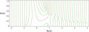
Zero-level lines for real and imaginary parts of the function
 $g$
are shown in figure 5. Only half of the complex plane is shown, graphs in the lower half-plane are symmetrical with respect to the origin
 $k=0$
. The qualitative picture of zero-level lines in figure 5 is stable to variation of the problem parameters. Intersections of the lines give the roots of (6.33) for
 $k$
. From this numerical experiment one can conclude the existence of a (probably, countable) set of roots
 $k$
of (6.33) with
 $0<\arg (k)<{\rm\pi}/2$
and a symmetrical set of roots with
 ${\rm\pi}<\arg (k)<3{\rm\pi}/2$
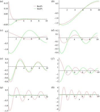
. Numerical values of the several first roots of (6.33) are given in table 2. Graphs of the real and imaginary parts of function
 $P(r)$
for the corresponding roots
 $k_{j}$
are shown in figure 6.
Zero-level lines for real (dashed red) and imaginary (solid green) parts of the function
 $g(k)$
. Intersections of the lines give the complex roots
 $k$
of (6.33).

Numerical values of some roots of (6.33).

Real (dashed red) and imaginary (solid green) parts of the function
 $P(r)$
for some roots
 $k_{j}$
of (6.33): (a)
 $k=0.798876+0.0528743i$
; (b)
 $k=0.763257+0.656872i$
; (c)
 $k=0.898953+0.550532i$
; (d)
 $k=1.13493+0.421902i$
; (e)
 $k=1.40215+0.351927i$
; (f)
 $k=1.67104+0.290608i$
; (g)
 $k=2.0127+0.255911i$
; (h)
 $k=3.24419+0.155055i$
.

From the observations above we conclude that the roots
 $k=k_{i}$
shown in figure 5 correspond to the upstream source with the lead of the velocity wave (arterial behaviour), whereas the symmetrical roots reflect the downstream sink with the lead of the pressure wave (venous behaviour). This remark explains the difference in the direction of circulation of the arterial and venous diagrams.
7 Discussion and conclusion
Mathematical description of blood flow is often based on the 1-D model derived from the Navier–Stokes equations by averaging over the cross-section of the blood vessel. Analytical investigations of the equations governing flows in a tube with rigid and elastic walls can be found in works by Gromeka (Reference Gromeka1882, Reference Gromeka1883) and Womersley (Reference Womersley1955). A number of mathematical models for blood flow simulation have since been developed (Caro et al. Reference Caro, Pedley, Schroter and Seed1978; Pedley Reference Pedley1980).
Models based on the mass and momentum balance laws for viscous fluid flow in a net of collapsible tubes in a 1-D approximation were proposed in Sherwin et al. (Reference Sherwin, Formaggia, Peiro and Franke2003a ,Reference Sherwin, Franke, Peiró and Parker b ), Formaggia, Quarteroni & Veneziani (Reference Formaggia, Quarteroni and Veneziani2009) and Müller and Toro (Reference Müller and Toro2014). In Reymond et al. (Reference Reymond, Merenda, Perren, Rüfenacht and Stergiopulos2007, Reference Reymond, Merenda, Perren, Rüfenacht and Stergiopulos2009, Reference Reymond, Bohraus, Perren, Lazeyras and Stergiopulos2011) a 1-D model of the cardiovascular system was developed. The authors obtained a physiologically relevant model of the entire system, including the cerebral artery network, which is coupled to a heart model. A comparison of pulse wave propagation in a 1-D nonlinear model governing blood flow in Voigt-type viscoelastic arteries with in vitro measurements was carried out by Alastruey et al. (Reference Alastruey, Khir, Matthys, Segers, Sherwin, Verdonck, Parker and Peiró2011). Being suitable for description of the blood flow in relatively large vessels, these models do not account for the flow in the surrounding tissue.
Mathematical modelling of AVM haemodynamics has been tackled in several works. Local haemodynamics in the AVM nidus is considered in works by Smith and Jones (Reference Smith and Jones2000, Reference Smith and Jones2003). Various branching configurations were studied, including one-to-many branching with different flow rates. Propagation of the embolisation agent was studied in White and Smith (Reference White and Smith2013). The authors used a two-phase flow model to simulate viscous droplet motion through a bifurcation or multifurcation point.
Global hydrodynamic properties of the AVM were studied in papers by Guglielmi (Reference Guglielmi2008), Litao, Pilar-Arceo & Legaspi (Reference Litao, Pilar-Arceo and Legaspi2012) and Telegina, Chupakhin & Cherevko (Reference Telegina, Chupakhin and Cherevko2013). Their approach was based on the electric circuit or hydraulic network analogy and allowed investigation of the stationary hydraulic characteristics of the blood flow. In particular, based on an electrical network analogy, Guglielmi (Reference Guglielmi2008) analysed the embolisation treatment procedure for two models of AVMs: a low-flow and a high-flow model. Their study shows that occlusion of the arterial feeders results in a decrease in both the arterial pressure and the flow in the nidus, while occlusion of the draining vein leads to a significant increase in blood pressure in the AVM nidus. Moreover, occlusion of the high-flow fistulous component in high-flow AVMs considerably increases the blood flow through the healthy brain.
Using the electrical network model, Litao et al. (Reference Litao, Pilar-Arceo and Legaspi2012) found the influence of the presence of the multiple compartments in the AVM on a pressure drop across the nidus. They showed that the transnidal pressure decreases with an increase in the number of the AVM compartments. In the paper by Telegina et al. (Reference Telegina, Chupakhin and Cherevko2013) different scenarios for embolisation based on a hydraulic analogy, which is similar to the electrical analogy, were studied. The general recommendations were that a treatment should start with occlusion of a fistula compartment (i.e. a shunt represented by a vessel of relatively large diameter) if present, following the embolisation of racemose AVM compartments (consisting of a chaotic net of small-diameter vessels). The above-mentioned findings agree with the common medical view on the AVM heamodynamics.
In Papapanayotou, Cherruault & De La Rochefoucauld (Reference Papapanayotou, Cherruault and De La Rochefoucauld1990), by using 1-D mass and momentum balance laws, the authors developed a model describing the influence of the AVM on the distribution of fluxes within the vessels of the Willis circle. Numerical experiments show that the volume flux in the AVM could be significantly reduced by reduction of the feeding artery and obstruction of the anterior communicating artery.
Simulation of the AVM haemodynamics was performed by Simakov et al. (Reference Simakov, Gorodnova, Chupakhin and Khe2013). The authors applied a previously developed global blood circulation model to flow in the AVM described as a graph of vessels with some arbitrary connections (Abakumov et al. Reference Abakumov, Ashmetkov, Esikova, Koshelev, Mukhin, Sosnin, Tishkin, Favorskii and Khrulenko2000; Kholodov Reference Kholodov, Belotserkovskii and Kholodov2001). The governing system was a 1-D hyperbolic system of two differential equations: conservation laws for mass and momentum. The compliance of the vessel wall was incorporated via the ‘equation of state’: a relation between the pressure and the cross-sectional area. The embolisation procedure was modelled by an increase of the hydraulic resistance of the afferent (i.e. incoming) vessels.
One-dimensional models were successfully applied to both arterial and venous vessel networks. In Qureshi et al. (Reference Qureshi, Vaughan, Sainsbury, Johnson, Peskin, Olufsen and Hill2014) such a model was used for a description of the pulmonary circulation. Blood flow in ‘large’ vessels up to the fourth generation from the inlet was governed by a 1-D model, while the mirror terminal ends of the arterial and venous nets were connected through a vessel bed. Exploiting the smallness of the vessels and linearising the 1-D governing equation, the authors constructed
 $2\times 2$
admittance matrices relating the flows and pressures at the outlet of the arterial and the inlet of the venous networks. Thus, the blood flow through the capillary bed was effectively resolved by relations at the terminal ends of the arterial and venous trees. We note that there should be a one-to-one mapping between corresponding terminal ends.
An approach very close to ours was applied by Cattaneo and Zunino (Reference Cattaneo and Zunino2014) for modelling of the flow in capillaries and tissue interstitium. Their model comprised a 1-D network of microvessels immersed in a 3-D porous interstitial medium. In contrast to our work, the authors addressed the problem of microcirculation and interstitial flow interaction, including lymphatic drainage. Keeping in mind mass transport and drug delivery, the authors showed the ability of the model to describe the flow patterns in healthy and tumorous tissues (i.e. in 3-D domains of the problem’s geometry). Mathematical correctness of a similar problem with the coupling of 3-D and 1-D flows was studied by D’Angelo and Quarteroni (Reference D’Angelo and Quarteroni2008), where the well-posedness of the coupled problem was established in suitable functional spaces. This allows one to perform a convergence analysis of finite element schemes.
In our paper we propose a model of blood propagation within two trees of relatively narrow vessels (arterial and venous) connected by a capillary network. The model is applicable to the numerical simulation of local cerebral haemodynamics and, in particular, can be used for modelling of the AVM anomaly. Numerical simulation shows qualitative agreement with in vivo endovascular measurements of the flow velocity and the fluid pressure. The experimentally observed phase shift between the velocity and pressure waves is reproduced in the numerical experiments. Moreover, the numerical model predicts the proper order of the waves: the lead of the velocity wave in the arterial system and of the pressure wave in the venous system.
The AVM is modelled as a shunt between the arterial and venous vessel trees. The numerical experiments demonstrate the local equalization of pressure in the arterial and venous parts, which can be treated as a possible cause of rupture. In the course of the embolisation process, pressure in the afferent of AVM increases, whereas the velocity decreases. This feature is also observable in the numerical experiments, where the embolisation is modelled as a decrease of the shunt radius.
The phase shift is investigated theoretically by construction of an analytical solution in the form of a single wave packet to a simplest model consisting of one vessel surrounded by a capillary network. Analysis of the dispersion relation reveals the existence of two sets of roots corresponding to the waves in the arterial and venous parts with the proper time shifts. Thus, the presented model suggests another (in comparison to the inertia-based one described by the Gromeka & Womersley solution) explanation of the time shift between the velocity and the pressure waves in a relatively narrow blood vessel within a porous tissue. The model can further be used for simulation of various scenarios of AVM treatment and the solution of similar problems regarding blood flow within a network of narrow blood vessels connected by a capillary network.
Acknowledgement
This work was financially supported by the Russian Science Foundation (Project no. 15-11-20013).