




No CrossRef data available.
Article contents
GLOBAL ANALYSIS OF AN OVERLAPPING GENERATIONS ECONOMY WITH LAND
Published online by Cambridge University Press: 01 November 2004
Abstract
This paper analyzes the global dynamics of a convex overlapping generations model with land. It derives a competitive equilibrium such that for every given initial level of capital per capita, the economy has a unique perfect-foresight equilibrium. It shows that the existence and uniqueness of this perfect-foresight equilibrium is robust to the presence of multiple steady-state levels of capital per capita. Furthermore, it shows that this model can provide an interesting insight into the economics of land taxation. Specifically, it shows that changes in the rate of land taxation may cause a bifurcation in the model's dynamical system and so may allow an economy with a low initial capital stock to break out of a “poverty trap” steady-state equilibrium.
Information
- Type
- ARTICLES
- Information
- Copyright
- © 2004 Cambridge University Press
INTRODUCTION
Land holdings are important assets. They account for about a quarter of tangible assets in the United States and for similar proportions in other countries.1
See Eaton (1988).
The local stability properties of a steady-state equilibrium in a convex overlapping generations economy with land were derived by Eaton (1988). The contribution of this paper is to derive the global dynamics of this model. The global analysis of this paper provides a new insight into the implications of land taxation. It shows how an increase in the rate of land taxation can change the model's dynamical system from one of multiple nontrivial steady-state equilibria to one of a unique nontrivial steady-state equilibrium. In this way, it is shown how a small increase in the rate of land taxation can cause an economy with a low initial capital stock to break out of a low-income “poverty trap” steady-state equilibrium.
The paper is organized as follows. In the next section, we analyze the global dynamics of an overlapping generations economy with three factors of production. In the third section, we describe the impact of land taxation in this model and show how changes in the rate of taxation can change the nature of the dynamical system from one of multiple steady-state equilibria to one of a unique steady-state equilibrium.
AN ECONOMY WITH LAND
In this section, we analyze an overlapping generations model with land similar to that of Eaton (1988). Economic activity occurs over an infinite discrete time under conditions of perfect competition. In every period, a single good is produced using three factors—capital, land, and labor—in the production process. The endowment of land, M, is fixed and there is a constant labor force, L, in each period. The endowment of capital in period t, Kt, is determined endogenously by the level of savings and the price of land in the previous period, as will be demonstrated below. The initial endowment of capital, K0, is given exogenously.
Production
Production occurs within each period according to a constant-returns-to-scale, time-invariant, production function. The output produced at time t, Yt, is a homogenous, twice continuously differentiable function of the three inputs,

where kt ≡ Kt/L, m ≡ M/L and f(kt, m) ≡ F(Kt/L, M/L, 1). We assume that the production function has the properties described under Assumption 1, below. These restrictions allow the production function to belong to a very broad set of functions of which the CES family is a subset.
Assumption 1. We assume that the production function is twice continuously differentiable and has the following properties, where FK denotes the partial derivative of F(Kt, M, L) with respect to its first argument:

Perfect competition in the factor markets ensures that the standard marginal productivity conditions determine the factor prices rt for capital, wt for labor, and πt for land. Thus, we can write

Consumption and Savings Decisions
We assume that in each period, L agents are born. Agents live for two periods and have perfect foresight. Agents are endowed with one unit of physical labor in their first period of life, which they supply perfectly inelastically. All agents are characterized by their twice-differentiable, monotonically increasing, strictly quasi-concave, intertemporal utility function u(ctt, ctt+1), where ctt, ctt+1 are the consumption when young and old, respectively, of an agent born in period t.
The structure of the economy implies agents only have an incentive to save in their first period of life. Agents can save by investing in either capital or land. The return in the following period to investing in capital in period t is 1 + rt+1 − δ, where δ is the rate of capital depreciation. The return in the following period to investing in land in period t is (qt+1 + πt+1)/qt, where qt is the price of land in period t. Arbitrage ensures that, in equilibrium, 1 + rt+1 − δ = (qt+1 + πt+1)/qt.
Agents maximize their utility function subject to their intertemporal budget constraint ctt + ctt+1/(1 + rt+1 − δ) = wt. We will define the optimal savings function, st, as
s.t.
. As is well known, given (wt,rt+1), and our assumptions about the utility function, the optimal savings function, st, exists and is unique. To ensure a determinate perfect-foresight equilibrium, we assume that the utility function has the properties described under Assumption 2, below.
Assumption 2 [Second-Period Consumption Is a Normal Good [Galor and Ryder (1989)]]. We assume that second-period consumption is a normal good. This implies that the savings function s(wt, rt+1) has the following properties:

Note that the assumption that second-period consumption is a normal good is a sufficient condition to guarantee the determinacy of perfect-foresight equilibria in one-sector overlapping generations models; see De La Croix and Michel (2002) and Galor and Ryder (1989).
Dynamic Equilibrium
The dynamics of the economy are described by the evolution of the capital stock and the price of land. As explained above, all saving is done by members of the young generation. Saving is invested in either capital or land so that s(wt, rt+1) = qtm + kt+1. The price of land is determined by the no-arbitrage condition described in Section 2.2. The dynamics of the economy are thus characterized by the following two equations:


Equation (2) is the goods market-clearing condition.2
In per capita terms, the total amount of output available in period t is f(kt, m) + (1 − δ)kt. Using Euler's theorem and the factor prices defined earlier, we can write

From Section 2.2, we know that in period t the old generation consumes ct−1t and, from the budget constraint, ct−1t = (1 + rt − δ)kt + πtm + qtm. Thus, the old generation consumes part of the young generation's wages. This part is the amount that the young pay them for the ownership of land. The young generation spends its wages on consumption, savings in capital, and savings in land; that is, wt = ctt + qtm + kt+1.
PROPOSITION 1. Under Assumptions 1 and 2, equations (2) and (3) implicitly define the following two-dimensional nonlinear first-order difference equation:

Proof. Rewriting equation (2) as kt+1 − s(wt, rt+1) = −qtm, we see that kt+1 is uniquely determined by the levels of kt and qt because the left-hand-side is always increasing in kt+1 since sr>0 (Assumption 2) and
(Assumption 1). Similarly, a rearrangement of equation (3) shows that qt+1 is uniquely determined by the levels of kt+1 and qt and so by kt and qt since kt+1 is uniquely determined by the levels of kt and qt.
PROPOSITION 2. The elements of the Jacobian of Φ(kt, qt), DΦ(kt, qt) can be signed over all feasible points in the positive orthant of (kt, qt) space as follows: ψk>0, θq>0, ψq < 0, and θk < 0 where

Proof. The derivatives of the functions ψ(kt, qt) and θ(kt, qt) at every point in the positive orthant of (kt, qt) space are the following:

The signs follow from Assumptions 1 and 2.
COROLLARY 1. Φ(kt, qt) is a C1 diffeomorphism.
Proof. From Proposition 2, all elements of the Jacobian, DΦ(kt, qt), are nonvanishing at all feasible points in the positive orthant of (kt, qt) space. This implies that Φ(kt, qt) and its inverse are smooth maps that are both at least once differentiable given that we have assumed that the utility function and the production function are twice continuously differentiable. Thus, Φ(kt, qt) satisfies the definition of a C1 diffeomorphism; see Guckenheimer and Holmes (1983, p. 431).
QQ and KK Loci
In this subsection, following the methodology of Galor (1992), we analyze the global dynamics of this economy by defining two loci in (kt, qt) space. The KK locus is the set of points where kt+1 = kt, and the QQ locus is the set of points where qt+1 = qt. The intersection of these two loci will be a steady state. In the following subsection, we demonstrate that the stability of a steady state is determined by the relative slopes of these loci.
QQ locus
The QQ locus is defined by the equation qt+1 − qt = 0. From equation (3), this can be written as (1 + rt+1 − δ)qt − πt+1 − qt = 0. In (kt, qt) space, the slope of the QQ locus is

and is thus always upward sloping in (kt, qt) space.3
Note that from equation (3) rt+1 − δ is always positive when qt+1 = qt.
KK locus
The KK locus is defined by the equation kt+1 − kt = 0. From equation (2) this can be written as s(wt, rt+1) − qtm − kt = 0. In (kt, qt) space, the slope of the KK locus is

The KK locus can thus be upward or downward sloping in (kt, qt) space. Above (below) the KK locus, the direction of the trajectories of the mapping will be leftward (rightward) since ∂kt+1/∂qt < 0. This also implies that the KK locus cannot be backward bending in (kt, qt) space.
Global Dynamics and Steady-State Equilibria
In this subsection, we use the QQ and KK loci to derive three propositions describing the global dynamics of this economy. In Proposition 3, we show that the stability properties of a steady-state equilibrium are determined by the relative slopes of the QQ and KK loci at the steady state. In Proposition 4, we show that when there is more than one steady-state equilibrium, the stability of these steady states will alternate between being a saddle point and being an unstable node. In Proposition 5, we use the stable manifold theorem to show that there exists a unique perfect-foresight competitive equilibrium for this economy.
For simplicity, in this paper we do not consider the case of hyperbolic steady-state equilibria. We thus make Assumption 3, where
and
denote steady-state values of kt and qt.
Assumption 3.
has no eigenvalues of unit modulus.
Defining dq/dk|QQ and dq/dk|KK as the slopes in (kt, qt) space of the QQ and KK loci, respectively, we can proceed with Proposition 3.
PROPOSITION 3. Under Assumptions 1–3, a steady-state equilibrium will be either a saddle point or an unstable node. A steady-state equilibrium will be
- a saddle point if and only if at the steady state dq/dk|QQ>dq/dk|KK,
- an unstable node if and only if at the steady state dq/dk|KK>dq/dk|QQ.
Proof. See Appendix A.
PROPOSITION 4. Under Assumptions 1–3,
- if the economy has a unique nontrivial steady-state equilibrium, then this equilibrium is a saddle point and the trivial equilibrium is an unstable node;
- if the economy has multiple nontrivial steady-state equilibria, then these equilibria are alternately saddle points and unstable nodes.
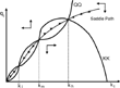
Proof. From above, we know that the QQ locus is always upward sloping. Since in this class of models there is a maximum sustainable capital stock, this implies that, for large k, the QQ locus will be above the KK locus in (kt, qt) space. Given this, the proposition follows from Figure 1 and Proposition 3. Figure 1 depicts the case in which there are multiple steady-state equilibria. Uniqueness and non-existence of nontrivial steady-state equilibria can be analyzed as special cases of Figure 1, where the origin is placed at the second and third steady states in Figure 1, respectively.

Global dynamics of an economy with land for the case in which there are three nontrivialsteady-state equilibria, whichare labelled $ \bar{k}_{l}$, $ \bar{k}_{m} $, and $ \bar{k}_{h} $; $ \bar{k}_{m} $ is an unstable steady state whereas $ \bar{k}_{l} $ and $ \bar{k}_{h} $ are stable. Economieswith an initial level of kin the interval (0, $ \bar{k}_{m}) $ will converge to the steady state $ \bar{k}_{l} $ whereas economies with an initial level of k intheinterval ($ \bar{k}_{m},\infty) $ will converge to the steady state $ \bar{k}_{h} $.
In addition to the QQ and KK loci, Figure 1 also depicts the unique saddle path connecting all nontrivial steady-state equilibria. This saddle path is the locus of the perfect-foresight competitive equilibrium level of q for each level of k. Since the saddle path is monotonic in (kt, qt) space, then for every level of k there is a unique level of q that lies on the saddle path, and so, the competitive equilibrium is unique. This is set out in Proposition 5.
PROPOSITION 5. Under Assumptions 1–3, for every level of k there is a unique level of q that satisfies the conditions of a competitive perfect-foresight equilibrium.
Proof. The global properties of the dynamical system are qualitatively the same as the two-sector model of Galor (1992). Consider first the case in which there is a unique nontrivial steady-state equilibrium. From above, we know that this nontrivial steady state will be a saddle point. From Corollary 1, Φ(kt, qt) is a diffeomorphism, and so, the stable manifold theorem4
See Guckenheimer and Holmes (1983 p. 18).
In the case of multiple nontrivial steady-state equilibria, we know from above that the stability of the nontrivial steady states will alternate between being unstable nodes and saddle- points. In this case the global stable manifold of each saddle-point stable steady state must lead to the unstable steady-states to the northeast and southwest of the saddle-point steady state. In this way the global stable manifolds of the saddle-point stable steady states connect all the steady-state equilibria and so do not overlap. Thus, for any initial level of the state variable kt, there will exist a unique value of qt such that the economy converges to a steady-state equilibrium.
Points that are not on a global stable manifold can be shown not to be consistent with perfect-foresight equilibria because their trajectories must lead to either a negative price of land or a value of land that is greater than the value of total output in the economy. Thus, the unique value of qt such that the economy converges to a steady-state equilibrium is the unique perfect-foresight competitive equilibrium.
Example of multiple steady-state equilibria
Figure 1 also depicts the case in which there are multiple nontrivial steady-state equilibria. Multiple steady-state equilibria can occur when there is a low elasticity of substitution between capital and other factors, as in Galor and Ryder (1989) or when there is nonhomothetic savings function; see Azariadis (1996). Appendix 2 gives an example of multiple steady-state equilibria in this model.
EFFECTS OF LAND TAXATION
In this section, we analyze the effects of land taxation in this model. We show that land taxation can cause a bifurcation in the dynamical system defined in the preceding section. Consequently, we can show how changes in the rate of land taxation can cause an economy with a low initial capital stock to break out of a low-income poverty trap steady-state equilibrium.
The intuition for these results is that since the productive input of land in the following period is unaffected by its price, and since any savings spent purchasing land are by definition not spent increasing next period's productive potential by being invested in capital, then a lower equilibrium price of land will ceteris paribus imply a higher level of production in the following period. Land taxation has the effect of reducing the price of land and hence has the effect of increasing capital accumulation. If there exist multiple steady-state equilibria, there will exist a threshold level of land taxation such that if the rate of land taxation is raised above this level then there will be a discrete upward jump in the steady-state level of income. This occurs because the increased level of capital accumulation eliminates the low-income steady-state equilibrium and causes the economy to converge to a higher-income steady-state equilibrium. Finally, given the result of McCallum (1987), we know that all steady-state equilibria in this economy are dynamically efficient and hence that the higher level of income implies a higher level of steady-state welfare.
We proceed by first deriving Lemma 1, which shows how a tax on the rents from land will cause the QQ locus to shift down. Lemma 2 then shows that the manner in which the tax revenue is spent by the government affects the KK locus. Since modeling the determination of government policy is not the subject of this paper,5
we simply present two polar extremes of government spending behavior. In one the government spends all tax revenues from land immediately on the final good so that cGt = τπt, where cGt is government spending on consumption in period t. In the other the government saves all tax revenues and consumes the proceeds from this investment in the following period, so that sGt = τπt and cGt = (1 + rt − δ)kGt, where sGt is the government's investment in the accumulation of capital in period t and kGt is the government's share of the capital stock due to its saving in the previous period. Lemma 3 proves that all steady-state equilibria are dynamically efficient. We then use Lemmas 1, 2, and 3 to derive our results, which are placed in Propositions 6 and 7 and Corollary 2.LEMMA 1. Under Assumptions 1 and 2, the imposition of a tax on the rents from land will cause the QQ locus to shift downward in
space.
Proof. Defining τ as the rate of tax on the rents from land, and then using equation (3), the QQ locus can be written as qt = πt+1(1 − τ)/(rt+1 − δ). Differentiating this expression directly with respect to τ and qt shows that ∂qt/∂τ < 0.
LEMMA 2. Under Assumptions 1 and 2, if the government spends tax revenue from land only on consumption, then the KK locus will be unchanged, but if the government spends tax revenue from land on capital accumulation, then the KK locus shifts upward.
Proof. If we define sGt as the government's per capita spending on capital accumulation then the equation for the KK locus becomes s(wt, rt+1) + sGt − qtm − kt = 0. Clearly, if sGt = 0, then the KK locus is the same as in Section 2.4.2, where there is no taxation of land. However, if sGt>0, then for a given level of k the level of qt must be higher for the equality to be maintained. Hence the KK locus shifts upward in (kt, qt) space.
PROPOSITION 6. Under Assumptions 1 and 2, the imposition of a tax on the rents from land can cause the dynamical system of the economy to change from one in which there exist multiple steady-state equilibria to one in which there is a unique nontrivial steady-state equilibrium.
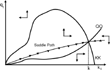
Proof. This follows from Lemma 1 and Figure 2. Figure 2 represents the case in which sGt = 0 but the result still clearly holds for the case in which sGt>0 and the KK locus shifts upward.

Effect of a high rate of taxation onearnings from land where a high rate of taxation on land revenues can change thedynamical system from having multiple steady-state equilibria tohaving a unique steady-state equilibrium. Thus, a high rate of landtaxation may break an economy out of a low—poverty trap—level of GDP per capita. In this case, alltax revenues are spent on consumption and the KK locus isunchanged, but the result clearly still holds for the case in whichthe KK locus shifts upward.
COROLLARY 2. Small changes to the rate of taxation on the rents from land can cause an economy with a low initial capital stock to break out of a low-income “poverty trap” steady-state equilibrium.
Proof. This follows from Proposition 6. When the system has multiple nontrivial steady-state equilibria, a low initial capital stock will imply that the economy will converge to a low-income-per-capita steady-state equilibrium such as
in Figure 1. However, if τ, the rate of tax on the rents from land, is sufficiently high, then as shown in Proposition 6 and Figure 2, the low-income-per-capita steady state disappears and the economy will converge toward a higher steady-state level of income per capita.
LEMMA 3. Under Assumptions 1 and 2, all steady-state equilibria are dynamically efficient [McCallum (1987)].
Proof. In this economy, using the analysis of Diamond (1965), the welfare of an agent at the steady state is maximized where fk = δ. However, from Section 2.4.1, it is seen that fk>δ in the steady state. Hence, there is always underaccumulation of capital relative to the maximum steady-state welfare level of k. This is a restatement of McCallum's (1987) result that the presence of productive land rules out dynamic inefficiency.
PROPOSITION 7. The welfare of agents at a steady-state equilibrium is increasing in the level of
.
Proof. This follows from Lemma 3 and Diamond's (1965) analysis that steady-state welfare will be increasing in the total resources available for consumption in the steady state. This is given by
, which given Lemma 3 is increasing in
.
CONCLUSION
This paper has analyzed the global dynamics of an intertemporal three-factor general equilibrium growth model. It has derived a unique perfect-foresight competitive equilibrium. It has shown that in this model, changes in the rate of land taxation may cause a bifurcation in the model's dynamical system and so may allow an economy with a low initial capital stock to break out of a “poverty trap” steady-state equilibrium.
APPENDIX
Proof that the Stability of a Steady State is Determined by the Relative Slopes of the KK and QQ Loci
The economy's dynamics are described by equation (4) in the text.
For ease of exposition we denote the Jacobian matrix of the economy at a steady state,
by J; that is,
. We also rewrite the Jacobian matrix of the economy at a steady state, J, as follows:

which defines the terms A ≡ swwk, B ≡ 1 + rt+1 − δ,
, and
LEMMA A.1. Under Assumptions 1 and 2, tr J>0, det J>0, and Δ ≡ tr J2 − 4 det J>0.
Proof. From Assumptions 1 and 2, tr J is the sum of two positive terms. After canceling terms, det J = AB/E, which is positive under Assumptions 1 and 2. Using this result, we can write

This can be rewritten as

which, from Assumptions 1 and 2, is always positive.
COROLLARY A.1. The eigenvalues of matrix J are real and distinct.
Proof. The eigenvalues of matrix J, λ1, λ2, are given by the formula λ1,2=[tr J ± √Δ]/2. Thus, from Lemma A.1, they are real and distinct.
LEMMA A.2. If tr J>0, det J>0, and Δ ≡ tr J2 − 4 det J>0, then under Assumptions 1 and 2, the eigenvalues of matrix J are both positive and
- λ1>1 if and only if either [tr J ≥ 2] or [1 − tr J + det J < 0]
- λ2>1 if and only if [tr J>2] and [1 − tr J + det J>0];
- 0 < λ2 < 1 if and only if either [tr J ≤ 2] or [1−tr J + det J < 0].
Proof. See Galor (1992, Lemma A1).
Given Lemmas A.1 and A.2, we can show that the stability of a steady state is determined by the relative slopes of the KK and QQ loci at the steady state. This is Proposition 3 in the text for which we provide the following proof.
Proof of Proposition 3. Given Lemmas A.1 and A.2, it is sufficient to show that when dq/dk|KK>dq/dk|QQ that [tr J>2] and [1 − tr J + det J>0] and that when dq/dk|QQ>dq/dk|KK that [1 − tr J + det J < 0].
We can rewrite [1−tr J+det J] as

which can, in turn, be rewritten as

According to our new notation, the slopes of the QQ and KK loci can be written as

Thus, we can write

and thus we have

Now, tr J = [(A/E) + B − (C − D)(m/E)]. From Assumptions 1 and 2, all three terms are positive. A positive steady-state level of q implies that rt+1 − δ>0, which implies that B>1. Also, since the QQ locus is always positively sloped, (dq/dk)|KK>(dq/dk)|QQ implies that the KK locus is positively sloped and hence that A>E and thus that A/E>1. Thus, tr J>2 when (dq/dk)|KK>(dq/dk)|QQ.
EXAMPLE OF MULTIPLE STEADY-STATE EQUILIBRIA
The simplest way of obtaining multiple steady-state equilibria is to use the properties of the CES family of production functions. If a production function based on the CES family is used, and if there is a low elasticity of substitution between capital and labor, then even with a constant-savings propensity out of income (loglinear preferences), multiple steady-state equilibria can be obtained; see Azariadis (1996) and Galor and Ryder (1989).
For example, consider the following constant-returns-to-scale production function:

If we assume that savings are half of income, then the KK locus in (kt, qt) space is simply

and if we assume that δ = 0, then the QQ locus in (kt, qt) space is simply

For parameter values A = 0.1, B = 10, m = 5, and ρ = −2, there are two stable steady states at k = 0.051 and k = 3.011 and an unstable steady state at k = 0.512.
This is a revised version of a paper presented at the Econometric Society's European Meetings 1999 in Santiago di Compostella and at Seminars at Essex, Manchester, Southampton, and Warwick Universities and Royal Holloway, University of London.
References
Azariadis C.
1996
The economics of poverty traps.
Journal of Economic Growth
1,
449–
486.Google Scholar
Deaton A. &
G. Laroque
2001
Housing, land prices and growth.
Journal of Economic Growth
6,
87–
105.Google Scholar
De La Croix D. &
P. Michel
2002
A Theory of Economic Growth.
Cambridge, UK:
Cambridge University Press.
Diamond P.
1965
National debt in a neoclassical growth model.
American Economic Review
55,
1126–
1150.Google Scholar
Eaton J.
1987
Dynamic specific-factors model of international trade.
Review of Economic Studies
54,
325–
338.Google Scholar
Galor O.
1992
A two sector overlapping generations model: A global characterization of the dynamical system.
Econometrica
60,
1351–
1386.Google Scholar
Galor O. &
O. Moav
2002
Natural selection and the origin of economic growth.
Quarterly Journal of Economics
117,
1133–
1192.Google Scholar
Galor O. &
H. Ryder
1989
Existence, uniqueness, and stability of equilibrium in an overlapping generations model with productive capital.
Journal of Economic Theory
49,
360–
375.Google Scholar
Galor O. &
D. Weil
2000
Population, technology and growth: From the Malthusian regime to the demographic transition.
American Economic Review
90,
806–
828.Google Scholar
Grossman G. &
E. Helpman
2002
Interest Groups and Trade Policy.
Princeton, NJ:
Princeton University Press.
Guckenheimer J. &
P. Holmes
1983
Nonlinear Oscillations, Dynamical Systems and Bifurcations of Vector Fields.
Springer-Verlag.
McCallum B.
1987
The optimal inflation rate in an overlapping generations economy with land.
In W.A. Barnett &
K.J. Singleton (eds.),
New Approaches in Monetary Economics,
pp. 325–
339.
Cambridge, UK:
Cambridge University Press.
Persson T. &
G. Tabellini
2001
Political Economics.
Cambridge, MA:
MIT Press.
Global dynamics of an economy with land for the case in which there are three nontrivialsteady-state equilibria, whichare labelled $ \bar{k}_{l}$, $ \bar{k}_{m} $, and $ \bar{k}_{h} $; $ \bar{k}_{m} $ is an unstable steady state whereas $ \bar{k}_{l} $ and $ \bar{k}_{h} $ are stable. Economieswith an initial level of kin the interval (0, $ \bar{k}_{m}) $ will converge to the steady state $ \bar{k}_{l} $ whereas economies with an initial level of k intheinterval ($ \bar{k}_{m},\infty) $ will converge to the steady state $ \bar{k}_{h} $.
Effect of a high rate of taxation onearnings from land where a high rate of taxation on land revenues can change thedynamical system from having multiple steady-state equilibria tohaving a unique steady-state equilibrium. Thus, a high rate of landtaxation may break an economy out of a low—poverty trap—level of GDP per capita. In this case, alltax revenues are spent on consumption and the KK locus isunchanged, but the result clearly still holds for the case in whichthe KK locus shifts upward.
 You have
Access
- 7
- Cited by