1. INTRODUCTION
The prediction of physical quantities governed by a dynamical process is of ongoing interest. Often, the dynamical process is known and the propagation of quantities can be well described by a system of differential equations. However, it is almost always impossible to precisely determine the initial state and the kinetic parameters. In addition, intrinsic stochastic perturbations may spoil precise predictions. The degree of knowledge of the process and the initial state can be expressed by explicitly introducing uncertainties to the system. Many methods for solving differential systems under uncertainties are already introduced. Monte Carlo sampling (Gilks et al., Reference Gilks, Richardson and Spiegelhalter1995) is able to consider white noise but leads to large computational effort. Polynomial chaos expansion (Ghanem & Spanos, Reference Ghanem and Spanos1991) is an efficient method for a moderate number of random numbers, but the method is not able to consider white noise.
In Kohler et al. (Reference Kohler, Müller and Wever2014, Reference Kohler, Marzouk, Müller and Wever2015), we have developed a new method for uncertainty quantification, which is based on the propagation of discrete risk levels. In this paper, we point out the practical relevance of this kind of approach. In Section 2 we summarize some physical and technical applications, where the threshold behavior is important. Section 3 describes the basic method, derived in Kohler et al. (Reference Kohler, Müller and Wever2014). The main part of the paper is concerned with water grids. The transport of risk levels for contaminants in water grids is presented in detail. In this paper, we describe not only the pure application but also some extensions of our method. In particular, the treatment of junctions in water grids is considered. Of even higher importance is the discussion of conservation properties for the algorithm. Here, a detailed analysis is shifted into Appendix A.
2. THRESHOLD VALUES AND RISK LEVELS IN PRACTICE
Many physical and technical systems change their physical behavior when passing a certain threshold value. The observer of the system might be interested only in the information with which the probability the system is under the threshold value, in the critical region around the value, or above the threshold. In the following, we want to list several technical systems where the threshold behavior is important or even dominant for the observer:
-
• Waste water systems are characterized by having large overflow chambers. Valves are controlled to minimize the overflow that is piped into a river. The uncertainty in the system is caused by the unknown consumption behavior and by the uncertainty in rain prognosis. The observer is mainly interested in whether the water level in the overflow chambers is uncritical, critical, or whether the water overflows.
-
• The next application concerns contamination of drinking water systems. This application is presented in detail in Section 4. Here, we discuss the propagation of arsenate in water pipes and also consider those part of the arsenate attached at the wall of the pipes. Contamination takes place also in the air, especially in large cities. For example, EU Guideline 2008/50/EG (http://www.umweltbundesamt.de/themen/luft/regelungenstrategien/luftreinhaltung-in-der-eu) fixes the limits for NO, NO2, SO2, CO, lead, and fine dust; the limit for fine dust has been 25 μg/m3 since 2010 and will be reduced to 20 μg/m3 in 2020. This contamination is mainly caused by automotives driven by diesel engines. The amount of contamination is observed by several sensors in a city. The contaminant disperses by diffusion and airflow. Often one is only interested in whether the contamination is acceptable, critical, or the limits are exceeded.
-
• A metal oxide semiconductor field-effect transistor (MOSFET) is often used as an electronic switching device. If the voltage at the gate terminal exceeds a given threshold, then the current line between the drain and the source terminal is conducting (see Bakshi & Godse, Reference Bakshi and Godse2007).
In addition, in physics itself thresholds play an important rule. For instance, materials change their state of aggregation if the temperature crosses some threshold value. In the following, we mention some of these effects.
-
• There is an upper critical bound for the temperature above which the components of a mixture are miscible (UCST). One example is hexane and nitrobenzene. Here, the UCST is 19°C. Above this temperature, the two substances are miscible in all proportions (see Atkins & de Paula, Reference Atkins and de Paula2006). The UCST of metals is beyond their melting temperature.
-
• One of the most important threshold values in physics is the melting point of a material, which is the temperature at which a solid material changes to the liquid phase (Atkins & Jones, Reference Atkins and Jones2008). This temperature is defined at a given pressure (often atmospheric pressure). The freezing point is defined for the inverse direction. For most substances, the two threshold temperatures are equal. The well-known melting of ice to water is 0°C at one atmosphere pressure.
-
• The Neel temperature is the temperature above which a ferromagnetic material becomes paramagnetic. At this temperature, the macroscopic magnetic ordering is destroyed by the thermal energy (see Kittel, Reference Kittel2005).
In the preceding text, we have mentioned some technical and physical applications where the threshold values are decisive in terms of limiting norms or physical values. Often, the observer is not interested in the state itself (which is of cause uncertain in a real system), but only in the probability to be lower or beyond this value. In the following, we present a method where exactly these probabilities are determined. As an application, we present the propagation of contaminants in water pipes.
3. CELLULAR PROBABILISTIC AUTOMATA (CPA)
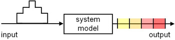
We (Kohlet et al., Reference Kohler, Müller and Wever2014) developed a CPA, which is time, space, and state discrete. Given an initial risk-level distribution, these levels are propagated by the CPA according to the system dynamics (see Fig. 1). Within this paper, we only summarize the main ideas of the algorithm.
Propagation of discrete system states under uncertainties. In practical applications, the model input is often uncertain and therefore represented as a probability density function. As output we are only interested in risk levels, modeled as medium to high probabilities (yellow to red) for discrete state space domains.

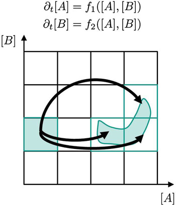
The method is used for a density-based uncertainty propagation of the dynamics of partial differential equations (PDE). The algorithm is designed as following: as described in Kohler et al. (Reference Kohler, Müller and Wever2014), the algorithm works in phase space. The discretization of the state leads to discrete boxes. The probability of the dynamical system to move from one box to the other is called the transition probability (see Fig. 2).
Discretized phase space of a two-dimensional dynamical system. The arrows indicate the transition probability, to propagate from one box to the other.

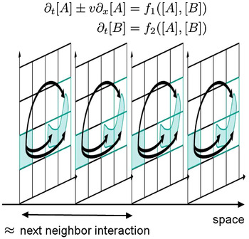
Phase state discretizations are known from ordinary differential equations, where they are used to describe limit cycles (see Dellnitz & Junge, Reference Dellnitz and Junge1999, Reference Dellnitz, Junge and Fiedler2002). In the context of the paper, we consider PDE. The additional complexity of space discretization is covered by assuming some locality conditions: only the nearest spatial neighbors are assumed to interact (see Fig. 3). We take into account that the interaction is identical at every node away from the boundaries. We can hence approximate the global transition distribution by a product of the same local transition distribution at every node. Such locality concepts belong to the core of cellular automata theory (Horlacher & Lüdecke, Reference Horlacher and Lüdecke2012; Ceccherini-Silberstein & Coornaert, Reference Ceccherini-Silberstein and Coornaert2010). The local transition probabilities can be specified as a conditional probability distribution.
The complexity of space discretization is reduced by considering only the interaction of the nearest neighbors.

The overall method is designed as a two-stage algorithm:
-
• In the first stage, all the transition probabilities of the discretized state are computed by using, for example, Monte Carlo computations. This first state, which can be regarded as a preprocessing step, is expensive in terms of computation time.
-
• In the second stage, the CPA can be evaluated for different initial conditions. This evaluation can be performed efficiently.
The consistency of the algorithm is proven by applying the Frobenius–Perron theory (Lasota & Macket, Reference Lasota and Mackey1993). The overall complexity of the algorithm is characterized by the number of boxes in the discretization of the phase space and the degree of locality for the space discretization (“pattern size”). The advantages of the algorithm may be summarized as follows:
-
1. As described in the Introduction, for many applications it is sufficient to propagate threshold behavior. Environmental threshold seems to be an especially important application. Our algorithm directly addresses this behavior.
-
2. The algorithm can be split into an expensive preprocessing part, which is the computation of transition probabilities, and an efficient evaluation part.
-
3. The results of the preprocessing part may also be used for solving inverse problems (see Kohler et al., Reference Kohler, Marzouk, Müller and Wever2015). No additional effort has to be invested for, for example, identifying parameters from measurements.
Sometimes the underlying PDE describes a conservation law. By adapting the local transition rule slightly, the CPA can be forced to preserve the expected value of the conserved quantity (see Fuks, 2013). The conservation properties of the algorithm, which are not covered by Kohler et al. (Reference Kohler, Müller and Wever2014, Reference Kohler, Marzouk, Müller and Wever2015), are discussed in Appendix A.
4. APPLICATION: WATER GRID
4.1. Risk assessment in water grids
Reliable drinking water supply in regulated quality is one of the most important privileges of a human population. A drinking water supply system is a controlled closed system, from water sources over pipelines, storage tanks, and meshed grids to end user. Nevertheless, there might be unmeant disturbances in quality, safety, and reliability that might cause threats for consumers, which have to be avoided by early detection and fast reaction.
Drinking water contamination can arise from different sources, for example, by operational incidents like equipment failure, operator mistakes, organizational faults, communications failure, road works, or fire suppression. However, cross-contamination by fatigue or corrosion as well as environmental events, such as heavy rain, biological growth, or raw water quality, could cause drinking water contamination. In addition, contamination can be caused intentionally by vandalism, sabotage, crime, and terrorism. There are strong ambitions in standardization and regulation of drinking water quality monitoring and control systems internationally in regard to not only drinking water sources and feedings but also drinking water supply to consumers inside of underground water distribution pipeline networks, especially since 9/11. Primary targets of a water safety plan (World Health Organization, 2008) are, among others,
-
• the understanding of the specific system regarding hazard assessment and risk characterization (critical sections to be observed),
-
• the identification of hazards and potential contamination with harmful outcome (injection localization and spread), and
-
• monitoring and verification of counter measures.
The Deutscher Verein des Gas- und Wasserfaches (DVGW) proposes a method for risk-based and process-oriented management for water operation in W1001 (Safety and security in drinking water supply; Niehues, Reference Niehues2010). Based on the description of the supply system, including infrastructure, flow diagram, and consumer profile, a hazard analysis and risk assessment can be done systematically and customized to support high safety, security, and reliability in the system and in measured derivation and verification for risk control.
Beside offline risk assessment for water grids, novel online early warning systems should support the event detection and hazard classification to distinguish between potential contamination incidents and normal operation. Usually monitoring of operational systems is done by installed sensors delivering online field data to be analyzed. However, actually it is too expensive to invest, install, and maintain enough chemical or biological sensors for water quality control applications inside the widespread undergrounded pipeline distribution network for drinking water. Model-based simulated information completion is necessary to get the area-wide and continuous picture of the system state and to forecast spread of potential contamination and hazard outcome as well as handling of countermeasures. In addition, US and European research shows that there are too many different possible contaminants in water for direct detection to be economically feasible. Only indirect indicators for contamination out of water quality parameters, such as conductivity, turbidity, or pH, can be monitored at selected points. The US Environmental Protection Agency (EPA) “Distribution System Water Quality Monitoring: Sensor Technology Evaluation Methodology and Results” (2009) provides a sensor guideline. Within the Threat Ensemble Vulnerability Assessment project under the management of EPA, the Sensor Placement Optimization Tool supports the optimal placing of water quality sensors in using EPANET-MSX for modeling complex reactions during transportation in water distribution systems and the contamination event detection software, CANARY, has been developed (EPA, 2007). The EU project SecurEau carried out within the EU seventh Framework Program research on “State of Art on Chemical Sensors for Early Warning Systems” (Monsorez, Reference Monsorez2009). It is expected that an early warning system will employ standard online water quality sensors to detect deviations, or anomalous events, from baselines.
The present paper introduces a model-based decision support system using the CPA method in case of contamination, for hazard and risk analysis as well as for countermeasure validation in water distribution networks. Combining the hydraulic model with the load transport inside of distribution networks, this method includes the uncertainty of concentration of contaminant pipe and of source localization.
4.2. Modeling approach
The simulation of contaminant fate in water grids is a multiphysics problem, where hydraulics and chemical kinetics have to be combined (Shang et al., Reference Shang, Uber, Rossman, Janke and Murray2011; Horlacher & Lüdecke, Reference Horlacher and Lüdecke2012). We decouple both phenomena and focus only on the chemical kinetics on the basis of a simplified water model. The simplified model is the result of a sophisticated hydraulic simulation with SIWA, a commercial software package from Siemens (Siemens AG, Reference Siemens2012). We use SIWA to model, illustrate, and simulate the hydraulics of a water grid defined by reservoirs, pumps, junctions, valves, pipes, consumers, and a given topology. We assume tubular pipes throughout the whole network. Only the water velocity in each pipe is extracted, which constitutes, together with length, radius, and topology of the pipes, the simplified model. The chemical kinetics can then be described by advection–reaction equations for pipe dynamics and algebraic couplings for conservation at junctions. In practice, this simplification might be enough, when we only consider risk levels anyway.
Concentrations of dissolved species are usually given in units of mass per water volume, while species at the pipe walls are described in units of mass per wall area. The interaction of both types can be described with the help of the quotient of the cross-sectional pipe area and the wetted perimeter of the cross section, the hydraulic radius r h. For tubular pipes, the hydraulic radius is just half of the usual radius r, r h = (r/2). The chemical kinetics thus differs with the radius of the pipe in which it takes place. When describing the chemical kinetics with CPA, in principle, the preprocessing has to be conducted for every pipe radius in the grid. However, as pipes are usually standardized, only a few preprocessing runs are necessary in practice.
Besides the radius, there is one more parameter that may vary from pipe to pipe in the simplified advection–reaction model: water velocity. However, different water velocities do not require several CPA preprocessings. We use a global time step for all pipes and calculate an individual space step according to a pipe's velocity. By adjusting the number of sites per pipe to the length and space step of the pipe, we can therefore approximately use the same CPA for all different velocities.
4.3. Arsenate in water pipe
The advection and adsorption of arsenate in drinking water pipes is already considered in Kohler et al. (Reference Kohler, Marzouk, Müller and Wever2015). The physics is described by the Langmuir adsorption model (Koopal & Avena, Reference Koopal and Avena2001). Here, we only briefly present the basic physical equations:
 $$\eqalign{\partial_t D + v \partial_x D &= - {1 \over r_{\rm h}} f\lpar {D\comma\, A} \rpar\comma \cr \partial_t A &= f\lpar {D \comma\, A} \rpar\comma}$$
with
 $$f\lpar {D \comma\, A} \rpar = \displaystyle{1 \over \displaystyle{1 \over k_1} + \displaystyle{1 \over {k_f}} \lpar {S_{{\rm max}} - A} \rpar}\lpar {D\lpar {S_{{\rm max}} - A} \rpar - K_{{\rm eq}} A} \rpar \comma $$
where D is the concentration of dissolved arsenate and A the concentration of arsenate adsorbed at the pipe wall. The parameter values are taken from Klostermann et al. (Reference Klostermann, Murray, Szabo, Hall and Uber2010) and Pierce and Moore (Reference Pierce and Moore1982).
 $$\eqalign{v &= 10\displaystyle{\hbox{m} \over \min}\comma \quad r_{\rm h} = 50 \displaystyle{{\rm l} \over {\hbox{m}^2}}\comma \cr k_1 &= 0.2\displaystyle{{\rm l} \over \hbox{mg}\, \min}\comma \quad S_{\max} = 100\displaystyle{\hbox{mg} \over \hbox{m}^2}\comma \cr K_{\rm eq} &= 0.0537 \displaystyle{\hbox{mg} \over {\rm l}}\comma \quad k_f = 2.4 \displaystyle{{\rm l} \over \hbox{m}^2 \min}.}$$
For discretization, the advection and the reaction step are decoupled (see Thirring, Reference Thirring1981). For the advection, the method of characteristics (LeVeque, Reference LeVeque1999) is used with U = {−1, 0} as the backward difference, Δx = 100 m and Δt = Δx/v = 10 min:
 $$\eqalign{D^{n + 1}_i &= D_{i - 1}^n - \Delta t \displaystyle {1 \over r_{\rm h}} f\lpar {D_{i - 1}^n \comma\,\, A_i^n} \rpar \comma \cr A_i^{n + 1} &= A_i^n + \Delta tf \lpar {D_{i - 1}^n\comma\,\, A_i^n}\rpar.}$$
The total arsenate concentration D + [(1/r h)A] is a conserved quantity. Therefore, the transition probabilities undergo a slight adaptation proposed in Appendix A in order to preserve the expected value of the total arsenate concentration. A detailed analysis of conservation properties is given in Appendix A.
4.4. State-discrete modeling of junctions
To simulate whole water grids we extend the CPA algorithm to junctions. In this section, we introduce an algorithm for advection–reaction problems for an example with three pipes. For notational simplicity, we derive our idea just for a single dissolved species, but generalizations are straightforward. More complex applications are presented as part of the grid simulation in the next section.
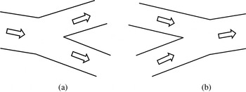
We note that due to the way we introduced time and space discretization, mixing is a local phenomenon. We only have to define a new local update rule for the first site of each output pipe. In principle we have to distinguish between two dynamically different types of junctions (see Fig. 4). If the flow direction is such that there is just one input pipe (Fig. 4a), concentrations can be handled easily. We do not have to think of any mixing for concentrations, as both water volume and species’ mass are split. Therefore, we can just apply the regular CPA rule on the neighborhoods consisting of the last site of the input pipe and the first site of each output pipe, respectively.
Two types of junctions have to be distinguished for cellular probabilistic automata simulation of an advection–reaction problem. In type (a) the hydraulics is such that we have only one inflow pipe that splits up, and in type (b) we have several mixing inflows.

We focus on the second case (Fig. 4b), where there are two input pipes a and b and one output pipe c. Here, the volume of water V i , water velocity u i , cross-sectional area A i , mass of dissolved species M i , and concentration of dissolved species D i denote the respective variables at the last site in pipe i ∈ {a, b} and at the first site of pipe i = c. The conservation of the species’ mass and the conservation of volume of the incompressible water read
 $$\eqalign{{M_c} &= M_a + M_b\comma \cr V_c &= V_a + V_{b}\comma}$$
and can be used to derive an equation for the concentration of the dissolved species in pipe c. We consider only the one-dimensional phase space
 $\tilde{\rm \Omega}$
of the dissolved species with partition
 $\lcub \tilde{\rm \Omega}_e \rcub _{e \in \tilde {E}}$
. Although
 $\tilde{\rm \Omega}$
and
 $\tilde{E} $
are the same at every site, we will attach indices a, b, c to them to clarify to which site we refer. Then
 $m: \tilde{\rm \Omega}_{a} \times \tilde{\rm \Omega}_b \times \tilde{\rm \Omega}_c$
is given by
 $$\eqalign{D_c &= m\lpar {D_a \comma\, D_b} \rpar = \displaystyle{{M_c} \over {V_c}} = \displaystyle{{M_a + M_b} \over {V_a + V_b}} = \displaystyle{{V_a D_a + V_b D_b} \over {V_a + V_b}}\comma\cr & = \displaystyle{{A_a u_a} \over \underbrace{A_a u_a + A_b u_b}_{\rm \alpha}}D_a+ \displaystyle{{A_b u_b} \over \underbrace {A_a u_a + A_b u_b}_{\rm \beta}} D_b\comma}$$
and has to be translated into discrete phase space. All we can get is again a probability distribution
 $m_0 : \tilde{E}_a \times \tilde{E}_b \to D\lpar \tilde{E}_c \rpar$
given by
 $$m_0\left( {e_a \comma\; e_b} \right)\left( {e_c} \right) = \displaystyle{{{\rm \lambda }\left( {{\rm \Omega }_{e_a} \times {\rm \Omega }_{e_b} \cap {\rm m}^{ - 1}\left( {{\rm \Omega }_{e_c}} \right)} \right)} \over {{\rm \lambda }\left( {{\rm \Omega }_{e_a} \times {\rm \Omega }_{e_b}} \right)}}.$$
If the partition
 $\{\tilde{\rm \Omega}_e \}_{e \in E}$
is uniform with resolution
 $\Delta \tilde{\rm \Omega}$
, then
 $m \lpar \tilde{\rm \Omega}_{e_a}\comma\, \tilde{\rm \Omega}_{e_b} \rpar $
is also an interval of length
 $\Delta \tilde{\rm \Omega}$
for all e
a
, e
b
∈ E: Let
 $\tilde{\rm \Omega}_{e_i} = \lsqb {v_i\comma\, w_i} \rsqb $
for i ∈ {a, b}, and denote m([v
a
, w
a
], [v
b
, w
b
]) = [v
c
, w
c
]. Note that by definition α, β ≥ 0 and α + β = 1. Therefore, v
c
= αv
a
+ βv
b
and w
c
= αw
a
+ βw
b
, and so
 $$w_c - v_c = {\rm \alpha }\left( {w_a - v_a} \right) + {\rm \beta }\left( {w_b - v_b} \right) = \left( {{\rm \alpha } + {\rm \beta }} \right)\Delta \tilde{\rm \Omega} = {\rm \Delta} \tilde{\rm \Omega}.$$
Similar to the extension discussed in Appendix A, m 0 might also be adapted to include conservation considerations. Furthermore, m 0 has to be embedded in the n-dimensional phase space Ω of dissolved and adsorbed species to get the whole mixing rule.
4.5. An exemplary municipal grid
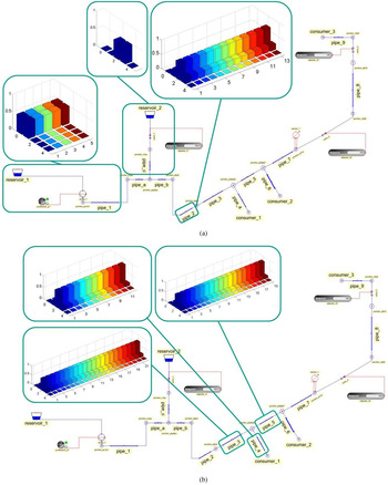
We apply our ideas to a part of a municipal drinking water grid given in Figure 5. It consists of many elements, of which we extract for CPA simulation nine long pipes, three consumers, and two sources, the reservoirs. The rest of the elements is just needed for the hydraulic simulation: Reservoir 2 is attached to Pipes 1 and 2 by very short connection Pipes a, b, and c. However, they are so short that their influence on chemical kinetics can be neglected. Pumps and elevation parameters for all objects establish a pressure profile that leads to water flow to the consumers. Some valves can be used to control the hydraulics.
The topology of a part of an exemplary municipal grid. The grid mainly consists of nine long and three short pipes, two reservoirs, and three consumers. For the hydraulic simulation with SIWA the pumps and valves are also necessary, which can in principle be controlled online with the red boxes. The steady state after 4 days is shown for the dissolved arsenate and both junction types, in (a) for Reservoir 2 and Pipes 1 and 3, and in (b) for Pipes 3, 4 and 5. In each diagram the vertical axis depicts the probability of being in the domain 0 to 4 at the respective site.

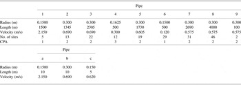
For simplicity, all setup parameters such as demand and pump profiles are assumed to be constant in time such that the system is in a hydraulic steady state. A SIWA simulation in a realistic exemplary setting leads to the following parameters for a simplified advection–reaction model as shown in Table 1.
The parameters for a simplified advection-reaction mode

We describe advection and adsorption of arsenate in the grid like in Section 4.3 with the model of Eq. (1). The chemical parameters are given in Eq. (2), but the hydraulic and the pipe parameters are, of course, different. We consider the system on the approximately positively invariant state space domain given by
 $D \in \lsqb {0\comma\; 1} \rsqb \hbox{mg}/\hbox{l}$
and
 $A \in \lsqb 0\comma \; 100 \rsqb \hbox{mg}/\hbox{m}^2 $
. The translation to CPA with the postprocessing covered in Appendix A is conducted three times according to the three different pipe radii (see Table 1 and the discussion in Section 4.2). To discretize time and space, we decouple again the advection and the reaction step with the Trotter formula. For the advection, the method of characteristics is used with U = {−1, 0} as the backward difference and the global time step Δt = 2.5 min. We map 75 × 37 randomly distributed test points by using intermediate steps with the less coarse discretization Δt′ = 0.1 min. The pattern length is minimal,
 $V = \tilde{V} = \lcub 0 \rcub $
, and the phase space partition equidistant with 5 domains in the D- and 15 in the A-direction.
In the CPA simulation, we choose the threshold probability .005. To describe the mixing in the formalism of Section 4.4, we model Reservoir 2 as a pipe with one site, the boundary condition, with the characteristics of Pipe c. The number of sites in each pipe is calculated by dividing the length by the global time step and the velocity. The inflow boundary conditions of Pipes 3, 8 and 9 are just the last sites of the previous Pipes 2, 7 and 8, respectively. At the inflow of Pipes 4, 5, 6 and 7, the trivial mixing rule is applied, and at the inflow of Pipe 2, the nontrivial.
We want to simulate the spread of arsenate in Reservoir 2 through the network over time, while the rest of the grid, in particular Reservoir 1, is not contaminated in the beginning. As initial conditions, we thus choose the lowest state with probability 1 for dissolved and adsorbed arsenate throughout the whole network, except for Reservoir 2. In Reservoir 1 the boundary condition for the dissolved arsenate is the lowest state with probability 1, and in Reservoir 2, a distribution over higher states (see Fig. 5a). Because of the Trotter discretization, we do not have to specify a boundary condition for the adsorbed arsenate.
The time evolution is simulated over 4 days, and it can be displayed at every site. We only show as an exemplary result in Figure 5 the final steady state for dissolved arsenate in the pipes involved in mixing. In the steady state, the adsorbed arsenate is everywhere in the grid approximately in State 13 with probability 1. An exception is, of course, Pipe 1 (see behavior in last Appendix A figure). The simulation time is with about 6 h on a common laptop, much shorter than the simulated time. The preprocessing time was approximately 3 times 1.25 h. As the algorithm is rather straight to parallel, it is possible to speed up the simulation on suited computer clusters.
The algorithm developed in Kohler et al. (Reference Kohler, Müller and Wever2014) does not guarantee the conservation of physical quantities. Nevertheless, this is an important property for the propagation of fate contaminants in water grids. Because of the more mathematical nature of the derivation, we shift this part to discussion in Appendix A.
We are able to simulate under uncertainties a large grid faster than real-time by calculating directly on a simplified state space. The state space allows for a direct practical interpretation in terms of contamination risk levels. Our example comprises the features introduced in the former sections: the unexpected accumulation of probability in State 3 for the dissolved arsenate due to the nonlinearity of the interaction, the mass conservation, and the mixing behavior. Already in this simple setup we gather interesting information for the consumer that would not be available in a deterministic simulation. In chemically and topologically more involved examples, we expect the consumer to really benefit from results that cannot be simulated easily by other means.
5. CONCLUSION AND OUTLOOK
In this paper, we have presented a characterization and a detailed application for the algorithms developed in Kohler et al. (Reference Kohler, Müller and Wever2014). In Appendix A, we present ideas on how to extend the algorithm for conserving physical quantities. Our ideas work for hydraulic steady states on which we have focused in this work. With the concepts of inverse engineering presented in Kohler et al. (Reference Kohler, Müller and Wever2015), the application can be easily extended for detecting leaks in the water pipes.
The efficiency of the method strongly depends on the dimension of the phase space. Applications such a chemical reactions, which are described by a huge number of equations, are less suitable for the method. However, conservation laws, such as the Euler equations of the Navier–Stokes equations, seem to be a promising application. Further work is needed to extend the method to these equations.
APPENDIX A
A.1. Conservation laws in CPA
Here, we intend to investigate the CPA with respect to conservation laws. These considerations are motivated by the arsenate application, for which we expect conservation of the total arsenate. In the Section A.1 we show an example in which the CPA method violates the conservation law. In Section A.2, we suggest an extension of the regular CPA method to impose conservation. Finally, in Section A.3, the method is applied to solve the problem in the arsenate example.
A.2. Violation of conservation in CPA
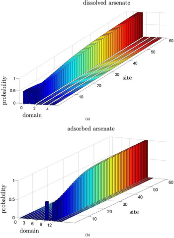
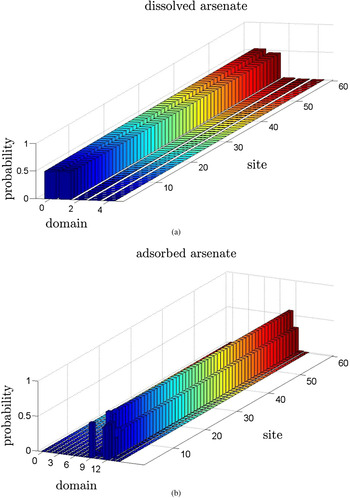
Reconsider the transport and advection of arsenate of Section 4.3, which means the system of Eq. (1) with the parameters of Eq. (2). We apply the Trotter formula and the method of characteristics to the differential equations (3), and choose the same space and time steps. The state space is discretized in 5 domains in the D-direction and in 15 domains in the A-direction. The only difference from Section 4.3 is that we simulate a longer pipe with 60 sites now, and we impose the following stochastic boundary condition:
 $$g_l \lpar e \rpar = \left\{ \matrix{0.5 \hfill &{\rm if} e = \lpar {0 \comma 9} \rpar \hfill \cr 0.5 \hfill &{\rm if} e = \lpar {1 \comma 13} \rpar \hfill \cr 0 \hfill &{\rm else} \hfill} \right.\comma$$
where the first symbol is the D-domain and the second the A-domain. The steady-state result after 4 days has been calculated with probability threshold 0.0001 and is shown in Figure A.1.
Simulation of arsenate transportation and adsorption in a long pipe with a regular local function: (a) the dissolved arsenate and (b) the adsorbed arsenate in the steady state. The total arsenate concentration is not conserved due to numerical errors.

In both the adsorbed and the dissolved arsenate direction, the probabilitiy accumulates in two neighboring domains throughout the whole pipe. We observe that for the respective domain with lower concentration, the probability at the entrance of the pipe is higher than the corresponding probability at the end of the pipe. In contrast, for the respective domain with higher concentration, the probability at the inflow is smaller than that at the outflow. This means that in the steady state, on average, the total arsenate inflow is higher than the outflow. However, the PDE model respects the conservation of total arsenate concentration. We find the hyperbolic conservation law
 $${\partial}_t \left( {D + \displaystyle{1 \over {r_{\rm h}}} A} \right) + v\,{\partial}_x D = 0 \comma$$
where the conserved quantity is the total concentration
 $$D + \displaystyle{1 \over {r_{\rm h}}}A\comma$$
and where the flow only consists of dissolved arsenate. Therefore, the conservation law is violated in the pipe. We will investigate that more formally in the next section.
We recap that uncertainty propagation with CPA consists of two steps, the preprocessing and the simulation. It is in the preprocessing, where the transition probabilities are determined to translate the PDE into a CPA, whereas the simulation step is completely independent of the PDE. We conclude that the violation of conservation is a matter of the preprocessing, and the errors from the preprocessing then accumulate in the simulation. Our approach is therefore to adapt the preprocessing to conservation laws.
A.3. Imposing conservation in the preprocessing
In this section, we suggest a method to adapt the CPA transition probabilities to conservation laws, that is, a postprocessing of the preprocessing before the simulation. There are various possible definitions of conservation in a probabilistic setting. We show that the expectation value of a conserved quantity is preserved during time evolution of a probability density, if it is preserved by the trajectories of all realizations. Therefore, we require our extension of the CPA preprocessing to assure that the expected values of the conserved quantities are preserved. We expect that the method can be extended to higher moments.
Formally, we consider the time- and space-discrete dynamical system with the locality property described in Section 3. We assume that the dynamical system is derived from a PDE by time and space discretization, and that a conservation law holds locally. In the following lemma,
 $V_{i + U}^n $
denotes the random variable that is the natural restriction of the random variable V
n
: X → Ω
m
to the (i + U)-coordinates of the image, where
 $i \in \tilde{I} $
. E[V] is the expected value of a real-valued random variable V (see Section 3).
Lemma: Let n ∈ ℕ0,
 $i \in \tilde{I} $
, measurable k : Ω
U
→ ℝ and k′ : Ω → ℝ such that
 $$k^{\prime}\lpar {v_i^{n + 1}} \rpar = k\lpar {v_{i + U}^n} \rpar $$
is fulfilled for every v n , v n+1 = Φτ(v n ) ∈ Ω m . Consider random variables V n , V n+1 = Φτ(V n ) : X → Ω m with densities g n , g n+1 = P Φτ (g n ) ∈ D(ℝ mn ), respectively. Assume that Φτ is injective and continuously differentiable. Then
 $$ E\lsqb {k^{\prime}\lpar {V_i^{n + 1}} \rpar } \rsqb = E\lsqb {k\lpar {V_{i + U}^n} \rpar } \rsqb.$$
■
Proof: It is well known (Lasota & Mackey, Reference Lasota and Mackey1993) that under the given assumptions g n+1(v) = P Φτ (g n )(v) = g n (Φ−τ(v))|detD(Φ−τ)|, where detD(Φ−τ) is the determinant of the Jacobian matrix of Φ−τ. Therefore,
 $$\eqalign{E\lsqb k^{\prime}\lpar V_i^{n + 1} \rpar \rsqb &=\int k^{\prime}\lpar {v_i} \rpar g^{n + 1} \lpar v \rpar dv \cr&=\int k^{\prime}\lpar {v_i} \rpar (g^n \lpar {\rm \Phi}^{-{\rm \tau}} \lpar v \rpar \rpar \vert {\rm detD}\lpar {\rm \Phi}^{-{\rm \tau}} \rpar \vert dv\comma \cr &=\int k^{\prime}\lpar{\rm \Phi}^{\rm \tau} \lpar {w \rpar_{i}} \rpar g^n \lpar w \rpar dw \cr&=\int k\lpar {w_{i + U}} \rpar g^n \lpar w \rpar dw = E\lsqb {k\lpar {V_{i + U}^n}} \rpar \rsqb\comma}$$
by substitution w = Φ−τ(v) and locality of Φτ. ■
Note that g n and g n+1 may be replaced by suitable marginal distributions when calculating the expected values of the local variables. Since a conservation law holds locally, the locality approximation in the CPA construction cannot be the cause of its violation. There remain just two steps in the translation from PDE to CPA, where things can go wrong: the numerical approximation of the Frobenius–Perron operator by test point mapping, and the subsequent restriction of image densities to the subspace of piecewise constant densities.
We suggest an algorithm that corrects the errors originating from both steps with respect to the expected values of the conserved quantities. The idea is to constrain the set of local functions to those that give rise to the exact expected values in the image distribution. Note that we know the exact expected value according to the above lemma. The transition probabilities are then chosen by an optimization such that they are as close as possible to the approximate image point distribution from the regular preprocessing.
We state the algorithm for notational simplicity only for one conserved quantity. It is straightforward to extend it to several of them by adding more constraints. For a given partition E of Ω and for all φ ∈ E U , we conduct the following steps:
-
Step 1. Determine vector m = (m e ) e∈E by m e = E[k′(V)], where V : X → Ω has uniform distribution over Ω e .
-
Step 2. Determine vector of nonzero preliminary transition probabilities p′ from φ to e ∈ E by mapping of test points with standard preprocessing.
-
Step 3. Determine for all image domains Ω e with nonzero probability the mean
 $\tilde{M} _e $
of the conserved quantity k′ with respect to the image points that it contains.
-
Step 4. Determine exact expected value M = E[k(V)] of the conserved quantity, where V : X → Ω U has uniform distribution over Ωφ.
-
Step 5. Determine a diagonal weight matrix W with diagonal elements (1/d e ), where
$d_e = \vert {m_e - \tilde{M}_e} \vert $
. -
Step 6. Solve quadratic program for new nonro transition probabilities p


 $$\eqalign {& (\,p - p^{\prime})^T W\lpar {\,p - p^{\prime}} \rpar \to \hbox{min\comma} \cr & M = {m^T p\comma \quad\!\! \parallel \!p \!\parallel_1 = 1\comma \quad p \ge 0\comma}}$$
where m just contains only the indices e ∈ E of the vector that appear in p′.
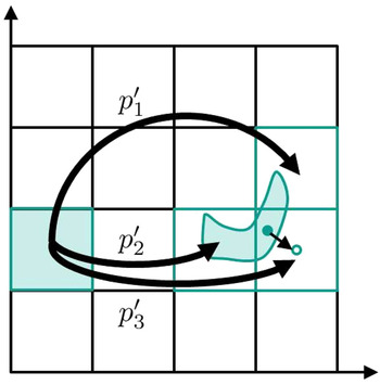
Figure A.2 gives some sense of what the algorithm does. We add five comments on the algorithm. First, we note that Step 1 is independent of φ, so it has to be computed only once. Second, the effect of the weight matrix W constructed in Steps 4 and 5 is to better maintain the approximate p′ when restricting the image density to be piecewise constant. The better the expected value of the conserved quantity with respect to the image points in one domain already matches the domain's expected value, the more expensive it is to change the probability in the optimization Step 6. A simple variant of the algorithm is of course to omit Steps 4 and 5 and choose W as the identity matrix in Step 6. Then the quadratic program turns into a least-squares problem. Third, we note that by only redistributing the probabilities for the domains with nonzero probability, we prevent the optimization from allocating nonzero probabilities to domains that are actually not in the support of the image density. However, for some φ ∈ E U , there might be no feasible solution to the quadratic program, because then the constraints for normalization and expected value are too strict. This happens especially for boundary domains. A practical workaround is to also include the neighboring domains in the optimization procedure. If we then still do not find any feasible solution, we keep the probabilities from the regular preprocessing. Fourth, we mention that there are other options to define the optimization problem, for example, by including the constraint for the expected value with a big constant in the minimization procedure. This would also help to find feasible solutions more frequently. Fifth, we note that the additional computational effort of the postprocessing is negligible in practice. We only have to execute one optimization for every preimage pattern, which is much less expensive than the test point mapping.
We show one site with an exemplary two-dimensional phase space partitioned in 16 boxes to illustrate the postprocessing. The preimage state at this site is the left green box, and the standard preprocessing assigns in this example probabilities p ′1, p ′2 and p ′3 to thr image domains (boxes with green boundaries). All domains that have an intersection with the images of the test points (green shape) are considered as image domains. The exact conserved expected value M is calculated from the preimage state. In one of the image boxes, we exemplary sketch M̃e . by a filled green circle and m e by a green circle with white interior. The quadratic program redistributes the probabilities according to the differences in M̃e and m e such that the expected value is conserved exactly.

A.4. Application: Adsorption of arsenate
In the arsenate application, the conserved quantity is the total arsenate concentration. With the time and space discretization of Eq. (3), we find that
 $$D_i^{n + 1} + \displaystyle{1 \over {r_{\rm h}}} A_i^{n + 1} = D_{i - 1}^n + \displaystyle{1 \over {r_{\rm h}}} A_i^n.$$
Therefore, we can identify
 $$k\lpar {v_{i + U}^n} \rpar = D_{i - 1}^n + \displaystyle{1 \over {r_{\rm h}}} A_i^n\comma \quad k^{\prime}\lpar {v_i^{n + 1}} \rpar = D_i^{n + 1} + \displaystyle{1 \over {r_{\rm h}}} A_i^{n + 1}.$$
When we conduct an extended preprocessing with the parameters of Section A.1, we include also the next neighbors in the optimization. As a result, we find a feasible solution for all preimage states, and the new transition probabilities differ slightly from the regular preprocessing. A remarkable difference is that now whereas without the postprocessing we had f 0(0, 0)(0) = 0.9446 and f 0(0, 0)(1) = 0.0554. With the extended preprocessing, it is not any longer possible by numerical mistakes that arsenate is created in an empty pipe.
With the new local function, we repeat the same simulation as in Section A.1. The results for the steady state after 4 days are shown in Figure A.3. Even in a long pipe, we can now guarantee conservation of the expected value of the total arsenate concentration. The unphysical numerical phenomenon described in Section A.1 no longer appears. Furthermore, simulations in the setup of Section 4.3 with the new local function show very similar results to the old local function. Especially the accumulation of dissolved arsenate in risk level 3 can still be observed (see Figure 5 for an example with similar parameters). We note that in practice it is critical to choose the threshold probability in the simulation for considering a probability to be nonzero quite low, so that small errors cannot accumulate. Here we used 0.0001.
Simulation of arsenate transportation and adsorption in a long pipe with an improved local function: (a) the dissolved arsenate and (b) the adsorbed arsenate in the steady state. In contrast to Figure A.1, now the expected value of the total arsenate concentration is conserved.

Dominic Kohler works in the Energy Management Department at Siemens in Erlangen, Germany, where he focuses on strategic questions in energy grids. Dominic’s first touchpoint with infrastructure questions was his PhD thesis on simulation of water grids under uncertainty, which he completed in a collaboration between the Department of Mathematics at the Technical University of Munich and the Corporate Technology Department of Siemens in Munich. Dominic’s mathematical interest lies in applications of advanced analytics to industrial problems, especially in uncertainty quantification, inverse problems, partial differential equations, and cellular automata.
Johannes Müller is a Professor in the Department of Mathematics at the Technical University of Munich. He was previously a Group Leader at the Institute of Biomathematics and Biometry at Helmholtz Zentrum München and an Interim Professor in Cologne. Johannes completed his undergraduate studies at the University of Karlsruhe and received his PhD and Lecturer Qualification at the University of Tübingen. Prof. Dr. Müller’s research explores the interface between mathematics and life sciences. He is particularly interested in the use and further development of dynamic systems and stochastic processes, as required by modern methods in biology and medicine.
Birgit Obst is Senior Key Expert Engineer in the Corporate Technology Department of Siemens in Munich. Birgit received her diploma in mathematics at the Technical University of Munich. Since 2001 she has worked in modeling and simulation technologies of plants and technical systems at Corporate Technology, Siemens. Her main interest lies in simulation architecture and model based applications for operational decision support and optimized strategies in condition monitoring and plant management.
Utz Wever is a Mathematician in the Corporate Technology Department of Siemens in Munich and holds a lectureship at the Technical University of Munich. Utz completed his undergraduate studies at the University of Munich and received his PhD at the University of Kaiserslautern and University of Munich. His current mathematical interests are in uncertainty quantification and model order reduction of dynamical systems. Dr. Wever’s field of applications ranges from semiconductor simulation, thermoacoustic stability evaluations for gas turbines, to simulative operation support for large systems.