



1. Introduction
The famous Khintchine theorem (see Theorem 1 in Subsection 2 below) was established more than a century ago and is now regarded as one of the central results in the metric theory of Diophantine approximation. It states that, for almost all real numbers, the precision of their best rational approximations is asymptotically essentially the same. In 1964, Schmidt [Reference Schmidt18] refined this theorem by showing that, for almost all real numbers, the best rational approximations appear at fairly regular intervals. Both of these results rely on the assumption that the approximating function ψ is monotonically non-increasing. The Duffin–Schaeffer conjecture, which allows for non-monotonic ψ, remained open for nearly eight decades and was ultimately proved by Koukoulopoulos and Maynard in 2021 [Reference Koukoulopoulos and Maynard11]. The corresponding Schmidt-type refinement appeared even more recently, in 2022, by Aistleitner, Borda, and Hauke [Reference Aistleitner, Borda and Hauke1]. These latter two results concern the homogeneous case, whereas the inhomogeneous Duffin–Schaeffer conjecture remains unresolved.
A natural extension of these theorems involves restricting the set of possible denominators rather than allowing all integers; see, for example, [Reference Pollington, Velani, Zafeiropoulos and Zorin15]. Early work in this vein focused on rapidly growing (lacunary) denominator sequences qn. Subsequent efforts aimed to slow down the growth of qn. To the best of our knowledge, this is the first article to establish inhomogeneous results for polynomially growing sequences qn.
Our main result, Theorem 3, gives an asymptotic relationship as in Schmidt’s theorem, or also in Aistleitner-Borda-Hauke theorem, for approximations with restrained denominators, and this is a metric result applicable to a wide class of measure spaces, rather than only to Lebesgue’s measure. The motivation for this expansion is explained further in this section. Our result does not need the assumption of the monotonicity of the function ψ and treats general inhomogeneous situations, as well as homogeneous ones. So it could be seen as a strong asymptotic version of the inhomogeneous Duffin–Schaeffer conjecture with restrained denominators on M 0-sets.
This paper develops further the metric theory of Diophantine approximations on so-called M 0-sets.
Definition 1. The set F is called an M 0-set if it supports a non-atomic probability Borel measure  ${\mu}$ (
 $\text{supp}(\mu) \subset F$) whose Fourier transform
 $\widehat{\mu}$ vanishes at infinity, i.e.
 \begin{align*}\lim_{|t| \to \infty} |\widehat{\mu}(t)| = 0,\end{align*}
where
 \begin{align*} \widehat{\mu}(t) \, := \int e^{-2\pi it x} \, \mathrm{d}\mu (x), t\in \mathbb{Z}.
\end{align*}
Such a measure  ${\mu}$ is called a Rajchman measure.
The interest in studying M 0-sets is bifold. On the one hand, there are quite many classical (fractal) sets of interest that support a Rajchman measure (see, for example, [Reference Bluhm3, Reference Bluhm4, Reference Hambrook7, Reference Kaufman9, Reference Li and Sahlsten12, Reference Queffélec and Ramaré16]). On another hand, it is quite natural to expect, at least heuristically, that such measures’ behaviour have significant similarities with Lebesgue measure: indeed, one would naturally expect that, as  $|\hat{\mu}(t)|$ tends to 0 as
 $t\to\infty$, the behaviour of
 ${\mu}$ is determined to a significant degree (whatever it means in concrete terms) by some first coefficients,
 $\hat{\mu}(t)$ for
 $t=-N,\dots,N$. And then, of course, the measure with Fourier transform
 $\sum_{t=-N}^N\hat{\mu}(t)\exp\left(-2\pi i t x\right)$ is absolutely continuous with respect to Lebesgue (Indeed,
 $Q(x):=\sum_{t=-N}^N\hat{\mu}(t)\exp\left(-2\pi i t x\right)$ is a trigonometric polynomial. So it is preserved by both the Fourier and inverse Fourier transforms. Consequently, if we consider the measure ν on
 $[0,1]$ with density defined by Q(x), its Fourier transform is given by Q(x) (and by uniqueness of Fourier transform, this is the only measure with this given Fourier transform). At the same time, ν is clearly absolutely continuous with respect to Lebesgue measure (we explicitly have its density)). See a more detailed discussion and some further references in [Reference Pollington, Velani, Zafeiropoulos and Zorin15], where some quantitative results that illustrate the heuristics above have been proven and some other results from the past literature have been discussed from this point of view.
In [Reference Pollington, Velani, Zafeiropoulos and Zorin15], a Khintchine type theorem (in fact, Schmidt-type counting theorem) is proven for sufficiently quickly growing sequences of denominators  $\mathcal{A}=(q_n)_{n\in\mathbb{N}}$. Loosely speaking, the growth rate imposed in that paper is such that
 $\log q_n\gg n^{\delta}$, for certain δ > 0. At the same time, in [Reference Pollington, Velani, Zafeiropoulos and Zorin15], the convergence part of Khintchine’s theorem is established in quite a general situation: for an arbitrary sequence of denominators
 $\mathcal{A}=(q_n)_{n\in\mathbb{N}}$ and under one of the following two conditions on the measure
 ${\mu}$
 \begin{align}
\sum_{n=1}^{\infty} \; \max_{k\in\mathbb{Z} / \{0\} }|\widehat{\mu}(kq_n)| \lt \infty,
\end{align}
 \begin{align}
\sum_{n=1}^{\infty} \, \sum_{k\in\mathbb{Z} / \{0\} } \frac{|\widehat{\mu}(kq_n)|}{|k|} \lt \infty.
\end{align}
In this paper, we make a step forward and prove quantitative Schmidt-type results for sequences of denominators of  $\mathcal{A}$ of polynomial growth, that is, now we impose a much milder condition
 $q_n\gg n^C$ for some C > 0. In fact, we establish general theorems under a balance condition between the growth rate of the sequence
 $\mathcal{A} = (q_n)_{n\in \mathbb{N}}$ and the decay rate of the Fourier transform
 $\widehat{\mu}$. This balance condition allows, on the one hand, to infer Khintchine’s theorem for some well-known measures (for instance, Kaufmann measures on the sets of badly- or well-approximable numbers) with the sequences of denominators of polynomial growth. On the other hand, this balance condition allows applications to Rajchman measures with a relatively slowly decaying Fourier transform, which is not possible with the previous results. For example, recently it was proven [Reference Li and Sahlsten12] that, under quite broad conditions, there exist Rajchman measures on self-similar sets associated to contractions, but the decay rate of the Fourier transforms of the measures constructed is
 $O(\log(|t|)^{-\delta})$ (when
 $t\to\infty$), where δ > 0 is a constant not explicitly given in the paper, and the methods implied suggest that δ > 0 is very small (much smaller than one, for instance). In such a situation, our main result, Theorem 3, still allows us to obtain a Khintchine-type theorem for sufficiently sparse sequences of denominators.
It is important to remark that, to have any meaningful generalization of Khintchine’s theorem to the case of sufficiently general  ${\mu}$, for instance, to suitable Rajchman measures, we necessarily have to consider approximations with restrained sequences of denominators only, and this restriction has to impose non-trivial conditions on the growth rate of denominators in the sequence. Indeed, a classical construction by Kaufman [Reference Kaufman9], later updated by Queffelec-Ramaré [Reference Queffélec and Ramaré16], shows that the set of badly approximable numbers supports a Rajchman measure (indeed, an infinite family of such measures). So, it is well possible that, with respect to certain Rajchman measures
 ${\mu}$, even with the Fourier transform quickly converging to 0,
 ${\mu}$-almost all numbers are badly approximable, contrary to what we should have had with the usual Khintchine theorem. Similarly, it is known that Rajchmann measures are supported on the sets of well-approximable numbers. Moreover, it is even known that Rajchmann measures are supported on sets of well-approximable numbers with respect to a restricted sequence of denominators provided that this sequence grows not too quickly [Reference Hambrook7]. Hence, in order to have the Khintchine theorem, one has to introduce lower bounds on the growth rate of the involved sequence of denominators. So in this aspect, our results in this paper are essentially optimal.
The plan of this paper is as follows.
In Section 2, we give some definitions and introduce some basic notation needed in our further discussion, and, in particular, to state our main result. In the same section, we state Khintchine’s theorem and also explain Schmidt’s result, both of which are mentioned in the introduction.
In Section 3, we state the main result of this paper.
In Section 4, we provide nontrivial applications of our main result.
The research presented in this paper naturally builds upon various existing results. In our case, it turned out that many of the applications we had in mind required certain results—such as those from [Reference Pollington, Velani, Zafeiropoulos and Zorin15]—in modified forms. While these modified versions can be established using essentially the same arguments as in the original proofs, they do not follow directly from the stated results. To assist the reader and avoid vague references such as ‘a similar result can be proved by following the approach in that article’, we provide the necessary adjusted proofs in the Appendix.
2. Khintchine–Szüsz, Duffin–Schaeffer, and Schmidt theorems
We begin by giving a few of the basic definitions.
Given a real number  $\gamma\in\mathbb{I} $, approximation function
 $\psi:\mathbb{N}\rightarrow \mathbb{I}$ and a natural number
 $q \in \mathbb{N}$, let
 \begin{align}
E(q, \gamma, \psi):= \left\{x\in \mathbb{I} : \| qx-\gamma \|\leq \psi(q) \right\},
\end{align}
where  $\| \alpha \|:=\min \{|\alpha-m|:m\in\mathbb{Z}\}$ denotes the distance from
 $\alpha\in \mathbb{R} $ to the nearest integer. For any sequence
 $\mathcal{A} = (q_n)_{n\in \mathbb{N}} \subset \mathbb{N}$ of natural numbers, define, for any
 $N\in\mathbb{N}$, the counting function by
 \begin{align}
R(x,N) \, = \, R(x,N;\gamma,\psi, \mathcal{A}) := \# \big\{1\leq n \leq N : x \in E(q_n, \gamma, \psi) \big\}.
\end{align}
Note that the definition above could be rewritten as
 \begin{align}
R(x,N)=\sum_{n=1}^N \chi_{_{E(q_n, \gamma, \psi)}} (x),
\end{align}
where  $\chi_{_{E(q_n, \gamma, \psi)}}$ is the characteristic function of the set
 $E(q_n, \gamma, \psi).$
Recall that the set of inhomogeneous ψ-well approximable real numbers
 \begin{align}
W_{\mathcal{A}}(\gamma; \psi):= \left\{x\in \mathbb{I}: \|q_nx-\gamma \| \leq \psi(q_n) \text{for infinitely many } n\in\mathbb{N} \right\}.
\end{align}
Note that
 \begin{align}
W_{\mathcal{A}}(\gamma; \psi)=\limsup E(q_n, \gamma, \psi)=\bigcap_{n=1}^{\infty}\bigcup_{k=n}^{\infty}E(q_k, \gamma, \psi).
\end{align}
We gathered in Proposition 1 below some basic properties of the function  $R(x,N)$ and sets
 $W_{\mathcal{A}}(\gamma; \psi)$ that we will use in the proof of our main result.
Proposition 1. Let  $x \in \mathbb{I},$
 $\gamma\in\mathbb{I}$ and let
 $\psi, \psi_1, \psi_2$ be auxiliary functions, that is
 $\psi, \psi_1, \psi_2:\mathbb{N}\rightarrow \mathbb{I}$. Let
 $\mathcal{A} = (q_n)_{n\in \mathbb{N}} \subset \mathbb{N}$ be a sequence of natural numbers. Then,
(i)  $x \in W_{\mathcal{A}}(\gamma; \psi)$ if and only if
 \begin{align*}\mathop{\lim}\limits_{N \to \infty}R(x,N) =\infty;\end{align*}
(ii) if  $\psi_1(q_n) \le \psi_2(q_n)$ for all
 $n \in \mathbb{N},$ then
 \begin{align*}W_{\mathcal{A}}(\gamma; \psi_1) \subset W_{\mathcal{A}}(\gamma; \psi_2),\end{align*}
and
 \begin{align*}R(x,N;\gamma,\psi_1, \mathcal{A}) \le R(x,N;\gamma,\psi_2, \mathcal{A});\end{align*}
(iii) if for some auxiliary functions  $\psi_1, \psi_2$ we have
 $x \notin W_{\mathcal{A}}(\gamma; \psi_2)$, then
 \begin{align*}R(x,N;\gamma,\max\{\psi_1,\psi_2\}, \mathcal{A})=R(x,N;\gamma,\psi_1, \mathcal{A})+O(1).\end{align*}
Proof of Proposition 1
Statements (i) and (ii) of Proposition 1 follow directly from definitions (3), (4) and (6). In order to prove (iii), note that from (ii) of Proposition 1, we have, for any  $N \in \mathbb{N}$,
 \begin{align}
R(x,N;\gamma,\psi_1, \mathcal{A}) \le R(x,N;\gamma,\max\{\psi_1,\psi_2\}, \mathcal{A}) \le R(x,N;\gamma,\psi_1, \mathcal{A}) + R(x,N;\gamma,\psi_2, \mathcal{A}).
\end{align}
Since  $x \notin W_{\mathcal{A}}(\gamma; \psi_2),$ (i) of Proposition 1 implies that
 $R(x,N;\gamma,\psi_2, \mathcal{A})$ remains bounded as
 $N \to \infty.$ This fact together with (8) completes the proof of Proposition 1.
Khintchine–Szüsz theorem provides the 0 and 1 law for the Lebesgue measure of the set  $W_{\mathbb{N}}(\gamma; \psi)$. Khintchine [Reference Khintchine10] proved the homogeneous statement (the case γ = 0) in 1924, and later, in 1954, Szüsz [Reference Szüsz19] generalized Khintchine’s result to the inhomogeneous case.
Theorem 1 Let  $\gamma\in\mathbb{I} $ and
 $\psi:\mathbb{N}\rightarrow \mathbb{I}$ be a non-increasing function. Then
 \begin{align*} m\big(W_{\mathbb{N}}(\gamma; \psi) \big) =\left\{
\begin{array}{ll}
0 & \mbox{if} \;\;\; \sum\limits_{n=1}^{\infty}\psi(n) \lt \infty\;
,\\[2ex]
1 & \mbox{if} \;\;\; \sum\limits_{n=1}^{\infty}\psi(n)
=\infty \; ,
\end{array}\right .\end{align*}
where m is the Lebesgue measure.
In 1964, Schmidt [Reference Schmidt18] generalized Khintchine–Szüsz theorem, giving a quantitative result on the size of the counting function  $R(x,N)$ given by (4) with decreasing auxiliary function ψ and
 $\mathcal{A} = \mathbb{N}$:
 \begin{align}
R(x,N) \ = \ 2\Psi(N) + O\Big(\Psi(N)^{1/2}\left(\log(\Psi(N))\right)^{2+\varepsilon}\Big), \quad N \in \mathbb{N},
\end{align}
for every ɛ > 0 and for m-almost all  $x,$ where
 \begin{align*}
\Psi(N):=\sum_{n=1}^N\psi(n).
\end{align*}
If we drop the assumption on monotonicity of the function ψ, the result of Theorem 1 is no more true, as shown by an example by Duffin and Schaeffer. Instead, they conjectured the following result, which was recently proven by Koukoulopoulos and Maynard [Reference Koukoulopoulos and Maynard11] after being an open problem for almost 80 years.
Theorem 2 Let  $\gamma\in\mathbb{I} $ and
 $\psi:\mathbb{N}\rightarrow \mathbb{I}$. Then
 \begin{align*} m\big(W_{\mathbb{N}}(0; \psi) \big) =\left\{
\begin{array}{ll}
0 & \mbox{if} \;\;\; \sum\limits_{n=1}^{\infty}\frac{\phi(n)\psi(n)}{n} \lt \infty\;
,\\[2ex]
1 & \mbox{if} \;\;\; \sum\limits_{n=1}^{\infty}\frac{\phi(n)\psi(n)}{n}
=\infty \; ,
\end{array}\right .\end{align*}
where m is the Lebesgue measure and ϕ is Euler function.
In 2022, Aistleitner, Borda, and Hauke [Reference Aistleitner, Borda and Hauke1] proved a refined result, providing the asymptotics of the Schmidt type (9) for the case of non-monotonic ψ.
Our main result, Theorem 3, presented in the next section, extends these results to the inhomogeneous setting with restrained denominators on M 0-sets.
3. Main result
The statement of our main theorem uses the following definition.
Definition 2. Let  $\mathcal{A}= (q_n)_{n\in \mathbb{N}} $ be an increasing sequence of natural numbers and let
 $\alpha\in(0,1)$ be a real number. We say that
 $ \mathcal{A} $ is α-separated if there exists
 $m_0\in\mathbb{N}$ such that, for all
 $m,n \in \mathbb{N}$,
 $m_0\leq m \lt n$, the set of solutions
 $(s,t) \in \mathbb{N}^2$ of the following system of Diophantine inequalities
 \begin{align*}\begin{cases}
1 \leq |sq_m-t q_n| \lt q_m^{\alpha}, \\
s \le m^{5},
\end{cases}\end{align*}
is empty.
Remark 1. Note that Definition 2 is similar, but not identical, to the one in [Reference Pollington, Velani, Zafeiropoulos and Zorin15] (see [Reference Pollington, Velani, Zafeiropoulos and Zorin15, p. 12]). In Definition 2, we have optimized one exponent, so we have m 5 in place of m 12 in [Reference Pollington, Velani, Zafeiropoulos and Zorin15]. As a result, if a sequence of denominators  $\mathcal{A}$ is α-separated in the sense of [Reference Pollington, Velani, Zafeiropoulos and Zorin15], then it is necessarily α-separated in the sense of Definition 2 (but not necessarily vice versa).
Theorem 3 Let  ${\mu}$ be a non-atomic probability measure supported on a subset F of
 $ \ \mathbb{I} \, $. Let
 $\mathcal{A}= (q_n)_{n\in \mathbb{N}} $ be an α-separated increasing sequence of natural numbers for some
 $\alpha\in(0,1).$ Suppose there exists a real constant ρ > 2 and a monotonically decreasing function
 $h:\mathbb{N}\to\mathbb{I}$ verifying
 \begin{align}
h(q_n)\, = \, O\ (n^{-\rho}), \quad n \in \mathbb{N}.
\end{align}
such that
 \begin{align}
|\widehat{\mu}(t)|\, = \, O\ (h(|t|)), \quad t \in \mathbb{Z}.
\end{align}
Then, for all given  $\gamma\in\mathbb{I}, $
 $\psi:\mathbb{N}\rightarrow \mathbb{I}$ and for any ɛ > 0 the counting function
 $R(x,N)$ satisfies
 \begin{align}
\begin{array}{ll}
R(x,N) \ = \ 2\Psi(N) + O\Big(\left(\Psi(N)+E(N)\right)^{1/2}\left(\log(\Psi(N)+E(N)+2\right)\big)^{2+\varepsilon}\Big)
\end{array}
\end{align}
for  ${\mu}$-almost all
 $x\in F$, where
 \begin{align}
\Psi(N):=\sum_{n=1}^N\psi(q_n) \,
\end{align}
and
 \begin{align}
E(N) \ := \ \mathop{\sum\sum}_{1\leq m \lt n\leq N} (q_m,q_n) \ \min\left(\frac{\psi(q_m)}{q_m},\frac{\psi(q_n)}{q_n}\right) \,,
\end{align}
here  $(q_m,q_n)$ is the gcd of natural numbers qm and
 $q_n.$
Remark 5. If, under all conditions of Theorem 3, for some ɛ > 0 the gcd term  $E(N),$ given by (14), satisfies the equality
 \begin{align}
E(N)=O \left(\Psi^{2-\varepsilon}(N)\right), \quad N \in \mathbb{N},
\end{align}
and  $\Psi(N) \to \infty$ as
 $N \to \infty,$ then for the counting function
 $R(x,N)$ we have the following asymptotic statement
 \begin{align}
\lim_{N \to \infty} \frac{R(x,N)}{2\Psi(N)}=1,
\end{align}
for  ${\mu}$-almost all
 $x\in F.$
We postpone the proof of Theorem 3 until Section AppendixA. In the following Section 4, we give some examples of applications of this theorem.
4. Applications of main result
In this section, we give some examples of the application of Theorem 3.
4.1. An example of a sequence  $\mathcal{A}$ with polynomial growth and fitting all conditions of Theorem 3

In this part, we construct, as an example, a family of sequences of denominators  $\mathcal{A}$ of polynomial growth for which Theorem 3 gives non-trivial results.
Example 1. In this example, we provide a construction of an α-separated sequence  $(q_m)_{m\in\mathbb{N}}$ of polynomial growth (more precisely, verifying (20) for parameters
 $\rho_1 \lt \rho_2$ as below).
Let
 \begin{align}
1 \lt \rho_1 \lt 6\rho_1 \lt \rho_2
\end{align}
and c > 1 be real parameters. Let us choose a sequence of integers  $(n_k)_{k\in\mathbb{N}}$ as follows. First, choose n 1 to be a sufficiently large positive integer, so that
 $n_1^{\rho_1} \lt n_1^{\rho_2}/c$. Then, for every
 $k\in\mathbb{N}$, choose arbitrarily
 $n_{k+1}$ to be an integer in the range
 \begin{align}
\lfloor n_k^{\rho_2}\rfloor/c \leq n_{k+1} \leq \lfloor n_k^{\rho_2}\rfloor.
\end{align}
For each  $k\in\mathbb{N}$, define sets of integers
 \begin{align}
\mathcal{Q}_k:=\left\{s\cdot n_k \mid s=1,\dots, \lfloor n_k^{\rho_1-1} \rfloor \right\}.
\end{align}
Then, define  $\mathcal{A}=(q_m)_{m\in\mathbb{N}}$ to be the set of numbers
 \begin{align*}
\bigcup_{k\in\mathbb{N}}\mathcal{Q}_k
\end{align*}
put in increasing order.
We claim that we have, for every  $m\in\mathbb{N}$ sufficiently large (so that we have
 $m \gt n_1^{\rho_1-1}$),
 \begin{align}
\frac{\log q_m}{\log m}\leq \frac{\rho_2}{\rho_1-1}+1.
\end{align}
Indeed, every qm has a form  $s\cdot n_k$ for some
 $s,k\in\mathbb{N}$, where
 $s\leq n_k^{\rho_1-1}$. The lower bound on m above means that
 $k\geq 2$. Then,
 \begin{align*}
m\geq s+\lfloor n_{k-1}^{\rho_1-1}\rfloor \geq s+\lfloor n_k^{(\rho_1-1)/\rho_2}\rfloor.
\end{align*}
Consider two cases: the first one when  $s\leq \lfloor n_k^{(\rho_1-1)/\rho_2}\rfloor$, and the second one when
 $s \gt \lfloor n_k^{(\rho_1-1)/\rho_2}\rfloor$.
Case 1. Assume  $s\leq \lfloor n_k^{(\rho_1-1)/\rho_2}\rfloor$. Then, we have
 $m\geq n_k^{(\rho_1-1)/\rho_2}$ (we use here
 $s\geq 1$), hence
 \begin{align*}
\frac{\log q_m}{\log m}\leq \frac{\log s + \log n_k}{\log n_k^{(\rho_1-1)/\rho_2}}\leq\frac{\log n_k^{(\rho_1-1)/\rho_2}+\log n_k}{\log n_k^{(\rho_1-1)/\rho_2}}\leq \frac{\rho_2}{\rho_1-1}+1.
\end{align*}
This proves (20) in the first case.
Case 2. Assume  $s \gt \lfloor n_k^{(\rho_1-1)/\rho_2}\rfloor$. As s is an integer, we also have then
 $s \gt n_k^{(\rho_1-1)/\rho_2}$, hence
 \begin{align*}
\frac{\log q_m}{\log m}\leq \frac{\log s + \log n_k}{\log s}\leq 1+ \frac{\log n_k}{\log s} \lt \frac{\rho_2}{\rho_1-1}+1.
\end{align*}
So we have verified (20) in both cases.
Furthermore, let us remark for further use
 \begin{align}
q_m \gt m.
\end{align}
Indeed, it follows from our construction that, for every  $m\in\mathbb{N}$,
 \begin{align*}
q_{m+1}-q_m \gt 1,
\end{align*}
and the claim follows by induction.
We proceed with proving that
 \begin{align}
\text{the sequence } (q_n) \text{is } \alpha\text{-separated for } \alpha=1/\rho_1.
\end{align}
So, let  $m,n,s\in\mathbb{N}$ verifying m < n and
 $s \lt m^5$. In case if, for some
 $k\in\mathbb{N}$,
 $q_m,q_n\in\mathcal{Q}_k$, then qm and qn are both divisible by nk, so in case if, for some
 $t\in\mathbb{N},$
 $|sq_m-tq_n|\geq 1$, we necessarily have
 \begin{align*}
|sq_m-tq_n|\geq n_k,
\end{align*}
hence
 \begin{align*}
|sq_m-tq_n|\geq q_m^{1/\rho_1}.
\end{align*}
To deal with the complementary case, if  $q_m\in\mathcal{Q}_k$,
 $q_n\in\mathcal{Q}_l$ for some k < l, note first that it could be deduced from the construction of the sequence
 $(q_m)_{m\in\mathbb{N}}$, that
 $q_m\geq m^{\rho_1}$. Then, we have
 \begin{align*}
|sq_m| \lt m^5 q_m \lt q_m^{6}\leq n_k^{6\rho_1}.
\end{align*}
So, for nk sufficiently large (otherwise speaking, for m sufficiently large) and taking into account (17), we have
 \begin{align*}
|sq_m| \lt \lfloor n_k^{\rho_2}\rfloor/(2c)\leq n_{k+1}/2\leq q_n/2.
\end{align*}
Thus in this case we have that either  $s=t=0$, in which case, of course,
 $sq_m-tq_n=0$, or
 \begin{align*}
|sq_m-tq_n|\geq q_m.
\end{align*}
This completes the verification of (22).
Example 2. We continue to work in the framework of Example 1, now assuming in addition  $c\geq 2$ in (18). We want to update the construction from that example to ensure, apart from polynomial growth and α-separation, that also the term E(N), defined in the statement of Theorem 3, has a size that allows optimal results in Theorem 3. More precisely, we are going to rectify Example 1 above, by constructing a sequence
 $\widetilde{\mathcal{A}}=(\widetilde{q}_t)_{t\in\mathbb{N}}$, so that we have
 \begin{align}
E(N)=\ \mathop{\sum\sum}_{1\leq m \lt n\leq N} (\widetilde{q}_m,\widetilde{q}_n) \ \min\left(\frac{\psi(\widetilde{q}_m)}{\widetilde{q}_m},\frac{\psi(\widetilde{q}_n)}{\widetilde{q}_n}\right) =O\left(\sum_{n=1}^N\psi(\widetilde{q}_n)\right).
\end{align}
Recall that we assume  $c\ge2$. We choose all the numbers in the sequence
 $(n_k)_{k\in\mathbb{N}}$ to be prime, this is possible by Bertrand’s postulate.
Next, we modify the sets  $\mathcal{Q}_k$, defined in (24), as follows:
 \begin{align}
\widetilde{\mathcal{Q}}_k:=\left\{s\cdot n_k \mid s=1,\dots, \lfloor n_k^{\rho_1-1} \rfloor, \; s \text{is prime} \rfloor \right\}.
\end{align}
Then, similarly to Example 1, we define  $\widetilde{\mathcal{A}}=(\widetilde{q}_t)_{t\in\mathbb{N}}$ to be the set of numbers
 \begin{align*}
\bigcup_{k\in\mathbb{N}}\widetilde{\mathcal{Q}}_k
\end{align*}
put in increasing order.
For the sake of comparison, let us denote by  $\mathcal{A}$ the set of denominators built as in Example 1 using the same sequence of primes
 $(n_k)_{k\in\mathbb{N}}$ that we have just constructed for
 $\widetilde{\mathcal{A}}$. Then, it follows from the definitions that the set of values of
 $\widetilde{\mathcal{A}}$ is a subset of values of
 $\mathcal{A}$, that is, for every index
 $t\in\mathbb{N}$ there exists an index
 $m\in\mathbb{N}$ such that
 $\widetilde{q}_t=q_m$. Note that by the Prime Number Theorem, for all
 $k\in\mathbb{N}$ sufficiently large,
 \begin{align*}
\#\widetilde{\mathcal{Q}}_k\asymp \frac{\#\mathcal{Q}_k}{\log \#\mathcal{Q}_k}
\end{align*}
Consequently, for all  $t\in\mathbb{N}$ large enough,
 $\frac{m}{\log m}\ll t \ll m$. Hence, for every ɛ > 0, we have, for all indices
 $t\in\mathbb{N}$ large enough,
 \begin{align*}
\frac{\log\widetilde{q}_t}{\log t}\leq \frac{\rho_2}{\rho_1-1}+1+\varepsilon,
\end{align*}
so  $\left(\widetilde{q}_t\right)_{t\in\mathbb{N}}$ has a polynomial growth.
We proceed with establishing (23). We claim that, for every  $n\in\mathbb{N}$, we have
 \begin{align}
\sum_{m=1}^{n-1}\frac{(\widetilde{q}_m,\widetilde{q}_n)}{\widetilde{q}_n}=O(1),
\end{align}
which clearly implies (23).
By construction,  $\widetilde{q}_n=s\cdot n_k$ for some
 $k\in\mathbb{N}$ and prime s verifying
 $s\leq n_k^{\rho_1-1}$. Similarly, for all
 $m\in\mathbb{N}$,
 $\widetilde{q}_m=s_1\cdot n_l$. Let us denote by I 1 the collection of indices m < n such that l = k, and I 2 the complementary set of indices m < n such that l < k. Naturally,
 $\{1,\dots,n-1\}=I_1\sqcup I_2$, hence
 \begin{align*}
\sum_{m=1}^n\frac{(\widetilde{q}_m,\widetilde{q}_n)}{\widetilde{q}_n}=\sum_{m\in I_1}\frac{(\widetilde{q}_m,\widetilde{q}_n)}{\widetilde{q}_n}+\sum_{m\in I_2}\frac{(\widetilde{q}_m,\widetilde{q}_n)}{\widetilde{q}_n}.
\end{align*}
We are going to show that both sums in the right-hand side are O(1), which is equivalent to proving (25).
First, we consider the sum  $\sum_{m\in I_1}$. In this case, by definition of I 1, k = l. Then, we necessarily have
 $s_1 \lt s$, because m < n. Moreover, we have in this case
 \begin{align*}
(q_m,q_n)=(s_1 n_k, s n_k)=n_k,
\end{align*}
because s 1 and s are two distinct primes. So,
 \begin{align*}
\sum_{m\in I_1}\frac{(\widetilde{q}_m,\widetilde{q}_n)}{\widetilde{q}_n}=\sum_{\substack{2\leq s_1 \lt s \\ s_1 \text{prime}
}}\frac{1}{s} \lt 1.
\end{align*}
Next, we consider the sum  $\sum_{m\in I_2}$. In this case, we have l < k, hence, by construction of sequences
 $(n_t)_{t\in\mathbb{N}}$ and
 $\widetilde{\mathcal{A}}$, we necessarily have
 $\widetilde{q}_m\leq n_{k-1}^{\rho_1}\leq n_k^{\rho_1/\rho_2}$, hence
 $\widetilde{q}_n\geq n_k \gt \widetilde{q}_m^{\rho_2/\rho_1}$. We find thus
 \begin{align*}
\sum_{m\in I_2}\frac{(\widetilde{q}_m,\widetilde{q}_n)}{\widetilde{q}_n}\leq \sum_m\frac{\widetilde{q}_m}{\widetilde{q}_m^{\rho_2/\rho_1}} \lt +\infty,
\end{align*}
where at the last step we use (17). This proves (25), hence (23).
4.2. Khintchine theorem on the set of Liouville numbers
In this section, we establish the Khintchine–Szüsz theorem (for restrained denominators) on the set of Liouville numbers:
 \begin{align*}
\mathbb{L}=\left\{x \in \mathbb{R} \setminus \mathbb{Q} \;\; | \; \; \forall \; n \in \mathbb{N} \;\; \exists \;\; q \in \mathbb{N}: \| q x \| \lt q^{-n} \right\}.
\end{align*}
In 2000, Bluhm [Reference Bluhm5] constructed a Rajchman measure  $\mu_{\mathbb{L}}$ supported on
 $\mathbb{L}$, showing that the set of Liouville numbers is an M 0 set. In 2002, Bugeaud [Reference Bugeaud6] calculated the exact decay rate of the Fourier transform
 $\widehat{\mu_{\mathbb{L}}}:$
 \begin{align}
|\widehat{\mu_{\mathbb{L}}}(t)| \le \exp \left\{-c_2 \sqrt{\log (1+ |t|)}\right\}, \quad t \in \mathbb{Z},
\end{align}
where c 2 is a positive absolute constant appearing in [Reference Bugeaud6]. We will use constant c 2 and measure  $\widehat{\mu_{\mathbb{L}}}$ in the statement of Theorem 4 below).
This allows us to infer the following theorem.
Theorem 4 Let  $\psi:\mathbb{N}\rightarrow \mathbb{I}$,
 $\gamma\in\mathbb{I}$,
 $\alpha\in(0,1)$ and let
 $\mathcal{A}= (q_n)_{n\in \mathbb{N}} $ be an α-separated increasing sequence of natural numbers with growth rate
 \begin{align}
\log q_n \ge \left(\frac{\rho}{c_2} \log n \right)^2, \quad n \ge n_0,
\end{align}
for some natural number n 0, ρ > 2 and c 2 from (26). Recall the measure  $\widehat{\mu_{\mathbb{L}}}$ described before the statement of the theorem and appearing in (26).
Then, for any ɛ > 0, we have the following asymptotic counting result for  $\widehat{\mu_{\mathbb{L}}}:$-almost every Liouville number x:
 \begin{align*}
\begin{array}{ll}
R(x,N) \ = \ 2\Psi(N) + O\Big(\left(\Psi(N)+E(N)\right)^{1/2}\left(\log(\Psi(N)+E(N)+2\right)\big)^{2+\varepsilon}\Big),
\end{array}
\end{align*}
where
 \begin{align*}
\Psi(N):=\sum_{n=1}^N\psi(q_n) \,
\end{align*}
and
 \begin{align*}
E(N) \ := \ \mathop{\sum\sum}_{1\leq m \lt n\leq N} (q_m,q_n) \ \min\left(\frac{\psi(q_m)}{q_m},\frac{\psi(q_n)}{q_n}\right).
\end{align*}
Proof of Theorem 4
We will deduce Theorem 4 from Theorem 3. In order to do this, we put
 \begin{align*}h(t)=\exp \left\{-c_2 \sqrt{\log (1+ t)}\right\}, \quad t \in \mathbb{N}.\end{align*}
Conditions (10) and (11) of Theorem 3 now follow from (26) and (27), therefore all statements of Theorem 4 now follow from the corresponding statements of Theorem 3.
Consider the following two examples of sequences  $\mathcal{A}$. We will use these examples in Corollary 1 below.
(1) Let
$\mathcal{S}$ be a finite set of k distinct primes
$p_1,\ldots, p_k$. It is shown in [Reference Pollington, Velani, Zafeiropoulos and Zorin15] that any sequence of
$\mathcal{S}$-smooth numbers
$\mathcal{A}_1$ is an α-separated sequence, for any
$\alpha \in (0,1)$. It is also shown there that
$\mathcal{A}_1$ has a growth rate
\begin{align*}
\log q_n \gt \frac{\log 2}{2} n^{\frac{1}{k}}, \quad n \ge 2,
\end{align*}and has the gcd error term E(N) of order
$E(N)=O(\Psi(N))$ (see Theorem 5 in [Reference Pollington, Velani, Zafeiropoulos and Zorin15]).(2) Let
$\mathcal{A}_2$ be a subsequence of the sequence
$\widetilde{\mathcal{A}}$ verifying the growth condition (27). Since
$\widetilde{\mathcal{A}}$ is an α-separated sequence, its subsequence
$\mathcal{A}_2$ is also α-separated. Moreover,
$\mathcal{A}_2$ verifies (23) because
$\widetilde{\mathcal{A}}$ does.


For both of these examples, the gcd error term E(N) is at most as large as the main term  $2\Psi(N)$. This allows us to deduce the following Khintchine-type statement from Theorem 4.
Corollary 1. Let  $\mathbb{L}$ be the set of Liouville numbers with Rajchman measure
 $\mu_{\mathbb{L}}$ supported on it and verifying (26). Then, for any
 $\gamma \in \mathbb{I}$ and for the sequences
 $\mathcal{A}_1,$
 $\mathcal{A}_2$ constructed above, we have
 \begin{align*} \mu_{\mathbb{L}}\big(W_{\mathcal{A}_i}(\gamma; \psi) \cap \mathbb{L} \big) =\left\{
\begin{array}{ll}
0 & \mbox{if} \;\;\; \sum\limits_{n=1}^{\infty}\psi(q_n) \lt \infty\;
,\\[2ex]
1 & \mbox{if} \;\;\; \sum\limits_{n=1}^{\infty}\psi(q_n)
=\infty \; , \quad \quad i=1,2.
\end{array}\right.\end{align*}
4.3. Hausdorff and Fourier dimensions of sets
$W_{\mathcal{A}}(\gamma; \psi)$ and their intersections

In this section, we deduce a nontrivial result on the Hausdorff and Fourier dimensions of some subsets of the sets  $W_{\mathcal{A}}(\gamma; \psi)$.
Recall that the Fourier dimension of a set  $A \subset \mathbb{R}$ is a number
 $\dim_F A,$ that is a supremum of all
 $\eta \in [0,1]$ such that
 \begin{align}
|\widehat{\mu}(t)| = O\left(|t|^{-\frac{\eta}{2}}\right), \quad \text{as} \quad |t| \to \infty,
\end{align}
for some Borel non-atomic probability measure  ${\mu}$ on
 $\mathbb{R}$ with
 $\text{supp}(\mu) \subset A.$
It is known (see, for example, [Reference Mattila13, Reference Mattila14]) that for any Borel set  $A \subset \mathbb{R}$
 \begin{align}
\dim_F A \le \dim_H A.
\end{align}
A set  $A \subset \mathbb{R},$ for which
 $\dim_F A = \dim_H A,$ is called a Salem set.
For the set of inhomogeneous ψ-well approximable real numbers  $W_{\mathcal{A}}(\gamma; \psi)$ an upper bound of the Hausdorff dimension is known (see, for example, [Reference Hambrook7]):
 \begin{align}
\dim_H W_{\mathcal{A}}(\gamma; \psi) \le \min\left\{\tau(\mathcal{A}, \psi), 1\right\},
\end{align}
where
 \begin{align}
\tau(\mathcal{A}, \psi)= \inf \left\{\eta \ge 0 \,\, : \,\, \sum_{q \in \mathcal{A}} q \left(\frac{\psi(q)}{q}\right)^{\eta} \lt \infty\right\}.
\end{align}
The next theorem gives a nontrivial result about the Fourier dimension of the set of inhomogeneous ψ-well approximable real numbers lying inside some other set A and follows from Theorem 3.
Theorem 5 Let  $A \subset \mathbb{R}$ be a Borel set and let
 $\dim_F A = d \ne 0$. Let
 $\alpha \in (0,1)$, and let
 $\mathcal{A}= (q_n)_{n\in \mathbb{N}} $ be an increasing α-separated sequence of natural numbers. Assume that, for some δ > 0 and
 $n_0 \in \mathbb{N}$, the sequence
 $\mathcal{A}$ has the growth rate
 \begin{align}
q_n \ge n^{\frac{4}{d}+\delta}, \quad n \ge n_0.
\end{align}
Let  $\psi:\mathbb{N}\rightarrow \mathbb{I}$ be an approximation function. Assume that
 \begin{align}
\Psi(N):=\sum_{n=1}^N\psi(q_n) \to \infty \quad \text{as} \quad N \to \infty.
\end{align}
Then, for any  $\gamma \in \mathbb{I}$,
 \begin{align*}\dim_F \left(W_{\mathcal{A}}(\gamma; \psi) \cap A \right) =d.\end{align*}
Proof of Theorem 5
First note that the definition of the Fourier dimension implies that for any  $A_1, A_2 \subset \mathbb{R}$
 \begin{align*}\dim_F \left(A_1 \cap A_2\right) \le \min \left\{\dim_F A_1, \dim_F A_2\right\}.\end{align*}
Therefore,
 \begin{align*}\dim_F \left(W_{\mathcal{A}}(\gamma; \psi) \cap A \right) \le \dim_F A=d.\end{align*}
So, in order to prove Theorem 5, we need to show that
 \begin{align}
\dim_F \left(W_{\mathcal{A}}(\gamma; \psi) \cap A \right) \ge d,
\end{align}
which means that the intersection  $W_{\mathcal{A}}(\gamma; \psi) \cap A$ supports some Borel non-atomic probability measure with a suitable decay rate of its Fourier transform.
Let us fix a positive number  $\widetilde{\varepsilon} \lt \frac{d^2 \delta}{8+2d\delta}.$ Since
 $\dim_F A = d \ne 0,$ then, for any
 $\varepsilon \in (0, \tilde{\varepsilon})$, there exists a non-atomic probability measure
 $\mu_A^{(\varepsilon)},$ supported on A and satisfying
 \begin{align}
|\widehat{\mu_A^{(\varepsilon)}}(t)| = O\left(|t|^{-\frac{d}{2} + \varepsilon}\right), \quad \text{as} \quad |t| \to \infty.
\end{align}
Put
 \begin{align*}h(t)=t^{-\frac{d}{2} + \widetilde{\varepsilon}}, \quad t \in \mathbb{N}.\end{align*}
Now, for any  $\varepsilon \in (0, \tilde{\varepsilon})$, we can apply Theorem 3, choosing
 $\mu=\mu_A^{(\varepsilon)},$ F = A and h as above. Conditions (10) and (11) of Theorem 3 follow from (35) and (32) respectively. By Theorem 3, we get that, for any
 $\varepsilon \in (0, \tilde{\varepsilon})$ and for
 $\mu_A^{(\varepsilon)}$-almost all
 $x \in A$, equality (12) holds true. Taking into account (33), from (12) we get that
 \begin{align*}R(x, N) \to \infty \; \text{as } N \to \infty, \quad \text{for} \,\, \mu_A^{(\varepsilon)} \text{-almost all} \,\, x \in A,\end{align*}
so for  $\mu_A^{(\varepsilon)}$-almost all
 $x \in A$ we have
 $x \in W_{\mathcal{A}}(\gamma; \psi).$ So, for any
 $\varepsilon \in (0, \tilde{\varepsilon})$, we have
 \begin{align*}\mu_A^{(\varepsilon)}\left(W_{\mathcal{A}}(\gamma; \psi) \cap A \right)=1.\end{align*}
For any  $\varepsilon \in (0, \tilde{\varepsilon})$ consider a measure space
 $(\mathbb{R}, \mathfrak{B}(\mathbb{R}), \mu_A^{(\varepsilon)}).$ Put
 $B=W_{\mathcal{A}}(\gamma; \psi) \cap A.$ Now we modify the measure
 $\mu_A^{(\varepsilon)}$ introducing a new Borel measure
 \begin{align*}\mu_B^{(\varepsilon)}(C) := \mu_A^{(\varepsilon)} (C \cap B), \quad \forall C \in \mathfrak{B}(\mathbb{R}).\end{align*}
Observing the full measure statement  $\mu_A^{(\varepsilon)}(B)=1$ and the fact that
 $\mu_A^{(\varepsilon)}$ is a non-atomic probability measure, we deduce that the new measure space
 $(\mathbb{R}, \mathfrak{B}(\mathbb{R}), \mu_B^{(\varepsilon)})$ is a probability space with a non-atomic measure
 $\mu_B^{(\varepsilon)}.$ From the definition of measures
 $\mu_B^{(\varepsilon)}$ it follows that
 \begin{align*}\text{supp}(\mu_B^{(\varepsilon)}) \subset B, \quad \forall\varepsilon \in (0, \tilde{\varepsilon}).\end{align*}
Moreover, for any  $t \in \mathbb{Z}$ and
 $\varepsilon \in (0, \tilde{\varepsilon})$
 \begin{align*}\int_{\mathbb{R}} e^{-2\pi it x} \, \mathrm{d}\mu_A^{(\varepsilon)} (x) = \int_{B} + \int_{\mathbb{R} \setminus B}=
\int_{B} e^{-2\pi it x} \, \mathrm{d}\mu_A^{(\varepsilon)} (x) = \end{align*}
 \begin{align*}= \int_{B} e^{-2\pi it x} \, \mathrm{d}\mu_B^{(\varepsilon)} (x)= \int_{B} + \int_{\mathbb{R} \setminus B}=
\int_{\mathbb{R}} e^{-2\pi it x} \, \mathrm{d}\mu_B^{(\varepsilon)} (x),\end{align*}
so  $\mu_B^{(\varepsilon)}$ has the same decay rate of Fourier transform, as
 $\mu_A^{(\varepsilon)}.$ Therefore, observing (35) with
 $\mu_B^{(\varepsilon)}$ instead of
 $\mu_A^{(\varepsilon)},$
 \begin{align*}\dim_F \left(W_{\mathcal{A}}(\gamma; \psi) \cap A \right) \ge d,\end{align*}
The following two corollaries immediately follow from Theorem 5 and inequalities
 \begin{align}
\dim_F \left(A \cap W \right) \le \dim_H \left(A \cap W \right) \le \min \left\{\dim_H A, \dim_H W\right\} \le \dim_H A.
\end{align}
In the above inequalities (36) the sets A and W are two Borel subsets of  $\mathbb{R},$ these inequalities follow from (29) and definitions of Hausdorff and Fourier dimensions.
Corollary 2. If, under all conditions of Theorem 5, we also have that A is a Salem set, then the intersection  $W_{\mathcal{A}}(\gamma; \psi) \cap A$ is also a Salem set and
 \begin{align*}\dim_H \left(W_{\mathcal{A}}(\gamma; \psi) \cap A\right) = \dim_F \left(W_{\mathcal{A}}(\gamma; \psi) \cap A\right)=d.\end{align*}
Remark 3. In view of Corollary 2, for any given  $d \in (0,1]$ we can build Salem subsets W of the set of inhomogeneous ψ-well approximable real numbers
 $W_{\mathcal{A}}(\gamma; \psi)$ with
 $\dim_H W=d$. For example, in [Reference Hambrook7] Hambrook proved that if the denominators sequence
 $\mathcal{A}_1$ satisfies
 \begin{align*}\sum_{q \in \mathcal{A}_1} \frac{1}{q}= \infty,\end{align*}
and for the approximation function ψ 1, we have
 \begin{align}
\liminf_{M \to \infty} \frac{- \log \psi_1 (M)}{\log M} = \limsup_{M \to \infty} \frac{- \log \psi_1 (M)}{\log M} = \lambda,
\end{align}
then for any  $\gamma_1 \in \mathbb{I}$ the set
 $W_1=W_{\mathcal{A}_1}(\gamma_1; \psi_1)$ is Salem with
 \begin{align}
\dim_H W_1= \dim_F W_1 = \min\{\frac{2}{1+\lambda}, 1\}.
\end{align}
So, the subset  $W=W_{\mathcal{A}}(\gamma; \psi) \cap W_{\mathcal{A}_1}(\gamma_1; \psi_1),$ whose elements are both ψ and ψ 1-well approximable (with different denominators sequences), is a Salem set. Of course, this readily extends to finite intersections of the sets of well-approximable numbers.
Corollary 3. Let  $\alpha \in (0,1)$, and let
 $\mathcal{A}= (q_n)_{n\in \mathbb{N}} $ be an increasing α-separated sequence of natural numbers with a growth rate
 \begin{align}
q_n\geq n^{4+\delta}
\end{align}
for some δ > 0. Assume that the approximation function ψ verifies (33). Then,
 \begin{align*}
\dim_H W_{\mathcal{A}}(\gamma; \psi) = 1.
\end{align*}
Proof. It is well-known that for every  $d\in(0,1]$ there exists a Salem set with Fourier dimension d. For example, one could use the set W 1 mentioned in (38) with
 $\lambda=2/d-1$. Then, the result follows from Theorem 5 with
 $A=W_1$ (and the use of inequalities (36)).
Remark 4. Corollary 3 provides an inhomogeneous Khintchine theorem for a wide range of sequences of restrained denominators (more precisely, it provides the divergence case of Khintchine’s theorem, but the convergence case always readily follows from the classical Borel–Cantelli lemma). The homogeneous version of this result was previously established by Rynne [Reference Rynne17]. He shows that
 \begin{align*}\dim_H W_{\mathcal{A}}(0; \psi)= \min\left\{\tau(\mathcal{A}, \psi), 1\right\},\end{align*}
where  $\tau(\mathcal{A}, \psi)$ is defined by (31). Note that (33) implies
 $\tau(\mathcal{A}, \psi) \ge 1,$ so in homogeneous case, under (33), we have
 $\dim_H W_{\mathcal{A}}(0; \psi)=1.$ Inhomogeneous case is not so well studied. The existing results cover
 $\mathcal{A}= \mathbb{N}$ and, more generally, not too sparse subsets of
 $\mathbb{N}$ (verifying the condition
 $\sum_{q \in \mathcal{A}_1} \frac{1}{q}= \infty$). Corollary 3, complementarily, gives inhomogeneous results for a sufficiently sparse denominators sequence (verifying (32)).
Of course, it would be very desirable to extend the results of Theorem 5 beyond the divergence condition (33). This could be done, at least partially, by using a powerful Mass Transference Principle. Theorem 6 below states a particular case of a general result that we use [Reference Beresnevich and Velani2][Theorem 3].
Theorem 6 Let  $X\subset\mathbb{R}$ and let
 $\lambda,\mu \gt 0$. Let
 $\left(B_i\right)_{i\in\mathbb{N}}$ be a sequence of balls in X (considered as a metric space with the usual distance
 $d(x,y)=|x-y|$) such that radii of Bi tend to 0 as
 $i\to\infty$. For each ball
 $B_i=B_i(x_i,r_i)$ define
 $B_i^{\lambda/\mu}:=B\left(x_i,r_i^{\lambda/\mu}\right)$.
Assume that, for every ball  $B\subset X$,
 \begin{align*}
\dim_H\left(B\cap\limsup_{i\to\infty}B_i^{\lambda/\mu}\right)\geq\mu.
\end{align*}
Then, for every ball  $B\subset X$,
 \begin{align*}
\dim_H\left(B\cap\limsup_{i\to\infty}B_i\right)\geq\min\left(\lambda,\dim_H X\right).
\end{align*}
Theorem 7 below could be considered as a partial extension of Theorem 5. It provides a non-trivial lower bound for the Hausdorff dimension of the intersection of the set of well-approximable numbers with other sets.
Theorem 7 Let  $A \subset \mathbb{R}$ be a Borel set and let
 $\dim_F A = d \ne 0$. Let
 $\alpha \in (0,1)$ and let
 $\mathcal{A}= (q_n)_{n\in \mathbb{N}} $ be an increasing α-separated sequence of natural numbers. Assume that, for some δ > 0 and
 $n_0 \in \mathbb{N}$, the sequence
 $\mathcal{A}$ has the growth rate (39). Let
 $\psi:\mathbb{N}\rightarrow \mathbb{I}$ be an approximation function. Then, for any
 $\gamma \in \mathbb{I}$,
 \begin{align*}
\dim_H \left(W_{\mathcal{A}}(\gamma; \psi) \cap A \right)\geq \tau(\mathcal{A},\psi)\cdot d,
\end{align*}
where  $\tau(\mathcal{A},\psi)$ is defined by (31).
Proof. The result follows from Theorem 5, inequalities (36) and Theorem 6 with  $\lambda=d\cdot \tau(\mathcal{A},\psi)$ and
 $\mu=d$.
Example 3. Let  $\lambda\geq 0$,
 $\gamma_1\in\mathbb{I}$ and let ψ 1 and
 $\mathcal{A}_1$ be the same as in Remark 3 (for the sake of even further concreteness, one could take
 $\psi_1: t\to t^{-\lambda}$ and
 $\mathcal{A}_1=\mathbb{Z}$). As it is discussed in Remark 3, in this case
 $W_{\mathcal{A}_1}(\gamma_1,\psi_1)$ is a Salem set verifying
 \begin{align*}
\dim_H W_{\mathcal{A}_1}(\gamma_1,\psi_1)=\dim_F W_{\mathcal{A}_1}(\gamma_1,\psi_1)=\frac{2}{1+\lambda}.
\end{align*}
Further, let  $a\in\mathbb{N}$,
 $a\geq 2$ and let
 $\mathcal{A}=\left(a^n\right)_{n\in\mathbb{N}}$. It is not hard to verify that the sequence
 $\mathcal{A}$ is
 $1/2$-separated. Then, it follows from Theorem 7 that, for any approximating function ψ,
 \begin{align*}
\dim_H\left(W_{\mathcal{A}_1}(\gamma_1,\psi_1)\cap W_{\mathcal{A}}(\gamma,\psi)\right)\geq \frac{2\cdot\tau(\mathcal{A},\psi)}{1+\lambda}.
\end{align*}
The following corollary extends Corollary 3, providing thus a Járnik-type theorem for a wide range on sequences of restrained denominators.
Corollary 4. Let  $\mathcal{A}= (q_n)_{n\in \mathbb{N}} $ be an increasing α-separated sequence of natural numbers, for some
 $\alpha\in(0,1)$, and assume that, for some δ > 0 and
 $n_0 \in \mathbb{N}$, the sequence
 $\mathcal{A}$ has the growth rate (39). Let
 $\psi:\mathbb{N}\rightarrow \mathbb{I}$ be an approximation function. Then, for any
 $\gamma \in \mathbb{I}$,
 \begin{align*}
\dim_H \left(W_{\mathcal{A}}(\gamma; \psi) \right)=\tau(\mathcal{A},\psi),
\end{align*}
where  $\tau(\mathcal{A},\psi)$ is defined by (31).


Funding
Research is supported by the British Academy in partnership with the Academy of Medical Sciences, the Royal Academy of Engineering, the Royal Society, and Cara under the Researchers at Risk Fellowships Award RAR 100132.
Appendix
The proof of Theorem 4 is based on the following lemma [Reference Harman8, Lemma 1.5].
Lemma A1. Let  $(X,\mathcal{B},\mu)$ be a probability space, let
 $(f_n(x))_{n \in \mathbb{N}}$ be a sequence of non-negative
 ${\mu}$-measurable functions defined on X, and
 $(f_n)_{n \in \mathbb{N} },\ (\phi_n)_{n \in \mathbb{N}}$ be sequences of real numbers such that
 \begin{align*} 0\leq f_n \leq \phi_n (n=1,2,\ldots).\end{align*}
Suppose that for arbitrary  $a,b \in \mathbb{N}$ with a < b, we have
 \begin{align}
\int_{X} \left(\sum_{n=a}^{b} \big( f_n(x) - f_n \big) \right)^2\mathrm{d}\mu(x)\, \leq\, C\!\sum_{n=a}^{b}\phi_n
\end{align}
for an absolute constant C > 0. Then, for any given ɛ > 0, we have
 \begin{align}
\sum_{n=1}^N f_n(x)\, =\, \sum_{n=1}^{N}f_n\, +\, O\left(\Phi(N)^{1/2}\log^{\frac{3}{2}+\varepsilon}\Phi(N)+\max_{1\leq k\leq N}f_k\right)
\end{align}
for  ${\mu}$-almost all
 $x\in X$, where
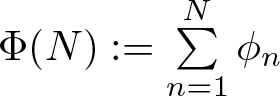 $
\Phi(N):= \sum\limits_{n=1}^{N}\phi_n
$.
A mechanism of applying Lemma A1 for proving results similar to our counting results can be found in [Reference Pollington, Velani, Zafeiropoulos and Zorin15]. We will move in parallel to their proof, taking into account that, unlike [Reference Pollington, Velani, Zafeiropoulos and Zorin15], we do not have growth conditions on the sequence  $\mathcal{A}= (q_n)_{n\in \mathbb{N}}$ and decay rate for
 $\hat{\mu}(t)$.
Choosing
$f_n(x)$ and fn from Lemma A1

Let us consider Lemma A1 with
 \begin{align}
X := \mathbb{I} \, , \qquad f_n(x):= \chi_{_{E(q_n, \gamma, \psi)}}(x) \qquad {\rm and } \qquad
f_n=2\psi(q_n) \, .
\end{align}
It follows from (5) that, with this choice of  $f_n(x)$,
 \begin{align*}
\text{the l.h.s. of } (\text{A}2) \ = \ R(x, N).
\end{align*}
Note that  $f_n(x)^2=f_n(x),$
 $x \in \mathbb{I},$ so for any
 $a,b \in \mathbb{N}$ with a < b,
 \begin{align*}
\begin{aligned}
\left(\sum_{n=a}^{b}(f_n(x)-f_n) \right)^2 &= \ \left(\sum_{n=a}^{b}f_n(x)\right)^2 \, + \, \left(\sum_{n=a}^{b}f_n\right)^2 - \ 2\sum_{n=a}^{b}f_n(x) \cdot \sum_{n=a}^{b}f_n \\[2ex]
= \ \sum_{n=a}^{b}f_n(x) \ &+ \ 2\mathop{\sum\sum}_{a\leq m \lt n\leq b}f_m(x)f_n(x) \ + \ \left(\sum_{n=a}^{b}f_n\right)^2 \ - \ 2\sum_{n=a}^{b}f_n\cdot\sum_{n=a}^{b}f_n(x) \, ,
\end{aligned}
\end{align*}
and so it follows that
 \begin{align}
\begin{aligned}
\text{the l.h.s. of } (\text{A}1)
\ = \ \sum_{n=a}^{b}\mu(E_n) \, + \, 2 &\mathop{\sum\sum}_{a\leq m \lt n\leq b} \mu(E_m\cap E_n)- \\[2ex] \, &- \ 4 \sum_{n=a}^{b} \psi(q_n) \left( \sum_{n=a}^{b}\mu(E_n) - \sum_{n=a}^{b} \psi(q_n) \right),
\end{aligned}
\end{align}
here we used the following short notation  $E_n:=E(q_n, \gamma, \psi), \quad n \in \mathbb{N}.$
Relation (A4) shows that we need to obtain a ‘good’ estimate of the measure of sets  $E_n=E(q_n, \gamma, \psi)$ and the measure of their intersections to satisfy the condition (A1).
Estimating the measure of the sets En and their intersections
In this section, we present different estimates that help us to prove the main result. We will use the Fourier analysis estimating the measure of sets En and their intersections.
Let ɛ and δ be real numbers such that  $0 \lt \varepsilon\leq 1$ and
 $0 \lt \delta \lt 1/4$. Let
 $ \chi_{\delta} : \mathbb{I} \to \mathbb{R} $ be the characteristic function defined by
 \begin{align*}
\chi_{\delta}(x):= \begin{cases}1 \ \text{if } \ \|x\|\leq \delta, \\[1ex]
0 \ \text{if } \ \|x\| \gt \delta \, , \end{cases} \end{align*}
and let  $\chi_{\delta, \varepsilon}^+ : \mathbb{I} \to \mathbb{R} $ and
 $ \chi_{\delta, \varepsilon}^-: \mathbb{I} \to \mathbb{R}$ be the continuous upper and lower approximations of χδ given by
 \begin{align*}
\chi_{\delta, \varepsilon}^+(x):= \begin{cases} 1 &\ \text{ if } \ \|x\|\leq \delta, \\[1ex]
1+ \dfrac{1}{\delta\varepsilon}(\delta-\|x\|) &\ \text{ if } \ \delta \lt \|x\| \leq (1+\varepsilon)\delta \\[1.3ex]
0 & \ \text{if } \ \|x\| \gt (1+\varepsilon)\delta \, , \end{cases} \end{align*}
and
 \begin{align*}
\chi_{\delta, \varepsilon}^-(x): = \begin{cases} 1 & \ \text{ if } \ \|x\|\leq (1 -\varepsilon)\delta \\[1ex]
\dfrac{1}{\delta\varepsilon}(\delta-\|x\|) &\ \text{ if } \ (1-\varepsilon)\delta \lt \|x\| \leq \delta \\[1.3ex]
0 & \ \text{ if } \ \|x\| \gt \delta \, . \end{cases}
\end{align*}
Clearly, both  $\chi_{\delta, \varepsilon}^+ $ and
 $ \chi_{\delta, \varepsilon}^- $ are periodic functions with period 1. Next, given a real positive function
 $\psi:\mathbb{N}\rightarrow \mathbb{I}$ and any integer
 $q\geq 4$, consider the functions
 $W_{q,\gamma,\varepsilon,\psi}^{+} $ and
 $W_{q,\gamma,\varepsilon,\psi}^{-}$ defined by
 \begin{align}
W_{q,\gamma,\varepsilon}^{+}(x)=W_{q,\gamma,\varepsilon,\psi}^{+}(x)\ :=\ \Big( \sum_{p=0}^{q-1}\delta_{\frac{p+\gamma}{q}} (x) \Big) *\chi_{\frac{\psi(q)}{q},\varepsilon}^{+}(x)
\end{align}
and
 \begin{align*}
W_{q,\gamma,\varepsilon}^{-}(x) =W_{q,\gamma,\varepsilon,\psi}^{-} (x) \ := \ \Big(\sum_{p=0}^{q-1}\delta_{\frac{p+\gamma}{q}} (x) \Big) *\chi_{\frac{\psi(q)}{q},\varepsilon}^{-} (x) \, ,
\end{align*}
where  $ * $ denotes convolution and δx denotes the Dirac delta-function at the point
 $x\in\mathbb{R}$.
It occurs that
 \begin{eqnarray*}
W_{q,\gamma,\varepsilon}^{+}(x) = \sum_{p=0}^{q-1}\chi_{\frac{\psi(q)}{q}, \varepsilon}^{+}\left(\textstyle{x- \frac{p+\gamma}{q}}\right)
\end{eqnarray*}
and
 \begin{eqnarray*}
W_{q,\gamma,\varepsilon}^{-}(x) = \sum_{p=0}^{q-1}\chi_{\frac{\psi(q)}{q}, \varepsilon}^{-}\left(\textstyle{x- \frac{p+\gamma}{q}}\right) \, .
\end{eqnarray*}
It thus follows that for any  $0 \lt \varepsilon \le 1$ and any integer
 $q\geq 4$,
 \begin{align}
\int_{0}^{1}W_{q,\gamma,\varepsilon}^-(x)\mathrm{d}\mu(x)
\; \leq \;
\mu( E(q, \gamma, \psi)) \; \leq \; \int_{0}^{1}W_{q,\gamma,\varepsilon}^+(x)\mathrm{d}\mu(x). \end{align}
Now we need to consider the Fourier series expansions
 \begin{align*} \sum_{k \in \mathbb{Z} }\widehat{W}_{q,\gamma,\varepsilon}^{\pm}(k) \exp(2\pi kix)
\end{align*}
of  $ W_{q,\gamma,\varepsilon}^{+} $ and
 $W_{q,\gamma,\varepsilon}^{-} $.
The values and basic estimates of the Fourier coefficients  $\widehat{W}_{q,\gamma,\varepsilon}^{\pm}(k)$ are presented in [Reference Pollington, Velani, Zafeiropoulos and Zorin15] (see Lemma 1 in [Reference Pollington, Velani, Zafeiropoulos and Zorin15]). For the convenience of the reader, we collect them in the following proposition.
Proposition A2. Let  $0 \lt \varepsilon,\tilde{\varepsilon} \le 1$ and
 $\widehat{W}_{q,\gamma,\varepsilon}^{\pm}(k), \quad k \in \mathbb{Z},$ are the Fourier coefficients of
 $ W_{q,\gamma,\varepsilon}^{+} $ and
 $W_{q,\gamma,\varepsilon}^{-} $. Then, for any integers
 $q, r \geq 4:$
(i) for k ≠ 0,
 \begin{align}
\widehat{W}_{q,\gamma,\varepsilon}^+(k)\, =\,\begin{cases}
\exp\left( -\dfrac{2\pi i k \gamma}{q}\right) \dfrac{q\left(\cos(2\pi k\psi(q)q^{-1})-\cos(2\pi k\psi(q)q^{-1}(1+\varepsilon))\right)}{2\pi^2 k^2\psi(q)q^{-1}\varepsilon} &\text{\ if } \ q\mid k \\[3ex]
0 & \text{\ if } \ q\nmid k \, ,
\end{cases} \,
\end{align}
and for k = 0,
 \begin{align}
\widehat{W}_{q,\gamma,\varepsilon}^{+}(0)=(2+\varepsilon) \, \psi(q)\, ;
\end{align}
(ii) for k ≠ 0,
 \begin{align}
\widehat{W}_{q,\gamma,\varepsilon}^-(k)\, =\,
\begin{cases}
\exp\left( -\dfrac{2\pi i k \gamma}{q}\right) \dfrac{q\left(\cos(2\pi k\psi(q)q^{-1}(1-\varepsilon))-\cos(2\pi k\psi(q)q^{-1}) \right)}{2\pi^2 k^2\psi(q)q^{-1}\varepsilon} &\text{\ if } \ q\mid k \\[3ex]
0 & \text{\ if } \ q\nmid k \, ,
\end{cases}
\end{align}
and for k = 0,
 \begin{align}
\widehat{W}_{q,\gamma,\varepsilon}^-(0) = (2 - \varepsilon)\, \psi(q) \, ;
\end{align}
(iii) for any  $ s\in\mathbb{Z} \setminus\{0\} $
 \begin{eqnarray}
\left|\widehat{W}_{q,\gamma,\varepsilon}^{\pm}(s q)\right| &\leq& (2+\varepsilon) \, \psi(q),
\end{eqnarray}
 \begin{eqnarray}
\left|\widehat{W}_{q,\gamma,\varepsilon}^{\pm}(s q)\right| &\leq& \frac{1}{\pi^2s^2\psi(q)\varepsilon}.
\end{eqnarray}
(iv)
 \begin{eqnarray}
\sum_{s \in \mathbb{Z}} \big|\widehat{W}_{q,\gamma,\varepsilon}^{\pm}(sq)\big| \ \lt \ \frac{3}{\varepsilon^{1/2}}
\end{eqnarray}
and
 \begin{align}
\sum_{s\in \mathbb{Z}} \, \sum_{t\in \mathbb{Z}} \, \big|\widehat{W}_{q,\gamma,\varepsilon}^{\pm}(sq)\big| \ \big|\widehat{W}_{r,\gamma,\tilde{\varepsilon}}^{\pm}(tr)\big| \ \leq \ \frac{9}{\varepsilon^{1/2}\cdot\tilde{\varepsilon}^{1/2}} \, .
\end{align}
By (A13),  $\sum\limits_{k \in \mathbb{Z}} \big| \widehat{W}_{q,\gamma,\varepsilon}^{\pm}(k) \big| \lt \infty $, so the Fourier series
 \begin{align*} \sum_{k \in \mathbb{Z} }\widehat{W}_{q,\gamma,\varepsilon}^{\pm}(k) \exp(2\pi kix)
\end{align*}
converges uniformly to  $W_{q,\gamma,\varepsilon}^{\pm}(x)$ for all
 $ x \in \mathbb{I}$. Hence, it follows that
 \begin{eqnarray*}
\int_0^1 W_{q,\gamma,\varepsilon}^{\pm}(x) \; \mathrm{d}\mu(x) \; = \; \sum_{k\in \mathbb{Z}} \, \widehat{W}_{q,\gamma,\varepsilon}^{\pm}(k) \; \widehat{\mu}(-k) \, .
\end{eqnarray*}
This together with (A6), (A8), (A10) and the fact that  $\widehat{\mu}(0)=1$, implies that
 \begin{align}
\begin{array}{ll}
\mu( E(q, \gamma, \psi)) \ \leq \ (2+\varepsilon) \, \psi(q) \ + \displaystyle{\sum_{k \in \mathbb{Z} \setminus \{0 \} }}\widehat{W}_{q,\gamma,\varepsilon}^{+}(k) \; \widehat{\mu}(-k)\;
\\[6ex]
\mu( E(q, \gamma, \psi)) \ \geq \ (2-\varepsilon) \, \psi(q) \ + \displaystyle{\sum_{k \in \mathbb{Z} \setminus \{0 \} }} \widehat{W}_{q,\gamma,\varepsilon}^{-}(k) \; \widehat{\mu}(-k) \, .
\end{array} \,
\end{align}
Estimating the sums from measures of En
Now we are ready to prove the following estimates for the sums of  $\mu(E_n).$
Lemma A3. Under the conditions of Theorem 4, we have, for arbitrary  $a,b \in \mathbb{N}$ with a < b,
 \begin{align}
\sum_{n=a}^b\mu(E(q_n, \gamma, \psi)) = 2\sum_{n=a}^b\psi(q_n) \, + \, O\left( \min\Big(1,\sum_{n=a}^b\psi(q_n)\Big) \right).
\end{align}
We need the following well-known statement in order to prove Lemma A3. We will leave this statement without citation because, in our opinion, it belongs to the mathematical folklore.
Lemma A4. Let  $(a_n)_{n \in \mathbb{N}}$ be a sequence of nonnegative real numbers verifying
 $a_1 \gt 0$ and
 \begin{align*}S_n=a_1+a_2+ \ldots + a_n, \quad n \in \mathbb{N}.\end{align*}
Then for any real ξ > 0 the series
 \begin{align*}\sum_{n=1}^{\infty}\frac{a_n}{S_n^{1+\xi}}\end{align*}
converges.
Proof of Lemma A4
Firstly, note that, for any  $n \in \mathbb{N}$,
 \begin{align}
\int_{S_{n-1}}^{S_n} \frac{dx}{x^{1+\xi}} \ge \int_{S_{n-1}}^{S_n} \frac{dx}{S_n^{1+\xi}}=\frac{a_n}{S_n^{1+\xi}}.
\end{align}
To prove the convergence of the series
 \begin{align*}\sum_{n=1}^{\infty}\frac{a_n}{S_n^{1+\xi}}\end{align*}
consider its partial sum
 \begin{align*}B_N=\sum_{n=1}^{N}\frac{a_n}{S_n^{1+\xi}}.\end{align*}
In view of (A17), for any  $N \in \mathbb{N},$
 \begin{align*}B_N=\frac{a_1}{S_1^{1+\xi}}+ \frac{a_2}{S_2^{1+\xi}} +\frac{a_3}{S_3^{1+\xi}} + \ldots +\frac{a_N}{S_N^{1+\xi}} \le\end{align*}
 \begin{align*}\le \frac{a_1}{S_1^{1+\xi}} + \int_{S_1}^{S_2} \frac{dx}{x^{1+\xi}} +\int_{S_2}^{S_3} \frac{dx}{x^{1+\xi}} +\ldots +\int_{S_{N-1}}^{S_N} \frac{dx}{x^{1+\xi}}= \frac{1}{a_1^{\xi}} + \int_{S_1}^{S_N} \frac{dx}{x^{1+\xi}}=\end{align*}
 \begin{align*}=\frac{1}{a_1^{\xi}} + \frac{1}{\xi} \left(\frac{1}{S_1^{\xi}}-\frac{1}{S_N^{\xi}}\right) \le \frac{1}{a_1^{\xi}}\left(1+\frac{1}{\xi}\right).\end{align*}
So, the sequence of partial sums  $(B_N)_{N\in \mathbb{N}}$ for the series with nonnegative elements is bounded, which implies the convergence of this series.
Now we can prove Lemma A3.
Proof of Lemma A3
We prove Lemma A3 under a weaker condition on the number ρ from (10), compared to Theorem 4, namely  $\rho \gt \frac{3}{2}$. For any given sequence of real numbers
 $(\varepsilon_n)_{n=a}^b$ in
 $(0,1]$, it follows from (A15) that
 \begin{align}
\left|\mu(E_n)-2\psi(q_n)\right| \leq \psi(q_n)\varepsilon_n+
\max_{\circ\in\{+,-\}}\left|\sum_{k\in \mathbb{Z} \setminus \{0\}}\widehat{W}_{q_n,\gamma,\varepsilon_n}^{\circ}(k)\widehat{\mu}(-k)\right|, \quad a \le n \le b.
\end{align}
It follows from (A7) and (A9) that  $\widehat{W}_{q_n,\gamma,\varepsilon_n}^{\pm}(k)=0$ unless
 $k = s q_n$ for some integer
 $s.$ Also from (11) we have, that
 $ |\widehat{\mu}(sq_n)| \ll n^{-\rho}, $ where
 $\rho \gt \frac{3}{2}.$ So, using (A13),
 \begin{align}
\left|\sum_{k\in \mathbb{Z} \setminus \{0\}}\widehat{W}_{q_n,\gamma,\varepsilon_n}^{\pm}(k)\widehat{\mu}(-k)\right| \le \sum_{s \in \mathbb{Z}\setminus \{0\}} \big|\widehat{W}_{q,\gamma,\varepsilon}^{\pm}(sq)\big| \big|\widehat{\mu}(sq_n)\big|\ll \frac{3}{n^{\rho}\varepsilon_n^{\frac{1}{2}}}.
\end{align}
Now, in view of (A18) and (A19),
 \begin{align}
\left|\sum_{n=a}^b\mu(E_n)-2\sum_{n=a}^b\psi(q_n)\right|\ll \sum_{n=a}^b\psi(q_n)\varepsilon_n+\sum_{n=a}^b\frac{3}{n^{\rho}\varepsilon_n^{\frac{1}{2}}},
\end{align}
therefore, for  $\varepsilon_n=1,$
 $a \leq n \leq b$,
 \begin{align}
\left|\sum_{n=a}^b\mu(E_n)-2\sum_{n=a}^b\psi(q_n)\right|\ll\sum_{n=a}^b\psi(q_n) \, .
\end{align}
To complete the proof, we need to get one more upper bound, namely
 \begin{align}
\left|\sum_{n=a}^b\mu(E_n)-2\sum_{n=a}^b\psi(q_n)\right|\ll 1.
\end{align}
We can deduce the upper bound (A22) again from (A20) choosing suitable values of  $(\varepsilon_n)_{n=a}^b.$ Since
 $\rho \gt \frac{3}{2},$ let us choose a real number
 $\xi \in (0, \, 2\rho -3).$ For any
 $n\in\mathbb{N}$ let
 \begin{align*}
\Psi(n):=\sum_{k=1}^n\psi(q_k) \quad {\rm and } \quad \varepsilon_n:=\min\left(1,\Psi(n)^{-1-\xi}\right).
\end{align*}
By definition,  $|\psi(q_n)|\leq 1$ and so
 $
\varepsilon_n^{-1}\leq n^{1+\xi} \, .
$ So, for the second term on the r.h.s. of (A20) we have
 \begin{align}
\sum_{n=a}^b\frac{3}{n^{\rho}\varepsilon_n^{1/2}} \, \leq \, \sum_{n=1}^\infty\frac{3}{n^{\rho - \frac{\xi}{2}-\frac{1}{2}}} \, \lt \, \infty \,,
\end{align}
since  $\rho - \frac{\xi}{2}-\frac{1}{2} \gt 1$ because of the choice of ξ.
It follows from Lemma A4 that, for ξ > 0, the series
 \begin{align*}\sum_{n=1}^{\infty}\frac{\psi(q_n)}{\Psi(n)^{1+\xi}}\end{align*}
converges, so
 \begin{align*}\sum_{n=1}^{\infty}\frac{\psi(q_n)}{\max\left(1,\Psi(n)^{1+\xi}\right)}\end{align*}
converges also. Therefore,
 \begin{align}
\sum_{n=a}^b\psi(q_n)\varepsilon_n \, \lt \, \sum_{n=1}^{\infty}\frac{\psi(q_n)}{\max\left(1,\Psi(n)^{1+\xi}\right)} \, \lt \, \infty \, .
\end{align}
The upper bound (A22) now follows from the inequalities (A20), (A23) and (A24).
Estimating the sums from measures of intersections
$E_n \cap E_m$

Estimating the sums from measures of intersections of the sets En is technically a more complicated work. Here, we use the condition on α-separability (see Definition 2), which we do not use proving Lemma A3.
Before formulating the statement on the upper bound for the sums of measures of intersections, we prove the following result, related to the case ξ = 0 of Lemma A4.
Lemma A5. Let  $(a_n)_{n \in \mathbb{N}}$ be a sequence of nonnegative real numbers,
 $a_1 \ne 0$ and
 \begin{align*}S_n=a_1+a_2+ \ldots + a_n, \quad n \in \mathbb{N}.\end{align*}
Then for any  $N \in \mathbb{N}$ for the partial sums BN of the series
 \begin{align*}\sum_{n=1}^{\infty}\frac{a_n}{S_n}\end{align*}
we have
 \begin{align*}B_N=\sum_{n=1}^{N}\frac{a_n}{S_n} \le 1+ \log(S_N) - \log(a_1).\end{align*}
Proof of Lemma A5
First note that for any  $n \in \mathbb{N}$
 \begin{align}
\int_{S_{n-1}}^{S_n} \frac{dx}{x} \ge \int_{S_{n-1}}^{S_n} \frac{dx}{S_n}=\frac{a_n}{S_n}.
\end{align}
In view of (A25), for any  $N \in \mathbb{N},$
 \begin{align*}B_N=\frac{a_1}{S_1}+ \frac{a_2}{S_2} +\frac{a_3}{S_3} + \ldots +\frac{a_N}{S_N} \le\end{align*}
 \begin{align*}\le \frac{a_1}{S_1} + \int_{S_1}^{S_2} \frac{dx}{x} +\int_{S_2}^{S_3} \frac{dx}{x} +\ldots +\int_{S_{N-1}}^{S_N} \frac{dx}{x}= 1 + \int_{S_1}^{S_N} \frac{dx}{x}=\end{align*}
 \begin{align*}= 1+ \log(S_N) - \log(S_1) = 1+ \log(S_N) - \log(a_1).\end{align*}
Now we can formulate and prove the statement on the upper bound for the sums from measures of intersections.
Lemma A6. Let for any τ > 1
 \begin{align}
\psi(q_n) \ge n^{-\tau}, \quad n \in \mathbb{N}.
\end{align}
Then, under all conditions of Theorem 4, for arbitrary  $a,b \in \mathbb{N}$ with a < b,
 \begin{align}\begin{aligned}
2 \mathop{\sum\sum}_{a\leq m \lt n\leq b} \mu(E_m\cap E_n) \ \leq \ \left( \sum_{n=a}^{b} \mu(E_n) \right)^2 + O\left(\mathop{\sum\sum}_{a\leq m \lt n\leq b} (q_m,q_n)\min\left(\frac{\psi(q_m)}{q_m},\frac{\psi(q_n)}{q_n}\right)\right) \\[2ex]
+ O\left(\left(\sum_{n=a}^{b}\psi(q_n)\right)\log^+\left(\sum_{n=a}^{b}\psi(q_n)\right)+\sum_{n=a}^{b}\psi(q_n)\right),
\end{aligned}
\end{align}
where  $\log^+(x):=\max(0,\log(x)), \quad x \gt 0.$
Proof of Lemma A6
In order to receive suitable estimates of the measures of intersections, we start with some Fourier analysis (once again, we move here in parallel with the corresponding reasoning in [Reference Pollington, Velani, Zafeiropoulos and Zorin15]). So, let us fix a sequence of real numbers  $(\varepsilon_n)_{n\in \mathbb{N}} \subset (0,1]$ and consider the functions
 \begin{align}
W_{m,n}^{+}(x):= W_{q_m,\gamma,\varepsilon_m}^+(x) \cdot W_{q_n,\gamma,\varepsilon_n}^+(x), \quad x \in \mathbb{R}, \, m,n \in \mathbb{N}, \, m \lt n,
\end{align}
(recall that the function  $W_{q,\gamma,\varepsilon}^{+}$ is defined by (A5)). Then,
 \begin{eqnarray*}
\mu(E_m\cap E_n) &\leq& \int_{0}^{1} W_{q_m,\gamma,\varepsilon_m}^+(x) W_{q_n,\gamma,\varepsilon_n}^+(x) \, \mathrm{d}\mu(x) \nonumber
\\ [2ex]
&=& \int_{0}^{1}W_{m,n}^{+}(x)\mathrm{d}\mu(x).
\end{eqnarray*}
The Fourier coefficients of the product  $W_{m,n}^{+}$ are convolutions
 \begin{eqnarray}
\widehat{W}_{m,n}^{+}(k) & := & \, \int_{0}^{1}
W_{q_m,\gamma,\varepsilon_m}^{+}(x)W_{q_n,\gamma,\varepsilon_n}^{+}(x) \, \exp(-2\pi kix) \mathrm{d}x \nonumber \\[2ex]
& = & \sum_{j \in \mathbb{Z}} \widehat{W}_{q_m,\gamma,\varepsilon_m}^{+}(j) \
\widehat{W}_{q_n,\gamma,\varepsilon_n}^{+}(k-j), \quad k \in \mathbb{Z}.
\end{eqnarray}
Moreover,  $\sum\limits_{k \in \mathbb{Z}} \big| \widehat{W}_{m,n}^{+}(k) \big| \lt \infty $, so the Fourier series
 \begin{align*} \sum_{k \in \mathbb{Z} }\widehat{W}_{m,n}^{+}(k) \exp(2\pi kix)
\end{align*}
converges uniformly to  $W_{m,n}^{+}(x)$ for all
 $ x \in \mathbb{I}$. Hence, it follows that
 \begin{eqnarray*}
\int_0^1 W_{m,n}^{+}(x) \; \mathrm{d}\mu(x) \; = \; \sum_{k\in \mathbb{Z}} \, \widehat{W}_{m,n}^{+}(k) \; \widehat{\mu}(-k) \, .
\end{eqnarray*}
So,
 \begin{eqnarray}
\mu(E_m\cap E_n) = \mu (E(q_m, \gamma, \psi) \cap E(q_n, \gamma, \psi))&\leq& \qquad \qquad \qquad\qquad \qquad\qquad
\end{eqnarray}
 \begin{eqnarray*}
\leq \sum_{k \in \mathbb{Z} }\widehat{W}_{m,n}^{+}(k)\widehat{\mu}(-k) \nonumber
&=& \widehat{W}_{m,n}^{+}(0) + \sum_{k\in \mathbb{Z} \setminus \{0\}} \widehat{W}_{m,n}^{+}(k)\widehat{\mu}(-k).
\end{eqnarray*}
We consider the two terms on the right-hand side of (A30) separately. From (A29) with  $k=0,$ (and refer to (3)) we have
 \begin{align}
\begin{aligned}
\widehat{W}_{m,n}^{+}(0) &:= \, \int_{0}^{1}W_{q_m,\gamma,\varepsilon_m}^{+}(x)W_{q_n,\gamma,\varepsilon_n}^{+}(x)\mathrm{d}x \leq \\[2ex]
&\leq \, \Big|E\left(q_m, \gamma, (1+\varepsilon_m)\cdot \psi\right) \cap E\left(q_m, \gamma, (1+\varepsilon_n)\cdot \psi\right)\Big|\, ,
\end{aligned}
\end{align}
where  $ | \, . \, | $ is Lebesgue measure. It is relatively straightforward to verify (see [Reference Harman8, Equation 3.2.5]Footnote 2 for the details) that for any
 $q, q' \in \mathbb{N}$
 \begin{align*}
| E(q, \gamma, \psi) \cap E(q', \gamma, \psi)| \, = \, 4\psi(q)\psi(q')+ O\left( (q,q') \ \min\Big(\frac{\psi(q)}{q},\frac{\psi(q')}{q'}\Big) \right) \, .
\end{align*}
Hence, it follows that
 \begin{align*}\begin{aligned}
\Big|E\left(q_m, \gamma, (1+\varepsilon_m)\cdot \psi\right) \cap E\left(q_m, \gamma, (1+\varepsilon_n)\cdot \psi\right)\Big| \, = \, 4(1+\varepsilon_m)(1+\varepsilon_n)\psi(q_m)\psi(q_n) \\[1ex] + \ \ O\left( (q_m,q_n)\min\Big(\frac{\psi(q_m)}{q_m},\frac{\psi(q_n)}{q_n}\Big) \right) \, .
\end{aligned}
\end{align*}
This together with (A31) implies that
 \begin{align}
\widehat{W}_{m,n}^{+}(0) \, \leq \, 4(1+\varepsilon_m)(1+\varepsilon_n)\psi(q_m)\psi(q_n) + O\left( (q_m,q_n)\min\Big(\frac{\psi(q_m)}{q_m},\frac{\psi(q_n)}{q_n}\Big) \right) \, ,
\end{align}
which gives us the estimate of the first term on the right-hand side of (A31).
We proceed with considering the second term, which we will denote by  $S_{m,n}$. In view of (A7) and (A29), it follows that
 \begin{eqnarray}
S_{m,n} &:= & \sum_{k \in\mathbb{Z}\setminus \{0\} } \widehat{W}_{m,n}^{+}(k)\widehat{\mu}(-k) = \nonumber \\[2ex]
&= & \mathop{\mathop{\sum\sum}_{s,t\in\mathbb{Z} } }_{sq_m-tq_n \neq 0}
\widehat{W}_{q_m,\gamma,\varepsilon_m}^{+}(sq_m)
\widehat{W}_{q_n,\gamma,\varepsilon_n}^{+}(tq_n)
\widehat{\mu}\left(-(sq_m+tq_n)\right).
\end{eqnarray}
We decompose  $S_{m,n}$ into three sums:
 \begin{align*}
S_{m,n}= S_1(m,n)+S_2(m,n)+S_3(m,n),
\end{align*}
where
 \begin{eqnarray*}
S_1(m,n) &:=& \sum_{t\in \mathbb{Z} \setminus \{0\}} \widehat{W}_{q_m,\gamma,\varepsilon_m}^+(0) \widehat{W}_{q_n,\gamma,\varepsilon_n}^{+}(tq_n)\widehat{\mu}(-tq_n), \\[2ex]
S_2(m,n) &:=& \sum_{s\in \mathbb{Z} \setminus \{0\}} \widehat{W}_{q_n,\gamma,\varepsilon_n}^+(0) \widehat{W}_{q_m,\gamma,\varepsilon_m}^{+}(sq_m)\widehat{\mu}(-sq_m), \\[2ex]
S_3(m,n) &:=& \mathop{\mathop{\sum\sum}_{s,t\in\mathbb{Z}\setminus \{0\} } }_{sq_m+tq_n\neq 0}\widehat{W}_{q_m,\gamma,\varepsilon_m}^{+}(sq_m)\widehat{W}_{q_n,\gamma,\varepsilon_n}^{+}(tq_n)\widehat{\mu}\left(-(sq_m+tq_n)\right).
\end{eqnarray*}
Inequalities (A8), (A13) and balance condition (11) imply that, for any  $m,n \in \mathbb{N},$ m < n,
 \begin{align}
|S_1(m,n)| \ \ll \ \frac{(2+\varepsilon_m)\psi(q_m)}{n^{\rho}}\sum_{t\in \mathbb{Z} } \widehat{W}_{q_n,\gamma,\varepsilon_n}^{+}(tq_n) \ \ll \
\frac{\psi(q_m)}{n^{\rho}\varepsilon_n^{1/2}}\, .
\end{align}
Symmetrically, for any  $m,n \in \mathbb{N},$
 $m \lt n,$
 \begin{align}
|S_2(m,n)| \ \ll \
\frac{\psi(q_n)}{m^{\rho}\varepsilon_m^{1/2}}\, .
\end{align}
Now we decompose S 3 into two sums:
 \begin{align*} S_3(m,n) \, =\, S_4(m,n) + S_5(m,n), \end{align*}
where
 \begin{align*} S_4(m,n) \ := \mathop{\mathop{\sum\sum}_{s,t\in\mathbb{Z}\setminus \{0\} } }_{|sq_m-tq_n|\geq q_m^{\alpha}} \! \widehat{W}_{q_m,\gamma,\varepsilon_m}^{+}(-sq_m)\widehat{W}_{q_n,\gamma,\varepsilon_n}^{+}(tq_n) \widehat{\mu}\left( sq_m-tq_n\right) \end{align*}
and
 \begin{align}
S_5(m,n) \ := \mathop{\mathop{\sum\sum}_{s,t\in\mathbb{Z}\setminus \{0\} } }_{1\leq |sq_m-tq_n| \lt q_m^{\alpha}} \!\!\!\! \widehat{W}_{q_m,\gamma,\varepsilon_m}^{+}(-sq_m)\widehat{W}_{q_n,\gamma,\varepsilon_n}^{+}(tq_n) \widehat{\mu}\left( sq_m-tq_n\right),
\end{align}
here  $\alpha \in (0,1)$ is the constant from α-separability condition of Theorem 4. Regarding S 4, by making use of the balance condition (11) with the restriction
 $|sq_m-tq_n|\geq q_m^{\alpha}$ and inequality (A14), it follows that
 \begin{align}
|S_4(m,n)| \ \ll \ \frac{1}{m^{\rho}}\mathop{\sum\sum}_{s,t\in\mathbb{Z}\setminus \{0\} }
\left|\widehat{W}_{q_m,\gamma,\varepsilon_m}^{+}(-sq_m)\right| \left|\widehat{W}_{q_n,\gamma,\varepsilon_n}^{+}(tq_n)\right| \ \ll \
\frac{1}{m^{\rho}\varepsilon_m^{1/2}\varepsilon_n^{1/2}}\, .
\end{align}
Finally, we decompose S 5 into two sums:
 \begin{align*} S_5(m,n) \, =\, S_6(m,n) + E(m,n), \end{align*}
where
 \begin{align*} S_6(m,n):= \mathop{\mathop{\mathop{\sum\sum}_{s,t\in\mathbb{Z}\setminus \{0\} } }_{s \gt m^3/\psi(q_m)}}_{1\leq |sq_m-tq_n| \lt q_m^{\alpha}} \widehat{W}_{q_m,\gamma,\varepsilon_m}^{+}(-sq_m)\widehat{W}_{q_n,\gamma,\varepsilon_n}^{+}(tq_n) \widehat{\mu}\left( sq_m-tq_n\right) \,
\end{align*}
and
 \begin{align*} E(m,n):= \mathop{\mathop{\mathop{\sum\sum}_{s,t\in\mathbb{Z}\setminus \{0\} } }_{1\leq s \leq m^3/\psi(q_m)}}_{1\leq |sq_m-tq_n| \lt q_m^{\alpha}} \widehat{W}_{q_m,\gamma,\varepsilon_m}^{+}(-sq_m)\widehat{W}_{q_n,\gamma,\varepsilon_n}^{+}(tq_n) \widehat{\mu}\left( sq_m-tq_n\right).
\end{align*}
The restriction  $1 \leq |sq_m-tq_n| \lt q_m^{\alpha}$ implies that
 \begin{align}
0 \lt \left|s-t\frac{q_n}{q_m}\right| \lt 1 \, .
\end{align}
Hence, if nonzero s and t satisfy (A38), then both necessarily must have the same sign, and also for each fixed integer s there exists a set Ts of at most two non-zero integers t satisfying the restriction  $1 \leq |sq_m-tq_n| \lt q_m^{\alpha}.$ So, we can write S 6 as a single sum
 \begin{align*}S_6(m,n)= \mathop{\mathop{\sum}_{s \gt m^3/\psi(q_m) : } }_{t \in T_s}
\widehat{W}_{q_m,\gamma,\varepsilon_m}^{+}(-sq_m) \widehat{W}_{q_n,\gamma,\varepsilon_n}^{+}(tq_n)\widehat{\mu}\left( sq_m-tq_n\right).\end{align*}
So, using the trivial bound  $|\widehat{\mu}(t)| \leq 1 $ together with (A11) to bound
 $|\widehat{W}_{q_n,\gamma,\varepsilon_n}^{+}(t q_n)|$ and (A12) to bound
 $ |\widehat{W}_{q_m,\gamma,\varepsilon_n}^{+}(sq_m)| $, we obtain that for any integers
 $ 1 \leq m \lt n $
 \begin{eqnarray}
|S_6(m,n)| & \ll & \mathop{\mathop{\sum}_{s \gt m^3/\psi(q_m) : } }_{t \in T_s}
|\widehat{W}_{q_m,\gamma,\varepsilon_m}^{+}(sq_m)| \ | \widehat{W}_{q_n,\gamma,\varepsilon_n}^{+}(tq_n)| \nonumber
\\[2ex]
& \ll & \sum_{s \gt m^3/\psi(q_m)}\frac{1}{s^2\psi(q_m) \, \varepsilon_m }\psi(q_n) \ \ll \ \frac{\psi(q_n)}{m^3 \, \varepsilon_m } \, .
\end{eqnarray}
Working with  $E(m,n)$ note, that in view of (A26) the condition
 $s \leq m^3/\psi(q_m)$ implies that
 $s \le m^5.$ This, together with the fact that
 $(q_n)_{n\in\mathbb{N}}$ is α-separated implies that
 $E(m,n)$ is empty sum. Thus,
 \begin{align}
E(m,n)=0.
\end{align}
So, from upper bounds (A34), (A35), (A37), (A39), and equality (A40), for any fixed  $a,b \in \mathbb{N}$ with
 $a \lt b,$ and all natural numbers
 $m,n,$ with
 $a\leq m \lt n\leq b:$
 \begin{align}
|S_{m,n}| \ll \frac{\psi(q_m)}{n^{\rho}\varepsilon_n^{1/2}}\, + \frac{\psi(q_n)}{m^{\rho}\varepsilon_m^{1/2}}\, + \frac{1}{m^{\rho}\varepsilon_m^{1/2}\varepsilon_n^{1/2}}\, + \frac{\psi(q_n)}{m^3 \, \varepsilon_m } \,.
\end{align}
Now, given  $a\in\mathbb{N}$, define, for all
 $n\in\mathbb{N}$,
 $n\geq a$,
 \begin{align}
\varepsilon_n:=\min\left(1,\, \left( \sum_{k=a}^{n}\psi(q_k) \right)^{-1}\right).
\end{align}
Then, since  $\psi(k) \le 1$ for all
 $k \in \mathbb{N}$,
 \begin{align}
\varepsilon_n^{-1} \, \leq \, \max\left(1,n\right) \, \le \, n, \quad n \ge a.
\end{align}
Therefore,
 \begin{align*}\sum_{n=a}^{\infty}\frac{1}{n^{\rho}\varepsilon_n^{1/2}} \, \le \, \sum_{n=a}^{\infty}\frac{1}{n^{\rho-\frac{1}{2}}} \, \lt \, \infty \, ,\end{align*}
(recall that ρ > 2), and so, it follows from (A41) that for any  $a,b \in \mathbb{N},$
 $a \lt b,$
 \begin{align}
\mathop{\sum\sum}_{a\leq m \lt n\leq b}|S_{m,n}| \, \ll \, \sum_{n=a}^{b} \psi(q_n) + \mathop{\sum\sum}_{a\leq m \lt n\leq b}\frac{1}{n^{\rho}\varepsilon_m^{1/2}\varepsilon_n^{1/2}} + \mathop{\sum\sum}_{a\leq m \lt n\leq b}\frac{\psi(q_n)}{m^3 \, \varepsilon_m } \,.
\end{align}
For the third sum in the right-hand side of (A44), from inequalities (A43), we have
 \begin{align}
\mathop{\sum\sum}_{a\leq m \lt n\leq b}\frac{\psi(q_n)}{m^3 \, \varepsilon_m } \le \mathop{\sum\sum}_{a\leq m \lt n\leq b}\frac{\psi(q_n)}{m^2} \ll
\sum_{n=a}^{b} \psi(q_n), \quad a,b \in \mathbb{N}, \, a \lt b.
\end{align}
In order to estimate the second sum in the right-hand side of (A44), let us consider two cases.
Case 1:  $\sum\limits_{k=a}^{b}\psi(q_k) \gt 1$. Then, by (A42),
 \begin{align*} \frac{1}{n^{\rho}\varepsilon_m^{1/2}\varepsilon_n^{1/2}} \leq \frac{1}{n^{\rho}}\sum_{k=a}^{b}\psi(q_k),\end{align*}
and so, since  $\rho \gt 2,$
 \begin{align}
\mathop{\sum\sum}\limits_{a\leq m \lt n\leq b} \frac{1}{n^{\rho}\varepsilon_m^{1/2}\varepsilon_n^{1/2}} \leq \left(\mathop{\sum\sum}\limits_{a\leq m \lt n\leq b} \frac{1}{n^{\rho}}\right) \cdot \left(\sum_{k=a}^{b}\psi(q_k)\right) \ll \sum_{k=a}^{b}\psi(q_n).
\end{align}
Case 2:  $\sum\limits_{k=a}^{b}\psi(q_k) \le 1$. It follows, by (A42), that
 $\varepsilon_n=1$ for all
 $a\leq n\leq b$, therefore
 \begin{align*}
\frac{1}{n^{\rho}\varepsilon_m^{1/2}\varepsilon_n^{1/2}} = \frac{1}{n^{\rho}}.
\end{align*}
By using Lemma A6 with  $\tau = \frac{\rho}{2}$, we get
 \begin{align*}\frac{1}{n^{\rho}\varepsilon_m^{1/2}\varepsilon_n^{1/2}} = \frac{1}{n^{\rho}}\leq\frac{\psi(q_n)}{n^{\frac{\rho}{2}}}, \quad \ n \in \mathbb{N}, \end{align*}
and so
 \begin{align}
\mathop{\sum\sum}\limits_{a\leq m \lt n\leq b} \frac{1}{n^{\rho}\varepsilon_m^{1/2}\varepsilon_n^{1/2}} \leq \mathop{\sum\sum}\limits_{a\leq m \lt n\leq b} \frac{\psi(q_n)}{n^{\frac{\rho}{2}}} \leq \mathop{\sum\sum}\limits_{a\leq m \lt n\leq b} \frac{\psi(q_n)}{m^{\frac{\rho}{2}}} \ll \sum_{n=a}^b\psi(q_n).
\end{align}
Both cases give us the same upper bound. So, estimates (A45), (A46) and (A47), together with (A44), imply that, for all  $a,b \in \mathbb{N}$ with a < b,
 \begin{align*}
\mathop{\sum\sum}_{a\leq m \lt n\leq b}|S_{m,n}| \, \ll \, \sum_{n=a}^{b}\psi(q_n) \, .
\end{align*}
Therefore, by (A30),
 \begin{align}
\mathop{\sum\sum}\limits_{a\leq m \lt n\leq b}\mu(E_m\cap E_n) \leq \mathop{\sum\sum}\limits_{a\leq m \lt n\leq b}\widehat{W}_{m,n}^{+}(0)+ O\left(\sum_{n=a}^{b}\psi(q_n) \right) .
\end{align}
We now turn our attention to estimating the first term on the right-hand side of (A48). Recall that according to (A32)
 \begin{align*}
\widehat{W}_{m,n}^{+}(0) \, \leq \, 4(1+\varepsilon_m)(1+\varepsilon_n)\psi(q_m)\psi(q_n) + O\left( (q_m,q_n)\min\Big(\frac{\psi(q_m)}{q_m},\frac{\psi(q_n)}{q_n}\Big) \right) \,.
\end{align*}
Since  $(\varepsilon_n)_{n \ge a}$ is decreasing and
 $\varepsilon_n \le 1,$
 $n \ge a,$ for all
 $m,n \in \mathbb{N}$ with
 $a\le m \lt n \le b,$
 \begin{align}
4(1+\varepsilon_m)(1+\varepsilon_n)\psi(q_m)\psi(q_n) \, \leq \, 4\psi(q_m)\psi(q_n) + 12 \varepsilon_m \psi(q_m) \psi(q_n) \, .
\end{align}
Once again, we will consider two cases.
Case 1:  $\sum\limits_{k=a}^b\psi(q_k)\le 1$. It follows, by (A42), that
 $\varepsilon_n=1$ for all
 $a\leq n\leq b$, therefore
 \begin{align}
\mathop{\sum\sum}\limits_{a\leq m \lt n\leq b} \varepsilon_m\psi(q_m)\psi(q_n)\leq \mathop{\sum\sum}\limits_{a\leq m \lt n\leq b}\psi(q_m)\psi(q_n) \lt \left(\sum_{n=a}^b\psi(q_n)\right)^2 \lt \sum_{n=a}^b\psi(q_n).
\end{align}
Case 2:  $\sum\limits_{k=a}^b\psi(q_k) \gt 1 $. Then, by (A42),
 \begin{align}
\begin{aligned}
\mathop{\sum\sum}\limits_{a\leq m \lt n\leq b} &\varepsilon_m\psi(q_m)\psi(q_n)= \mathop{\sum\sum}\limits_{a\leq m \lt n\leq b} \psi(q_m)\psi(q_n)\ \min\left(1, \left( \sum_{k=a}^{m}\psi(q_k) \right)^{-1} \right) =\\[2ex]
&= \
\mathop{\sum\sum}\limits_{a\leq m \lt n\leq b}\frac{\psi(q_m)\psi(q_n)}{\max\left(1, \sum_{k=a}^{m}\psi(q_k) \right)} \leq \
\sum_{n=a}^{b}\psi(q_n)\sum_{m=a}^{b} \frac{\psi(q_m)}{\sum_{k=a}^{m}\psi(q_k)} \, .
\end{aligned}
\end{align}
From Lemma A5 we have that, for all  $a,b \in \mathbb{N}$ with a < b,
 \begin{align*}\sum_{m=a}^{b} \frac{\psi(q_m)}{\sum_{k=a}^{m}\psi(q_k)} \le 1- \log(\psi(q_a)) + \log \left(\sum_{n=a}^b\psi(q_n) \right).\end{align*}
This together with (A51) implies that
 \begin{align}
\begin{aligned}
\mathop{\sum\sum}\limits_{a\leq m \lt n\leq b} \varepsilon_m\psi(q_m)\psi(q_n) \ &\leq \ \left(\sum_{n=a}^b\psi(q_n) \right)\left( 1- \log(\psi(q_a)) + \log \left(\sum_{n=a}^b\psi(q_n) \right)\right)\\[2ex]
\ &\ll \ \sum_{n=a}^b\psi(q_n) \cdot \log \left( \sum_{n=a}^b\psi(q_n) \right).
\end{aligned}
\end{align}
Combining the estimates (A32), (A49), (A50) and (A52) we find that
 \begin{align}
\begin{aligned}
\mathop{\sum\sum}\limits_{a\leq m \lt n\leq b} W_{m,n}^{+}(0) \leq 2\left( \sum_{n=a}^{b}\psi(q_n)\right)^2 + O\left(\left(\sum_{n=a}^b\psi(q_n) \right) \log^+ \left(\sum_{n=a}^b\psi(q_n) \right)\right) +\\[2ex] + \ O\left( \mathop{\sum\sum}_{a\leq m \lt n\leq b}(q_m,q_n)\min\Big(\frac{\psi(q_m)}{q_m},\frac{\psi(q_n)}{q_n}\Big) \right) \, ,
\end{aligned}
\end{align}
where we used the inequality
 \begin{align*}\left( \sum_{n=a}^{b}\psi(q_n)\right)^2 = \sum_{n=a}^{b}\psi^2(q_n) + 2 \mathop{\sum\sum}\limits_{a\leq m \lt n\leq b} \psi(q_m)\psi(q_n) \ge \end{align*}
 \begin{align*} \ge 2 \mathop{\sum\sum}\limits_{a\leq m \lt n\leq b} \psi(q_m)\psi(q_n).\end{align*}
On combining (A48) and (A53) we find that
 \begin{align*}\begin{aligned}
2 \mathop{\sum\sum}_{a\leq m \lt n\leq b} \mu(E_m\cap E_n) \ \leq \ 4\left( \sum_{n=a}^{b}\psi(q_n)\right)^2 + O\left(\mathop{\sum\sum}_{a\leq m \lt n\leq b} (q_m,q_n)\min\left(\frac{\psi(q_m)}{q_m},\frac{\psi(q_n)}{q_n}\right)\right) \\[2ex]
+ O\left(\left(\sum_{n=a}^{b}\psi(q_n)\right) \log^+\left(\sum_{n=a}^{b}\psi(q_n)\right)+\sum_{n=a}^{b}\psi(q_n)\right).
\end{aligned}
\end{align*}
Applying Lemma A1 to prove Theorem 4
In this section, we will prove our main result, namely Theorem 4. We deduce it from Lemma A1 using estimates from Lemma A3 and Lemma A6. In order to do this, we will show that all conditions of the above-mentioned lemmas are satisfied under the conditions of Theorem 4.
Proof of Theorem 3
Note that under balance condition (10) and (11) condition (1) (and, actually, condition (2) as well) is satisfied. Therefore, the convergence part of Theorem 3 follows from [Reference Pollington, Velani, Zafeiropoulos and Zorin15, Theorem 2]. Because of this, we need to prove only the divergence part. So in the rest of the proof we assume
 \begin{align}
\Psi(N):=\sum_{n=1}^N\psi(q_n) \to \infty, \quad \text{when } N \to \infty.
\end{align}
Note that all conditions of Lemma A3 are satisfied under the assumptions of Theorem 4 and condition (A54).
We proceed by showing that it is enough to prove Theorem 3 with the extra assumption of (A26). To this end, introduce two new auxiliary functions  $\omega, \psi^{\ast}: \mathcal{A}\to [0,1]$,
 \begin{align*}\omega(q_n)=n^{-\tau}, \quad n \in \mathbb{N},\end{align*}
 \begin{align*}\psi^{\ast}(q_n)= \max \{\psi(q_n), \omega(q_n)\}, \quad n \in \mathbb{N}.\end{align*}
Note that
 \begin{align*}\sum_{n=1}^{\infty}\omega(q_n) = \sum_{n=1}^{\infty} n^{-\tau} \lt \infty,\end{align*}
so by convergence part of Theorem 3 already justified in the beginning of the proof (or see [Reference Pollington, Velani, Zafeiropoulos and Zorin15, Theorem 2]), we have that counting function  $R(x,N;\gamma,\omega, \mathcal{A})$ remains bounded as
 $N \to \infty,$ therefore, in view of Proposition 1 (i),
 $x \notin W_{\mathcal{A}}(\gamma; \omega).$ So, by Proposition 1 (iii), we have
 \begin{align*}R(x,N;\gamma,\psi^{\ast}, \mathcal{A})=R(x,N;\gamma,\psi, \mathcal{A})+O(1).\end{align*}
This implies that the conclusion of the theorem (12) for  $\psi^*$ is equivalent to (12) with the original function ψ. In the meantime,
 $\psi^{*}$ obviously satisfies condition (A26). So, without loss of generality, we can assume that ψ satisfies condition (A26).
So, we have checked that under the conditions of Theorem 3 and assumption (A54) all conditions of Lemma A3 and Lemma A6 are fulfilled, and now we can start to apply Lemma A1. Using (A16) and (A27) on the right-hand side of (A4), we find that, for  $f_n(x)$ and fn defined by (A3) and for any
 $a,b\in\mathbb{N}$ with a < b,
 \begin{align}
\begin{aligned}
\int_{\mathbb{I}} \left(\sum_{n=a}^{b} \big( f_n(x) - f_n \big) \right)^2\mathrm{d}\mu(x)\ \, = \, O&\Bigg( \ \Big(\sum_{n=a}^b\psi(q_n)\Big) \Big(\log^+\Big(\sum_{n=a}^b\psi(q_n)\Big)+1\Big)
\\[1ex]
&+ \ \mathop{\sum\sum}_{a\leq m \lt n\leq b} (q_m,q_n)\min\left(\frac{\psi(q_m)}{q_m},\frac{\psi(q_n)}{q_n}\right) \ \Bigg).
\end{aligned}
\end{align}
Let  $m \in \mathbb{N} $ be the smallest integer satisfying
 $a\leq m\leq b$ such that
 \begin{align}
\sum_{n=a}^{m}\psi(q_n) \, \geq \, \frac{1}{2}\sum_{n=a}^{b}\psi(q_n).
\end{align}
Note that by the definition of m, we have that
 \begin{align}
\sum_{n=m}^{b}\psi(q_n) \, \geq \, \frac{1}{2}\sum_{n=a}^{b}\psi(q_n)
\end{align}
and that for any integer n such that  $m\leq n\leq b$
 \begin{align}
2\Psi(n) \, = 2 \sum_{k=1}^{n} \psi(q_k) \, \geq \, \sum_{k=a}^b\psi(q_k).
\end{align}
From inequalities (A56), (A57) and (A58) we have
 \begin{align*}
\left(\sum_{n=a}^b\psi(q_n)\right)\left(\log^+\left(\sum_{n=a}^b\psi(q_n)\right)+1\right) \leq \
2\left(\sum_{n=m}^b\psi(q_n)\right)\left(\log^+\left(\sum_{n=a}^b\psi(q_n)\right)+1\right) \leq\end{align*}
 \begin{align*}\leq \
2\left(\sum_{n=m}^b\psi(q_n)\left(\log^+\left(2\Psi(n)\right)+1\right)\right)
\leq \
2\left(\sum_{n=m}^b\psi(q_n)\left(\log^+\Psi(n)+2\right)\right) \leq \end{align*}
 \begin{align*}\leq \
2\left(\sum_{n=a}^b\psi(q_n)\left(\log^+\Psi(n)+2\right)\right) \, .
\end{align*}
Therefore,
 \begin{align*}
\begin{aligned}
\left(\sum_{n=a}^b\psi(q_n)\right)& \left(\log^+\left(\sum_{n=a}^b\psi(q_n)\right)
+1\right) +
\\[1ex]
&+ \ \mathop{\sum\sum}_{a\leq m \lt n\leq b} (q_m,q_n)\min\left(\frac{\psi(q_m)}{q_m},\frac{\psi(q_n)}{q_n}\right) \ \leq \ 2 \sum_{n=a}^b\phi_n \, ,
\end{aligned}
\end{align*}
where
 \begin{align}
\phi_n:= \psi(q_n)\left(\log^+\Psi(n)+2\right)
+\sum_{m=1}^{n-1}(q_m,q_n)\min\left(\frac{\psi(q_m)}{q_m},\frac{\psi(q_n)}{q_n}\right) \, .
\end{align}
This, together with (A55), implies condition (A1) of Lemma A1. Now we use Lemma A1 with  $X, f_n(x)$ and fn given by (A3) and ϕn by (A59). It is left to note that for any
 $n \in \mathbb{N}$, we have that
 $f_n \leq \phi_n$,
 $f_n \leq 2 $ and
 \begin{align*}
\Phi(N):=\sum_{n=1}^N\phi_n \, \leq \, \Psi(N)\left(\log^+\Psi(N)+2\right) \, + \, E(N) \, ,
\end{align*}
where E(N) is given by (14). The counting statement (12) now follows from (A2).


