1. Introduction
Production economics has a long history of using frontier functions to analyze the efficiency of firms. Depending on the economic behaviour of firms, empirical analysts often choose commonly used frontier functions such as production functions, cost functions, revenue functions or profit functions to measure the firms' economic efficiency. For example, if firms are believed to behave in a way that maximizes their profits, the profit functions are appropriate to use. From this economic point of view, firms should seek an optimal scale at which their profit is maximized.
All production activities involve the production of pollution and the consumption of ecosystem resources and services. The markets in which firms operate often fail to properly account for all of these negative effects, causing input and output prices to deviate from their true values and costs. Often firms are guided by monetary objectives and in doing so they often operate at scales which are not optimal in terms of environmental and ecological considerations.
Environmental economics is mainly concerned with pollution caused to the surrounding environment by production activities. Applied studies in production economics have been trying to incorporate pollution in production functions in order to develop new measures of environmental efficiency (EE). Lauwers (Reference Lauwers2009) provides a review of three general groups of models used: the environmentally adjusted production efficiency (EAPE), the frontier eco-efficiency (FEE) and the material balance (MB)-based models. The EAPE uses the production frontier to analyse a relationship between inputs and outputs. In EAPE models, pollution is viewed as either environmentally detrimental inputs or undesirable outputs. Adding pollution as an extra input or output in conventional production models, technical efficiency (TE) measures can be estimated (Färe et al., Reference Färe, Grosskopf and Pasurka2007). These models credit firms for the contraction of pollution; therefore, TE can be interpreted as EE.
The FEE uses the frontier framework to model relationships between economic and ecological outcomes to derive eco-efficiency measures which relate the economic value of outputs to the environmental pressures involved in production processes (Picazo-Tadeo et al., Reference Picazo-Tadeo, Gómez-Limón and Reig-Martínez2011). Empirical applications can be seen as the frontier operationalization of the eco-efficiency concept in the analysis of multidimensional sustainability (Lauwers, Reference Lauwers2009).
The third approach involves the use of the material balance principle (MBP) to derive EE measures. The MBP is one version of the first law of thermodynamics which states that materials (or energy) are conserved in any closed systems. Its implication in economic activities is that the balance of materials can represent the environmental effects of production (Ayres, Reference Ayres1995). For example, farmers use inputs such as feed, seed, planting material, fertilizers, purchased animals, manure, soil and water containing nitrogen (N) and phosphorous (P) to produce outputs. The nutrients balance that equals the total amount of nutrients in inputs minus the amount of nutrients in outputs goes to land, air or water and causes pollution. Hence, the MB-based models view pollution as the balance of materials and define MB-based EE measures as the technically feasible minimum materials balance to the currently observed materials balance.
The MB-based models are distinct from the EAPE and FEE methods because the MB does not appear as either an input/output or an indicator of environmental pressures. However, the MB-based and EAPE models are grounded on the same production relationship between inputs and outputs; hence they are very useful in analyzing economic-environmental trade-offs faced by DMUs (Van Meensel et al., Reference Van Meensel, Lauwers, Van Huylenbroeck and Van Passel2010). However, the MB-based models are more suitable in situations where the MBP regulates the transformation of materials in production processes (Hoang and Coelli, Reference Hoang and Coelli2011; Nguyen et al., Reference Nguyen, Hoang and Seo2012). The MB-based models are preferred because, given the existing construction of EAPE models, measuring environmental inefficiency as the degree to which pollution (i.e., the materials balance) can be reduced with traditional inputs and outputs held constant is mathematically infeasible (Coelli et al., Reference Coelli, Lauwers and Van Huylenbroeck2007; Lauwers, Reference Lauwers2009).
In many situations, production activities involve the consumption of many other immaterial inputs which contain useful energy to do work. The MBP approach fails to capture fully those inputs, thus making the analysis partial and limiting its applicability (Hoang and Rao, Reference Hoang and Rao2010). Recent studies have applied the principles of exergy analysis to production economics to overcome this drawback of the MBP approach (Hoang and Rao, Reference Hoang and Rao2010; Hoang and Alauddin, Reference Hoang and Alauddin2012). Exergy refers to the usefulness of any form of materials and energy (Rosen, Reference Rosen2002). The advantage of using exergy is that all types of physical inputs can be represented by their relevant exergy contents and therefore they can be incorporated into efficiency analysis. In addition, the use of cumulative exergy content implies the incorporation of the life cycle analysis in efficiency studies (Hoang and Rao, Reference Hoang and Rao2010). The use of exergy has a great potential in analyzing the comprehensive impacts of production on the ecosystem.
In an empirical investigation of agricultural production, Hoang and Alauddin (Reference Hoang and Alauddin2012) use a data envelopment analysis (DEA) technique to seek input combinations that minimize total costs, amount of nutrients and cumulative exergy. The authors present an application of solving optimization problems to construct economic, environmental and ecological efficiency measures. Economic efficiency is concerned with least cost production, whereas environmental and ecological efficiencies involve the minimization of nutrient and cumulative exergy balances, respectively. Their empirical investigation in crop and livestock production in OECD countries identifies many important avenues for policy interventions so that agricultural production can be more sustainable. This study, however, does not address the issue of production scales.
Scales matter in both micro and macro analyses of sustainable production because they have impacts on the consumption, allocation and distribution of resources. Therefore, there is a need for an analytical framework that empirical studies can rely on to link analyses of production scales with policy implications. This is a primary motivation of the present paper. Specifically, the present paper develops an analytical framework which incorporates the balances of materials and the cumulative exergy to analyze the optimal scales in conjunction with the economic motivation of firms. Additionally, the proposed framework approaches the efficiency measurement by involving both inputs and outputs in optimization problems in an aggregate input and output quantity space; hence, it provides useful avenues for empirical studies which investigate economic, environmental and ecological efficiency performance.
The remaining sections of this paper are organized as follows. Section 2 reviews the main methodological background of profit functions and the applications of the first and second laws of thermodynamics in economic analysis. Section 3 develops the framework in which the two thermodynamic laws can be incorporated to analyze the optimal scale of production. Section 4 illustrates one empirical application of the framework using a data set of 88 rice farms from 2003 to 2007 in South Korea. Section 5 concludes the paper.
2. Methodological background
2.1. Production and profit frontiers
A convenient way to describe a multiple-input, multiple-output production technology is to use the technology set (T) in situations where firms produce a vector of M outputs, q ∈ ℜ M + using a vector of K inputs, x ∈ ℜ K +:
 $$T = \lcub\lpar {\bf q}\comma \; {\bf x}\rpar \colon {{\bf x}}\, \hbox{can produce} \, {{\bf q}}\rcub$$
This set consists of all vectors (X, q) such that the input vector x can produce the output vector q. The production technology is assumed to satisfy standard axioms including convexity, strong disposability, closeness and boundedness (Färe and Grosskopf, Reference Färe and Grosskopf2000). The information of the prices of inputs and outputs adds additional characterizations of the production technology through using a profit function. Denote w a vector of strictly positive input prices and p is a vector of strictly positive output prices. The profit function is defined as:
 $$\pi \lpar {\bf x}\comma \; {\bf p}\rpar = \max\nolimits_{{\bf x}\comma {\bf q}} \lcub {\bf p}^{\prime} {\bf q} - {\bf w}^{\prime}{\bf x} \colon {\bf x}\comma \; {\bf q} \in T\rcub.$$
The profit function has several important properties: non-decreasing in p, non-increasing in w, and homogeneity +1 in w and p (Kumbhakar and Lovell, Reference Kumbhakar and Lovell2000). The profit frontier characterizes the maximum profits attainable given w, p and T. Those firms staying below the frontier exhibit some degree of inefficiency. When firms are to maximize their profits, the use of input and output prices also helps identify the scale at which firms' profits are maximized.
For single-input, single-output cases, the scale can be defined as the ratio of an output to an input. For multiple-output, multiple-input cases, the scale can also be defined as the ratio of an aggregate output to an aggregate input, which can be computed using an appropriate aggregator function. O'Donnell (Reference O'Donnell2010) argues that the list of aggregator functions is limited by the requirement that the aggregate input and output should satisfy as many axioms as possible. Five axioms including monotonicity, linear homogeneity, identity, homogeneity of degree 0 and proportionality limit the class of quantity aggregator functions to those that are non-decreasing and linearly homogeneous in inputs and outputs.
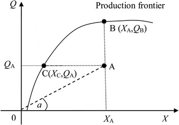
Let X ≡ X (x) and Q ≡ Q (q) denote the scalar aggregate output and input using a particular appropriate aggregator function. The production technology in equation (1) can be depicted by a frontier in an aggregate input and output space as shown in figure 1. The solid curve refers to the production frontier and point A is any observed data point. The dotted line connects the origin with point A with the angle of a. The productive scale of point A can be graphically quantified as tan a which equals to the ratio of Q A (observed aggregate output of A) to X A (observed aggregate input level of A). There are two important notes regarding this definition of productive scale. First, this definition of scale is identical to the scale and productivity concept which has received intensive discussions in the efficiency and productivity literature (Banker et al., Reference Banker, Cooper, Seiford, Thrall and Zhu2004; Khodabakhshi, Reference Khodabakhshi2009; O'Donnell, Reference O'Donnell2010). Second, the scale of any observed firm is not necessary ‘desirable’. For example, in figure 1, point A is not as desirable as point B because point B generates higher output using the same input level as point A. Similarly, point A is not as desirable as point C because point C uses less input but produces the same output level as point A.
Scale in aggregate input and output space

The prices of inputs and outputs can be incorporated in the aggregate input and output space by using the aggregate prices of the aggregate input and output, which can be calculated as:
 $$W = {\bf w}^{\prime} {\bf x}/X$$
 $$P = {\bf p}^{\prime} {\bf q}/Q.$$
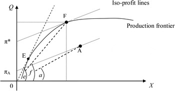
Figure 2 is an extension of figure 1 with the incorporation of the aggregate input and output prices. Any iso-profit line contains all feasible input-output combinations that have the same profit level (i.e., the same intersection between the iso-profit line and the vertical axis). The slope of many iso-profit lines is equal to the ratio of aggregate input price to aggregate output price (i.e., W/P). There exists only one point (i.e., point F) where the iso-profit line is tangent to the production frontier. Point F has a higher profit than any points on and below the production frontier. The scale at point F is called a profit-maximizing or an economically optimal scale. Guided by monetary gains, firms will often maximize their profits by moving to point F.
Profit-maximizing scale

Additionally, figure 2 shows point E at the tangency of the line passing through the origin and the production frontier. Point E has zero profit but generates the biggest angle (e), which is larger than f and a. Point E indicates the largest possible scale of production given the technology in equation (1). This figure also demonstrates that point F does not coincide with point E. Point F merges with point E if the iso-profit line has the same slope as the dashed line passing through the origin and point E. However, if this happens, the profit is zero (for example in central planning markets, all firms might have zero profits).
2.2. The materials balance principle and environmental efficiency
The first law of thermodynamics has been used to explain the relationship between economic activities and the environment since the late 1970s.Footnote 1 When being applied to the flows of materials, the MBP stipulates that materials in production systems are not lost and materials in inputs end up in either stock accumulation or desirable outputs. The stock accumulation can be undesirable because it contains the potential power to pollute the environment. Hence, the balance of materials can represent polluting emission. The MBP defines the MB u as:
 $$u = {\bf a}^{\prime}{\bf x} - {\bf b}^{\prime} {\bf q}$$
where non-negative vectors a and b represent the materials contents of inputs and outputs.
It is possible that several inputs such as labour and machinery could have zero contents of materials, which suggests that vectors a and b may include zero values (Coelli et al., Reference Coelli, Lauwers and Van Huylenbroeck2007; Hoang and Coelli, Reference Hoang and Coelli2011). The MBP applies to the flows of an individual material. In situations where there are many types of materials involved it is possible to use weights that reflect the polluting power of different materials in calculating the aggregate materials balance (Hoang and Coelli, Reference Hoang and Coelli2011). For example, N and P are two main nutrients that cause eutrophication problems in water systems. Analysis of eutrophication needs to use a particular set of weights that reflect the relative polluting powers of N and P. Systems like lakes and rivers tend to be limited more by P than N, and the over-enrichment of P results in a more damaging effect than the over-enrichment of N. In contrast, N is more commonly the key limiting nutrient of marine waters; thus, N levels have a greater polluting power in salt water systems than P. Hence, it is important that weights for N and P should be carefully determined in the context of specific systems so that their aggregate effects can be analyzed in empirical studies. Given appropriate N:P weights, the aggregate materials balance can be calculated.
Recently, researchers have advocated using the MPB to derive EE (Coelli et al., Reference Coelli, Lauwers and Van Huylenbroeck2007; Lauwers, Reference Lauwers2009). These studies seek feasible combinations of inputs and outputs to minimize the MB u in (5). There are three main approaches to solving this optimization problem. First, u can be minimized by contracting a′x given fixed outputs. Second, u can be minimized by expanding b′q given fixed outputs. Finally, u can be minimized by contracting a′x and expanding b′q. Several empirical studies have taken the first approach (Reinhard and Thijssen, Reference Reinhard and Thijssen2000; Coelli et al., Reference Coelli, Lauwers and Van Huylenbroeck2007; Welch and Barnum, Reference Welch and Barnum2009; Hoang and Coelli, Reference Hoang and Coelli2011).
2.3. Exergy, cumulative exergy and the ecological efficiency
The second law of thermodynamics stipulates that entropy, as the measure of usefulness of a closed system or a matter, tends to increase to a maximum level. Under this law, production activities are viewed as entropic; that transforms different materials and energy forms from low to high entropy matters. The matter with high entropy contains less usefulness.
The second thermodynamic law has several important applications in system analysis. First, both materials and energy contents can be converted to exergy, making the material inputs and energy inputs become comparable by using their respective exergy contents. Exergy contents (unit: joules) in mass and energy forms can be quantified as the maximum amount of work which can be produced by a system or a flow of mass/energy as it comes to equilibrium with a reference environment. Technical discussions on this quantification are described widely in the literature (Wall, Reference Wall1977; Szargut et al., Reference Szargut, Morris and Steward1988). Using exergy contents, the usefulness of all kinds of physical production inputs (i.e., human labour, animals, man-made capital, any forms of energy and any forms of materials and all ecosystem resources and services) can be incorporated into efficiency analysis (Hoang and Alauddin, Reference Hoang and Alauddin2011). Second, the second law of thermodynamics regulates the destruction of exergy. The amount of exergy destroyed indicates the consumption of resources as well as the power of degrading the quality of resources. This is a critical difference between the first and second law of thermodynamics. The first law regulates the conservations of mass and energy while the second law implies the actual consumption (destruction) of exergy (usefulness). Third, the concepts of life cycle assessment (LCA) can be captured by cumulative exergy consumption (CExC) analysis which extends exergy analysis beyond a single process to consider all processes from natural resources to the final products (even to the disposal of these products after being used) (Sciubba, Reference Sciubba2003). Recent research has developed rules to account for indirect (cumulative) exergy contents of non-physical inputs such as human services and monetary capital (Sciubba, Reference Sciubba2001). Formally, the CExC was defined as:
 $$z = {\bf c}^\prime {\bf x} - {\bf d}^\prime {\bf q}$$
where c is a strictly positive vector of the cumulative exergy contents of inputs and d a vector of the exergy contents of outputs. The cumulative exergy contents refer to total destruction of exergy (per unit of inputs) in all phases of manufacturing and disposing inputs. Additional exergy destruction involved in consuming or disposing of outputs can be captured by including an extra term in the vector q with a corresponding unit amount of exergy required to consume or dispose of the outputs.
Hoang and Rao (Reference Hoang and Rao2010) provide the first study that connects exergy analysis with efficiency measurement by solving feasible combinations of inputs and outputs to minimize the balance z in (6). The authors propose three optimization strategies: (i) maximize c′x given fixed d′q, (ii) maximize d′q given fixed c′x, and (ii) contract c′x and expand d′q simultaneously. Hoang and Rao (Reference Hoang and Rao2010) also supply an empirical application of the first optimizing strategy in the agricultural sector.
3. A framework of analyzing optimal scales from economic, environmental and ecological sustainability perspectives
3.1. Sustainable production and production economics
Different approaches to sustainable production use different methodologies and assign different significance to various aspects of sustainable production (Hansen, Reference Hansen1996; Glavic and Lukman, Reference Glavic and Lukman2007). Two frequently cited definitions of sustainable production in industrial and agricultural sectors read:
Sustainable production is creating goods by using processes and systems that are non-polluting, that conserve energy and natural resources in economically viable, safe and healthy ways for employees, communities, and consumers and which are socially and creatively rewarding for all stakeholders for the short- and long-term future. (Cited in Glavic and Lukman, Reference Glavic and Lukman2007: 1884)
A sustainable agriculture is one that, over the long term, enhances environmental quality and resource base on which the agriculture depends, provides for human fibre and food needs, is economically viable, and enhances the quality of life for farmers and society as a whole. (Cited in Hansen, Reference Hansen1996: 118)
Operationalizing the concepts of sustainability into empirical economic analysis is always a challenge. Analytical approaches to sustainable production frame three crucial dimensions of production activities: economic, environmental and ecological sustainability. The economic sustainability determines the sustained existence of the current market-based structure of human society. Firms, as economic agents in the market, pursue their primary objective of gaining economic returns which can be measured by monetary gains. The sustainability of money exchange between production and consumption depends critically on the firms' profitability. Therefore, it is reasonable to assume that firms tend to operate up to the scale at which their profits are maximized.Footnote 2
An outstanding concern of environmental economic analysis is how to minimize pollution caused by production. In this article, the environmental perspective of sustainable production is limited to the issue of minimizing pollution. In many such situations the polluting effects of production, as regulated by the first law of thermodynamics, can be represented by the balance of materials; hence, the environmental objective of sustainable production is to minimize the materials balance. However, from an ecological point of view, sustainable production is not only concerned with the environmental effects of production, but also the sustained availability and quality of the natural resources and the services of the ecosystem. The ecological perspective of sustainable production is to seek the optimal production scales at which the total extraction of the ecosystem services and resources, as well as the cumulative effects of pollution, can be minimized. Practically, the balance of cumulative exergy can represent the total resource extraction and cumulative pollution; therefore, the ecological objective of sustainability is to minimize this balance.
In pursuing profit-maximizing objectives, past and current production practices have been unsustainable in terms of environmental and ecological considerations (Brundtland, Reference Brundtland1987). This occurred as a result of the failures of past and existing market structures (even with governmental interventions) to account properly for the externalities of production and related ecosystem services and resources. The environmental pollution and the degradation of the ecosystem resources and services, in the long run, will limit the growth of economic activities. This suggests that given market failures, economically sustainable production does not warrant environmental and ecological sustainability. The following sections develop a framework in which optimal scales from these three perspectives of sustainable production can be analyzed simultaneously.
In sum, sustainable production is a very broad concept and covers many interrelated dimensions. For the sake of simplicity, economic, environmental and ecological perspectives to sustainable production used in the present article have fine (even narrow) definitions: they are related to the maximization of profits and minimizations of materials and cumulative exergy balances, respectively. These simplified interpretations, however, are very helpful in the construction of a simple analytical framework that empirical analysts can use.
3.2. Optimal scales
The economic, environmental and ecological optimization problems in equations (2), (5) and (6) can be rewritten as:
 $$\hbox{maximize } \pi = {\bf p}^\prime {\bf q} - {\bf w}^\prime {\bf x} = PQ - WX$$
 $$\eqalign{\hbox{minimize u} & = {\bf a}^\prime{\bf x} - {\bf b}^\prime{\bf q} = \hbox{AX} - \hbox{BQ} \hbox{ or maximize } {-} \hbox{u} \cr & = {\bf b}^\prime{\bf q} - {\bf a}^\prime{\bf x} = \hbox{BQ} - \hbox{AX}}$$
 $$\eqalign{\hbox{minimize z} & = {\bf c}^\prime{\bf x} - {\bf d}^\prime{\bf q} = \hbox{CX} - \hbox{DQ} \hbox{ or maximize } {-} \hbox{z} \cr & = {\bf d}^\prime{\bf q} - {\bf c}^\prime{\bf x} = \hbox{DQ} - \hbox{CX}}$$
where P and W have been defined in equations (3) and (4). B and D are aggregate materials and exergy contents of the aggregate output, while A and C are the materials and cumulative exergy contents of the aggregate input. These aggregate terms can be calculated as:
 $$A = {{\bf a}^\prime {\bf x}\over{X}}$$
 $$B = {{\bf b}^\prime {\bf q}\over{Q}}$$
 $$C = {{\bf c}^\prime {\bf x}\over{X}}$$
 $$D = {{\bf d}^\prime {\bf q}\over{Q}}.$$
Note that the objective functions in equations (7)–(9) are similar in the mathematical formats and that they all contain the same inputs and outputs of the production technology in equation (1). The only difference rests in the pairs of the vectors of (a and b), (c and d) and (p and w). This implies that both parametric and non-parametric methods can be used in a similar manner to solve these optimization problems. Rewrite equations (7)–(9) as:
 $$Q = {\pi \over P} + {W \over P} X$$
 $$Q = -{u \over B} + {A \over B} X$$
 $$Q = -{z \over D} + {C \over D} X.$$
Equations (15) and (16) suggest that, when the information of nutrient contents (a and b) and cumulative exergy contents (c and d) of the input and output vectors is available, we can construct aggregate nutrient and exergy contents (A, B, C and D) and use them in the aggregate input and output space. The information of A, B, C and D can be used to construct iso-material balance and iso-exergy balance lines. The incorporation of the iso-material balance and iso-exergy balance lines into the aggregate input and output space is analogous to the previous discussion of the iso-profit lines.
Figure A1 in the online appendix available at http://journals.cambridge.org/EDE presents the concept of iso-material balance lines passing through points A, E and G. Point A representing any observed data point and point E generating the maximum TFP level have been already mentioned in figure 2. Point G is at the tangency of the iso-material balance line and the production frontier. There are two important observations: first, the intercepts of all iso-material balance lines are negative because the MBP regulates that −u is strictly negative (because u is strictly positive) and second, point G has the minimum balance of materials, suggesting that point G represents the environmentally optimal scale.
Figure A2 (online appendix) graphs iso-exergy balance lines for points A, C and H. Point H is where the iso-exergy balance line is tangent to the unrestricted frontier, yielding the smallest exergy balance for all possible firms. From the ecological perspective, point H is the most sustainable because it causes the smallest amount of pollution and consumes the smallest amount of natural resources.
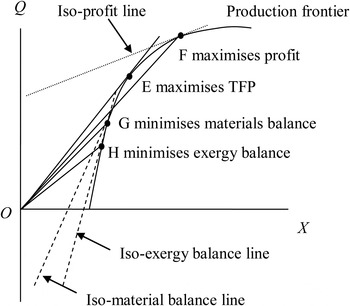
Figure 3 presents all optimal scales from economic, environmental and ecological sustainability perspectives. Point F maximizes the profit and this is the target for firms in the profit-driven markets. Point E maximizes the TFP levels and this point is the most desirable point by economic planners. Point G is of special interest in terms of environmental pollution because it minimizes the balance of materials, which causes pollution. Point H minimizes the cumulative exergy balance. Since the cumulative exergy balance has two aspects: cumulative pollution and total extraction of resources, point H has received special attention from the perspective of ecological sustainability.
Different scales under different sustainable objectives

In this hypothetical situation, all of these points do not coincide. Graphically, holding constant the non-decreasing-return-to-scale aggregate production frontier, the ranking of points F, G, and H is determined by two factors: (1) the ordering of the slope (i.e., W/P < A/B < C/D derived from equations (14)–(16); and (2) the ordering of intercept values on the Q-axis of the iso-profit, iso-material balance and iso-exergy balance lines (πmax/P,-umax/B, - zmax/D where subscript max refers to the maximum absolute values of profits, MB and exergy balance). πmax/P predicted to be positive in this diagram captures situations where there are profitable farms in the industry. The first and second laws of thermodynamics demand that -umax/B and -zmax/D are strictly negative; hence the intercepts of the iso-exergy balance and exergy line stay below the origin. The presence of life cycle effects in the calculation of exergy balance (but not in the calculation of MB) results in the intercept of the iso-exergy balance line staying below the intercept of the iso-material balance line.
Note that changes in the prices of inputs and outputs will change the iso-profit line and can merge this line with the OE, iso-material and iso-exergy balance lines. Points E and F become one when the iso-profit line becomes the OE line, which means that the profit at this point is zero. Similarly, point F can come to point G where the profit equates BQ-AX, which is negative because AX- BQ is strictly positive. In the same logic, point F can come to point H where the profit equates DQ-CX, which is negative because the exergy balance (i.e., CX- DQ) is strictly positive. These analyses imply that there exist ‘natural’ trade-offs between profit and environmental (ecological) considerations. Given the fact that firms will operate at scales that are not optimal for the natural environment, the economic approach to sustainable development is to intervene by imposing policies in order to change a firm's behaviour. One obvious possibility is to affect the markets of inputs and outputs so that firms will reduce their production scale; however, simply changing input and output prices may cause huge financial loss to firms, which will not make firms economically sustainable. Hence, there is a demand for a more sophisticated approach to policy interventions. A more holistic approach to policy intervention should focus on the minimization of exergy destruction during the life cycle process of production and consumption. Policies that improve energy efficiency, minimize waste in production and consumption, promote technological innovations, and even reduce consumption demands for goods and services are all relevant and need further examination.
This proposed framework delivers a useful tool for empirical studies. For example, using policies to affect input and output prices raises a question: how much does it cost to move firms from economically optimal scales to environmentally and ecologically optimal scales. This question can be presented by movements of point F to points G and H. To address this question in empirical analyses, the following steps must be addressed: (1) data on prices, nutrients and exergy contents of inputs and outputs need to be available in order to identify these points (E, F, G and H); (2) at these points, TFP, profit, materials balance, exergy balance can be calculated; (3) the differences between the maximum profit (the profit of point F) with any profit at any other points (i.e., G or H) can be used as the estimates of costs to move them from point F to the corresponding point. For example, if the policy makers are to estimate how much it costs to move firms from point F to point G to minimize the pollution, the difference in the profits of these two points can be used as the estimated cost.
The proposed framework also facilitates the development of new EE and productivity measures. Figure A3 (online appendix) illustrates that points G and H should be the target for all firms to move towards so that their production activities have the smallest negative impact on the surrounding environment. This means that in measuring environmental and ecological efficiency, the performance of any individual firm should be evaluated against these targets. One may wish to benchmark point A against points G (or H) via points B1, B2 or B3. The distance from point A to point B1 measures an input-orientated TE, while the distance from point B1 to point G (or H) can be defined as the environmental (or ecological) allocative efficiency. Under the output orientation, point A can be assessed against point B2 then to point G (or H); hence, |AB2| denotes an output-orientated TE, while |B2H| (or |B2G |) measures the environmental (or ecologically) allocative efficiency. Alternatively, one can use the directional distance functions (DDFs) to evaluate point A to point B3 then to point G (or H).
Note that the uses of (input, output and directional) distance functions in the present paper differ from other proposals in the literature in two ways. First, in this paper distance functions are used in the aggregate input and output space which can also facilitate the analysis of economies of scope. Secondly, modelling pollution or total cumulative destruction of ecosystem resources in this framework is consistent with the MBP. As shown elsewhere (Hoang and Coelli, Reference Hoang and Coelli2011; Hoang and Alauddin, Reference Hoang and Alauddin2012; Hoang and Nguyen, Reference Hoang and Nguyen2013), those models that include nutrients balance (and exergy balance) as either extra outputs or inputs in the production functions will not conform to the first and second laws of thermodynamics.
4. An empirical illustration
4.1. Data description and estimation techniques
The present article utilized a data set of 88 rice farms in Gangwon province of South Korea from 2003 to 2007. The data were taken from the Agricultural and Livestock Production Cost Survey of the Microdata Service System of the Korean National Statistical Office. This data set is a balanced panel of a bigger data set, a detailed description of which appears in Nguyen et al. (Reference Nguyen, Hoang and Seo2012).
There are one major output (i.e., net quantity of rice grain) and six major inputs including land (measured in ha), labour (working hours of family and hired labour), organic fertilizers (total amount of active nitrogen (N), phosphorous (P) and potash (K)), inorganic fertilizers (total amount of active N, P, and K), pesticides (total amount of active fungicides, herbicides and insecticides) and energy (total quantity of lime, diesel, gasoline, kerosene and electricity).
In terms of the environmental pollution of rice production on water systems, N and P are considered to have the most damaging impacts in Korea (Kim et al., Reference Kim, Park, Hwang and Choi1997). We followed previous studies (Hoang and Alauddin, Reference Hoang and Alauddin2012; Nguyen et al., Reference Nguyen, Hoang and Seo2012) to use a set of weights (1N:10P suggesting P is considered to be 10 times more damaging than N) in our analysis. The N and P contents of rice paddy were assumed to be 0.015 kg N/kg and 0.0027 kg P/kg (FAO, 1972); hence the aggregate nutrient content of rice paddy was 0.042 (i.e., 0.015 + 10 * 0.0027). The nutrient contents of labour, pesticides (from three main groups of products: fungicides, insecticides and herbicides) and energy (five main types: lime, diesel, gasoline, kerosene and electricity) were assumed to be zero. The aggregate nutrient amounts in organic and inorganic fertilizers are the sum of N and P adjusted with the chosen weight set. The nutrient content of land was calculated as in Nguyen et al. (Reference Nguyen, Hoang and Seo2012).
We used data on chemical exergy contents and cumulative exergy consumption for the manufacturing, packaging and transportation of relevant inputs. Particularly, we used the total energy consumption in the manufacturing, packaging and transportation of various types of pesticides and inorganic fertilizers reported in the literature (Green, Reference Green and Helsel1987; Bhat et al., Reference Bhat, English, Turhollow and Nyangito1994). The exergy contents of organic fertilizers were assumed to be 303 kJ/kg (Hatirli et al., Reference Hatirli, Ozkan and Fert2006). Data on the chemical exergy content of lime, diesel, gasoline, kerosene and electricity were from various sources (Dincer and Rosen, Reference Dincer, Rosen and Paksoy2007). Data on energy contained in the food consumption reported by Food and Agriculture Organization (FAO) for Korea was used to capture the exergy contribution of labour (i.e., 530 kJ/hour) (Hoang and Alauddin, Reference Hoang and Alauddin2011). The exergy content of land was assumed to be the amount of chemical exergy contained in organic matter lost in topsoil (i.e., 172,000 kJ/ha) (NEAD, 2009). The metabolizable energy of rice paddy (i.e., the output) was assumed to be 14.3 kJ/kg (FAO, 1972). Descriptive statistics are shown in table A1 (online appendix).
DEA was used to aggregate six inputs into one single aggregate input term (X) using the Malmquist input distance function. DEA does not take into account the data noise and solves for local solutions; hence its interpretations require caution.Footnote 3 The aggregate price (W), nutrient content (A) and exergy content (C) of the aggregate inputs were derived implicitly (e.g., W = w′x/ X , A = a′x/ X and C = c′ x/ X ). Once the aggregate input was constructed, the optimization problems in equations (1)–(9) become situations with only one output and the single aggregate input. Another set of input-orientated DEA problems were solved to estimate the aggregate production frontier Y = f(X) as shown in figure 2.
Since the data set does not cover the entire population of rice farms in Korea, bootstrap DEA was used to remove sample bias with 2,000 replications (Simar and Wilson, Reference Simar and Wilson1998). The average scores estimated from standard DEA and bootstrap DEA models are in table A2 (online appendix). Both the constant returns to scale (CRS) and variable returns to scale (VRS) specifications of the production technology were estimated using the input orientation framework. As shown in table A3 (online appendix), the results of bootstrap tests prefer the CRS specification; hence the results under the CRS technology are presented in the next section.
4.2. Results
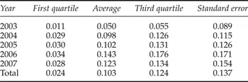
Table 1 reports the average values of TE in the CRS specification. On average, farms were estimated to be 10.3 per cent efficient in relation to the CRS frontier, suggesting that they could reduce the consumption of the aggregate input by 89.7 per cent without any reductions in the output level. The majority of farms (75 per cent) have annual average efficiency levels of lower than 13 per cent. The efficiency scores varied greatly across 88 farms, which warrant further investigations into finding the determinants of efficiency performance.
Summary of technical efficiency scores

DEA results also allow one to identify an ‘efficient’ position projected on the estimated frontier for any individual farm in a single year. Figure A4 (online appendix) presented an illustration for year 2003 where the efficient position for a typical farm was projected on the frontier.Footnote 4 This ‘efficient’ position suggested that the level of the aggregate input could be just 0.063 in comparison to the currently used level of 1.053, which suggests that this farm can achieve significant reductions in production costs and the consumption of nutrients and exergy.
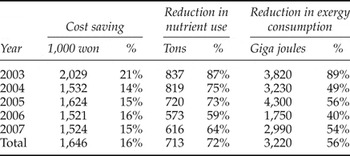
Given the existing ‘average’ price, nutrient and exergy information of the aggregate input and output, table 2 reported the ‘average’ magnitude of reductions in production costs and the consumption of nutrients and exergy. The results showed that the ‘average’ farm could increase its profit by more than 16 per cent (due to reduction in production costs) while the balance of nutrient (1N:10P) and exergy could be reduced by nearly 72 per cent and 56 per cent, respectively. This finding suggests that there is not always a trade-off between economic, environmental and ecological performance for most farms: being more efficient in using inputs could help farms achieve higher economic returns and at the same time reduce impacts caused on the surrounding water systems and entire ecosystem.
Potential economic, environmental and ecological improvements for the ‘average’ farm overtime

Results in table 2 also showed some evidence of an increasing trend of TE over time. Figure A5 (online appendix) presenting kernel density estimates of TE scores in five periods show that the shape of TE distribution also varied from one year to another, suggesting distribution dynamics of efficiency scores over time. In order to investigate intra-distribution dynamic movements of individual farms in relation to the frontier, we estimated stochastic kernels for one-year and five-year transitions using mean-corrected efficiency scores. In the one-year transitions as shown in figure A6 (online appendix), the kernel density of TE scores in one period (i.e., t + 1) is conditional on that of the TE scores in a previous period (period t).Footnote 5 The contour plots suggest that a probability mass concentrated along the positive sloped diagonal, which infer that inter-annual mobility of farms is not very high and there is persistence in the efficiency relative to positions of farms. Transitions from year 2003 to 2007 as in figure A7 (online appendix) show that intra-distribution mobility is higher. In particular, probability seems to concentrate in three regions of which two less concentrated groups represent highly efficient farms. The most concentrated region shows that probability seems to concentrate horizontally at about 1–4 in 2007, suggesting that the initial relative positions in 2003 are more dispersed than relative positions in 2007 and that there is higher mobility of positions relative to frontiers of farms in this group.
5. Conclusion
A simple analytical framework was proposed in this paper to translate the concepts of sustainable production to three simplified dimensions of economic, environmental and ecological sustainability. In this framework optimal production scales can be identified by solving three optimizing problems in the aggregate input and output space. First, economic optimizations seek combinations of inputs and outputs to maximize profits. Second, environmental optimizations search for input-output combinations that minimize the polluting effects of materials balance on the surrounding physical environment. Third, ecological optimizations look for input-output combinations that minimize the total and cumulative destruction of the entire ecosystem (i.e., cumulative exergy balance). The simplification of sustainability concepts was done in favour of simple and practical applicability of the proposed framework.
The use of the aggregate input and output quantity space helps provide diagrammatical analysis of optimal scales from the three perspectives of sustainable production in relation to the concepts of efficiency and productivity commonly used in empirical studies. The theoretical analysis showed that firms motivated by profit gains would operate at the scale which is larger than optimal scales from the ‘simplified’ perspectives of environmental and ecological sustainability. For a typical firm which lies under the frontier, this tendency is due to the failure of input and output markets to account properly for the negative effects of production on the surrounding environment and the whole ecosystem. Efficient firms which lie on the frontier face trade-offs between profit-maximizing and environmental/ecological considerations, sending evidence to favour policy interventions.
An empirical application using a data set of Korean rice farms yielded several important findings. First, farms could have achieved higher profit in conjunction with a smaller amount of nutrient released into the surrounding system and a smaller amount of exergy destruction by being more efficient in using inputs (i.e., moving towards the aggregate production frontier). Second, the scales at which farms were to maximize their profits were estimated to be higher than sales at which the balances of nutrient and exergy were to be minimized, implying a trade-off for technically efficient farms (i.e., staying on the frontier) between economic returns and objectives of minimizing the environment/ecological impacts of their production. Third, there was low mobility of farms in their positions relative to the frontier from one year to another year, which suggests that the majority of farms failed to achieve improvement in their efficiency positions over the five-year period surveyed.
There are several important directions for future research. First is the modification of the proposed framework using the actual disaggregated multiple input and output space to avoid possible loss of information during aggregation procedures. Second, the proposed framework pays attention to negative externalities of production while production activities may exhibit positive externalities; hence the latter should be modelled to provide more comprehensive analyses. Third, it is important to apply this framework in empirical situations where market failures exist. Such empirical studies would provide a new method of valuating the environmental and ecological costs of production externalities in which monetary valuation of externalities could be benchmarked against actual pollution caused to the surrounding environment and ecosystem.
Supplementary materials and methods
The supplementary material referred to in this paper can be found online at journals.cambridge.org/EDE/.