1. Introduction
Screw theory is a powerful mathematical tool that plays a key role in the field of mechanical engineering, especially in mechanisms and robotics. It uniformly describes the screw, rotational, and translational motions of a rigid body and has the advantages of clear geometric meaning, concise expression form, and convenient algebraic operations. It can concisely reveal the relationship among the velocity models of robotic mechanisms and the relationship between the force and motion of a rigid body under the action of a spatial force system. Therefore, it is widely applied in fields such as serial robots [Reference Hunt, Samuel and McAree1–Reference Song, Liu, Lian, Qi, Wang, Wu and Li3], parallel robots [Reference Wang, Qiu, He, Wu, Xu and Zhao4–Reference Wang, Xiong, Zhang and Yuan6], and deployable mechanisms [Reference Shen and Yang7, Reference Huang, Zhang, Xiong and Liu8].
In robotics, there are two kinds of screws including instantaneous screw and finite displacement screw. The former focuses on the instantaneous motion characteristics of a mechanism and is often used to analyse the instantaneous property of a mechanism, such as the instantaneous degrees of freedom (DOF). For example, Huang [Reference Huang, Xia and Ding9] calculated the DOF of the Bennett mechanism by using screw theory and realized the application of screw theory in the calculation of the DOF of closed-loop mechanisms. Dai et al. [Reference Dai, Huang and Lipkin10] proposed a method for calculating the DOF of parallel robots based on screw theory, solving the problem of incorrect calculation results caused by redundant DOF when using the traditional G-K formula to calculate the DOF of parallel robots. Sun et al. [Reference Sun11] proposed a concise method for calculating the DOF of terminal link about a serial robot based on screw theory and the kinematic output matrix. Cao et al. [Reference Cao, Xi, Ding and Chen12] proposed a novel double-ring truss deployable satellite antenna mechanism and obtained its correct DOF using screw theory. Zou et al. [Reference Zou, Zhang, Zhang, Zhang, Wu and Qin13] proposed a 3-RRS (R for rotational joint, S for spherical joint) parallel ankle rehabilitation robot, and used screw theory to analyse its DOF and kinematics.
The finite displacement screw describes the finite displacement of a rigid body within a certain range as a mathematical tool. It uses a finite screw to describe the motion and force transmission of a rigid body, can analyse the kinematic and dynamic characteristics of a mechanism concisely and effectively. It is often used to analyse the overall DOF of a mechanism and can also be used to obtain the kinematic relationships between various motion angles in a mechanism. For example, as early as 1995, Dai et al. [Reference Dai, Holland and Kerr14] applied the transformation and representation of finite screws to planar serial manipulators with revolute joints, thereby demonstrating the characteristics of their workspaces and clarifying the parametric representation of the joint space description of the manipulator. Yang et al. [Reference Yang and Li15] proposed a new type of deployable parallel mechanism on the basis of existing closed-loop deployable mechanisms and parallel mechanisms, and then, they calculated its DOF by using the finite screw theory and established its forward and inverse kinematic equations. Guo et al. [Reference Guo, Lian, Song, Qi and Sun16] established the motion closed-loop equation of the Myard mechanism using the finite screw theory, so as to solve the relationship between the various motion angles of the mechanism, and carried out kinematic analysis on the Myard annular networking mechanism. Liu et al. [Reference Liu, Lian and Li17] established the topological model and velocity model of the Exechon parallel robot by using the finite screw theory, and solved its DOF as well as the velocity and force Jacobian matrices, laying a foundation for the subsequent optimization of this parallel robot. Qi et al. [Reference Qi, Zhang, Ren, Tong, Liang and Han18] used the finite screw theory to solve the method for obtaining the explicit solution of the motion equation of the serial robot and described its finite motion.
The above applications are limited to linkage mechanisms that do not include higher pairs. However, higher pair mechanisms exhibit significant applications in particular areas because they can achieve complex motions with a more concise structure by reasonably designing contact contours. They are widely used in fields such as robotics [Reference Baek, Moon, Choi and Koo19–Reference Song, Fu, Romano, Dario and Kang21], automated equipment [Reference Jiang, Chen, Li, Ma, Ren and Mao22, Reference Xue, Ye and Hu23], and precision instruments [Reference Ming, Wang, Cai, Li, Wang, Jing and Zhou24]. For example, Kimura et al. [Reference Kimura, Iwatsuki and Ikeda25] proposed an “active” spatial rolling contact higher pair. It is driven by multiple active elastic elements to achieve a simple spatial path for the mechanism. In dentistry, lower-pair mechanisms composed of spherical pairs and revolute pairs have been proposed to simulate the occlusion of mandibular movement, but none of them can achieve the compound movement of bionic condyle. To address this problem, Wen [Reference Wen, Cong, Wang, Qin, Xu and Zhang26] proposed a redundantly actuated parallel robot that realizes mandibular movement by adding two point-contact constraints. Experiments have proven that this mechanism can not only simulate mandibular movement but also simulate chewing force and temporomandibular joint force. In high-voltage circuit detection, in order to achieve the detection task of high-voltage insulators, Yuan et al. [Reference Yuan, Yuan, Wang and Song27] proposed an insulator detection robot with a lightweight, compact structure and high adaptability based on higher kinematic pair (HKP) mechanisms. To solve the problem that traditional mechanical automatic machines are difficult to completely realize movement on a user-specified trajectory, Cheng et al. [Reference Cheng, Sun, Song and Liu28] proposed a method for establishing a new cam mechanism. The follower of this mechanism can accurately realize the user-specified trajectory, offering a new idea for the design of new robots. The curve-face gear mechanism is a novel type of mechanism that combines a cam mechanism and a gear mechanism. It has the characteristic of variable transmission ratio, and the kinematic pair between the two parts belongs to a HKP. To better describe the movement of this mechanism, Lin et al. [Reference Lin, Wei and Cai29], based on screw theory, regarded the point-contact higher pair between gears as helical motion, and thereby analyzed the meshing characteristics and motion laws of the curved surface gear compound transmission mechanism. But this application method of screw theory on HKP is only applicable to the motion analysis of mechanisms where the HKP trajectory is on a cylindrical surface.
Currently, the DOF calculation for existing HKP mechanisms primarily relies on the G-K formulas through a numerical counting approach. However, this method fails to adequately account for the kinematic dimensions of mechanisms, potentially introducing computational errors. Due to the absence of a unified and comprehensive method, researchers are often compelled to employ geometric approaches [Reference Song, Fu, Romano, Dario and Kang21, Reference Wen, Cong, Qin and Xu30] to discuss the motion characteristics of higher-pair mechanisms. Therefore, it is necessary to develop an approach suitable for all HKP mechanisms. Although screw theory has proven to be an efficient tool in the kinematics, its application remains predominantly confined to linkages comprising only with lower pairs. To enhance the adaptability of screw theory, this paper proposes an approach to extend instantaneous screw and finite displacement screw theories to mechanisms with higher kinematic pairs, enabling their kinematic analysis. This approach can not only analyse the instantaneous DOF of HKP mechanisms but also solve the relationship between the motion variables of HKP mechanisms. The layout of this paper is as follows. Section 2 analyzes the motion mode of HKPs, and then, presents a method for calculating the DOF of HKP mechanisms based on screw theory. The associated application of finite screw theory to HKP mechanisms is presented in Section 3. Section 4 exhibits the kinematic analysis of four classic higher pair mechanisms, including a planar, two spatial, and a hybrid one, to verify the practicability and accuracy of the proposed method. And conclusion in Section 5 ends the paper.
2. The instantaneous screw theory for analysing DOF of mechanisms with higher kinematic pairs
In screw theory, the motion screw system of each branch can be determined by establishing a global coordinate system, and the constraint screw system of each branch can be calculated by using the duality between the motion screw system and the constraint screw system. Through this approach, the constraint screw multiset of the platform can be obtained. Subsequently, the maximum linearly independent group can be calculated, and then the motion of the platform can be determined. According to screw theory, in a kinematic chain obtained by connecting n revolute joints in series, the instantaneous motion screw of the end rigid body can be expressed as:
 \begin{equation} \omega _{\mathrm{e}}\boldsymbol{\$}_{\mathrm{e}}=\omega _{1}\boldsymbol{\$} _{1}+\omega _{2}\boldsymbol{\$} _{2}+\omega _{3}\boldsymbol{\$} _{3}+\omega _{4}\boldsymbol{\$} _{4}+\ldots +\omega _{\mathrm{n}}\boldsymbol{\$} _{\mathrm{n}} \end{equation}
which
 $\omega _{e}$
is the angular velocity of the end rigid body,
 $\boldsymbol{\$} _{\mathrm{e}}$
is the screw of the end rigid body,
 $\omega _{i}$
is the angular velocity of the i-th axis, and
 $\boldsymbol{\$} _{\mathrm{i}}$
is the screw of the i-th kinematic pair. This equation is called the screw equation.
When this serial mechanism forms a closed loop, its end rigid body is the frame, and then its velocity relative to the reference configuration is 0. At this time, the screw equation of the mechanism can be written as [Reference Dai and Jones31]:
 \begin{equation} \omega _{1}\boldsymbol{\$} _{\boldsymbol{1}}+\omega _{2}\boldsymbol{\$} _{2}+\omega _{3}\boldsymbol{\$} _{3}+\omega _{4}\boldsymbol{\$} _{4}+\ldots +\omega _{\mathrm{n}}\boldsymbol{\$} _{\mathrm{n}}=\boldsymbol{0} \end{equation}
It can be written as,
 \begin{equation} \boldsymbol{M}\boldsymbol{\omega }=0 \end{equation}
where
 $\boldsymbol{M}=(\begin{array}{l@{\quad}l@{\quad}l@{\quad}l@{\quad}l@{\quad}l} \boldsymbol{\$} _{1} & \boldsymbol{\$} _{2} & \boldsymbol{\$} _{3} & \boldsymbol{\$} _{4} & \ldots & \boldsymbol{\$} _{\mathrm{n}} \end{array}), \boldsymbol{\omega }=(\begin{array}{l@{\quad}l@{\quad}l@{\quad}l@{\quad}l@{\quad}l} \omega _{1} & \omega _{2} & \omega _{3} & \omega _{4} & \ldots & \omega _{n} \end{array})^{\mathrm{T }}$
This closed-loop equation illustrates the relationship between each joint and the DOF of the mechanism. Analyzed from the perspective of linear algebra, the DOF of a mechanism depends on the difference between the total number of joints and the number of linearly independent joints, i.e., the DOF of the mechanism is equal to the dimension of the null space vector of matrix [Reference Wei, Ding and Dai32].
 \begin{equation} m=\text{nullity}(\boldsymbol{M})=n-\text{rank}(\boldsymbol{M}) \end{equation}
where
 $m$
is the DOF of the mechanism, and
 $n$
is the dimension of
 $\boldsymbol{\omega }$
.
 $\boldsymbol{M}$
is called the constraint matrix of this mechanism.
Since the screw theory can only be used to represent various lower kinematic pair mechanisms at present, the above method is only suitable for calculating the DOF of mechanisms with no HKPs. Next, the approach for calculating the DOF of HKP mechanisms by using screw theory is introduced.
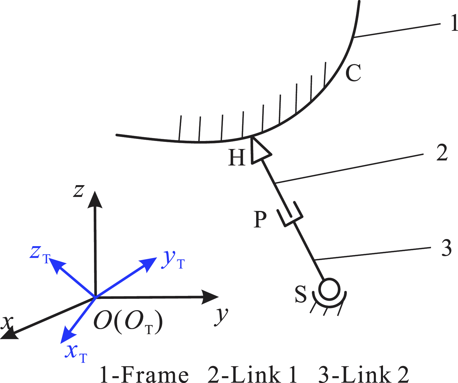
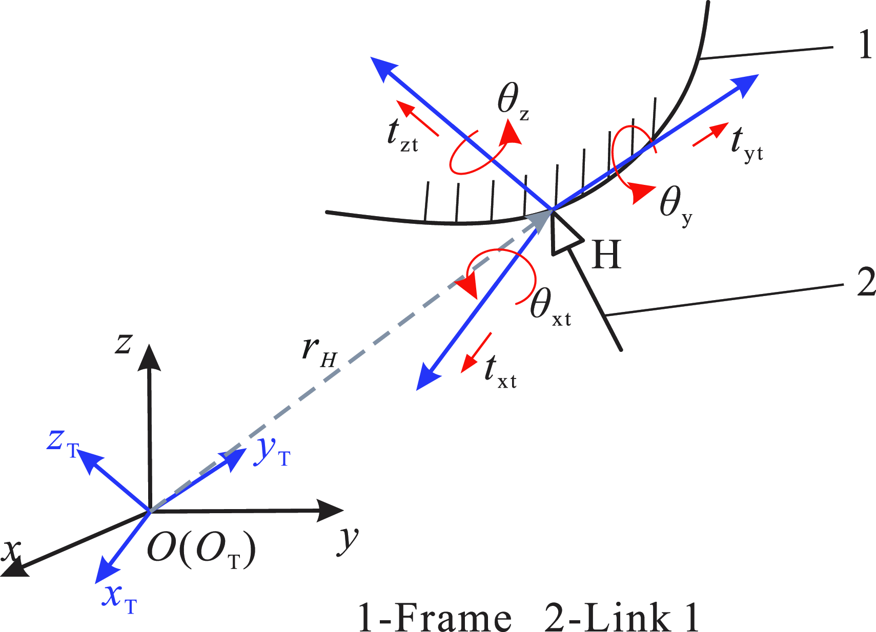
First, we will discuss how to represent the instantaneous screw of a high kinematic pair. A HKP is a kinematic pair formed by two components through point contact or line contact. Compared with the surface contact of a lower kinematic pair, it has fewer constraints and more DOFs. For an ordinary spatial HKP mechanism in Figure 1, which is composed of a spherical pair S, a prismatic pair P and a HKP H. The parametric equation of trajectory curve C under the trajectory coordinate system
 $O_{\mathrm{T}}-x_{\mathrm{T}}y_{\mathrm{T}}z_{\mathrm{T}}$
is
 $\left\{\begin{array}{c} x=x\left(t\right)\\ y=y\left(t\right)\\ z=z\left(t\right) \end{array}\right.,t\in R$
. The frame and link 1 form a HKP, and the contact point between them is point H.
A spatial higher kinematic pair mechanism.

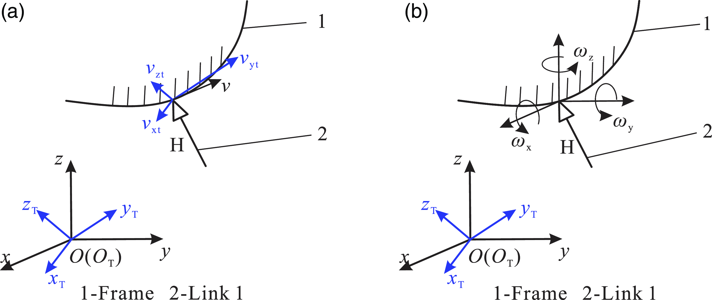
In kinematics of mechanisms, it is well known that the addition of a new kinematic pair will result in the additional constraint. Once two components are joined by means of a high kinematic pair, at the contact point or along the contact line, the relative motion in the direction of the contact normal is effectively constrained. Nevertheless, there remains the potential for relative motion between the two components sliding along the direction of the contact tangent as well as around the contact point in terms of rotation. Therefore, in order to better describe the expression of the instantaneous screw of the HKP, we decompose the motion of the HKP. In the Figure 1, in the case of considering only the constraint of HKP H, we divide the motion of link 1 into two parts as shown in Figure 2. The first one, see Figure 2(a), is the sliding of point H on link 1 along trajectory curve C, and the second one, see Figure 2(b), is the rotation of link 1 around contact point H.
The motion decomposition of the higher kinematic pair. (a) The sliding in the higher kinematic pair. (b) The rotation in the higher kinematic pair.

As shown in the Figure 2(a), the sliding velocity
v
of the contact point H on the trajectory curve C will always be along the tangent direction of curve, and it can be decomposed into velocity components
 $\boldsymbol{v}_{\mathrm{xt}}, \boldsymbol{v}_{\mathrm{yt}}$
, and
 $\boldsymbol{v}_{\mathrm{zt}}$
along the three directions of the
 $O_{\mathrm{T}}-x_{\mathrm{T}}y_{\mathrm{T}}z_{\mathrm{T}}$
. Therefore, this motion can be regarded as being composed of three prismatic pairs. Since the point H always moves along the trajectory, there is a certain relationship among
 $\boldsymbol{v}_{\mathrm{xt}}, \boldsymbol{v}_{\mathrm{yt}}$
and
 $\boldsymbol{v}_{\mathrm{zt}}$
, it can be obtained from the parametric equation of the trajectory curve C, i.e.,
 \begin{equation} \begin{array}{c} R_{\mathrm{a}}=\dfrac{\boldsymbol{v}_{\mathrm{yt}}}{\boldsymbol{v}_{\mathrm{xt}}}=\dfrac{dy}{dx}=\dfrac{dy/dt}{dx/dt}\\[10pt] R_{\mathrm{b}}=\dfrac{\boldsymbol{v}_{\mathrm{zt}}}{\boldsymbol{v}_{\mathrm{xt}}}=\dfrac{dz}{dx}=\dfrac{dz/dt}{dx/dt} \end{array} \end{equation}
where
 $R_{\mathrm{a}}$
and
 $R_{\mathrm{b}}$
are proportional relationship between
 $\boldsymbol{v}_{\mathrm{yt}}$
and
 $\boldsymbol{v}_{\mathrm{xt}}$
, and the proportional relationship between
 $\boldsymbol{v}_{\mathrm{zt}}$
and
 $\boldsymbol{v}_{\mathrm{xt}}$
, respectively. The relationship can be rewritten as,
 \begin{equation} \begin{array}{c} R_{\mathrm{a}}\boldsymbol{v}_{\mathrm{xt}}-\boldsymbol{v}_{\mathrm{yt}}=0\\ R_{b}\boldsymbol{v}_{\mathrm{xt}}-\boldsymbol{v}_{\mathrm{zt}}=0 \end{array} \end{equation}
Therefore, this part is composed of three coupled prismatic pairs. According to the screw theory, the instantaneous screw of sliding part can be written as,
 \begin{equation} \left\{\begin{array}{c} \textit{v}_{\mathrm{xt}}\boldsymbol{\$} _{\mathrm{xt}}=\textit{v}_{\mathrm{xt}}\left(\begin{array}{c} \boldsymbol{0}\\ \boldsymbol{s}_{\mathrm{xt}} \end{array}\right)\\[10pt] \textit{v}_{\mathrm{yt}}\boldsymbol{\$} _{\mathrm{yt}}=\textit{v}_{\mathrm{yt}}\left(\begin{array}{c} \boldsymbol{0}\\ \boldsymbol{s}_{\mathrm{yt}} \end{array}\right)\\[10pt] \textit{v}_{\mathrm{zt}}\boldsymbol{\$} _{\mathrm{zt}}=\textit{v}_{\mathrm{zt}}\left(\begin{array}{c} \boldsymbol{0}\\ \boldsymbol{s}_{\mathrm{zt}} \end{array}\right) \end{array}\right. \end{equation}
where
 $\textit{v}_{\mathrm{xt}}\boldsymbol{\$} _{\mathrm{xt}}, \textit{v}_{\mathrm{yt}}\boldsymbol{\$} _{\mathrm{yt}}$
, and
 $\textit{v}_{\mathrm{zt}}\boldsymbol{\$} _{\mathrm{zt}}$
respectively represent the instantaneous screws for sliding along the three directions of the
 $O_{\mathrm{T}}-x_{\mathrm{T}}y_{\mathrm{T}}z_{\mathrm{T}}$
.
 $\boldsymbol{s}_{\mathrm{xt}}, \boldsymbol{s}_{\mathrm{yt}}$
, and
 $\boldsymbol{s}_{\mathrm{zt}}$
are the direction vectors of the three coordinate axes of the
 $O_{\mathrm{T}}-x_{\mathrm{T}}y_{\mathrm{T}}z_{\mathrm{T}}$
.
Substituting Eq. (6) into Eq. (7), we can obtain the instantaneous screw of this part as follows,
 \begin{equation} \left\{\begin{array}{l} \textit{v}_{\mathrm{xt}}\boldsymbol{\$} _{\mathrm{xt}}=\textit{v}_{\mathrm{xt}}\left(\begin{array}{c} \boldsymbol{0}\\ \boldsymbol{s}_{\mathrm{xt}} \end{array}\right)\\[10pt] R_{\mathrm{a}}\textit{v}_{\mathrm{xt}}\boldsymbol{\$} _{\mathrm{yt}}=R_{\mathrm{a}}\textit{v}_{\mathrm{xt}}\left(\begin{array}{c} \boldsymbol{0}\\ \boldsymbol{s}_{\mathrm{yt}} \end{array}\right)\\[10pt] R_{\mathrm{b}}\textit{v}_{\mathrm{xt}}\boldsymbol{\$} _{\mathrm{zt}}=R_{\mathrm{b}}\textit{v}_{\mathrm{xt}}\left(\begin{array}{c} \boldsymbol{0}\\ \boldsymbol{s}_{\mathrm{zt}} \end{array}\right) \end{array}\right. \end{equation}
It can be seen that there is only one variable
 $v_{\mathrm{xt}}$
in this instantaneous screw motion.
In addition, as shown in the Figure 2(b), without the constraints of other kinematic pairs, link 1 will rotate around the contact point H. Its movement mode is equivalent to a spherical pair, which allows three independent relative rotations between two components. According to screw theory, the instantaneous screw of the rotating part can be expressed as,
 \begin{equation} \left\{\begin{array}{c} \omega _{\mathrm{x}}\boldsymbol{\$} _{\mathrm{x}}=\omega _{\mathrm{x}}\left(\begin{array}{c} \boldsymbol{s}_{\mathrm{x}}\\ \boldsymbol{r}_{\mathrm{H}}\times \boldsymbol{s}_{\mathrm{x}} \end{array}\right)\\[10pt] \omega _{\mathrm{y}}\boldsymbol{\$} _{\mathrm{y}}=\omega _{\mathrm{y}}\left(\begin{array}{c} \boldsymbol{s}_{\mathrm{y}}\\ \boldsymbol{r}_{\mathrm{H}}\times \boldsymbol{s}_{\mathrm{y}} \end{array}\right)\\[10pt] \omega _{\mathrm{z}}\boldsymbol{\$} _{\mathrm{z}}=\omega _{\mathrm{z}}\left(\begin{array}{c} \boldsymbol{s}_{\mathrm{z}}\\ \boldsymbol{r}_{\mathrm{H}}\times \boldsymbol{s}_{\mathrm{z}} \end{array}\right) \end{array}\right. \end{equation}
where
 $\omega _{\mathrm{x}}, \omega _{\mathrm{y}}$
, and
 $\omega _{\mathrm{z}}$
are respectively the rotational velocity around the three directions of the global coordinate system
 $O-xyz, \boldsymbol{s}_{\mathrm{x}}, \boldsymbol{s}_{\mathrm{y}}$
, and
 $\boldsymbol{s}_{\mathrm{z}}$
are the direction vectors of the three coordinate axes of the
 $O-xyz, \boldsymbol{r}_{\mathrm{H}}$
is the position vector of the contact point H in the
 $O-xyz$
.
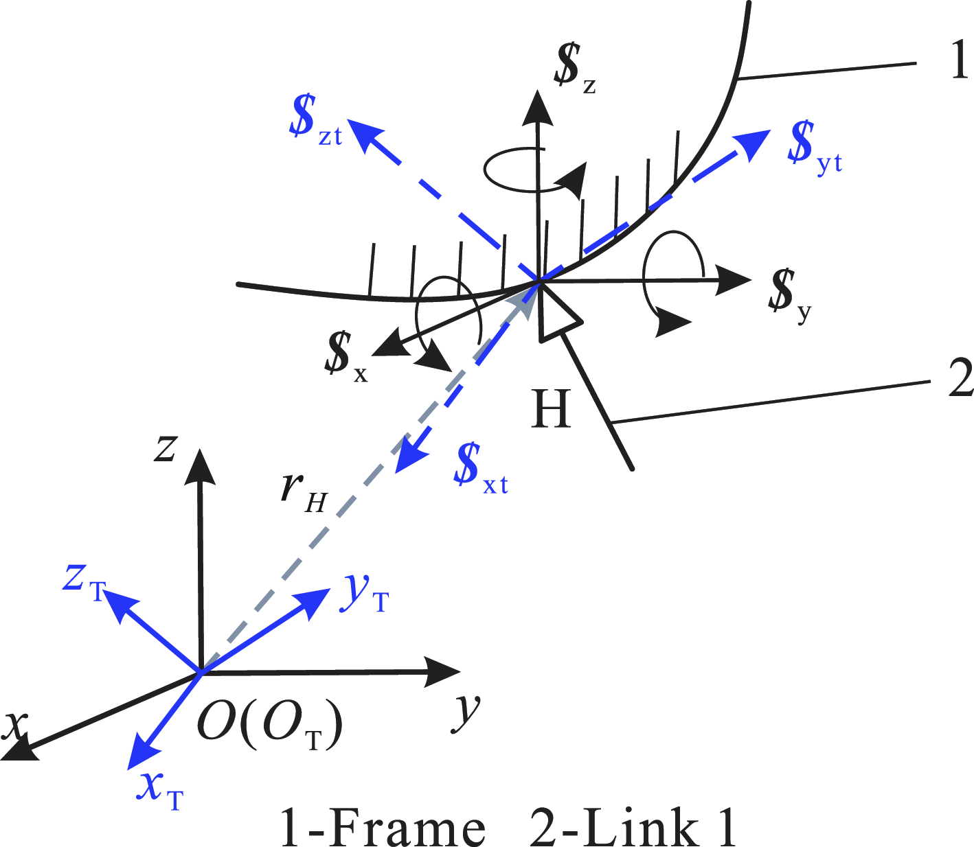
Therefore, the motion of a HKP is equivalent to three coupled prismatic pairs and three independent revolute pairs, see the Figure 3.
The screw of the higher kinematic pair.

By combining Eq. (8) and Eq. (9), the instantaneous screw of the HKP can be obtained,
 \begin{equation} \left\{\begin{array}{l} \textit{v}_{\mathrm{xt}}\boldsymbol{\$} _{\mathrm{xt}}=\textit{v}_{\mathrm{xt}}\left(\begin{array}{c} \boldsymbol{0}\\ \boldsymbol{s}_{\mathrm{xt}} \end{array}\right)\\[10pt] R_{\mathrm{a}}\textit{v}_{\mathrm{xt}}\boldsymbol{\$} _{\mathrm{yt}}=R_{\mathrm{a}}\textit{v}_{\mathrm{xt}}\left(\begin{array}{c} \boldsymbol{0}\\ \boldsymbol{s}_{\mathrm{yt}} \end{array}\right)\\[10pt] R_{\mathrm{b}}\textit{v}_{\mathrm{xt}}\boldsymbol{\$} _{\mathrm{zt}}=R_{\mathrm{b}}\textit{v}_{\mathrm{xt}}\left(\begin{array}{c} \boldsymbol{0}\\ \boldsymbol{s}_{\mathrm{zt}} \end{array}\right)\\[10pt] \omega _{\mathrm{x}}\boldsymbol{\$} _{\mathrm{x}}=\omega _{\mathrm{x}}\left(\begin{array}{c} \boldsymbol{s}_{\mathrm{x}}\\ \boldsymbol{r}_{\mathrm{H}}\times \boldsymbol{s}_{\mathrm{x}} \end{array}\right)\\ [10pt]\omega _{\mathrm{y}}\boldsymbol{\$} _{\mathrm{y}}=\omega _{y}\left(\begin{array}{c} \boldsymbol{s}_{y}\\ \boldsymbol{r}_{\mathrm{H}}\times \boldsymbol{s}_{y} \end{array}\right)\\[10pt] \omega _{\mathrm{z}}\boldsymbol{\$} _{\mathrm{z}}=\omega _{z}\left(\begin{array}{c} \boldsymbol{s}_{z}\\ \boldsymbol{r}_{\mathrm{H}}\times \boldsymbol{s}_{\mathrm{z}} \end{array}\right) \end{array}\right. \end{equation}
where there are four variables
 $\textit{v}_{\mathrm{xt}}, \omega _{\mathrm{x}}, \omega _{\mathrm{y}}$
, and
 $\omega _{\mathrm{z}}$
, it indicates that this kinematic pair has four DOFs.
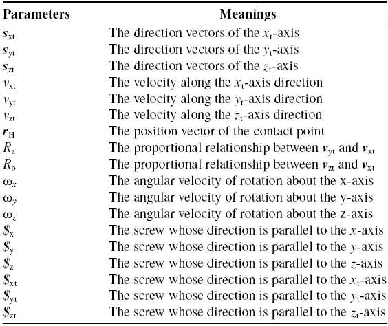
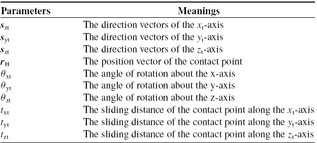
The meanings of all the parameters in the Eq. (10) are shown in the table 1.
The parameters in the instantaneous screw expression for higher kinematic pairs.

According to the approach for expressing the motion of a HKP by the instantaneous screw, the constraint matrix
 $\boldsymbol{M}_{\mathrm{h}}$
of the a single-loop HKP mechanism can be established. If there are i lower kinematic pairs and j HKP in a closed-loop mechanism, the kinematic equation can be listed according to Eq. (2),
 \begin{equation} \begin{array}{c} \omega _{1}\boldsymbol{\$} _{1}+\omega _{2}\boldsymbol{\$} _{2}+\ldots +\omega _{\mathrm{i}}\boldsymbol{\$} _{\mathrm{i}}+\boldsymbol{v}_{\mathrm{xt}1}\boldsymbol{\$} _{\mathrm{xt}1}+\boldsymbol{v}_{\mathrm{yt}1}\boldsymbol{\$} _{\mathrm{yt}1}+\boldsymbol{v}_{\mathrm{zt}1}\boldsymbol{\$} _{\mathrm{zt}1}\\ [10pt] +\boldsymbol{\$} _{\mathrm{s}1}\boldsymbol{\omega }_{\mathrm{s}1}+\ldots +\boldsymbol{v}_{\mathrm{xtj}}\boldsymbol{\$} _{\mathrm{xtj}}+\boldsymbol{v}_{\mathrm{ytj}}\boldsymbol{\$} _{\mathrm{ytj}}+\boldsymbol{v}_{\mathrm{ztj}}\boldsymbol{\$} _{\mathrm{ztj}}+\boldsymbol{\$} _{\mathrm{sj}}\boldsymbol{\omega }_{\mathrm{sj}}=\boldsymbol{0} \end{array} \end{equation}
therein,
 $\boldsymbol{\$} _{\mathrm{xtj}}, \boldsymbol{\$} _{\mathrm{ytj}}$
, and
 $\boldsymbol{\$} _{\mathrm{ztj}}$
are the screws along the three coordinate axes of the trajectory coordinate system of the j-th HKP.
 $\boldsymbol{v}_{\mathrm{xtj}}, \boldsymbol{v}_{\mathrm{ytj}}$
, and
 $\boldsymbol{v}_{\mathrm{ztj}}$
are the velocity components of sliding in the jth HKP.
 $\boldsymbol{\omega }_{\mathrm{sj}}$
and
 $\boldsymbol{\$} _{\mathrm{sj}}$
respectively represent the angular velocity and screw of the rotation in the jth HKP. In 3-dimensional space,
 $\boldsymbol{\omega }_{\mathrm{sj}}=(\begin{array}{l@{\quad}l@{\quad}l} \omega _{\mathrm{xj}} & \omega _{\mathrm{yj}} & \omega _{\mathrm{zj}} \end{array})^{\mathrm{T }}, \boldsymbol{\$} _{\mathrm{sj}}=(\begin{array}{l@{\quad}l@{\quad}l} \boldsymbol{\$} _{\mathrm{xj}} & \boldsymbol{\$} _{\mathrm{yj}} & \boldsymbol{\$} _{\mathrm{zj}} \end{array})$
.
According to the Eq. (7), the proportional relationship among
 $\boldsymbol{v}_{\mathrm{xtj}}, \boldsymbol{v}_{\mathrm{ytj}}$
, and
 $\boldsymbol{v}_{\mathrm{ztj}}$
is as follows,
 \begin{equation} \begin{array}{c} R_{\mathrm{aj}}\boldsymbol{v}_{\mathrm{xtj}}-\boldsymbol{v}_{\mathrm{ytj}}=0\\[5pt] R_{\mathrm{bj}}\boldsymbol{v}_{\mathrm{xtj}}-\boldsymbol{v}_{\mathrm{ztj}}=0 \end{array} \end{equation}
where
 $R_{\mathrm{aj}}$
are the proportional relationship between
 $\boldsymbol{v}_{\mathrm{ytj}}$
and
 $\boldsymbol{v}_{\mathrm{xtj}}, R_{\mathrm{bj}}$
are the proportional relationship between
 $\boldsymbol{v}_{\mathrm{ztj}}$
and
 $\boldsymbol{v}_{\mathrm{xtj}}$
.
Combining Eq. (11) and Eq. (12),
 \begin{equation} \left\{\begin{array}{l} \omega _{1}\boldsymbol{\$} _{1}+\omega _{2}\boldsymbol{\$} _{2}+\ldots +\omega _{\mathrm{i}}\boldsymbol{\$} _{\mathrm{i}}+\boldsymbol{v}_{\mathrm{xt}1}\boldsymbol{\$} _{\mathrm{xt}1}+\boldsymbol{v}_{\mathrm{yt}1}\boldsymbol{\$} _{\mathrm{yt}1}+\\ \boldsymbol{v}_{\mathrm{zt}1}\boldsymbol{\$} _{\mathrm{zt}1}+\boldsymbol{\$} _{\mathrm{s}1}\boldsymbol{\omega }_{\mathrm{s}1}+\ldots +\boldsymbol{v}_{\mathrm{xtj}}\boldsymbol{\$} _{\mathrm{xtj}}+\boldsymbol{v}_{\mathrm{ytj}}\boldsymbol{\$} _{\mathrm{ytj}}+\boldsymbol{v}_{\mathrm{ztj}}\boldsymbol{\$} _{\mathrm{ztj}}+\boldsymbol{\$} _{\mathrm{sj}}\boldsymbol{\omega }_{\mathrm{sj}}=\boldsymbol{0} \\ \qquad \qquad \qquad R_{\mathrm{a}1}\boldsymbol{v}_{\mathrm{xt}1}-\boldsymbol{v}_{\mathrm{yt}1}=0\\ \qquad \qquad \qquad R_{\mathrm{b}1}\boldsymbol{v}_{\mathrm{xt}1}-\boldsymbol{v}_{\mathrm{zt}1}=0\\ \quad \qquad \qquad \qquad \qquad \vdots \\ \qquad \qquad \qquad R_{\mathrm{aj}}\boldsymbol{v}_{\mathrm{xtj}}-\boldsymbol{v}_{\mathrm{ytj}}=0\\ \qquad \qquad \qquad R_{\mathrm{bj}}\boldsymbol{v}_{\mathrm{xtj}}-\boldsymbol{v}_{\mathrm{ztj}}=0 \end{array}\right. \end{equation}
Equation (13) can be expressed as,
 \begin{equation} \left(\begin{array}{c@{\quad}c@{\quad}c@{\quad}c@{\quad}c@{\quad}c@{\quad}c@{\quad}c@{\quad}c@{\quad}c@{\quad}c@{\quad}c@{\quad}c} \boldsymbol{\$} _{1} & \boldsymbol{\$} _{2} & \cdots & \boldsymbol{\$} _{\mathrm{i}} & \boldsymbol{\$} _{\mathrm{xt}1} & \boldsymbol{\$} _{\mathrm{yt}1} & \boldsymbol{\$} _{\mathrm{zt}1} & \boldsymbol{\$} _{\mathrm{S}1} & \cdots & \boldsymbol{\$} _{\mathrm{xtj}} & \boldsymbol{\$} _{\mathrm{ytj}} & \boldsymbol{\$} _{\mathrm{ztj}} & \boldsymbol{\$} _{\mathrm{Sj}}\\ 0 & 0 & \ldots & 0 & R_{\mathrm{a}1} & -1 & 0 & 0 & \cdots & 0 & 0 & 0 & 0\\ 0 & 0 & \cdots & 0 & R_{\mathrm{b}1} & 0 & -1 & 0 & \cdots & 0 & 0 & 0 & 0\\ \vdots & \vdots & \vdots & \vdots & \vdots & \vdots & \vdots & \vdots & \vdots & \vdots & \vdots & \vdots & \vdots \\ 0 & 0 & \cdots & 0 & 0 & 0 & 0 & 0 & \cdots & R_{\mathrm{aj}} & -1 & 0 & 0\\ 0 & 0 & \cdots & 0 & 0 & 0 & 0 & 0 & \cdots & R_{\mathrm{bj}} & 0 & -1 & 0 \end{array}\right)\left(\begin{array}{c} \omega _{1}\\ \omega _{2}\\ \vdots \\ \omega _{\mathrm{i}}\\ \boldsymbol{v}_{\mathrm{xt}1}\\ \boldsymbol{v}_{\mathrm{yt}1}\\ \boldsymbol{v}_{\mathrm{zt}1}\\ \boldsymbol{\omega }_{\mathrm{s}1}\\ \vdots \\ \boldsymbol{v}_{\mathrm{xtj}}\\ \boldsymbol{v}_{\mathrm{ytj}}\\ \boldsymbol{v}_{\mathrm{ztj}}\\ \boldsymbol{\omega }_{\mathrm{sj}} \end{array}\right)=0 \end{equation}
Therefore, the constraint matrix of this HKP mechanism can be written as,
 \begin{equation} \boldsymbol{M}_{\mathrm{h}}=\left(\begin{array}{c@{\quad}c@{\quad}c@{\quad}c@{\quad}c@{\quad}c@{\quad}c@{\quad}c@{\quad}c@{\quad}c@{\quad}c@{\quad}c@{\quad}c} \boldsymbol{\$} _{1} & \boldsymbol{\$} _{2} & \cdots & \boldsymbol{\$} _{\mathrm{i}} & \boldsymbol{\$} _{\mathrm{xt1}} & \boldsymbol{\$} _{\mathrm{yt}1} & \boldsymbol{\$} _{\mathrm{zt}1} & \boldsymbol{\$} _{\mathrm{S}1} & \cdots & \boldsymbol{\$} _{\mathrm{xtj}} & \boldsymbol{\$} _{\mathrm{ytj}} & \boldsymbol{\$} _{\mathrm{ztj}} & \boldsymbol{\$} _{\mathrm{Sj}}\\ 0 & 0 & \ldots & 0 & R_{\mathrm{a}1} & -1 & 0 & 0 & \cdots & 0 & 0 & 0 & 0\\ 0 & 0 & \cdots & 0 & R_{\mathrm{b}1} & 0 & -1 & 0 & \cdots & 0 & 0 & 0 & 0\\ \vdots & \vdots & \vdots & \vdots & \vdots & \vdots & \vdots & \vdots & \vdots & \vdots & \vdots & \vdots & \vdots \\ 0 & 0 & \cdots & 0 & 0 & 0 & 0 & 0 & \cdots & R_{\mathrm{aj}} & -1 & 0 & 0\\ 0 & 0 & \cdots & 0 & 0 & 0 & 0 & 0 & \cdots & R_{\mathrm{bj}} & 0 & -1 & 0 \end{array}\right) \end{equation}
At this time, the DOF of the HKP mechanism can be obtained as,
 \begin{equation} m_{\mathrm{h}}=\text{nullity}(\boldsymbol{M}_{\mathrm{h}})=n_{\mathrm{h}}-\text{rank}(\boldsymbol{M}_{\mathrm{h}}) \end{equation}
It should be noticed that the result may contains local degree-of-freedom, namely, the local rotation formed between two spherical pairs, the rotational DOF of the roller in a cam mechanism, and the axes of multiple revolute pairs or the trajectories of sliding pair in a mechanism are parallel to each other. For the output motion of a mechanism, a local DOF is often a redundant DOF and it has no influence on the output DOF of the mechanism. Therefore, the final DOF neglecting the local ones is
 \begin{equation} m_{\mathrm{h}}^{'}=m_{\mathrm{h}}-\zeta \end{equation}
where
 $\zeta$
is the number of local DOF.
3. The finite screw theory for the mechanisms with higher kinematic pairs
The finite screw theory can be used to describe the motion displacement of a mechanism. Through the finite screw theory, we can obtain the pose of the end rigid body relative to the reference configuration. And it has only six algebraic elements, which can clearly and intuitively reflect the three elements of Chasles. It is the “simplest” description format of the finite motion of a rigid body [Reference Yang, Sun, Huang, Li and Gu33]. According to Chasles’ finite displacement theorem, the representation of the finite displacement
 $\boldsymbol{S}_{\mathrm{f}}$
of a rigid body in the Plücker coordinate format as follows:
 \begin{equation} \boldsymbol{S}_{\mathrm{f}}=2\tan \frac{\theta _{\mathrm{f}}}{2}\left(\begin{array}{c} \boldsymbol{s}_{{\mathrm{f}}}\\ \boldsymbol{r}_{\mathrm{f}}\times \boldsymbol{s}_{{\mathrm{f}}} \end{array}\right)+t_{\mathrm{f}}\left(\begin{array}{c} \boldsymbol{0}\\ \boldsymbol{s}_{{\mathrm{f}}} \end{array}\right) \end{equation}
Therein,
 $\theta _{\mathrm{f}}$
is the rotation angle of the rigid body around the axis relative to the initial position,
 $t_{\mathrm{f}}$
is the moving distance of the rigid body along the axis relative to the initial position,
 $\boldsymbol{s}_{\mathrm{f}}$
is the direction vector of the axis,
 $\boldsymbol{r}_{\mathrm{f}}$
is the position vector of a point on the axis.
In the finite screw theory, the motion synthesis of serial kinematic pairs can be calculated by using the screw triangle product [Reference Sun, Yang, Huang and Dai34]. In this way, the analytical expressions of the mechanism and its finite motion of kinematic chain can be directly established.
 \begin{equation} \boldsymbol{S}_{12}=\boldsymbol{S}_{1}{\unicode[Arial]{x0394}} \boldsymbol{S}_{2}=\frac{\boldsymbol{S}_{1}+\boldsymbol{S}_{2}+\dfrac{\boldsymbol{S}_{1}\times \boldsymbol{S}_{2}}{2}-\tan \dfrac{\theta _{1}}{2}\tan \dfrac{\theta _{2}}{2}\left(t_{1}\left(\begin{array}{c} \boldsymbol{0}\\ \boldsymbol{s}_{1} \end{array}\right)+t_{1}\left(\begin{array}{c} \boldsymbol{0}\\ \boldsymbol{s}_{2} \end{array}\right)\right)}{1-\tan \dfrac{\theta _{1}}{2}\tan \dfrac{\theta _{2}}{2}\boldsymbol{s}_{1}^{\mathrm{T }}\boldsymbol{s}_{\boldsymbol{2}}} \end{equation}
Therein,
 $\boldsymbol{S}_{\mathrm{i}}=2\tan \dfrac{\theta _{\mathrm{i}}}{2}\left(\begin{array}{c} \boldsymbol{s}_{{\mathrm{i}}}\\ \boldsymbol{r}_{\mathrm{i}}\times \boldsymbol{s}_{\mathrm{i}} \end{array}\right)+t_{\mathrm{i}}\left(\begin{array}{c} \boldsymbol{0}\\ \boldsymbol{s}_{\mathrm{i}} \end{array}\right),i=1,2, {\unicode[Arial]{x0394}}$
is the screw triangle synthesis operation.
Based on the above analysis of the decomposition of the motion of the HKP, the motion of a higher kinematic pair is equivalent to three coupled prismatic pairs and three independent revolute pairs, so its finite motion is shown in Figure 4.
The finite motion of the higher kinematic pair.

Since the HKP is in point contact and the contact point always moves along the trajectory of the HKP, the three coupled prismatic pairs can be regarded as three consecutive translations of the contact point. Therefore, the three prismatic pairs are in a series relationship. According to the motion synthesis principle of the finite screw, the finite screw for sliding along the trajectory can be written as,
 \begin{equation} \boldsymbol{S}_{\mathrm{h}1}=t_{\mathrm{xt}}\left(\begin{array}{c} \boldsymbol{0}\\ \boldsymbol{s}_{\mathrm{xt}} \end{array}\right){\unicode[Arial]{x0394}} t_{\mathrm{yt}}\left(\begin{array}{c} \boldsymbol{0}\\ \boldsymbol{s}_{\mathrm{yt}} \end{array}\right){\unicode[Arial]{x0394}} t_{\mathrm{zt}}\left(\begin{array}{c} \boldsymbol{0}\\ \boldsymbol{s}_{\mathrm{zt}} \end{array}\right) \end{equation}
where
 $\boldsymbol{S}_{\mathrm{h}1}$
is the finite screw of sliding along the trajectory of HKP.
 $t_{\mathrm{xt}}, t_{\mathrm{yt}}$
, and
 $t_{\mathrm{zt}}$
are the components in three directions of the
 $O_{\mathrm{T}}-x_{\mathrm{T}}y_{\mathrm{T}}z_{\mathrm{T}}$
for the distance that point H moves along the trajectory C, respectively.
 $\boldsymbol{s}_{\mathrm{xt}}, \boldsymbol{s}_{\mathrm{yt}}$
, and
 $\boldsymbol{s}_{\mathrm{zt}}$
respectively represent the direction vectors of the three coordinate axes of the
 $O_{\mathrm{T}}-x_{\mathrm{T}}y_{\mathrm{T}}z_{\mathrm{T}}$
.
Due to the point H always moves along the trajectory C, the relationship between
 $t_{\mathrm{xt}}, t_{\mathrm{yt}}$
, and
 $t_{\mathrm{zt}}$
satisfies its trajectory equation, i.e.,
 \begin{equation} \left\{\begin{array}{c} t_{\mathrm{xt}}=x\left(t\right)-x\left(0\right)\\ t_{\mathrm{yt}}=y\left(t\right)-y\left(0\right)\\ t_{\mathrm{zt}}=z\left(t\right)-z\left(0\right) \end{array}\right. \end{equation}
Therein,
 $\left\{\begin{array}{c} x\left(t\right)\\ y\left(t\right)\\ z\left(t\right) \end{array}\right.$
represents the parametric equation of the trajectory C,
 $\left\{\begin{array}{c} x\left(0\right)\\ y\left(0\right)\\ z\left(0\right) \end{array}\right.$
represents the initial position of the HKP.
The finite screw for rotating around contact point H can be written as
 \begin{equation} \boldsymbol{S}_{\mathrm{h}2}=2\tan \frac{\theta _{\mathrm{z}}}{2}\left(\begin{array}{c} \boldsymbol{s}_{\mathrm{zt}}\\ \boldsymbol{r}_{\mathrm{H}}\times \boldsymbol{s}_{\mathrm{zt}} \end{array}\right){\unicode[Arial]{x0394}} 2\tan \frac{\theta _{\mathrm{y}}}{2}\left(\begin{array}{c} \boldsymbol{s}_{\mathrm{yt}}\\ \boldsymbol{r}_{\mathrm{H}}\times \boldsymbol{s}_{\mathrm{yt}} \end{array}\right){\unicode[Arial]{x0394}} 2\tan \frac{\theta _{\mathrm{x}}}{2}\left(\begin{array}{c} \boldsymbol{s}_{\mathrm{xt}}\\ \boldsymbol{r}_{\mathrm{H}}\times \boldsymbol{s}_{\mathrm{xt}} \end{array}\right) \end{equation}
Therein,
 $\boldsymbol{S}_{\mathrm{h}2}$
is the finite screw of rotation around contact point H.
 $\theta _{\mathrm{z}}, \theta _{\mathrm{y}}$
, and
 $\theta _{\mathrm{x}}$
, respectively, are the rotation angles around the three coordinate axes of the coordinate system
 $O_{\mathrm{T}}-x_{\mathrm{T}}y_{\mathrm{T}}z_{\mathrm{T}}$
.
 $\boldsymbol{r}_{\mathrm{H}}$
is the position vector of the contact point H in the global coordinate system
 $O-xyz$
.
And the sliding along the trajectory and the rotation around contact point of HKP and are in series. Therefore, according to the synthesis criterion of the finite screw theory, the finite screw of the entire HKP can be expressed as
 \begin{align} \boldsymbol{S}_{\mathrm{h}} & =\boldsymbol{S}_{\mathrm{h}2}{\unicode[Arial]{x0394}} \boldsymbol{S}_{\mathrm{h}1} \nonumber \\ & =2\tan \dfrac{\theta _{\mathrm{zt}}}{2}\left(\begin{array}{c} \boldsymbol{s}_{\mathrm{zt}}\\ \boldsymbol{r}_{\mathrm{H}}\times \boldsymbol{s}_{\mathrm{zt}} \end{array}\right){\unicode[Arial]{x0394}} 2\tan \dfrac{\theta _{\mathrm{yt}}}{2}\left(\begin{array}{c} \boldsymbol{s}_{\mathrm{yt}}\\ \boldsymbol{r}_{\mathrm{H}}\times \boldsymbol{s}_{\mathrm{yt}} \end{array}\right){\unicode[Arial]{x0394}} 2\tan \dfrac{\theta _{\mathrm{xt}}}{2}\left(\begin{array}{c} \boldsymbol{s}_{\mathrm{xt}}\\ \boldsymbol{r}_{\mathrm{H}}\times \boldsymbol{s}_{\mathrm{xt}} \end{array}\right) \nonumber \\ & \quad {\unicode[Arial]{x0394}} t_{\mathrm{xt}}\left(\begin{array}{c} \boldsymbol{0}\\ \boldsymbol{s}_{\mathrm{xt}} \end{array}\right){\unicode[Arial]{x0394}} t_{\mathrm{yt}}\left(\begin{array}{c} \boldsymbol{0}\\ \boldsymbol{s}_{\mathrm{yt}} \end{array}\right){\unicode[Arial]{x0394}} t_{\mathrm{zt}}\left(\begin{array}{c} \boldsymbol{0}\\ \boldsymbol{s}_{\mathrm{zt}} \end{array}\right) \end{align}
The meanings of all the parameters in the Eq. (23) are shown in the Table II.
The parameters in the finite screw expression for higher kinematic pairs.

4. Kinematic analysis examples by the proposed approach
4.1. Planar cam-linkage mechanism
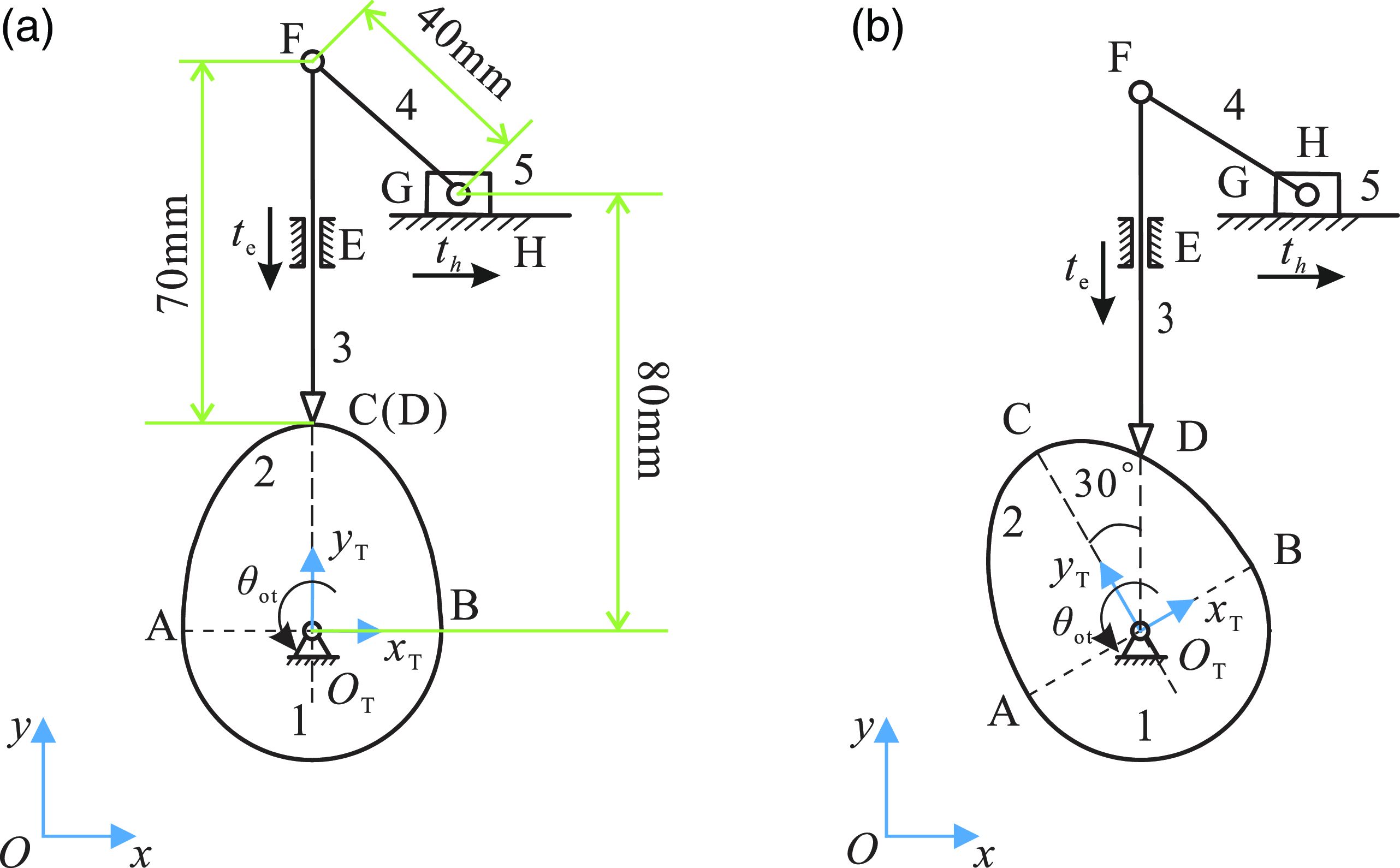
For a planar cam-linkage mechanism in Figure 5, its initial position is shown as Figure 5(a). Figure 5(a) is the initial position, with the displacements of both revolute joints and prismatic joints are being zero. Figure 5(b) is the position of the cam after being turned through 30°. The coordinate system
 $O-xy$
is a global coordinate system, and the coordinate system
 $O_{\mathrm{T}}-x_{\mathrm{T}}y_{\mathrm{T}}$
is the trajectory coordinate system of the HKP,
 $l_{\mathrm{DF}}=70\mathrm{mm},l_{\mathrm{FG}}=40\mathrm{mm}$
, the parametric equation of the arc ACB under the coordinate system
 $O_{\mathrm{T}}-x_{\mathrm{T}}y_{\mathrm{T}}$
is
 $\left\{\begin{array}{c} x=25\sin t\\ y=40\cos t \end{array}\right.,t\in \left(-\dfrac{\pi }{2},\dfrac{\pi }{2}\right)$
. The arc AB is a section of the arc with an radius of 25 mm, and the vertical distance from point G to
 $O_{\mathrm{T}}$
is 80 mm.
Planar cam-linkage mechanism.

(1) DOF analysis of the mechanism by the G-K formula
In a plane, the G-K formula for calculating the DOF is
 \begin{equation} \mathrm{m}_{\mathrm{G}}=3n-2P_{\mathrm{L}}-P_{\mathrm{H}} \end{equation}
where m G represents the DOF of the mechanism, n is the number of moving components in the mechanism, P L is the number of lower pairs, P H is the number of higher pairs.
Therefore, the DOF of this mechanism obtained,
 \begin{equation} \mathrm{m}_{\mathrm{G}}=3n-2P_{\mathrm{L}}-P_{\mathrm{H}}=3\times 4-2\times 5-1=1 \end{equation}
(2) DOF analysis of the mechanism by the instantaneous screw theory
When the cam is in the position of Figure 5(b), we can obtain the
 $\dfrac{x}{y}=\dfrac{25\sin t}{40\cos t}=\tan 30^{\circ}$
in the
 $O_{\mathrm{T}}-x_{\mathrm{T}}y_{\mathrm{T}}$
, so the parameters of the corresponding trajectory equations is
 $\mathrm{t}=\arctan \dfrac{8\sqrt{3}}{15}$
.
The positions of each point in the figure are
 \begin{equation} \begin{array}{l} \boldsymbol{O}_{\mathrm{T}}=\left(\begin{array}{l@{\quad}l@{\quad}l} 40 & 40 & 0 \end{array}\right)^{\mathrm{T }}\mathrm{,}\ \boldsymbol{D}=\left(\begin{array}{l@{\quad}l@{\quad}l} 40 & 40+\sqrt{x^{2}+y^{2}} & 0 \end{array}\right)^{\mathrm{T }},\\[10pt] \boldsymbol{F}=\left(\begin{array}{l@{\quad}l@{\quad}l} 40 & 110+\sqrt{x^{2}+y^{2}} & 0 \end{array}\right)^{\mathrm{T }}\mathrm{,}\ \boldsymbol{G}=\left(\begin{array}{l@{\quad}l@{\quad}l} 40+\sqrt{40^{2}-\left(70+\sqrt{x^{2}+y^{2}}\right)^{2}} & 120 & 0 \end{array}\right)^{\mathrm{T }} \end{array} \end{equation}
Since it is a planar mechanism, the direction vectors of all revolute pairs are
 $\boldsymbol{s}_{\mathrm{z}}=(\begin{array}{l@{\quad}l@{\quad}l} 0 & 0 & 1 \end{array})^{\mathrm{T }}$
, the direction vectors of the prismatic pair E and the prismatic pair H are
 $\boldsymbol{s}_{\mathrm{e}}=(\begin{array}{l@{\quad}l@{\quad}l} 0 & 1 & 0 \end{array})^{\mathrm{T }}$
and
 $\boldsymbol{s}_{\mathrm{h}}=(\begin{array}{l@{\quad}l@{\quad}l} 1 & 0 & 0 \end{array})^{\mathrm{T }}$
, respectively. The direction vectors of the
 $x_{\mathrm{T}}$
-axis and
 $y_{\mathrm{T}}$
-axis of the trajectory coordinate system are
 $\boldsymbol{s}_{\mathrm{xt}}=\left(\begin{array}{l@{\quad}l@{\quad}l} \dfrac{\sqrt{3}}{2} & \dfrac{1}{2} & 0 \end{array}\right)^{\mathrm{T }}$
and
 $\boldsymbol{s}_{\mathrm{yt}}=\left(\begin{array}{l@{\quad}l@{\quad}l} -\dfrac{1}{2} & \dfrac{\sqrt{3}}{2} & 0 \end{array}\right)^{\mathrm{T }}$
.
Therefore, the screws of each kinematic pair can be written as
 \begin{equation} \begin{array}{l} \boldsymbol{\$} _{\mathrm{OT}}=\left(\begin{array}{c} \boldsymbol{s}_{\mathrm{z}}\\ \boldsymbol{O}_{\mathrm{T }}\times \boldsymbol{s}_{\mathrm{z}} \end{array}\right)\mathrm{,}\ \boldsymbol{\$} _{\mathrm{E}}=\left(\begin{array}{c} \mathbf{0}\\ \boldsymbol{s}_{\mathrm{e}} \end{array}\right)\mathrm{,}\ \boldsymbol{\$} _{\mathrm{F}}=\left(\begin{array}{c} \boldsymbol{s}_{\mathrm{z}}\\ \boldsymbol{F}\times \boldsymbol{s}_{\mathrm{z}} \end{array}\right)\mathrm{,}\ \boldsymbol{\$} _{\mathrm{G}}=\left(\begin{array}{c} \boldsymbol{s}_{\mathrm{z}}\\ \boldsymbol{G}\times \boldsymbol{s}_{\mathrm{z}} \end{array}\right)\\[10pt] \boldsymbol{\$} _{\mathrm{H}}=\left(\begin{array}{c} \mathbf{0}\\ \boldsymbol{s}_{\mathrm{h}} \end{array}\right)\mathrm{,}\ \boldsymbol{\$} _{\mathrm{D}}=\left(\begin{array}{c} \boldsymbol{s}_{\mathrm{z}}\\ \boldsymbol{D}\times \boldsymbol{s}_{\mathrm{z}} \end{array}\right)\mathrm{,}\ \boldsymbol{\$} _{\mathrm{xt}}=\left(\begin{array}{c} \mathbf{0}\\ \boldsymbol{s}_{\mathrm{xt}} \end{array}\right)\mathrm{,}\ \boldsymbol{\$} _{\mathrm{yt}}=\left(\begin{array}{c} \mathbf{0}\\ \boldsymbol{s}_{\mathrm{yt}} \end{array}\right) \end{array} \end{equation}
The velocity ratio of movement along the
 $x_{\mathrm{T}}$
-axis and
 $y_{\mathrm{T}}$
-axis are obtained,
 \begin{equation} R=\frac{\boldsymbol{v}_{\mathrm{yt}}}{\boldsymbol{v}_{\mathrm{xt}}}=\frac{dy}{dx}=\frac{dy/dt}{dx/dt}=\frac{25\cos \left(\arctan \dfrac{8\sqrt{3}}{15}\right)}{-40\sin \left(\arctan \dfrac{8\sqrt{3}}{15}\right)}\approx -1.4780 \end{equation}
Therefore, its constraint matrix be obtained as
 \begin{equation} \boldsymbol{M}_{{\mathrm{{h}_{{13\times 8}}}}}=\left(\begin{array}{l@{\quad}l@{\quad}l@{\quad}l@{\quad}l@{\quad}l@{\quad}l@{\quad}l} \boldsymbol{\$} _{\mathrm{OT}} & \boldsymbol{\$} _{\mathrm{D}} & \boldsymbol{\$} _{xt} & \boldsymbol{\$} _{yt} & \boldsymbol{\$} _{\mathrm{E}} & Q & Q & Q\\ Q & Q & Q & Q & -\boldsymbol{\$} _{\mathrm{E}} & \boldsymbol{\$} _{\mathrm{F}} & \boldsymbol{\$} _{\mathrm{G}} & \boldsymbol{\$} _{\mathrm{H}}\\ 0 & 0 & R & -1 & 0 & 0 & 0 & 0 \end{array}\right) \end{equation}
where
 $\boldsymbol{Q}\boldsymbol{=}(\begin{array}{l@{\quad}l@{\quad}l@{\quad}l@{\quad}l@{\quad}l} 0 & 0 & 0 & 0 & 0 & 0 \end{array})^{\mathrm{T }}$
.
The rank of the constraint matrix is obtained by using MATLAB,
 $\mathrm{rank}(\boldsymbol{M}_{{\mathrm{{h}_{{13\times 8}}}}})=7$
. Since the dimension of the constraint matrix is
 $13\times 8$
, the degree of freedom of this mechanism obtained,
 \begin{equation} m_{\mathrm{h}}=n_{\mathrm{h}}-\text{rank} \! \left(\boldsymbol{M}_{{\mathrm{{h}_{{13\times 8}}}}}\right)=8-7=1 \end{equation}
The result has been validated through the technique of CAD in Solidworks, see the supplementary video, and both approaches for calculating DOF are correct
(3) Analysis of kinematic relationship between the motion angles by the finite screw theory
As shown in Figure 5(a), at this time, the trajectory coordinate system of HKP is parallel to the global coordinate system. The moving distance of the contact point of the higher pair is
 $\left\{\begin{array}{c} t_{\mathrm{xt}}=x\left(t\right)-x\left(0\right)\\ t_{\mathrm{yt}}=y\left(t\right)-y\left(0\right) \end{array}\right.$
, the positions of each point in the figure are
 \begin{equation} \boldsymbol{O}_{\mathrm{T}}=\left(\begin{array}{l@{\quad}l@{\quad}l} 40 & 40 & 0 \end{array}\right)^{\mathrm{T }}\mathrm{,}\ \boldsymbol{D}=\left(\begin{array}{l@{\quad}l@{\quad}l} 40 & 80 & 0 \end{array}\right)^{\mathrm{T }}\mathrm{,}\ \boldsymbol{F}=\left(\begin{array}{l@{\quad}l@{\quad}l} 40 & 150 & 0 \end{array}\right)^{\mathrm{T }}\mathrm{,}\ \boldsymbol{G}=\left(\begin{array}{l@{\quad}l@{\quad}l} 40+10\sqrt{7} & 120 & 0 \end{array}\right)^{\mathrm{T }} . \end{equation}
At this time, the direction vectors of the axes of the trajectory coordinate system are
 $\boldsymbol{s}_{\mathrm{xt}}=(\begin{array}{l@{\quad}l@{\quad}l} 1 & 0 & 0 \end{array})^{\mathrm{T }}, \boldsymbol{s}_{\mathrm{yt}}=(\begin{array}{l@{\quad}l@{\quad}l} 0 & 1 & 0 \end{array})^{\mathrm{T }}$
, respectively.
Therefore, the finite screws of each kinematic pair can be written as
 \begin{equation} \begin{array}{c} \boldsymbol{S}_{\mathrm{OT}}=2\tan \dfrac{\theta _{\mathrm{ot}}}{2}\left(\begin{array}{c} \boldsymbol{s}_{\mathrm{z}}\\ \boldsymbol{O}_{\mathrm{T }}\times \boldsymbol{s}_{\mathrm{z}} \end{array}\right)\mathrm{,}\ \boldsymbol{S}_{\mathrm{G}}=2\tan \dfrac{\theta _{\mathrm{g}}}{2}\left(\begin{array}{c} \boldsymbol{s}_{\mathrm{z}}\\ \boldsymbol{G}\times \boldsymbol{s}_{\mathrm{z}} \end{array}\right)\mathrm{,}\ \boldsymbol{S}_{\mathrm{F}}=2\tan \dfrac{\theta _{\mathrm{f}}}{2}\left(\begin{array}{c} \boldsymbol{s}_{\mathrm{z}}\\ \boldsymbol{F}\times \boldsymbol{s}_{\mathrm{z}} \end{array}\right)\\[10pt] \boldsymbol{S}_{\mathrm{E}}=t_{\mathrm{e}}\left(\begin{array}{c} \mathbf{0}\\ \boldsymbol{s}_{\mathrm{e}} \end{array}\right)\mathrm{,}\ \boldsymbol{S}_{\mathrm{H}}=t_{\mathrm{h}}\left(\begin{array}{c} \mathbf{0}\\ \boldsymbol{s}_{\mathrm{h}} \end{array}\right)\mathrm{,}\ \boldsymbol{S}_{\mathrm{h}}=t_{\mathrm{xt}}\left(\begin{array}{c} \mathbf{0}\\ \boldsymbol{s}_{\mathrm{xt}} \end{array}\right){\unicode[Arial]{x0394}} t_{\mathrm{yt}}\left(\begin{array}{c} \mathbf{0}\\ \boldsymbol{s}_{\mathrm{yt}} \end{array}\right){\unicode[Arial]{x0394}} 2\tan \dfrac{\theta _{\mathrm{d}}}{2}\left(\begin{array}{c} \boldsymbol{s}_{\mathrm{z}}\\ \boldsymbol{D}\times \boldsymbol{s}_{\mathrm{z}} \end{array}\right) \end{array} \end{equation}
The finite screw of the first kinematic loop can be written as
 \begin{equation} \boldsymbol{S}_{1}=-\boldsymbol{S}_{\mathrm{E}}{\unicode[Arial]{x0394}} \boldsymbol{S}_{\mathrm{h}}{\unicode[Arial]{x0394}} \boldsymbol{S}_{\mathrm{OT}}=\mathbf{0} \end{equation}
The finite screw of the second kinematic loop can be written as
 \begin{equation} \boldsymbol{S}_{2}=-\boldsymbol{S}_{\mathrm{H}}{\unicode[Arial]{x0394}} \boldsymbol{S}_{\mathrm{G}}{\unicode[Arial]{x0394}} \boldsymbol{S}_{\mathrm{F}}{\unicode[Arial]{x0394}} \boldsymbol{S}_{\mathrm{E}}=\mathbf{0} \end{equation}
The relationships between the cam rotation angle
 $\theta _{\mathrm{ot}}$
and the displacements
 $t_{\mathrm{e}}$
of the prismatic pair E as well as the displacements
 $t_{\mathrm{h}}$
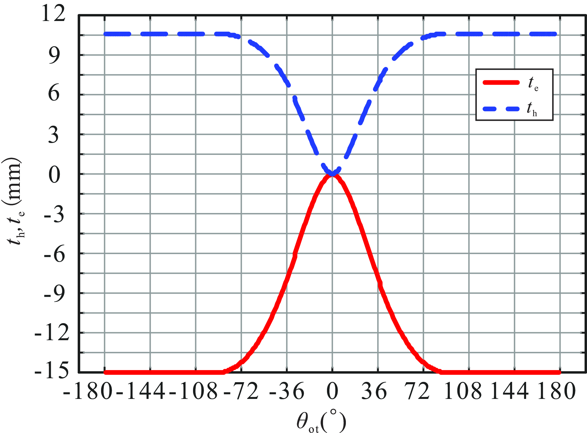
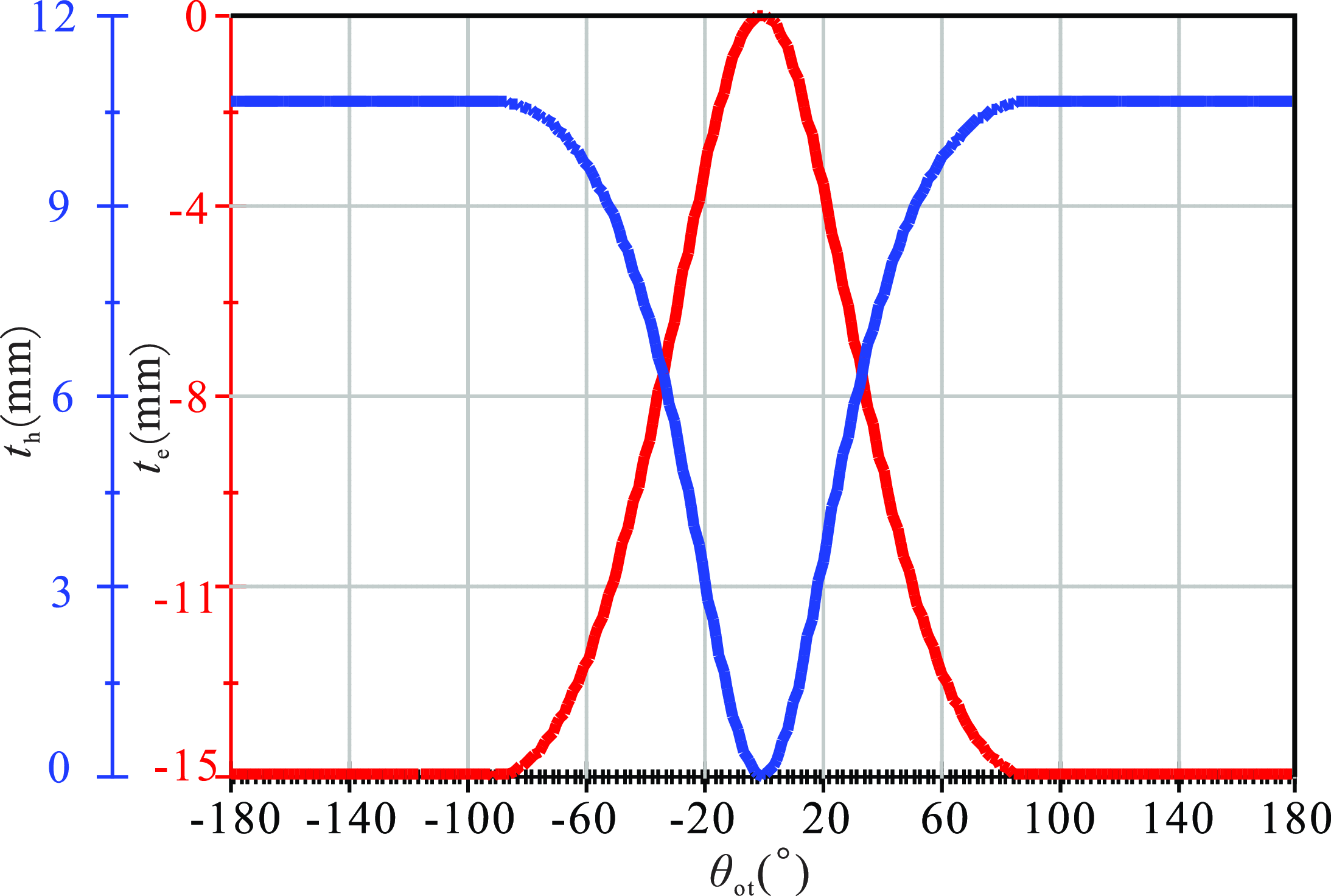
of the prismatic pair H can be solved, respectively, by combining Eq.(33) and Eq. (34). The result is shown in Figure 6.
The relationship between cam rotation angle and displacement of prismatic pair.

As can be seen from the Figure 6, the rotation of the cam can drive the vertical reciprocating motion of slider E, thereby driving the horizontal reciprocating motion of slider H.
The motion module of Solidwroks provides an effective tool for kinematic analysis. Therefore, this module is employed to validate the results by conducting simulations for the planar cam-linkage mechanism, and the resulting graphical analysis is presented in Figure 7.
The simulation results of planar cam-linkage mechanism.

By comparing Figure 6 and Figure 7, it can be observed that the simulation results are in complete agreement with the results calculated using this method.
4.2. Cylindrical cam mechanism
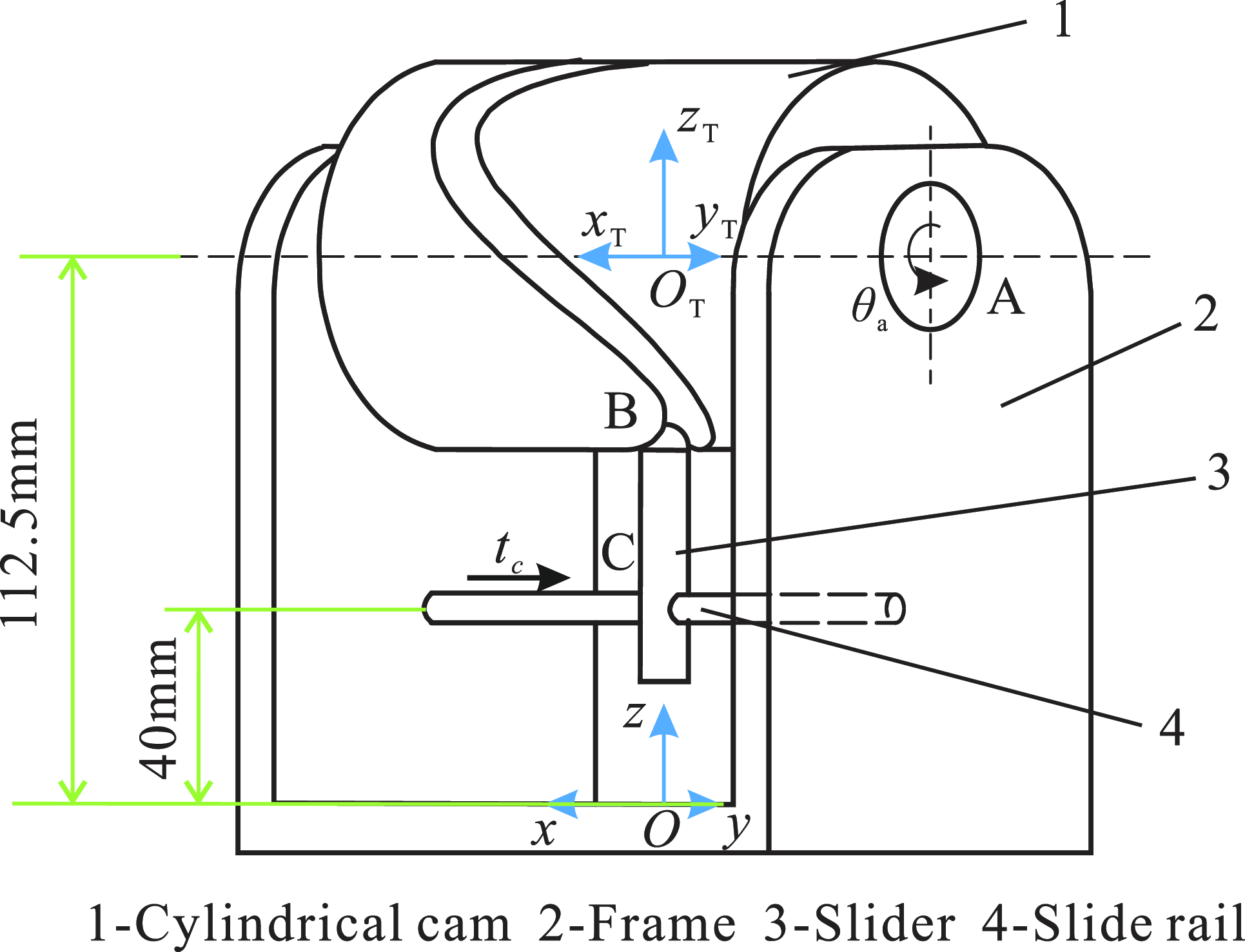
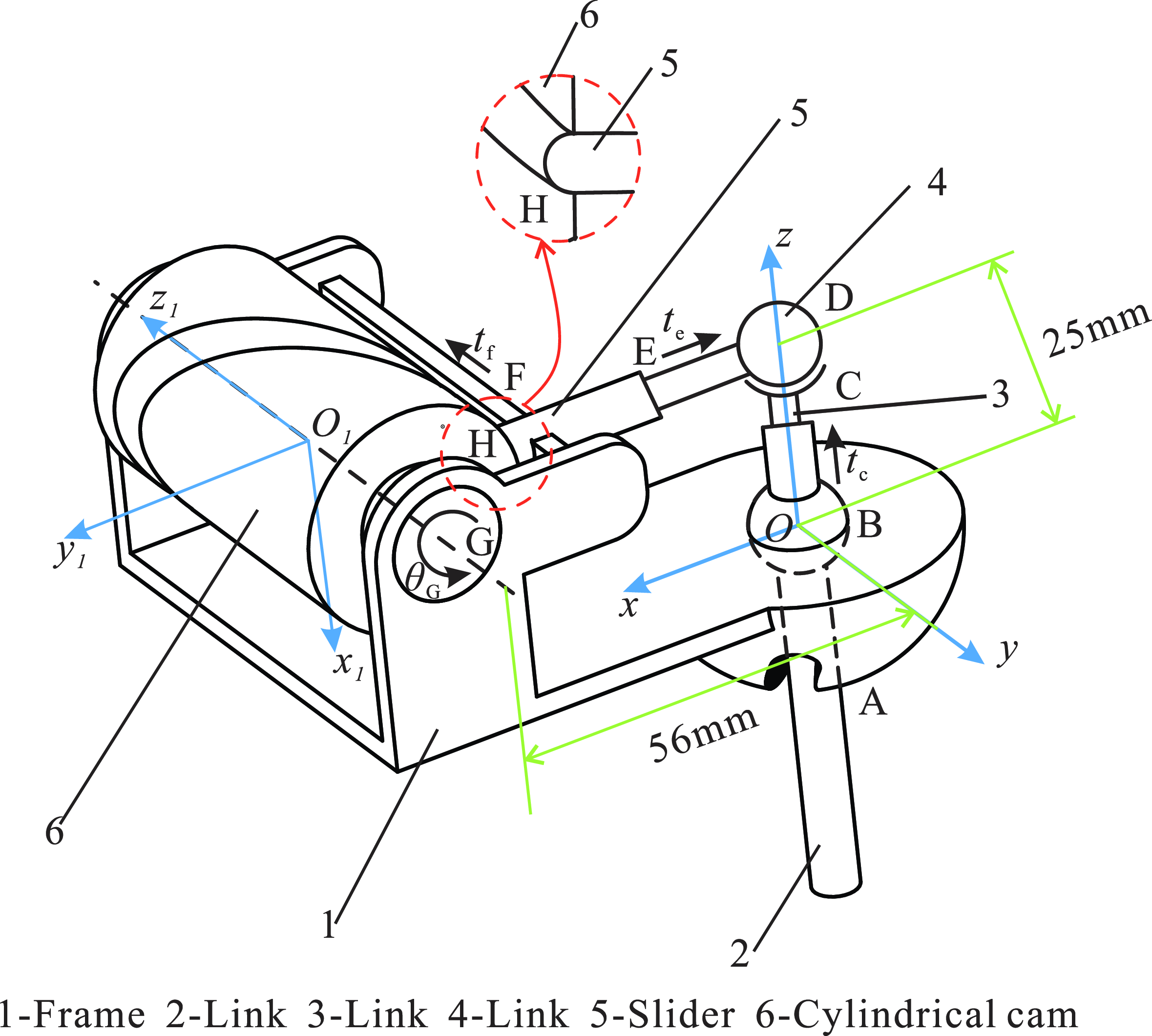
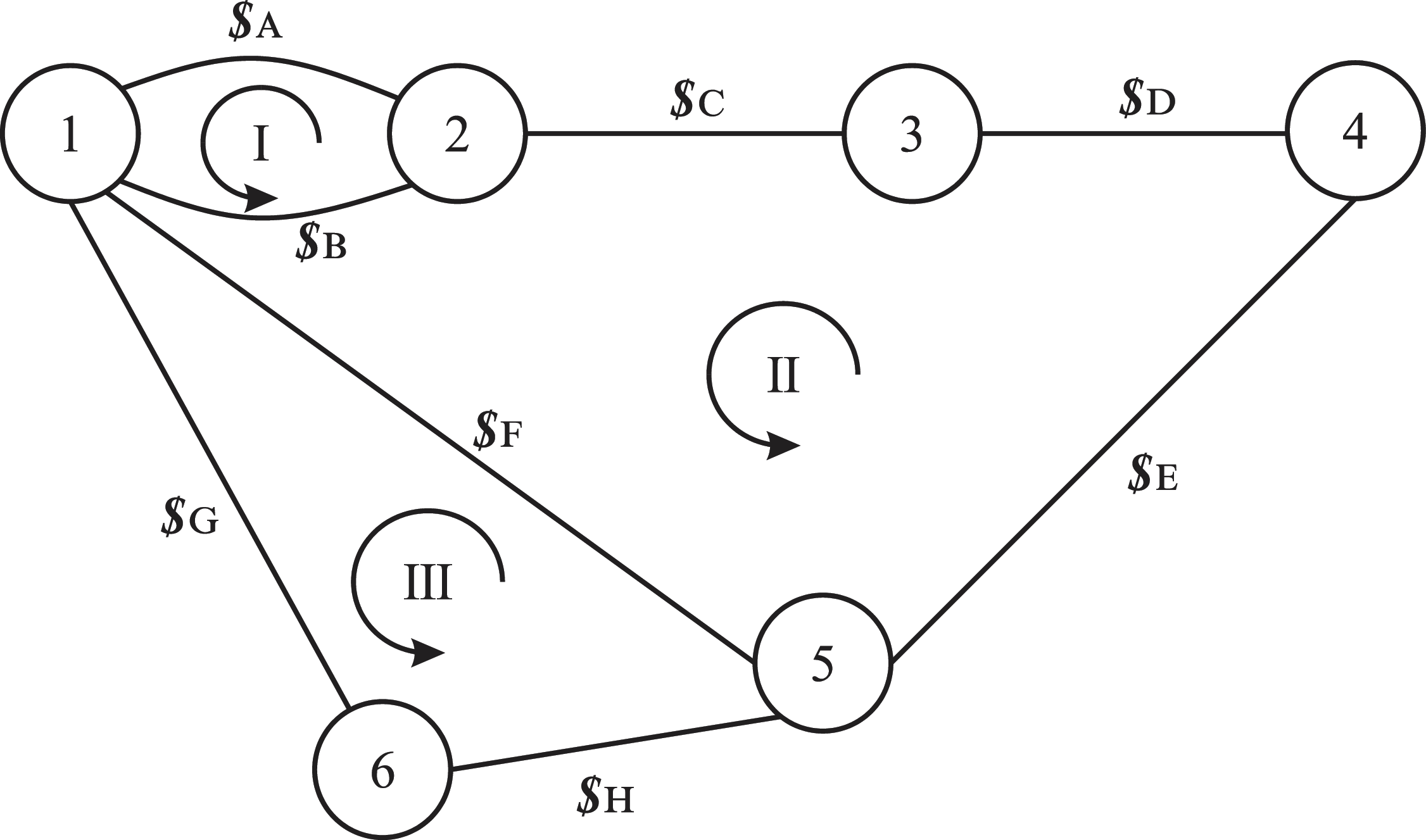
The second example is to analyze a cylindrical cam mechanism as shown in Figure 8, where the cylindrical cam component rotates about the frame with revolute A, directing along the y-axis. The vertical distance between axis of revolute pair A and y-axis is 112.5 mm. The cam component and its follower form a HKP B, whose trajectory can be expressed by parametric equation under the trajectory coordinate system
 $O_{\mathrm{T}}-x_{\mathrm{T}}y_{\mathrm{T}}z_{\mathrm{T}}, \left\{\begin{array}{l} x=40\sin t\\ y=-30\sin 2t\\ z=40\cos t \end{array}\right.,t\in \left(0,2\pi \right)$
. At the current position, three axes of
 $O_{\mathrm{T}}-x_{\mathrm{T}}y_{\mathrm{T}}z_{\mathrm{T}}$
are parallel to the corresponding axes of the global coordinate system
 $O-xyz$
. The follower translates along the y-axis with prismatic pair C. The vertical distance between axis of prismatic pair C and y-axis is 40 mm.
Cylindrical cam mechanism.

(1) DOF analysis of the mechanism by the G-K formula
In 3D space, the G-K formula for calculating the DOF is
 \begin{equation} m_{\mathrm{G}}=6n-5P_{5}-4P_{4}-3P_{3}-2P_{2}-P_{1} \end{equation}
where m G represen,ts the DOF of the spatial mechanism. n is the number of moving components in the mechanism. P 5, P 4, P 3, P 2 and P 1 represent the numbers of fifth-class pairs, fourth-class pairs, third-class pairs, second-class pairs, and first-class pairs, respectively.
Therefore, the DOF of this mechanism can be obtained,
 \begin{align} \begin{array}{c} m_{\mathrm{G}}=6n-5P_{5}-4P_{4}-3P_{3}-2P_{2}-P_{1}\\[10pt] =6\times 2-5\times 2-2\times 1=0 \end{array} \end{align}
The computational result from the G-K formula conflicts with the simulation verification, which shows that this mechanism is movable, so the G-K formula fails into error for this mechanism.
(2) DOF analysis of the mechanism by the instantaneous screw theory
At this movement, the parameter of the corresponding trajectory equation is t = 0. Therefore, the positions of points A and B are
 $\boldsymbol{A}=(\begin{array}{l@{\quad}l@{\quad}l} 0 & 75 & 112.5 \end{array})^{\mathrm{T }}, \boldsymbol{B}=(\begin{array}{l@{\quad}l@{\quad}l} 0 & 0 & 72.5 \end{array})^{\mathrm{T }}$
.
The direction vectors of revolute pair A is
 $\boldsymbol{s}_{\mathrm{A}}=[\begin{array}{l@{\quad}l@{\quad}l} 0 & 1 & 0 \end{array}]^{\mathrm{T }}$
, the direction vectors of the three axes of the
 $O_{\mathrm{T}}-x_{\mathrm{T}}y_{\mathrm{T}}z_{\mathrm{T}}$
are, respectively,
 $\boldsymbol{s}_{\mathrm{xt}}=(\begin{array}{l@{\quad}l@{\quad}l} 1 & 0 & 0 \end{array})^{\mathrm{T }}, \boldsymbol{s}_{\mathrm{yt}}=(\begin{array}{l@{\quad}l@{\quad}l} 0 & 1 & 0 \end{array})^{\mathrm{T }}, \boldsymbol{s}_{\mathrm{zt}}=(\begin{array}{l@{\quad}l@{\quad}l} 0 & 0 & 1 \end{array})^{\mathrm{T }}$
. The rotation around the contact point B of the higher kinematic pair can be regarded as a spherical pair, its three direction vectors are, respectively,
 $\boldsymbol{s}_{\mathrm{x}}=(\begin{array}{l@{\quad}l@{\quad}l} 1 & 0 & 0 \end{array})^{\mathrm{T }}, \boldsymbol{s}_{\mathrm{y}}=(\begin{array}{l@{\quad}l@{\quad}l} 0 & 1 & 0 \end{array})^{\mathrm{T }}, \boldsymbol{s}_{\mathrm{z}}=(\begin{array}{l@{\quad}l@{\quad}l} 0 & 0 & 1 \end{array})^{\mathrm{T }}$
. The direction vector of the prismatic pair C is
 $\boldsymbol{s}_{\mathrm{C}}=(\begin{array}{l@{\quad}l@{\quad}l} 0 & 1 & 0 \end{array})^{\mathrm{T }}$
.
Therefore, the screws of each kinematic pair can be written as
 \begin{equation} \begin{array}{l} \boldsymbol{\$} _{\mathrm{A}}=\left(\begin{array}{c} \boldsymbol{s}_{a}\\ A\times \boldsymbol{s}_{a} \end{array}\right)\mathrm{,}\ \boldsymbol{\$} _{\mathrm{xt}}=\left(\begin{array}{c} \mathbf{0}\\ \boldsymbol{s}_{\mathrm{xt}} \end{array}\right)\mathrm{,}\ \boldsymbol{\$} _{\mathrm{yt}}=\left(\begin{array}{c} \mathbf{0}\\ \boldsymbol{s}_{\mathrm{yt}} \end{array}\right)\mathrm{,}\ \boldsymbol{\$} _{\mathrm{zt}}=\left(\begin{array}{c} \mathbf{0}\\ \boldsymbol{s}_{\mathrm{zt}} \end{array}\right)\\ [15pt] \boldsymbol{\$} _{\mathrm{C}}=\left(\begin{array}{c} \mathbf{0}\\ \boldsymbol{s}_{\mathrm{c}} \end{array}\right)\mathrm{,}\ \boldsymbol{\$} _{\mathrm{x}}=\left(\begin{array}{c} \boldsymbol{s}_{\mathrm{x}}\\ \boldsymbol{B}\times \boldsymbol{s}_{\mathrm{x}} \end{array}\right)\mathrm{,}\ \boldsymbol{\$} _{\mathrm{y}}=\left(\begin{array}{c} \boldsymbol{s}_{\mathrm{y}}\\ \boldsymbol{B}\times \boldsymbol{s}_{\mathrm{y}} \end{array}\right)\mathrm{,}\ \boldsymbol{\$} _{\mathrm{z}}=\left(\begin{array}{c} \boldsymbol{s}_{\mathrm{z}}\\ \boldsymbol{B}\times \boldsymbol{s}_{\mathrm{z}} \end{array}\right) \end{array} \end{equation}
The velocity ratio of movement along the coordinate
 $x_{\mathrm{T}}\mathrm{-axis}$
and
 $y_{\mathrm{T}}\mathrm{-axis}$
is
 $R_{\mathrm{a}}=\dfrac{\boldsymbol{v}_{\mathrm{yt}}}{\boldsymbol{v}_{\mathrm{xt}}}=\dfrac{dy}{dx}=\dfrac{dy/dt}{dx/dt}=\dfrac{-60\cos \left(0\right)}{40\cos \left(0\right)}=-1.5$
, and the velocity ratio of movement along the coordinate
 $x_{\mathrm{T}}\mathrm{-axis}$
and
 $z_{\mathrm{T}}\mathrm{-axis}$
is
 $R_{\mathrm{b}}=\dfrac{\boldsymbol{v}_{\mathrm{zt}}}{\boldsymbol{v}_{\mathrm{xt}}}=\dfrac{dz}{dx}=\dfrac{dz/dt}{dx/dt}=\dfrac{-40\sin \left(0\right)}{40\cos \left(0\right)}=0$
.
Therefore, its constraint matrix be obtained as
 \begin{equation} \boldsymbol{M}_{{\mathrm{h}_{8\times 8}}}=\left(\begin{array}{l@{\quad}l@{\quad}l@{\quad}l@{\quad}l@{\quad}l@{\quad}l@{\quad}l} \boldsymbol{\$} _{\mathrm{A}} & \boldsymbol{\$} _{xt} & \boldsymbol{\$} _{\mathrm{yt}} & \boldsymbol{\$} _{\mathrm{zt}} & \boldsymbol{\$} _{\mathrm{x}} & \boldsymbol{\$} _{\mathrm{y}} & \boldsymbol{\$} _{\mathrm{z}} & \boldsymbol{\$} _{\mathrm{C}}\\ 0 & R_{\mathrm{a}} & -1 & 0 & 0 & 0 & 0 & 0\\ 0 & R_{\mathrm{b}} & 0 & -1 & 0 & 0 & 0 & 0 \end{array}\right) \end{equation}
Use MATLAB to find its rank, and the constraint matrix is an
 $8\times 8$
matrix. Therefore, the degree of freedom of this higher kinematic pair mechanism can be obtained as
 \begin{equation} m_{\mathrm{h}}=n_{\mathrm{h}}-\text{rank} \! \left(\boldsymbol{M}_{{\mathrm{h}_{8\times 8}}}\right)=8-7=1 \end{equation}
The DOF calculated by the proposed method has been validated through the technique of CAD in Solidworks too.
(3) Analysis of kinematic relationship between the motion angles by the finite screw theory
Figure 8 shows the initial configuration of the mechanism, and the linear as well as angular displacements are all assumed to be zero.
Therefore, the finite screws of each kinematic pair are
 \begin{align} \boldsymbol{S}_{\mathrm{A}} & = 2\tan \frac{\theta _{\mathrm{A}}}{2}\left(\begin{array}{c} \boldsymbol{s}_{\mathrm{A}}\\ \boldsymbol{A}\times \boldsymbol{s}_{\mathrm{A}} \end{array}\right)\mathrm{,}\ \boldsymbol{S}_{\mathrm{C}}=t_{\mathrm{c}}\left(\begin{array}{c} \mathbf{0}\\ \boldsymbol{s}_{\mathrm{C}} \end{array}\right) \nonumber \\[10pt] \boldsymbol{S}_{\mathrm{h}} & = 2\tan \dfrac{\theta _{\mathrm{z}}}{2}\left(\begin{array}{c} \boldsymbol{s}_{\mathrm{z}}\\ \boldsymbol{B}\times \boldsymbol{s}_{\mathrm{z}} \end{array}\right){\unicode[Arial]{x0394}} 2\tan \dfrac{\theta _{\mathrm{y}}}{2}\left(\begin{array}{c} \boldsymbol{s}_{\mathrm{y}}\\ \boldsymbol{B}\times \boldsymbol{s}_{\mathrm{y}} \end{array}\right){\unicode[Arial]{x0394}} 2\tan \dfrac{\theta _{\mathrm{x}}}{2}\left(\begin{array}{c} \boldsymbol{s}_{\mathrm{x}}\\ \boldsymbol{B}\times \boldsymbol{s}_{\mathrm{x}} \end{array}\right) \nonumber \\ & \quad {\unicode[Arial]{x0394}} t_{\mathrm{xt}}\left(\begin{array}{c} \mathbf{0}\\ \boldsymbol{s}_{\mathrm{xt}} \end{array}\right){\unicode[Arial]{x0394}} t_{\mathrm{yt}}\left(\begin{array}{c} \mathbf{0}\\ \boldsymbol{s}_{\mathrm{yt}} \end{array}\right){\unicode[Arial]{x0394}} t_{\mathrm{zt}}\left(\begin{array}{c} \mathbf{0}\\ \boldsymbol{s}_{\mathrm{zt}} \end{array}\right) \end{align}
where
 $\left\{\begin{array}{l} t_{\mathrm{x}}=40\sin t\\ t_{\mathrm{y}}=-30\sin 2t\\ t_{\mathrm{z}}=40+40\cos t \end{array}\right.,t\in \left(0,2\pi \right)$
.
Therefore, the finite movement of the mechanism can be written as
 \begin{equation} \boldsymbol{S}=-\boldsymbol{S}_{\boldsymbol{C}}{\unicode[Arial]{x0394}} \boldsymbol{S}_{\boldsymbol{h}}{\unicode[Arial]{x0394}} \boldsymbol{S}_{\boldsymbol{A}}=\mathbf{0}. \end{equation}
Since the axis of the prismatic pair C is parallel to the axis of the revolute pair A,
 $\theta _{\mathrm{x}}=0,\theta _{\mathrm{z}}=0,\theta _{\mathrm{y}}=-\theta _{\mathrm{A}}$
. We assume that when the z
T-axis is parallel to the z-axis,
 $\theta _{a}=0$
, and the cylindrical cam stops after rotating one revolution around the y
T-axis. From the Eq. (41), the relationship diagram between
 $\theta _{\mathrm{a}}$
and
 $t_{\mathrm{c}}$
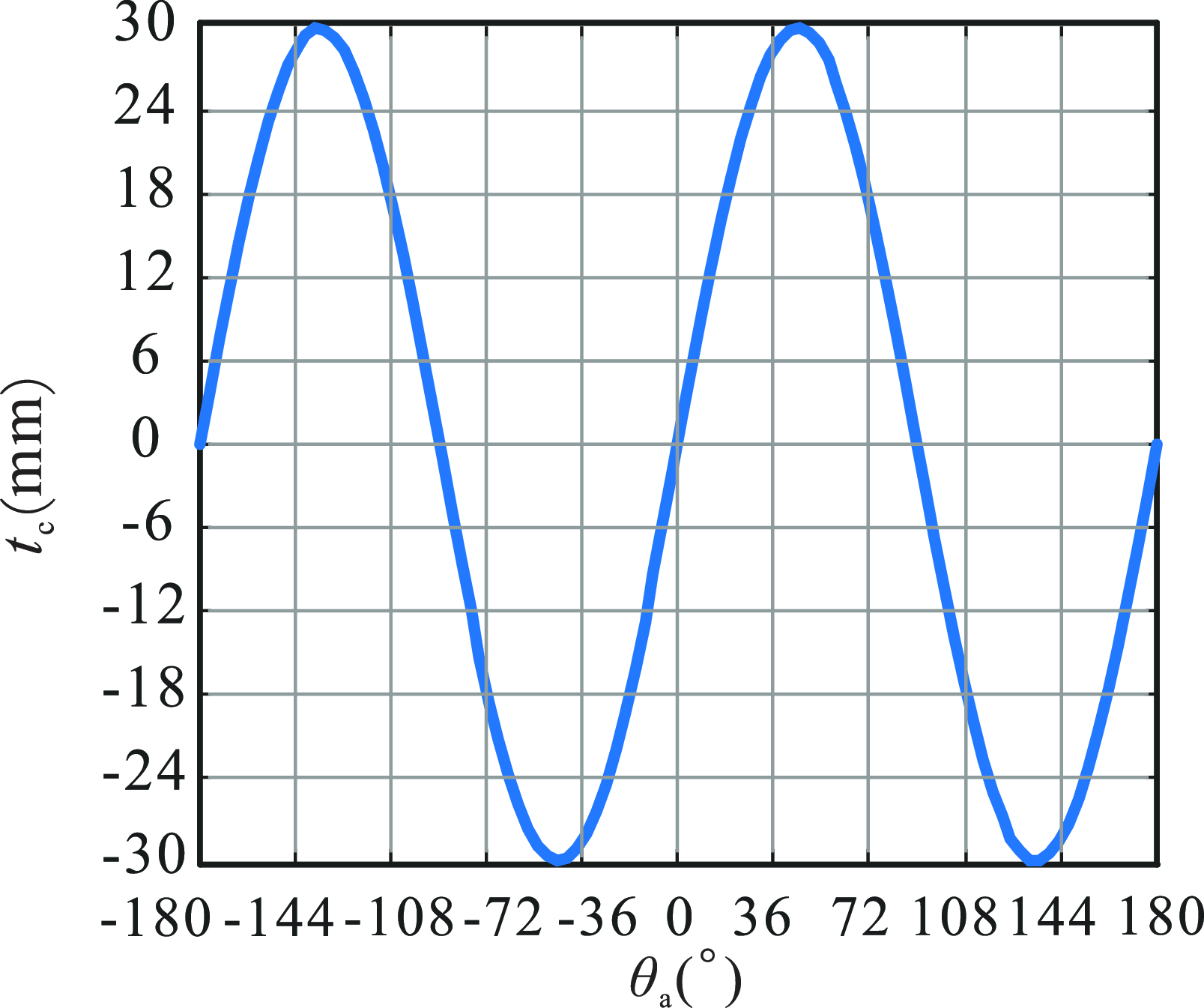
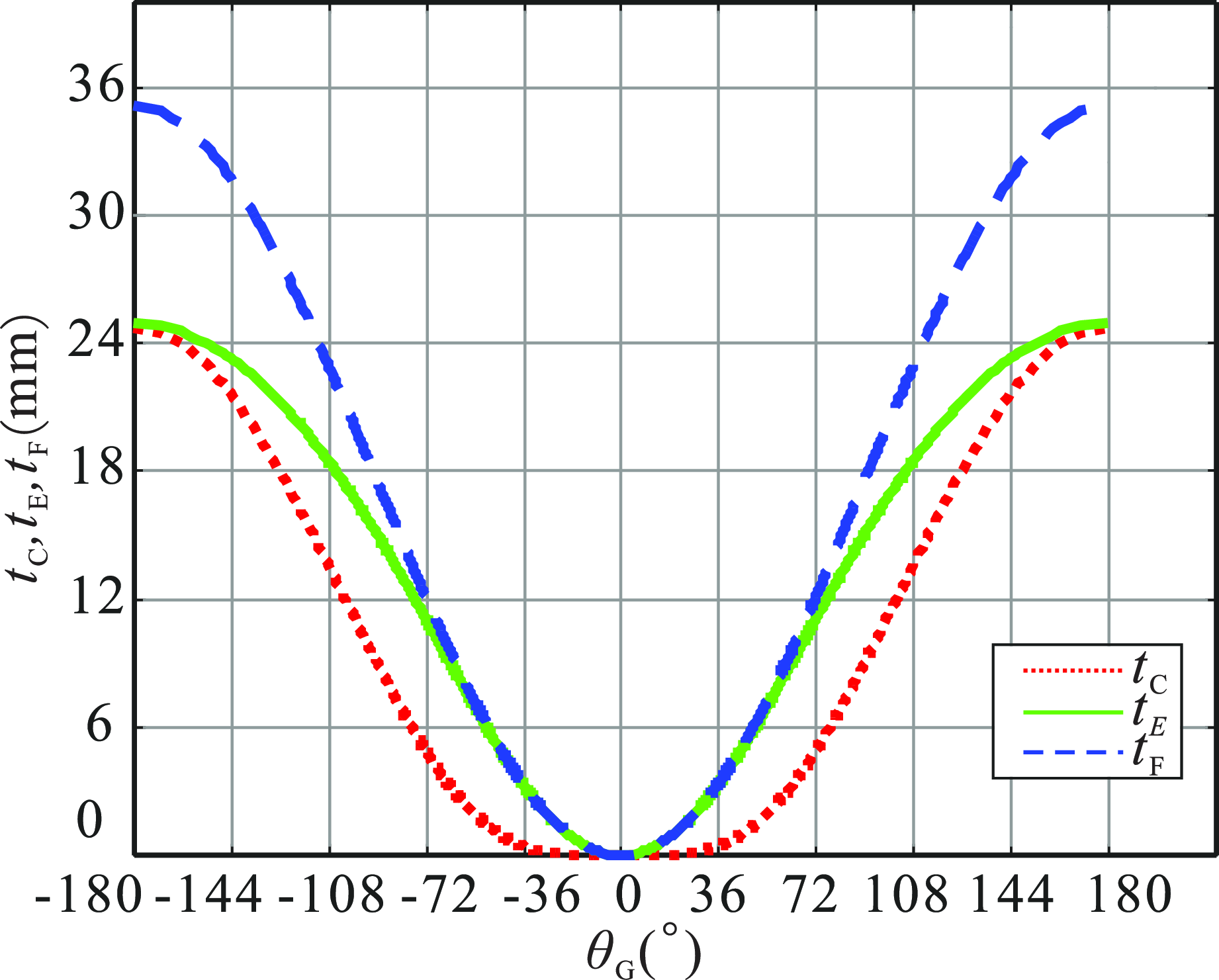
can be obtained, as shown in Figure 9. The rotation of the cylindrical cam drives the slider C to make reciprocating motion.
The relationship between cam rotation angle
 $\theta _{a}$
and displacement of prismatic pair
 $t_{c}$
.

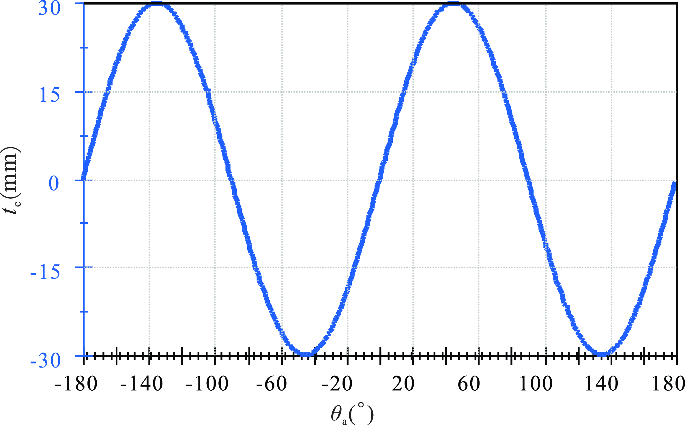
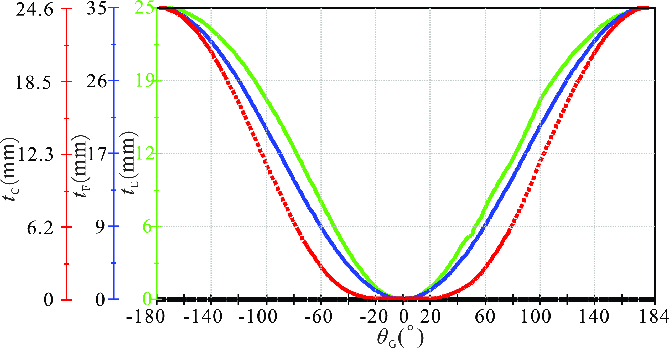
The motion simulation of the cylindrical cam mechanism was conducted using the motion module, and the resulting graphical analysis as shown in Figure 10. By comparing Figure 9 and Figure 10, it reveals perfect alignment between the simulation results and that using the proposed one.
The simulation results of cylindrical cam mechanism.

4.3. Higher kinematic pair parallel mechanism
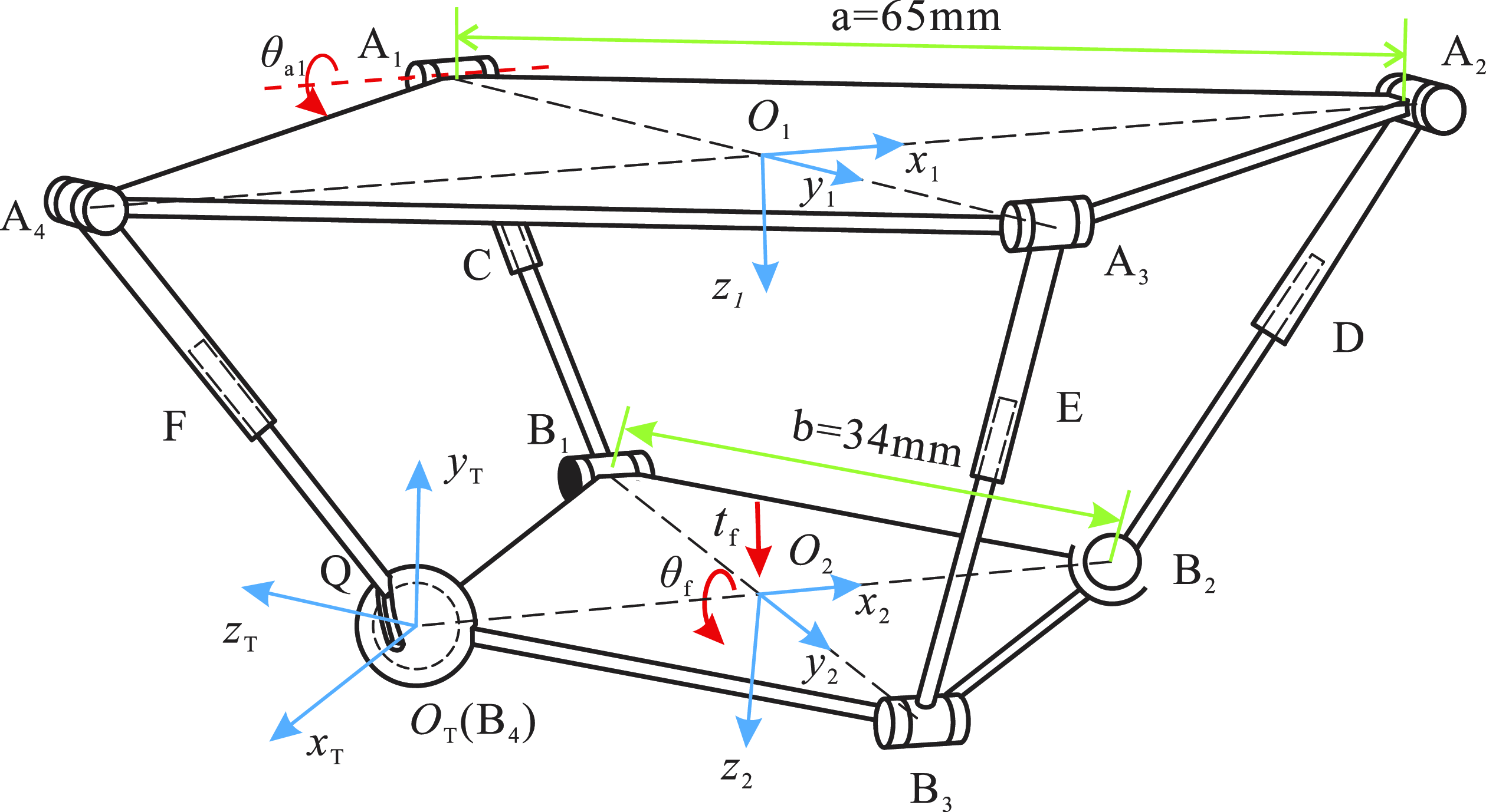
The third case is to analyze a genearal spatial mchanism, as shown in Figure 11, it is a parallel mechanism with a higher kinematic pair (HKP). This spatial 2RPR-1RPS-1RPSHKP mechanism have a static platform A1A2A3A4, a moving platform B1B2B3B4, and four branches. Side length of the static platform is
 $a=65\mathrm{mm}$
. Side length of the moving platform is
 $b=34\mathrm{mm}$
. Points
 $\mathrm{A}_{1}, \mathrm{A}_{2}, \mathrm{A}_{3}, \mathrm{A}_{4}, \mathrm{B}_{1}$
, and
 $\mathrm{B}_{2}$
are all revolute pairs. Points C, D, E, and F are all prismatic pair. Point
 $\mathrm{B}_{3}$
and Point
 $\mathrm{B}_{4}$
are spherical pairs. At the point
 $O_{\mathrm{T}}$
, there is a grooved spherical shell, and the spherical shell component and its follower form a HKP Q. The parametric equation of the trajectory of the HKP Q under the
 $O_{\mathrm{T}}-x_{\mathrm{T}}y_{\mathrm{T}}z_{\mathrm{T}}$
is
 $\left\{\begin{array}{l} x=7.5\cos 2t\cos t\\ y=7.5\sin 2t\cos t\\ z=7.5\sin t \end{array}\right.,t\in \left(0,\dfrac{\pi }{2}\right)$
.
 $x_{\mathrm{T}}\mathrm{-axis}$
and
 $y_{\mathrm{T}}\mathrm{-axis}$
are parallel to the square sides of the moving platform. The coordinate system of the static platform is
 $O_{1}-x_{1}y_{1}z_{1}$
, and the coordinate system of the moving platform is
 $O_{2}-x_{2}y_{2}z_{2}$
.
2RPR-1RPS-1RPSHKP mechanism.

(1) DOF analysis of the mechanism by the G-K formula
According to Eq. (35), the DOF of this mechanism can be obtained,
 \begin{align} m_{\mathrm{G}} & =6n-5P_{5}-4P_{4}-3P_{3}-2P_{2}-P_{1}\\\nonumber & =6\times 9-5\times 10-3\times 2-2\times 1=-4 \end{align}
However, after a simulation verification, this result is incorrect.
(2) DOF analysis of the mechanism by the instantaneous screw theory
When the mechanism moves to the position shown in Figure 11, the angle between the static platform and the moving platform is
 $\theta =12.49^{\circ }$
, based on the parametric equation of trajectory, we can obtain
 \begin{equation} \frac{\cos\left(\dfrac{\pi }{4}+{\arctan }\dfrac{x}{z}\right)\sqrt{x^{2}+z^{2}}}{y}=\tan \theta. \end{equation}
Therefore, the parameters of trajectory equations are
 $t\approx 0.5903$
, and the distance from point
 $O_{1}$
to
 $O_{2}$
can be obtained by measurement, it is
 $d=27.96\mathrm{mm}$
. The positions of each point are
 \begin{equation} \begin{array}{l} \boldsymbol{A}_{1}=\left(\begin{array}{l@{\quad}l@{\quad}l} 0 & -\dfrac{\sqrt{2}}{2}a & 0 \end{array}\right)^{\mathrm{T }}\mathrm{,}\ \boldsymbol{A}_{2}=\left(\begin{array}{l@{\quad}l@{\quad}l} \dfrac{\sqrt{2}}{2}a & 0 & 0 \end{array}\right)^{\mathrm{T }}\mathrm{,}\ \boldsymbol{A}_{3}=\left(\begin{array}{l@{\quad}l@{\quad}l} 0 & \dfrac{\sqrt{2}}{2}a & 0 \end{array}\right)^{\mathrm{T }}\mathrm{,}\\ [10pt]\boldsymbol{A}_{4}=\left(\begin{array}{l@{\quad}l@{\quad}l} -\dfrac{\sqrt{2}}{2}a & 0 & 0 \end{array}\right)^{\mathrm{T }}\mathrm{,}\ \boldsymbol{B}_{1}=\left(\begin{array}{l@{\quad}l@{\quad}l} 0 & -\dfrac{\sqrt{2}}{2}b\cos \theta & d-b\sin \theta \end{array}\right)^{\mathrm{T }}\mathrm{,}\ \boldsymbol{B}_{2}=\left(\begin{array}{l@{\quad}l@{\quad}l} b & 0 & d \end{array}\right)^{\mathrm{T }}\mathrm{,}\\ [10pt]\boldsymbol{B}_{3}=\left(\begin{array}{l@{\quad}l@{\quad}l} 0 & \dfrac{\sqrt{2}}{2}b\cos \theta & d+b\sin \theta \end{array}\right)^{\mathrm{T }}\mathrm{,}\ \boldsymbol{B}_{4}=\left(\begin{array}{l@{\quad}l@{\quad}l} -b & 0 & d \end{array}\right)^{\mathrm{T }}\mathrm{,}\ \boldsymbol{O}_{2}=\left(\begin{array}{l@{\quad}l@{\quad}l} 0 & 0 & d \end{array}\right)^{\mathrm{T }} \end{array} \end{equation}
The direction vectors of each revolute pair can be written as
 \begin{equation} \boldsymbol{s}_{\mathrm{A}1}=\boldsymbol{s}_{\mathrm{A}3}=\left(\begin{array}{l@{\quad}l@{\quad}l} 1 & 0 & 0 \end{array}\right)^{\mathrm{T }}\mathrm{,}\ \boldsymbol{s}_{\mathrm{A}2}=\boldsymbol{s}_{\mathrm{A}4}=\left(\begin{array}{l@{\quad}l@{\quad}l} 0 & 1 & 0 \end{array}\right)^{\mathrm{T }}\mathrm{,}\ \boldsymbol{s}_{\mathrm{B}1}=\boldsymbol{s}_{\mathrm{B}3}=\left(\begin{array}{l@{\quad}l@{\quad}l} 1 & 0 & 0 \end{array}\right)^{\mathrm{T }}. \end{equation}
The direction vectors of each prismatic pair can be written as
 \begin{equation} \boldsymbol{s}_{\mathrm{C}}=\left(\frac{\boldsymbol{A}_{\boldsymbol{1}}-\boldsymbol{B}_{\boldsymbol{1}}}{\left| \boldsymbol{A}_{\boldsymbol{1}}-\boldsymbol{B}_{\boldsymbol{1}}\right| }\right)^{\mathrm{T }}\mathrm{,}\ \boldsymbol{s}_{\mathrm{D}}=\left(\frac{\boldsymbol{A}_{\boldsymbol{2}}-\boldsymbol{B}_{\boldsymbol{2}}}{\left| \boldsymbol{A}_{2}-\boldsymbol{B}_{2}\right| }\right)^{\mathrm{T }}\mathrm{,}\ \boldsymbol{s}_{\mathrm{E}}=\left(\frac{\boldsymbol{A}_{\boldsymbol{3}}-\boldsymbol{B}_{\boldsymbol{3}}}{\left| \boldsymbol{A}_{3}-\boldsymbol{B}_{3}\right| }\right)^{\mathrm{T }}\mathrm{,}\ \boldsymbol{s}_{\mathrm{F}}=\left(\frac{\boldsymbol{A}_{\boldsymbol{4}}-\boldsymbol{B}_{4}}{\left| \boldsymbol{A}_{4}-\boldsymbol{B}_{4}\right| }\right)^{\mathrm{T }} .\end{equation}
The direction vectors of the three axes of the
 $O_{\mathrm{T}}-x_{\mathrm{T}}y_{\mathrm{T}}z_{\mathrm{T}}$
are, respectively,
 $\boldsymbol{s}_{\mathrm{xt}}=\left(\frac{\dfrac{\boldsymbol{B}_{4}+\boldsymbol{B}_{3}}{2}-\boldsymbol{O}_{2}}{\left| \dfrac{\boldsymbol{B}_{4}+\boldsymbol{B}_{3}}{2}-\boldsymbol{O}_{2}\right| }\right)^{\mathrm{T }}, \boldsymbol{s}_{\mathrm{zt}}=\left(\frac{\dfrac{\boldsymbol{B}_{1}+\boldsymbol{B}_{4}}{2}-\boldsymbol{O}_{2}}{\left| \dfrac{\boldsymbol{B}_{1}+\boldsymbol{B}_{4}}{2}-\boldsymbol{O}_{2}\right| }\right)^{\mathrm{T }}, \boldsymbol{s}_{\mathrm{yt}}=\boldsymbol{s}_{\mathrm{xt}}\times \boldsymbol{s}_{\mathrm{zt}}$
. The direction vector of the spherical pair is
 $\left\{\begin{array}{c} \boldsymbol{s}_{\mathrm{x}}=\left(\begin{array}{l@{\quad}l@{\quad}l} 1 & 0 & 0 \end{array}\right)^{\mathrm{T }}\\ \boldsymbol{s}_{\mathrm{y}}=\left(\begin{array}{l@{\quad}l@{\quad}l} 0 & 1 & 0 \end{array}\right)^{\mathrm{T }}\\ \boldsymbol{s}_{\mathrm{z}}=\left(\begin{array}{l@{\quad}l@{\quad}l} 0 & 0 & 1 \end{array}\right)^{\mathrm{T }} \end{array}\right.$
.
Therefore, the screws of all revolute pairs and prismatic pairs are
 \begin{equation} \begin{array}{c} \boldsymbol{\$} _{\mathrm{A}1}=\left(\begin{array}{c} \boldsymbol{s}_{\mathrm{A}1}\\ \boldsymbol{A}_{1}\times \boldsymbol{s}_{\mathrm{A}1} \end{array}\right)\mathrm{,}\ \boldsymbol{\$} _{\mathrm{A}2}=\left(\begin{array}{c} \boldsymbol{s}_{\mathrm{A}2}\\ \boldsymbol{A}_{2}\times \boldsymbol{s}_{\mathrm{A}2} \end{array}\right)\mathrm{,}\ \boldsymbol{\$} _{\mathrm{A}3}=\left(\begin{array}{c} \boldsymbol{s}_{\mathrm{A}3}\\ \boldsymbol{A}_{3}\times \boldsymbol{s}_{\mathrm{A}3} \end{array}\right)\mathrm{,}\ \boldsymbol{\$} _{\mathrm{A}4}=\left(\begin{array}{c} \boldsymbol{s}_{\mathrm{A}4}\\ \boldsymbol{A}_{4}\times \boldsymbol{s}_{\boldsymbol{A}4} \end{array}\right)\mathrm{,}\ \boldsymbol{\$} _{\mathrm{B}1}=\left(\begin{array}{c} \boldsymbol{s}_{\mathrm{B}1}\\ \boldsymbol{B}_{\boldsymbol{1}}\times \boldsymbol{s}_{\mathrm{B}1} \end{array}\right)\mathrm{,}\ \\ [10pt]\boldsymbol{\$} _{\mathrm{B}3}=\left(\begin{array}{c} \boldsymbol{s}_{\mathrm{B}3}\\ \boldsymbol{B}_{3}\times \boldsymbol{s}_{\mathrm{B}3} \end{array}\right)\mathrm{,}\ \boldsymbol{\$} _{\mathrm{C}}=\left(\begin{array}{c} \mathbf{0}\\ \boldsymbol{s}_{\mathrm{C}} \end{array}\right)\mathrm{,}\ \boldsymbol{\$} _{\mathrm{D}}=\left(\begin{array}{c} \mathbf{0}\\ \boldsymbol{s}_{\mathrm{D}} \end{array}\right)\mathrm{,}\ \boldsymbol{\$} _{\mathrm{E}}=\left(\begin{array}{c} \mathbf{0}\\ \boldsymbol{s}_{\mathrm{e}} \end{array}\right)\mathrm{,}\ \boldsymbol{\$} _{\mathrm{F}}=\left(\begin{array}{c} \mathbf{0}\\ \boldsymbol{s}_{\mathrm{F}} \end{array}\right) \end{array} .\end{equation}
The screws of spherical pair B2 and spherical pair B4 are
 $\left\{\begin{array}{c} \boldsymbol{\$} _{\mathrm{B}2\mathrm{X}}=\left(\begin{array}{c} \boldsymbol{s}_{\mathrm{x}}\\ \boldsymbol{B}_{\boldsymbol{2}}\times \boldsymbol{s}_{\mathrm{x}} \end{array}\right)\\[10pt] \boldsymbol{\$} _{\mathrm{B}2\mathrm{Y}}=\left(\begin{array}{c} \boldsymbol{s}_{\mathrm{y}}\\ \boldsymbol{B}_{\boldsymbol{2}}\times \boldsymbol{s}_{\mathrm{y}} \end{array}\right)\\[10pt] \boldsymbol{\$} _{\mathrm{B}2\mathrm{Z}}=\left(\begin{array}{c} \boldsymbol{s}_{\mathrm{z}}\\ \boldsymbol{B}_{\boldsymbol{2}}\times \boldsymbol{s}_{\mathrm{z}} \end{array}\right) \end{array}\right., \left\{\begin{array}{c} \boldsymbol{\$} _{\mathrm{B}4\mathrm{X}}=\left(\begin{array}{c} \boldsymbol{s}_{\mathrm{x}}\\ \boldsymbol{B}_{4}\times \boldsymbol{s}_{\mathrm{x}} \end{array}\right)\\[10pt] \boldsymbol{\$} _{\mathrm{B}4\mathrm{Y}}=\left(\begin{array}{c} \boldsymbol{s}_{\mathrm{y}}\\ \boldsymbol{B}_{4}\times \boldsymbol{s}_{\mathrm{y}} \end{array}\right)\\[10pt] \boldsymbol{\$} _{\mathrm{B}4\mathrm{Z}}=\left(\begin{array}{c} \boldsymbol{s}_{\mathrm{z}}\\ \boldsymbol{B}_{4}\times \boldsymbol{s}_{\mathrm{z}} \end{array}\right) \end{array}\right.$
.
The screw of HKP Q is
 $\left\{\begin{array}{c} \boldsymbol{\$} _{\mathrm{xt}}=\left(\begin{array}{c} \boldsymbol{0}\\ \boldsymbol{s}_{\mathrm{xt}} \end{array}\right)\\[10pt] R_{\mathrm{a}}\boldsymbol{\$} _{\mathrm{yt}}=R_{\mathrm{a}}\left(\begin{array}{c} \boldsymbol{0}\\ \boldsymbol{s}_{\mathrm{yt}} \end{array}\right)\\[10pt] R_{\mathrm{b}}\boldsymbol{\$} _{\mathrm{zt}}=R_{\mathrm{b}}\left(\begin{array}{c} \boldsymbol{0}\\ \boldsymbol{s}_{\mathrm{zt}} \end{array}\right)\\[10pt] \boldsymbol{\$} _{\mathrm{x}}=\left(\begin{array}{c} \boldsymbol{s}_{\mathrm{x}}\\ \boldsymbol{A}_{4}\times \boldsymbol{s}_{\mathrm{x}} \end{array}\right)\\ [10pt]\boldsymbol{\$} _{\mathrm{y}}=\left(\begin{array}{c} \boldsymbol{s}_{y}\\ \boldsymbol{A}_{4}\times \boldsymbol{s}_{y} \end{array}\right)\\[10pt] \boldsymbol{\$} _{\mathrm{z}}=\left(\begin{array}{c} \boldsymbol{s}_{z}\\ \boldsymbol{A}_{4}\times \boldsymbol{s}_{\mathrm{z}} \end{array}\right) \end{array}\right.$
.
The velocity ratio of movement along the coordinate
 $x_{T}\mathrm{-axis}$
and
 $y_{T}\mathrm{-axis}$
is
 $R_{\mathrm{a}}=\dfrac{\boldsymbol{v}_{\mathrm{yt}}}{\boldsymbol{v}_{\mathrm{xt}}}=\dfrac{dy}{dx}=\dfrac{dy/dt}{dx/dt}\approx -0.0562$
, and the velocity ratio of movement along the coordinate
 $x_{T}\mathrm{-axis}$
and
 $z_{T}\mathrm{-axis}$
is
 $R_{\mathrm{b}}=\dfrac{\boldsymbol{v}_{\mathrm{zt}}}{\boldsymbol{v}_{\mathrm{xt}}}=\dfrac{dz}{dx}=\dfrac{dz/dt}{dx/dt}\approx -0.4744$
.
Therefore, its constraint matrix can be obtained as
 \begin{equation} \begin{array}{c} \boldsymbol{M}_{{\mathrm{h}_{26\times 22}}}=\left(\begin{array}{l@{\quad}l@{\quad}l@{\quad}l@{\quad}l@{\quad}l@{\quad}l@{\quad}l@{\quad}l@{\quad}l@{\quad}l} \boldsymbol{\$} _{\mathrm{B}4\mathrm{X}} & \boldsymbol{\$} _{\mathrm{B}4\mathrm{Y}} & \boldsymbol{\$} _{\mathrm{B}4\mathrm{Z}} & \boldsymbol{\$} _{\mathrm{X}} & \boldsymbol{\$} _{\mathrm{Y}} & \boldsymbol{\$} _{\mathrm{Z}} & \boldsymbol{\$} _{\mathrm{xt}} & \boldsymbol{\$} _{\mathrm{yt}} & \boldsymbol{\$} _{\mathrm{zt}} & Q & Q\\ Q & Q & Q & -\boldsymbol{\$} _{\mathrm{X}} & -\boldsymbol{\$} _{\mathrm{Y}} & -\boldsymbol{\$} _{\mathrm{Z}} & -\boldsymbol{\$} _{\mathrm{xt}} & -\boldsymbol{\$} _{\mathrm{yt}} & -\boldsymbol{\$} _{\mathrm{zt}} & \boldsymbol{\$} _{\mathrm{A}4} & \boldsymbol{\$} _{\mathrm{B}3}\\ -\boldsymbol{\$} _{\mathrm{B}4\mathrm{X}} & -\boldsymbol{\$} _{\mathrm{B}4\mathrm{Y}} & -\boldsymbol{\$} _{\mathrm{B}4\mathrm{Z}} & Q & Q & Q & Q & Q & Q & -\boldsymbol{\$} _{\mathrm{A}4} & Q\\ Q & Q & Q & Q & Q & Q & Q & Q & Q & Q & Q\\ 0 & 0 & 0 & 0 & 0 & 0 & R_{\mathrm{a}} & -1 & 0 & 0 & 0\\ 0 & 0 & 0 & 0 & 0 & 0 & R_{\mathrm{b}} & 0 & -1 & 0 & 0 \end{array}\cdots \right.\\[20pt] \qquad\qquad\qquad\left.\begin{array}{l@{\quad}l@{\quad}l@{\quad}l@{\quad}l@{\quad}l@{\quad}l@{\quad}l@{\quad}l@{\quad}l@{\quad}l} Q & Q & Q & Q & Q & Q & Q & Q & Q & Q & Q\\ \boldsymbol{\$} _{\mathrm{A}3} & \boldsymbol{\$} _{\mathrm{F}} & \boldsymbol{\$} _{\mathrm{D}} & Q & Q & Q & Q & Q & Q & Q & Q\\ Q & -\boldsymbol{\$} _{\mathrm{F}} & Q & \boldsymbol{\$} _{\mathrm{A}1} & \boldsymbol{\$} _{\mathrm{B}1} & \boldsymbol{\$} _{\mathrm{C}} & Q & Q & Q & Q & Q\\ Q & Q & Q & -\boldsymbol{\$} _{\mathrm{A}1} & -\boldsymbol{\$} _{\mathrm{B}1} & -\boldsymbol{\$} _{\mathrm{C}} & \boldsymbol{\$} _{\mathrm{A}2} & \boldsymbol{\$} _{\mathrm{E}} & \boldsymbol{\$} _{\mathrm{B}2\mathrm{X}} & \boldsymbol{\$} _{\mathrm{B}2\mathrm{Y}} & \boldsymbol{\$} _{\mathrm{B}2\mathrm{Z}}\\ 0 & 0 & 0 & 0 & 0 & 0 & 0 & 0 & 0 & 0 & 0\\ 0 & 0 & 0 & 0 & 0 & 0 & 0 & 0 & 0 & 0 & 0 \end{array}\right) \end{array} \end{equation}
where
 $\boldsymbol{Q}\boldsymbol{=}(\begin{array}{l@{\quad}l@{\quad}l@{\quad}l@{\quad}l@{\quad}l} 0 & 0 & 0 & 0 & 0 & 0 \end{array})^{\mathrm{T }}$
.
The rank of the
 $\boldsymbol{M}_{{\mathrm{h}_{26\times 22}}}$
is calculated by MATLAB, and the constraint matrix
 $\boldsymbol{M}_{{\mathrm{h}_{26\times 22}}}$
has 22 columns. Therefore, the degree of freedom of this HKP mechanism can be obtained as
 \begin{equation} m_{\mathrm{h}}=n_{\mathrm{h}}-\text{rank} \! \left(\boldsymbol{M}_{{\mathrm{h}_{\mathrm{26}\times \mathrm{22}}}}\right)=23-22=1 \end{equation}
It is validated through the technique of CAD in Solidworks, the DOF calculated by the proposed method is correct.
(3) Analysis of kinematic relationship between the motion angles by the finite screw theory
When the static platform and the moving platform are parallel, the mechanism is in the initial position, and the positions of each point are
 \begin{align} \boldsymbol{A}_{1} & =\left(\begin{array}{l@{\quad}l@{\quad}l} 0 & -\dfrac{\sqrt{2}}{2}a & 0 \end{array}\right)^{\mathrm{T }}\mathrm{,}\ \,\boldsymbol{A}_{2}=\left(\begin{array}{l@{\quad}l@{\quad}l} \dfrac{\sqrt{2}}{2}a & 0 & 0 \end{array}\right)^{\mathrm{T }}\mathrm{,}\ \,\boldsymbol{A}_{3}=\left(\begin{array}{l@{\quad}l@{\quad}l} 0 & \dfrac{\sqrt{2}}{2}a & 0 \end{array}\right)^{\mathrm{T }}\mathrm{,}\ \nonumber \\[5pt] \boldsymbol{A}_{4} & =\left(\begin{array}{l@{\quad}l@{\quad}l} -\dfrac{\sqrt{2}}{2}a & 0 & 0 \end{array}\right)^{\mathrm{T }}\mathrm{,}\ \,\boldsymbol{B}_{1}=\left(\begin{array}{l@{\quad}l@{\quad}l} 0 & -\dfrac{\sqrt{2}}{2}\mathrm{b} & d_{0}-b\sin \theta \end{array}\right)^{\mathrm{T }}\mathrm{,}\ \, \nonumber \\[5pt] \boldsymbol{B}_{3} & = \left(\begin{array}{l@{\quad}l@{\quad}l} 0 & \dfrac{\sqrt{2}}{2}b & d_{0} \end{array}\right)^{\mathrm{T }}\mathrm{,}\ \,\boldsymbol{B}_{2}=\left(\begin{array}{l@{\quad}l@{\quad}l} b & 0 & d_{0} \end{array}\right)^{\mathrm{T }}\mathrm{,}\ \,\boldsymbol{B}_{4}=\left(\begin{array}{l@{\quad}l@{\quad}l} -b & 0 & d_{0} \end{array}\right)^{\mathrm{T }}. \end{align}
where
 $d_{0}$
is the distance between the static platform and the moving platform when they are parallel.
Therefore, the finite screws of all revolute pairs and prismatic pairs are
 \begin{equation} \left\{\begin{array}{c} \boldsymbol{S}_{{\mathrm{A}_{\mathrm{i}}}}=2\tan \dfrac{\theta _{{\mathrm{a}_{\mathrm{i}}}}}{2}\left(\begin{array}{c} \boldsymbol{s}_{{\mathrm{a}_{\mathrm{i}}}}\\ \boldsymbol{A}_{i}\times \boldsymbol{s}_{{\mathrm{a}_{\mathrm{i}}}} \end{array}\right),i=1,2,3,4\\ \boldsymbol{S}_{{\mathrm{B}_{\mathrm{i}}}}=2\tan \dfrac{\theta _{{\mathrm{b}_{\mathrm{i}}}}}{2}\left(\begin{array}{c} \boldsymbol{s}_{{\mathrm{b}_{\mathrm{i}}}}\\ \boldsymbol{B}_{\mathrm{i}}\times \boldsymbol{s}_{{\mathrm{b}_{\mathrm{i}}}} \end{array}\right),i=1,3\\ \boldsymbol{S}_{\mathrm{j}}=t_{\mathrm{j}}\left(\begin{array}{c} \mathbf{0}\\ \boldsymbol{s}_{\mathrm{j}} \end{array}\right),j=C,D,E,F \end{array}\right. .\end{equation}
The finite screws of spherical pair B2 and spherical pair B4 are
 \begin{equation} \boldsymbol{S}_{{\mathrm{B}_{\mathrm{i}}}}=2\tan \frac{\theta _{\mathrm{z},\mathrm{i}}}{2}\left(\begin{array}{c} \boldsymbol{s}_{\mathrm{z}}\\ \boldsymbol{B}_{\mathrm{i}}\times \boldsymbol{s}_{\mathrm{z}} \end{array}\right){\unicode[Arial]{x0394}} 2\tan \frac{\theta _{\mathrm{y},\mathrm{i}}}{2}\left(\begin{array}{c} \boldsymbol{s}_{\mathrm{y}}\\ \boldsymbol{B}_{\mathrm{i}}\times \boldsymbol{s}_{\mathrm{y}} \end{array}\right){\unicode[Arial]{x0394}} 2\tan \frac{\theta _{\mathrm{x},\mathrm{i}}}{2}\left(\begin{array}{c} \boldsymbol{s}_{\mathrm{x}}\\ \boldsymbol{B}_{\mathrm{i}}\times \boldsymbol{s}_{\mathrm{x}} \end{array}\right),i=2,4 .\end{equation}
The finite screw of HKP Q is
 \begin{align} \boldsymbol{S}_{\mathrm{h}} & =2\tan \frac{\theta _{\mathrm{z}}}{2}\left(\begin{array}{c} \boldsymbol{s}_{\mathrm{z}}\\ \boldsymbol{A}_{4}\times \boldsymbol{s}_{\mathrm{z}} \end{array}\right){\unicode[Arial]{x0394}} 2\tan \frac{\theta _{\mathrm{y}}}{2}\left(\begin{array}{c} \boldsymbol{s}_{\mathrm{y}}\\ \boldsymbol{A}_{4}\times \boldsymbol{s}_{\mathrm{y}} \end{array}\right){\unicode[Arial]{x0394}} 2\tan \frac{\theta _{\mathrm{x}}}{2}\left(\begin{array}{c} \boldsymbol{s}_{\mathrm{x}}\\ \boldsymbol{A}_{4}\times \boldsymbol{s}_{\mathrm{x}} \end{array}\right) \nonumber \\ & \quad {\unicode[Arial]{x0394}} t_{\mathrm{xt}}\left(\begin{array}{c} \mathbf{0}\\ \boldsymbol{s}_{\mathrm{xt}} \end{array}\right){\unicode[Arial]{x0394}} t_{\mathrm{yt}}\left(\begin{array}{c} \mathbf{0}\\ \boldsymbol{s}_{\mathrm{yt}} \end{array}\right){\unicode[Arial]{x0394}} t_{\mathrm{zt}}\left(\begin{array}{c} \mathbf{0}\\ \boldsymbol{s}_{\mathrm{zt}} \end{array}\right), \end{align}
where
 $\left\{\begin{array}{l} t_{\mathrm{x}}=7.5\cos 2t\cos t-7.5\cos 2t_{0}\cos t_{0}\\ t_{\mathrm{y}}=7.5\sin 2t\cos t-7.5\sin 2t_{0}\cos t_{0}\\ t_{\mathrm{z}}=7.5\sin t-7.5\sin t_{0} \end{array}\right.,t\in \left(0,\frac{\pi }{2}\right)$
.
The finite screws of each branch chain can be written as
 \begin{align} \boldsymbol{S}_{{\mathrm{f}_{1}}}&=\boldsymbol{S}_{{\mathrm{B}_{1}}}{\unicode[Arial]{x0394}} \boldsymbol{S}_{\mathrm{C}}{\unicode[Arial]{x0394}} \boldsymbol{S}_{{\mathrm{A}_{1}}}\end{align}
 \begin{align} \boldsymbol{S}_{{\mathrm{f}_{2}}}&=\boldsymbol{S}_{{\mathrm{B}_{2}}}{\unicode[Arial]{x0394}} \boldsymbol{S}_{\mathrm{D}}{\unicode[Arial]{x0394}} \boldsymbol{S}_{{\mathrm{A}_{2}}}\end{align}
 \begin{align} \boldsymbol{S}_{{\mathrm{f}_{3}}}&=\boldsymbol{S}_{{\mathrm{B}_{3}}}{\unicode[Arial]{x0394}} \boldsymbol{S}_{\mathrm{E}}{\unicode[Arial]{x0394}} \boldsymbol{S}_{{\mathrm{A}_{3}}}\end{align}
 \begin{align} \boldsymbol{S}_{{\mathrm{f}_{4}}}&=\boldsymbol{S}_{\mathrm{h}}{\unicode[Arial]{x0394}} \boldsymbol{S}_{{\mathrm{B}_{4}}}{\unicode[Arial]{x0394}} \boldsymbol{S}_{\mathrm{F}}{\unicode[Arial]{x0394}} \boldsymbol{S}_{{\mathrm{A}_{4}}}\end{align}
where
 $\boldsymbol{S}_{{\mathrm{f}_{\mathrm{i}}}}$
is the finite screw of each branch chain.
The motion of the moving platform in the parallel mechanism is a subset of the motion of the branch chains and satisfies the intersection operation of multiple branch chains [Reference Sun, Yang and Lian35]. Therefore, the finite motion of the moving platform can be obtained as
 \begin{equation} \boldsymbol{S}_{\mathrm{f}}=\boldsymbol{S}_{{\mathrm{f}_{1}}}\cap \boldsymbol{S}_{{\mathrm{f}_{2}}}\cap \boldsymbol{S}_{{\mathrm{f}_{3}}}\cap \boldsymbol{S}_{{\mathrm{f}_{4}}}=2\tan \frac{\theta _{\mathrm{f}}}{2}\left(\begin{array}{c} \boldsymbol{s}_{\mathrm{x}}\\ \boldsymbol{B}_{2}\times \boldsymbol{s}_{\mathrm{x}} \end{array}\right){\unicode[Arial]{x0394}} t_{\mathrm{f}}\left(\begin{array}{c} \mathbf{0}\\ \boldsymbol{s}_{\mathrm{z}} \end{array}\right) .\end{equation}
Therein,
 $\theta _{\mathrm{f}}$
is the angle that the moving platform rotates around the
 $x_{2}\mathrm{-axis}$
, and
 $t_{\mathrm{f}}$
is the distance that the moving platform translates along the
 $z_{1}\mathrm{-axis}$
.
We assume that when the moving platform is parallel to the stationary platform, the mechanism is at the initial position, that is,
 $\theta _{\mathrm{f}}=0^{\circ}$
, when the revolute pair B1 interferes with the static platform, the mechanism will no longer move. Therefore, in this paper, we assume that
 $\theta _{\mathrm{f}}=89^{\circ }$
is the end position of the mechanism.
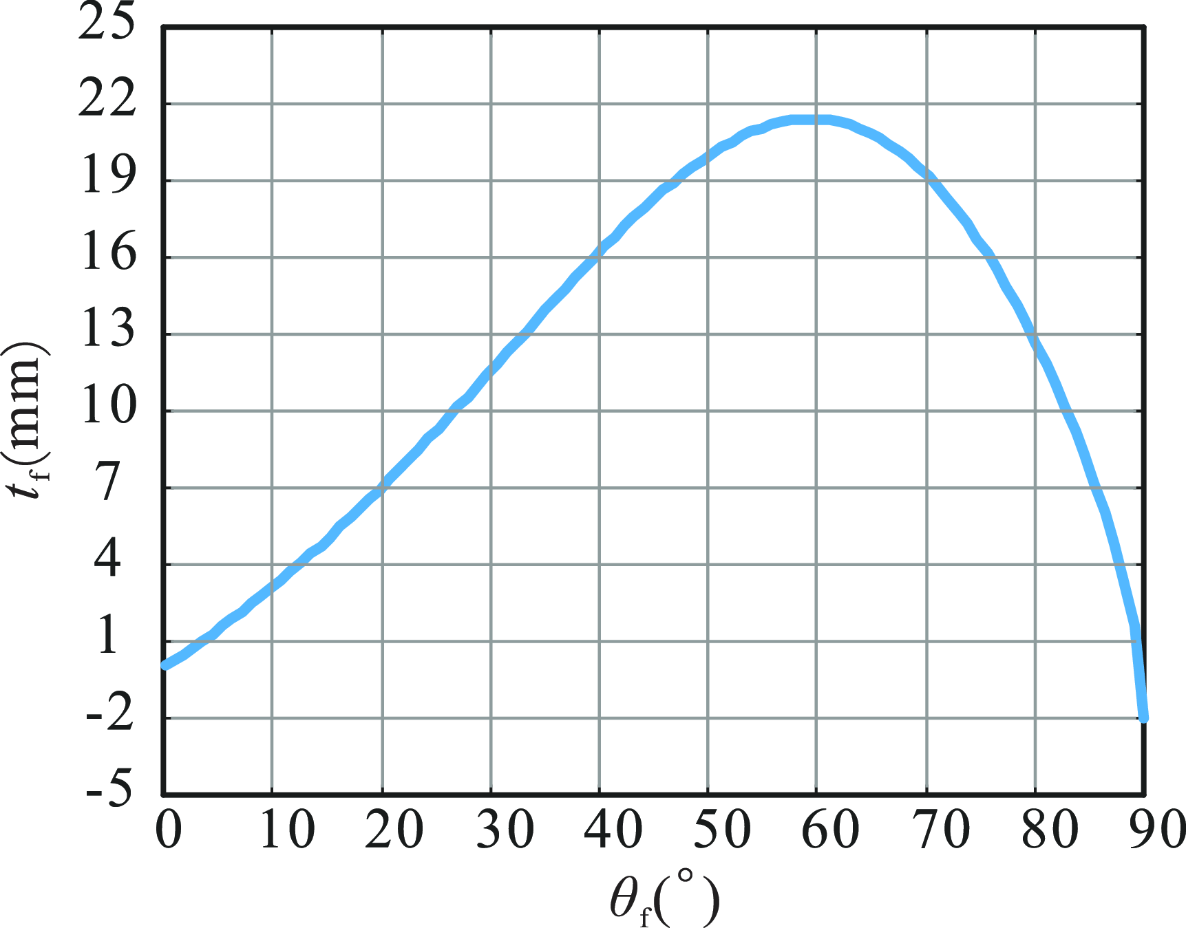
From the above proof, it can be known that the degree of freedom of the moving platform is 1 and combined with the geometric relationship and the trajectory of the HKP, the relationship diagram between
 $\theta _{\mathrm{f}}$
and
 $t_{\mathrm{f}}$
can be obtained, as shown in Figure 12.
The relationship between
 $\theta _{f}$
and
 $t_{f}$
.

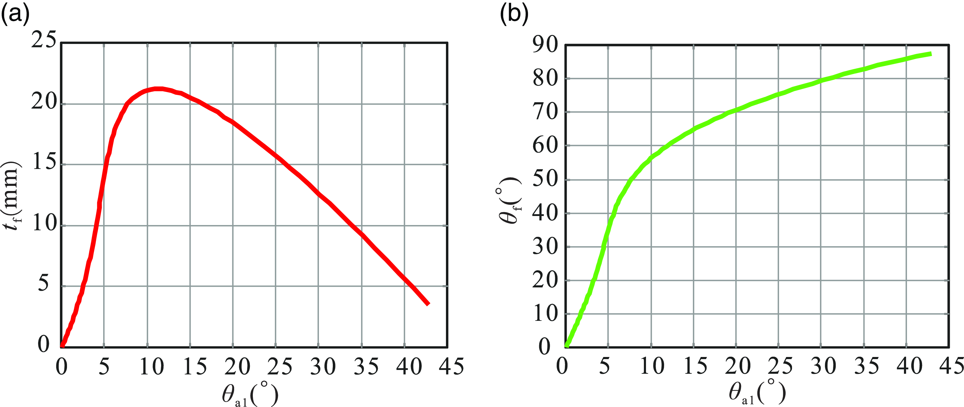
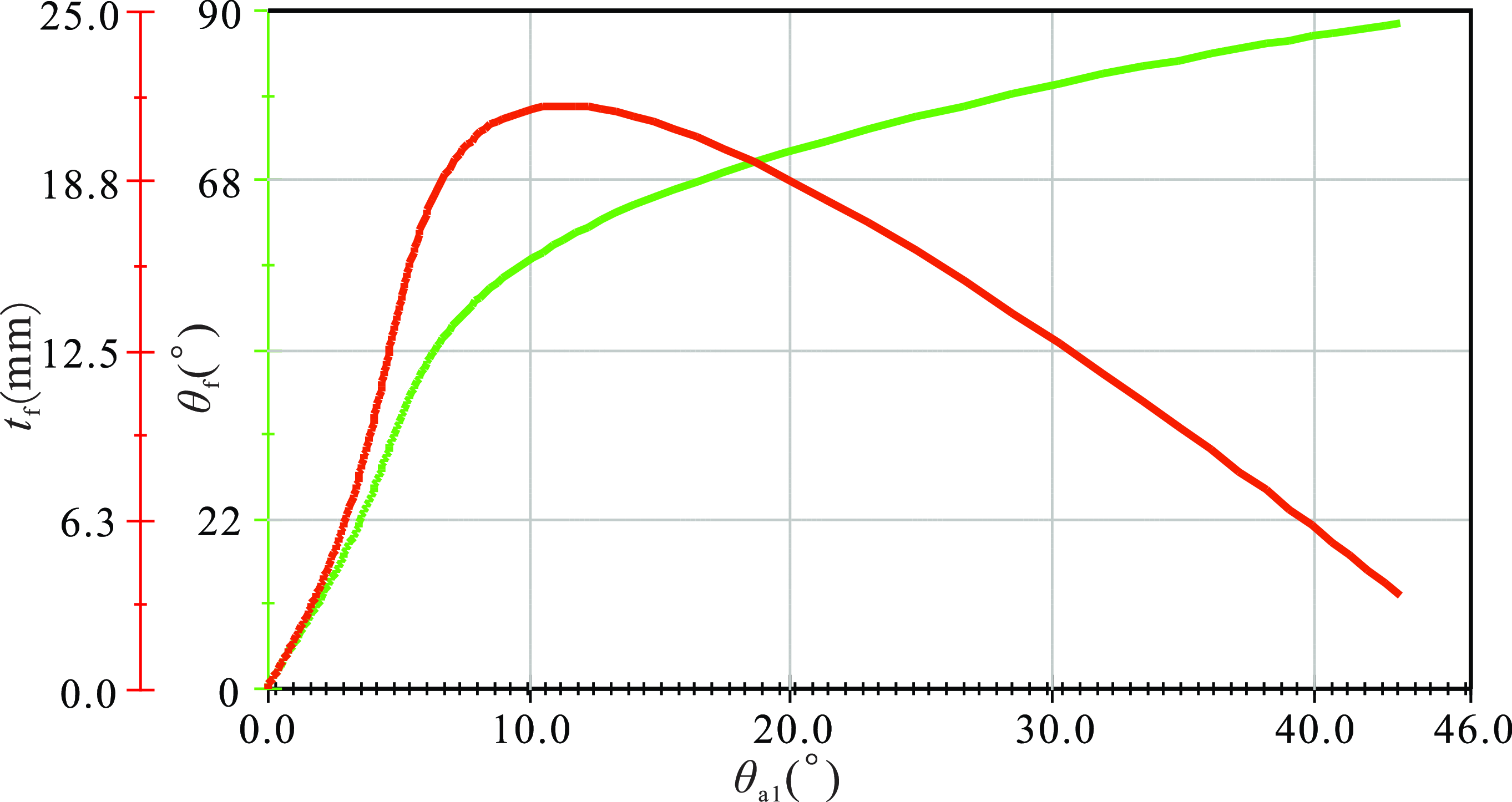
To obtain the kinematical relationship between revolute pair A1 and the moving platform, we can combine the finite motion of branch chains 1 and the finite motion of moving platform.
 \begin{equation} \boldsymbol{S}_{{\mathrm{f}_{1}}} = \boldsymbol{S}_{{\mathrm{B}_{1}}}{\unicode[Arial]{x0394}} \boldsymbol{S}_{\mathrm{C}}{\unicode[Arial]{x0394}} \boldsymbol{S}_{{\mathrm{A}_{1}}}=2\tan \frac{\theta _{\mathrm{f}}}{2}\left(\begin{array}{c} \boldsymbol{s}_{\mathrm{x}}\\ \boldsymbol{B}_{2}\times \boldsymbol{s}_{\mathrm{x}} \end{array}\right){\unicode[Arial]{x0394}} t_{\mathrm{f}}\left(\begin{array}{c} \mathbf{0}\\ \boldsymbol{s}_{\mathrm{z}} \end{array}\right) \end{equation}
According to Eq. (54), the relationship between the rotation angle of revolute pair A1 and the rotation angle
 $\theta _{\mathrm{f}}$
and displacement
 $t_{\mathrm{f}}$
of the moving platform can be calculated can be calculated by MATLAB, respectively, as shown in Figure 12.
As can be seen from Figure 13, the rotation directions of
 $\theta _{\mathrm{a}1}$
and
 $\theta _{\mathrm{f}}$
are opposite, but in order to better represent the kinematic relationships of each kinematic pair here,
 $\theta _{\mathrm{a}1}$
only represents the magnitude of the angle. The rotation of the revolute pair A1 drives the moving platform to rotate around
 $x_{2}\mathrm{-axis}$
and move along
 $z_{1}\mathrm{-axis}$
. The graphical result for the parallel mechanism by the motion simulation, which is presented in Figure 14, matches with the result from the proposed method, see Figure 13.
The kinematical relationship between revolute pair A1 and the moving platform. (a) The relationship between
 $\theta _{\mathrm{a}1}$
and
 $t_{\mathrm{f}}$
. (b) The relationship between
 $\theta _{\mathrm{a}1}$
and
 $\theta _{\mathrm{f}}$
.

The simulation results of parallel mechanism.

4.4. A hybrid mechanism with different types of higher kinematic pairs
The final example is a hybrid mechanism with a cylindrical cam and a ball cam, as shown in Figure 15. Among them, the coordinate system O-xyz is rigidly fixed to the frame, and the coordinate system O
1-x
1
y
1
z
1 is rigidly fixed to the cylindrical cam 6. The kinematic pairs A and H are HKPs. The trace equation of higher trajectory pair A under the coordinate system O-xyz is defined as
 $\left\{\begin{array}{l} x=20\sin t\cos t\\ y=20\cos t\\ z=-20\sin ^{2}t \end{array}\right.,t\in \left(\dfrac{\pi }{4},\dfrac{\pi }{2}\right)$
, while the trace equation of HKP H under the coordinate system O
1-x
1
y
1
z
1 is expressed as
 $\left\{\begin{array}{l} x_{1}=15\sin t_{1}\\ y_{1}=15\cos t_{1}\\ z_{1}=17.5\cos t_{1} \end{array}\right.,t_{1}\in \left(0,2\pi \right)$
. In the position illustrated in the figure, link 2 is parallel to the z-axis. At this configuration, the parameter t of the trace equation for the HKP A corresponds to
 $t=\dfrac{\pi }{2}$
, while the parameter t
1 of the trace equation for the HKP H corresponds to
 $t_{1}=\pi$
. Kinematic pairs B and D are spherical pair. Kinematic pairs C, E, and F are prismatic pair, where the axis of prismatic pair E is parallel to the x-axis, the axis of prismatic pair F is parallel to the y-axis, and the axis of prismatic pair C varies with the motion of the mechanism. Revolute pair G has its rotation axis parallel to the y-axis.
Hybrid mechanism.

(1) DOF analysis of the mechanism by the G-K formula
According to Eq. (35), the DOF of this mechanism can be obtained,
 \begin{equation} \begin{array}{c} m_{\mathrm{G}}=6n-5P_{5}-4P_{4}-3P_{3}-2P_{2}-P_{1}\\ =6\times 5-5\times 4-3\times 2-2\times 2=0 \end{array} \end{equation}
However, after simulation verification, similar to examples 2 and 3, the result is incorrect.
(2) DOF analysis of the mechanism by the instantaneous screw theory
As mentioned above, the positions of the points are
 \begin{equation} \begin{array}{c} \boldsymbol{A}=\left(\begin{array}{l@{\quad}l@{\quad}l} 0 & 0 & -20 \end{array}\right)^{\mathrm{T }}\mathrm{,}\ \boldsymbol{D}=\left(\begin{array}{l@{\quad}l@{\quad}l} 0 & 0 & 25 \end{array}\right)^{\mathrm{T }}\mathrm{,}\ \boldsymbol{H}=\left(\begin{array}{l@{\quad}l@{\quad}l} 41 & 0 & 25 \end{array}\right)^{\mathrm{T }}\mathrm{,}\ \\ \boldsymbol{O}=\left(\begin{array}{l@{\quad}l@{\quad}l} 0 & 0 & 0 \end{array}\right)^{\mathrm{T }}\mathrm{,}\ \boldsymbol{O}_{\mathbf{1}}=\left(\begin{array}{l@{\quad}l@{\quad}l} 56 & -17.5 & 25 \end{array}\right)^{\mathrm{T }} \end{array} .\end{equation}
The direction vectors of prismatic pairs can be written as
 \begin{equation} \boldsymbol{s}_{\mathrm{C}}=\left(\begin{array}{l@{\quad}l@{\quad}l} 0 & 0 & 1 \end{array}\right)^{\mathrm{T }}\mathrm{,}\ \boldsymbol{s}_{\mathrm{E}}=\left(\begin{array}{l@{\quad}l@{\quad}l} 1 & 0 & 0 \end{array}\right)^{\mathrm{T }}\mathrm{,}\ \boldsymbol{s}_{\mathrm{F}}=\left(\begin{array}{l@{\quad}l@{\quad}l} 0 & 1 & 0 \end{array}\right)^{\mathrm{T }} .\end{equation}
The direction vectors of revolute pair G can be written as
 \begin{equation} \boldsymbol{s}_{\mathrm{G}}=\left(\begin{array}{l@{\quad}l@{\quad}l} 0 & 1 & 0 \end{array}\right)^{\mathrm{T }} .\end{equation}
The direction vector of the spherical pair is
 $\left\{\begin{array}{c} \boldsymbol{s}_{\mathrm{x}}=\left(\begin{array}{l@{\quad}l@{\quad}l} 1 & 0 & 0 \end{array}\right)^{\mathrm{T }}\\ \boldsymbol{s}_{\mathrm{y}}=\left(\begin{array}{l@{\quad}l@{\quad}l} 0 & 1 & 0 \end{array}\right)^{\mathrm{T }}\\ \boldsymbol{s}_{\mathrm{z}}=\left(\begin{array}{l@{\quad}l@{\quad}l} 0 & 0 & 1 \end{array}\right)^{\mathrm{T }} \end{array}\right.$
. The direction vectors of the three axes of the
 $O_{\mathrm{T}}-x_{\mathrm{T}}y_{\mathrm{T}}z_{\mathrm{T}}$
are, respectively,
 $\boldsymbol{s}_{\mathrm{x}1}=\boldsymbol{s}_{\mathrm{z}}, \boldsymbol{s}_{\mathrm{y}1}=\boldsymbol{s}_{\mathrm{x}}, \boldsymbol{s}_{\mathrm{z1}}=\boldsymbol{s}_{\mathrm{y}}$
.
Therefore, the screws of all prismatic pairs and revolute pairs G are
 \begin{equation} \boldsymbol{\$} _{\mathrm{B}3}=\left(\begin{array}{c} \boldsymbol{s}_{\mathrm{G}}\\ G\times \boldsymbol{s}_{\mathrm{G}} \end{array}\right)\mathrm{,}\ \boldsymbol{\$} _{\mathrm{C}}=\left(\begin{array}{c} \mathbf{0}\\ \boldsymbol{s}_{\mathrm{C}} \end{array}\right)\mathrm{,}\ \boldsymbol{\$} _{\mathrm{E}}=\left(\begin{array}{c} \mathbf{0}\\ \boldsymbol{s}_{\mathrm{E}} \end{array}\right)\mathrm{,}\ \boldsymbol{\$} _{\mathrm{F}}=\left(\begin{array}{c} \mathbf{0}\\ \boldsymbol{s}_{\mathrm{F}} \end{array}\right) .\end{equation}
The screws of spherical pair B and spherical pair D are
 $\boldsymbol{\$} _{\mathrm{B}}=\left\{\begin{array}{c} \boldsymbol{\$} _{\mathrm{BX}}=\left(\begin{array}{c} \boldsymbol{s}_{\mathrm{x}}\\ \boldsymbol{O}\times \boldsymbol{s}_{\mathrm{x}} \end{array}\right)\\ \boldsymbol{\$} _{\mathrm{BY}}=\left(\begin{array}{c} \boldsymbol{s}_{\mathrm{y}}\\ \boldsymbol{O}\times \boldsymbol{s}_{\mathrm{y}} \end{array}\right)\\ \boldsymbol{\$} _{\mathrm{BZ}}=\left(\begin{array}{c} \boldsymbol{s}_{\mathrm{z}}\\ \boldsymbol{O}\times \boldsymbol{s}_{\mathrm{z}} \end{array}\right) \end{array}\right., \boldsymbol{\$} _{\mathrm{D}}=\left\{\begin{array}{c} \boldsymbol{\$} _{\mathrm{DX}}=\left(\begin{array}{c} \boldsymbol{s}_{\mathrm{x}}\\ \boldsymbol{D}\times \boldsymbol{s}_{\mathrm{x}} \end{array}\right)\\ \boldsymbol{\$} _{\mathrm{DY}}=\left(\begin{array}{c} \boldsymbol{s}_{\mathrm{y}}\\ \boldsymbol{D}\times \boldsymbol{s}_{\mathrm{y}} \end{array}\right)\\ \boldsymbol{\$} _{\mathrm{DZ}}=\left(\begin{array}{c} \boldsymbol{s}_{\mathrm{z}}\\ \boldsymbol{D}\times \boldsymbol{s}_{\mathrm{z}} \end{array}\right) \end{array}\right.$
.
According to Eq. (10), the screw of HKP A is
 $\boldsymbol{\$} _{A}=\left\{\begin{array}{c} \boldsymbol{\$} _{\mathrm{x}}=\left(\begin{array}{c} \boldsymbol{0}\\ \boldsymbol{s}_{\mathrm{x}} \end{array}\right)\\ R_{\mathrm{a1}}\boldsymbol{\$} _{\mathrm{y}}=R_{\mathrm{a}1}\left(\begin{array}{c} \boldsymbol{0}\\ \boldsymbol{s}_{\mathrm{y}} \end{array}\right)\\ R_{\mathrm{b1}}\boldsymbol{\$} _{\mathrm{z}}=R_{\mathrm{b1}}\left(\begin{array}{c} \boldsymbol{0}\\ \boldsymbol{s}_{\mathrm{z}} \end{array}\right)\\ \boldsymbol{\$} _{\mathrm{Ax}}=\left(\begin{array}{c} \boldsymbol{s}_{\mathrm{x}}\\ \boldsymbol{A}\times \boldsymbol{s}_{\mathrm{x}} \end{array}\right)\\ \boldsymbol{\$} _{\mathrm{Ay}}=\left(\begin{array}{c} \boldsymbol{s}_{y}\\ \boldsymbol{A}\times \boldsymbol{s}_{y} \end{array}\right)\\ \boldsymbol{\$} _{\mathrm{Az}}=\left(\begin{array}{c} \boldsymbol{s}_{z}\\ \boldsymbol{A}\times \boldsymbol{s}_{\mathrm{z}} \end{array}\right) \end{array}\right.$
,
where
 $R_{\mathrm{a}1}=\dfrac{\boldsymbol{v}_{\mathrm{y}}}{\boldsymbol{v}_{\mathrm{x}}}=\dfrac{dy}{dx}=\dfrac{dy/dt}{dx/dt}=1$
is the velocity ratio of movement along the coordinate x-axis and y-axis in the trace of HKP A,
 $R_{\mathrm{b}1}=\frac{\boldsymbol{v}_{\mathrm{z}}}{\boldsymbol{v}_{\mathrm{x}}}=\frac{dz}{dx}=\frac{dz/dt}{dx/dt}=0$
is the velocity ratio of movement along the coordinate x-axis and z-axis in the trace of HKP A.
The screw of HKP H is
 $\boldsymbol{\$} _{\mathrm{H}}=\left\{\begin{array}{c} \boldsymbol{\$} _{\mathrm{x1}}=\left(\begin{array}{c} \boldsymbol{0}\\ \boldsymbol{s}_{\mathrm{x1}} \end{array}\right)\\ R_{\mathrm{a2}}\boldsymbol{\$} _{\mathrm{y}1}=R_{\mathrm{a}2}\left(\begin{array}{c} \boldsymbol{0}\\ \boldsymbol{s}_{\mathrm{y}1} \end{array}\right)\\ R_{\mathrm{b2}}\boldsymbol{\$} _{\mathrm{z}1}=R_{\mathrm{b2}}\left(\begin{array}{c} \boldsymbol{0}\\ \boldsymbol{s}_{\mathrm{z}1} \end{array}\right)\\ \boldsymbol{\$} _{\mathrm{Hx}}=\left(\begin{array}{c} \boldsymbol{s}_{\mathrm{x}}\\ \boldsymbol{H}\times \boldsymbol{s}_{\mathrm{x}} \end{array}\right)\\ \boldsymbol{\$} _{\mathrm{Hy}}=\left(\begin{array}{c} \boldsymbol{s}_{y}\\ \boldsymbol{H}\times \boldsymbol{s}_{y} \end{array}\right)\\ \boldsymbol{\$} _{\mathrm{Hz}}=\left(\begin{array}{c} \boldsymbol{s}_{z}\\ \boldsymbol{H}\times \boldsymbol{s}_{\mathrm{z}} \end{array}\right) \end{array}\right.$
,
where
 $R_{\mathrm{a2}}=\dfrac{\boldsymbol{v}_{\mathrm{y}1}}{\boldsymbol{v}_{\mathrm{x}1}}=\dfrac{dy_{1}}{dx_{1}}=\dfrac{dy_{1}/dt_{1}}{dx_{1}/dt_{1}}=0$
is the velocity ratio of movement along the coordinates x
1-axis and y
1-axis in the trace of HKP H,
 $R_{\mathrm{b}2}=\dfrac{\boldsymbol{v}_{\mathrm{z}1}}{\boldsymbol{v}_{\mathrm{x}1}}=\dfrac{dz_{1}}{dx_{1}}=\dfrac{dz_{1}/dt_{1}}{dx_{1}/dt_{1}}=0$
is the velocity ratio of movement along the coordinate x
1-axis and z
1-axis in the trace of HKP H.
Figure 16 shows the topological diagram of the mechanism, where circles represent components, and lines represent kinematic pairs. From this topological diagram, the constraint matrix of this mechanism can be obtained as follows:
The topological diagram of the hybrid mechanism.

 \begin{equation} \begin{array}{c} \boldsymbol{M}_{{\mathrm{h}_{22\times 22}}}=\left(\begin{array}{c@{\quad}c@{\quad}c@{\quad}c@{\quad}c@{\quad}c@{\quad}c@{\quad}c@{\quad}c@{\quad}c@{\quad}c} \boldsymbol{\$} _{\mathrm{x}} & \boldsymbol{\$} _{\mathrm{y}} & \boldsymbol{\$} _{\mathrm{z}} & \boldsymbol{\$} _{\mathrm{Ax}} & \boldsymbol{\$} _{\mathrm{Ay}} & \boldsymbol{\$} _{\mathrm{Az}} & \boldsymbol{\$} _{\mathrm{Bx}} & \boldsymbol{\$} _{\mathrm{By}} & \boldsymbol{\$} _{\mathrm{Bz}} & \boldsymbol{Q} & \boldsymbol{Q}\\ \boldsymbol{Q} & \boldsymbol{Q} & \boldsymbol{Q} & \boldsymbol{Q} & \boldsymbol{Q} & \boldsymbol{Q} & -\boldsymbol{\$} _{\mathrm{Bx}} & -\boldsymbol{\$} _{\mathrm{By}} & -\boldsymbol{\$} _{\mathrm{Bz}} & \boldsymbol{\$} _{\mathrm{C}} & \boldsymbol{\$} _{\mathrm{Dx}}\\ \boldsymbol{Q} & \boldsymbol{Q} & \boldsymbol{Q} & \boldsymbol{Q} & \boldsymbol{Q} & \boldsymbol{Q} & \boldsymbol{Q} & \boldsymbol{Q} & \boldsymbol{Q} & \boldsymbol{Q} & \boldsymbol{Q}\\ R_{\mathrm{a}1} & -1 & 0 & 0 & 0 & 0 & 0 & 0 & 0 & 0 & 0\\ R_{\mathrm{b}1} & 0 & -1 & 0 & 0 & 0 & 0 & 0 & 0 & 0 & 0\\ 0 & 0 & 0 & 0 & 0 & 0 & 0 & 0 & 0 & 0 & 0\\ 0 & 0 & 0 & 0 & 0 & 0 & 0 & 0 & 0 & 0 & 0 \end{array}\cdots \right.\\ \qquad\qquad\qquad\left.\begin{array}{c@{\quad}c@{\quad}c@{\quad}c@{\quad}c@{\quad}c@{\quad}c@{\quad}c@{\quad}c@{\quad}c@{\quad}c} \boldsymbol{Q} & \boldsymbol{Q} & \boldsymbol{Q} & \boldsymbol{Q} & \boldsymbol{Q} & \boldsymbol{Q} & \boldsymbol{Q} & \boldsymbol{Q} & \boldsymbol{Q} & \boldsymbol{Q} & \boldsymbol{Q}\\ \boldsymbol{\$} _{\mathrm{Dy}} & \boldsymbol{\$} _{\mathrm{Dz}} & \boldsymbol{\$} _{\mathrm{E}} & \boldsymbol{\$} _{\mathrm{F}} & \boldsymbol{Q} & \boldsymbol{Q} & \boldsymbol{Q} & \boldsymbol{Q} & \boldsymbol{Q} & \boldsymbol{Q} & \boldsymbol{Q}\\ \boldsymbol{Q} & \boldsymbol{Q} & \boldsymbol{Q} & -\boldsymbol{\$} _{\mathrm{F}} & \boldsymbol{\$} _{\mathrm{G}} & \boldsymbol{\$} _{\mathrm{x1}} & \boldsymbol{\$} _{\mathrm{y}1} & \boldsymbol{\$} _{\mathrm{z}1} & \boldsymbol{\$} _{\mathrm{Hx}} & \boldsymbol{\$} _{\mathrm{Hy}} & \boldsymbol{\$} _{\mathrm{Hz}}\\ 0 & 0 & 0 & 0 & 0 & 0 & 0 & 0 & 0 & 0 & 0\\ 0 & 0 & 0 & 0 & 0 & 0 & 0 & 0 & 0 & 0 & 0\\ 0 & 0 & 0 & 0 & 0 & R_{\mathrm{a}2} & -1 & 0 & 0 & 0 & 0\\ 0 & 0 & 0 & 0 & 0 & R_{\mathrm{b}2} & 0 & -1 & 0 & 0 & 0 \end{array}\right) \end{array} \end{equation}
where
 $\boldsymbol{Q}\boldsymbol{=}(\begin{array}{l@{\quad}l@{\quad}l@{\quad}l@{\quad}l@{\quad}l} 0 & 0 & 0 & 0 & 0 & 0 \end{array})^{\mathrm{T }}$
.
The rank of the
 $\boldsymbol{M}_{{\mathrm{h}_{22\times 22}}}$
is calculated by MATLAB, and the constraint matrix
 $\boldsymbol{M}_{{\mathrm{h}_{22\times 22}}}$
has 22 columns. The spherical pair B and the spherical pair D are on the same straight line, so there is a local DOF, that is, the local DOF
 $\zeta =1$
. Therefore, the degree of freedom of this HKP mechanism can be obtained as
 \begin{equation} m_{\mathrm{h}}=n_{\mathrm{h}}-\text{rank}\left(\boldsymbol{M}_{{\mathbf{h}_{22\times 22}}}\right)-\zeta =22-20-1=1 \end{equation}
It is validated through the technique of CAD in Solidworks.
(3) Analysis of kinematic relationship among the motion angles by the finite screw theory
Figure 15 shows the initial configuration of the mechanism, and the linear and angular displacements are all assumed to be zero.
Therefore, the finite screws of each prismatic pairs and revolute pairs G are
 \begin{equation} \boldsymbol{S}_{\mathrm{C}}=t_{\mathrm{c}}\left(\begin{array}{c} \mathbf{0}\\ \boldsymbol{s}_{\mathrm{C}} \end{array}\right)\mathrm{,}\ \boldsymbol{S}_{\mathrm{D}}=t_{D}\left(\begin{array}{c} \mathbf{0}\\ \boldsymbol{s}_{\mathrm{D}} \end{array}\right)\mathrm{,}\ \boldsymbol{S}_{\mathrm{E}}=t_{E}\left(\begin{array}{c} \mathbf{0}\\ \boldsymbol{s}_{\mathrm{E}} \end{array}\right)\mathrm{,}\ \boldsymbol{S}_{\mathrm{F}}=t_{F}\left(\begin{array}{c} \mathbf{0}\\ \boldsymbol{s}_{\mathrm{F}} \end{array}\right)\mathrm{,}\ \boldsymbol{S}_{\mathrm{G}}=2\tan \left(\frac{\theta _{\mathrm{G}}}{2}\right)\left(\begin{array}{c} \boldsymbol{s}_{\mathrm{G}}\\ \boldsymbol{G}\times \boldsymbol{s}_{\mathrm{G}} \end{array}\right) \end{equation}
The finite screws of spherical pair B and spherical pair D are
 \begin{equation} \begin{array}{c} \boldsymbol{S}_{\mathrm{B}}=2\tan \dfrac{\theta _{\mathrm{Bz}}}{2}\left(\begin{array}{c} \boldsymbol{s}_{\mathrm{z}}\\ \boldsymbol{B}\times \boldsymbol{s}_{\mathrm{z}} \end{array}\right){\unicode[Arial]{x0394}} 2\tan \dfrac{\theta _{\mathrm{By}}}{2}\left(\begin{array}{c} \boldsymbol{s}_{\mathrm{y}}\\ \boldsymbol{B}\times \boldsymbol{s}_{\mathrm{y}} \end{array}\right){\unicode[Arial]{x0394}} 2\tan \dfrac{\theta _{\mathrm{Bx}}}{2}\left(\begin{array}{c} \boldsymbol{s}_{\mathrm{x}}\\ \boldsymbol{B}\times \boldsymbol{s}_{\mathrm{x}} \end{array}\right),\\[10pt] \boldsymbol{S}_{\mathrm{D}}=2\tan \dfrac{\theta _{\mathrm{Dz}}}{2}\left(\begin{array}{c} \boldsymbol{s}_{\mathrm{z}}\\ \boldsymbol{D}\times \boldsymbol{s}_{\mathrm{z}} \end{array}\right){\unicode[Arial]{x0394}} 2\tan \dfrac{\theta _{\mathrm{Dy}}}{2}\left(\begin{array}{c} \boldsymbol{s}_{\mathrm{y}}\\ \boldsymbol{D}\times \boldsymbol{s}_{\mathrm{y}} \end{array}\right){\unicode[Arial]{x0394}} 2\tan \dfrac{\theta _{\mathrm{Dx}}}{2}\left(\begin{array}{c} \boldsymbol{s}_{\mathrm{x}}\\ \boldsymbol{D}\times \boldsymbol{s}_{\mathrm{x}} \end{array}\right) \end{array} \end{equation}
where
 $\theta _{\mathrm{Bz}}, \theta _{\mathrm{By}}$
, and
 $\theta _{\mathrm{Bx}}$
, respectively, are the rotation angles of spherical pair B around the three coordinate axes of the coordinate system O-xyz, and
 $\theta _{\mathrm{Dz}}, \theta _{\mathrm{Dy}}$
, and
 $\theta _{\mathrm{Dx}}$
, respectively, are the rotation angles of spherical pair B around the three coordinate axes of the coordinate system O-xyz. Since Link 2 and Link 3 always remain collinear during the motion process,
 $\theta _{\mathrm{Bz}}=\theta _{\mathrm{Dz}}, \theta _{\mathrm{By}}=\theta _{\mathrm{Dy}}, \theta _{\mathrm{Bx}}=\theta _{\mathrm{Dx}}$
.
According to Eq. (23), the finite screw of HKP A is
 \begin{equation} \boldsymbol{S}_{\mathrm{A}}=2\tan \frac{\theta _{\mathrm{Az}}}{2}\left(\!\begin{array}{c} \boldsymbol{s}_{\mathrm{z}}\\ \boldsymbol{A}\times \boldsymbol{s}_{\mathrm{z}} \end{array}\!\right){\unicode[Arial]{x0394}} 2\tan \frac{\theta _{\mathrm{Ay}}}{2}\left(\!\begin{array}{c} \boldsymbol{s}_{\mathrm{y}}\\ \boldsymbol{A}\times \boldsymbol{s}_{\mathrm{y}} \end{array}\!\right){\unicode[Arial]{x0394}} 2\tan \frac{\theta _{\mathrm{Ax}}}{2}\left(\!\begin{array}{c} \boldsymbol{s}_{\mathrm{x}}\\ \boldsymbol{A}\times \boldsymbol{s}_{\mathrm{x}} \end{array}\!\right){\unicode[Arial]{x0394}} t_{\mathrm{Ax}}\left(\!\begin{array}{c} \mathbf{0}\\ \boldsymbol{s}_{\mathrm{x}} \end{array}\!\right){\unicode[Arial]{x0394}} t_{\mathrm{Ay}}\left(\!\begin{array}{c} \mathbf{0}\\ \boldsymbol{s}_{\mathrm{y}} \end{array}\!\right){\unicode[Arial]{x0394}} t_{\mathrm{Az}}\left(\!\begin{array}{c} \mathbf{0}\\ \boldsymbol{s}_{\mathrm{z}} \end{array}\!\right) \end{equation}
where
 $\theta _{\mathrm{Az}}, \theta _{\mathrm{Ay}}$
, and
 $\theta _{\mathrm{Ax}}$
, respectively, representing the rotational component around the trajectory coordinate system in the HKP A, and t
Ax, t
Ay, and t
Az, respectively, representing the moving component along the trajectory coordinate system in the HKP A,
 $\left\{\begin{array}{l} t_{\mathrm{Ax}}=20\sin t\cos t\\ t_{\mathrm{Ay}}=20\cos t\\ t_{\mathrm{Az}}=-20\sin ^{2}t+20 \end{array}\right.,t\in \left(\frac{\pi }{4},\frac{\pi }{2}\right)$
.
The finite screw of HKP H is
 \begin{equation} \boldsymbol{S}_{\mathrm{H}}\!=\!2\tan \frac{\theta _{\mathrm{Hz}}}{2}\left(\!\begin{array}{c} \boldsymbol{s}_{\mathrm{z}1}\\ \boldsymbol{H}\times \boldsymbol{s}_{\mathrm{z}1} \end{array}\!\right)\!{\unicode[Arial]{x0394}} 2\tan \frac{\theta _{\mathrm{Hy}}}{2}\left(\!\begin{array}{c} \boldsymbol{s}_{\mathrm{y}1}\\ \boldsymbol{H}\times \boldsymbol{s}_{\mathrm{y}1} \end{array}\!\right)\!{\unicode[Arial]{x0394}} 2\tan \frac{\theta _{\mathrm{Hx}}}{2}\left(\!\begin{array}{c} \boldsymbol{s}_{\mathrm{x}1}\\ \boldsymbol{H}\times \boldsymbol{s}_{\mathrm{x}1} \end{array}\!\right)\!{\unicode[Arial]{x0394}} t_{\mathrm{Hx}}\left(\!\begin{array}{c} \mathbf{0}\\ \boldsymbol{s}_{\mathrm{x}1} \end{array}\!\right)\!{\unicode[Arial]{x0394}} t_{\mathrm{Hy}}\left(\!\begin{array}{c} \mathbf{0}\\ \boldsymbol{s}_{\mathrm{y}1} \end{array}\!\right)\!{\unicode[Arial]{x0394}} t_{\mathrm{Hz}}\left(\!\begin{array}{c} \mathbf{0}\\ \boldsymbol{s}_{\mathrm{z}1} \end{array}\!\right)\! \end{equation}
where
 $\theta _{\mathrm{Hz}}, \theta _{\mathrm{Hy}}$
, and
 $\theta _{\mathrm{Hx}}$
, respectively, representing the rotational component around the trajectory coordinate system in the HKP H, and t
Hx, t
Hy, and t
Hz, respectively, representing the moving component along the trajectory coordinate system in the HKP H,
 $\left\{\begin{array}{l} t_{\mathrm{Hx}}=15\sin t_{1}\\ t_{\mathrm{Hy}}=15\cos t_{1}+15\\ t_{\mathrm{Hz}}=17.5\cos t_{1}+17.5 \end{array}\right.,t_{1}\in \left(0,2\pi \right)$
.
Based on the three closed-loops shown in Figure 16, we can obtain
 \begin{align} \boldsymbol{S}_{1} = -\boldsymbol{S}_{\mathrm{B}}{\unicode[Arial]{x0394}} \boldsymbol{S}_{\mathrm{A}}=\mathbf{0} . \\[-24pt] \nonumber \end{align}
 \begin{align} \boldsymbol{S}_{2}=-\left(\boldsymbol{S}_{\mathrm{F}}{\unicode[Arial]{x0394}} \boldsymbol{S}_{\mathrm{E}}{\unicode[Arial]{x0394}} \boldsymbol{S}_{\mathrm{D}}\right){\unicode[Arial]{x0394}} \boldsymbol{S}_{\mathrm{B}}{\unicode[Arial]{x0394}} \boldsymbol{S}_{\mathrm{C}}=\mathbf{0} \\[-24pt] \nonumber \end{align}
 \begin{align} \boldsymbol{S}_{3}=-\boldsymbol{S}_{\mathrm{F}}{\unicode[Arial]{x0394}} \boldsymbol{S}_{\mathrm{H}}{\unicode[Arial]{x0394}} \boldsymbol{S}_{\mathrm{G}}=\mathbf{0} \\[-12pt] \nonumber \end{align}
The relationships between the cylindrical cam rotation angle
 $\theta _{\mathrm{G}}$
and the displacements t
C of the prismatic pair C, the displacements t
E of the prismatic pair E as well as the displacements t
F of the prismatic pair F can be solved, respectively, by combining Eq. (71), Eq. (72) and Eq. (73). The result is shown in Figure 17.
The relationship between cam rotation angle
 $\theta _{G}$
and displacement of prismatic pair tC, tE, tF..

The rotation of the cylindrical cam drives the prismatic pairs C, prismatic pairs E and prismatic pairs F to make specific reciprocating motion.
To verify the results, the motion module in SolidWorks was employed to perform the motion simulation of the hybrid mechanism, and the resulting graphical analysis is presented in Figure 18. Through a comparison between Figure 17 and Figure 18, it can be clearly seen that the simulation results are in full accordance with the results obtained through the calculation using this method.
The simulation results of hybrid mechanism.

To sum up, regarding the DOF calculation, through a comprehensive comparison between the proposed method and the G-K formula in four illustrative examples, it becomes evident that the G-K formula fails to some complex spatial HKP mechanisms. Regarding the analysis of the motion process, geometric approaches remain the primary method for kinematic analysis of HKP mechanisms due to the lack of a comprehensive analytical framework. However, the geometric method is difficult to complex spatial HKP mechanisms. In stark contrast, the proposed approach demonstrates remarkable versatility and can not only precisely determine the DOF of complex spatial mechanisms but also effectively elucidate the relationships among joint angles.
5. Conclusions
In this paper, the motion between two links connected by a HKP is studied and decomposed into two parts, and the kinematic expressions are derived with screw theory. Finally, screw theory is extended to mechanisms with some HKPs, breaking the limitation of previous applications of screws that were restricted to linkage mechanisms with lower pairs.
In addition, to further improve the convenience and efficiency of analyzing the motion characteristics of HKP mechanisms, this paper proposes the application of finite screw theory in HKP mechanisms. Through the analysis of four specific examples of HKP mechanisms, the effectiveness of finite screw theory in analysis of HKP mechanisms is verified. These methods not only enrich the theoretical basis of the kinematics of HKP mechanisms but also provide valuable references and guidance for researchers and engineers in related fields when designing and analyzing HKP mechanisms. For example, in the field of robotics, joints with HKP enable robots to perform more complex movements, such as those of humanoid robots and special-task robots. This allows robots to execute tasks more flexibly and efficiently. This method can be utilized to design HKP joints and accurately analyze their kinematics.
Subsequent research will also make use of this method to design a wide variety of higher-pair mechanisms that are capable of performing complex motions beyond the reach of lower-pair mechanisms, thereby realizing the specific functions of these mechanisms.
Supplementary material
The supplementary material for this article can be found at https://doi.org/10.1017/S0263574725000669.
Author contributions
FY and JZ conceived and designed the study. RG and JW conducted the derivation of equations and designed prototypes. RG, JW, and HH carried out the experiments. RG and FY wrote the draft of the article. FY, RG, JW, HH, and JZ revised the article.
Financial support
This work was supported by the National Natural Science Foundation of China (Project Nos. 52375009, 51905101), the Natural Science Foundation of Fujian Province, China (Project Nos. 2019J01209, 2020J06010), and Fuzhou University Testing Fund of Precious Apparatus (Project No. 2022T014).
Conflicts of interest
The authors declare no conflicts of interest exist.
Ethical approval
Not applicable.