1 Introduction
The physics of dispersed multiphase flow in turbulence is of central interest to many natural and industrial processes, such as aquatic ecology, sediment transport, water treatment, combustion and paper making. The dispersed matter in these processes occupies a wide space in the size spectrum, varying from sub-Kolmogorov scale to sizes greater than the largest scales of turbulence. The shape of particles in these suspensions also varies greatly, and few have the oft-assumed simplicity of spheres. Due to these underlying complexities, there is no complete understanding of mass, momentum and energy exchange between suspended matter and fluid turbulence.
To date, most numerical studies of particles in turbulence have focused on particles smaller than the Kolmogorov scale. These particles typically move at low Reynolds numbers relative to the surrounding fluid, and thus can be modelled in a straightforward way using creeping-flow equations (Maxey & Riley Reference Maxey and Riley1983; Squires & Eaton Reference Squires and Eaton1990; Elghobashi & Truesdell Reference Elghobashi and Truesdell1993; Elghobashi Reference Elghobashi2003; Ferrante & Elghobashi Reference Ferrante and Elghobashi2004). Such ‘point-particle’ methods have been used to simulate non-spherical particles in laminar (Jeffery Reference Jeffery1922; Lundell & Carlsson Reference Lundell and Carlsson2010) and turbulent flows (e.g. Zhang et al. Reference Zhang, Ahmadi, Fan and Mclaughlin2001; Mortensen et al. Reference Mortensen, Andersson, Gillissen and Boersma2007). These studies have revealed a variety of interesting behaviours related to the kinematics of small non-spherical particles, including particles’ tendency to align preferentially with respect to local shear (Pumir & Wilkinson Reference Pumir and Wilkinson2011; Parsa et al. Reference Parsa, Calzavarini, Toschi and Voth2012). In turbulent flow, alignment causes particle kinematics to demonstrate statistical features of the velocity gradient tensor (Chevillard & Meneveau Reference Chevillard and Meneveau2013). In turbulent boundary layers, alignment affects the rate at which particles contact the wall, making particle fluxes sensitive to shape (Mortensen et al. Reference Mortensen, Andersson, Gillissen and Boersma2008; Marchioli, Fantoni & Soldati Reference Marchioli, Fantoni and Soldati2010). When particles ‘slip’ relative to the flow, either by buoyancy or swimming, alignment with turbulent structures can act to amplify or attenuate the slip (De Lillo et al. Reference De Lillo, Cencini, Durham, Barry, Stocker, Climent and Boffetta2014; Zhao, Marchioli & Andersson Reference Zhao, Marchioli and Andersson2014).
The shape-sensitive behaviours described above are also dependent on particle inertia, but in ways that have not yet been thoroughly explored. Particle inertia is determined both by size and density, but it is the latter that has received the majority of attention to date. Those studies have shown how inertia can collapse the infinitude of Jeffery orbits into stable limit cycles (Challabotla, Nilsen & Andersson Reference Challabotla, Nilsen and Andersson2015a ; Einarsson et al. Reference Einarsson, Candelier, Lundell, Angilella and Mehlig2015; Rosen et al. Reference Rosen, Do-Quang, Aidun and Lundell2015). They have also shown that particle angular velocity in turbulent flow can be quite different from fluid vorticity and is set by the combined effects of inertia-driven clustering and shape-driven alignment (Challabotla, Zhao & Andersson Reference Challabotla, Zhao and Andersson2015b ). Using stochastic model simulation, (Gustavsson et al. Reference Gustavsson, Berglund, Jonsson and Mehlig2016) studied the dynamics of gyrotactic motile organisms of different shape, swimming speed and reorientation time. They analytically computed the dependence of small-scale clustering of particles on their shape, and showed that rod-like organisms tend to preferentially sample upwelling regions of homogenous isotropic turbulence provided their swimming speed is high.
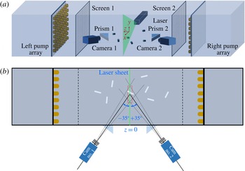
Schematic of experimental set-up: (a) three-dimensional view showing tank, jet arrays, laser sheet, particles, particle-isolation screens, prisms and cameras; (b) top view highlighting the stereoscopic camera arrangement.

Particles whose size is larger than the Kolmogorov scale interact with turbulence in a complex way, typically that which is classified as two-way coupling. In a two-way-coupled interaction, particles translate and rotate by extracting energy from the surrounding flow field, while at the same time altering the flow around them by their motion. Such interaction can alter the spectrum of turbulent kinetic energy (Tanaka & Eaton Reference Tanaka and Eaton2008). The mechanisms behind spectral alteration are still under investigation, partly because it is difficult to separate particles’ effects on turbulence from their effects on an experiment’s turbulence excitation scheme (Lucci, Ferrante & Elghobashi Reference Lucci, Ferrante and Elghobashi2010). Work to date has identified two competing effects in turbulence–particle interaction: vortex shedding in particle wakes increases turbulence intensity, while increased dissipation is caused by particle drag and the disruption of vortex stretching (Burton & Eaton Reference Burton and Eaton2005; Yeo et al. Reference Yeo, Dong, Climent and Maxey2010; Capecelatro & Desjardins Reference Capecelatro and Desjardins2015; Cisse et al. Reference Cisse, Saw, Gilbert, Bodenschatz and Bec2015). By considering both spherical and non-spherical particles, Bellani et al. (Reference Bellani, Byron, Collignon, Meyer and Variano2012) and Zhao, George & van Wachem (Reference Zhao, George and van Wachem2015a ) also showed that the turbulence alteration could vary depending on particle shape.
Particle rotation has been studied previously for sub-Kolmogorov-scale neutrally buoyant spheroids in homogeneous isotropic turbulence (Shin & Koch Reference Shin and Koch2005; Parsa et al. Reference Parsa, Calzavarini, Toschi and Voth2012; Gustavsson, Einarsson & Mehlig Reference Gustavsson, Einarsson and Mehlig2014; Marcus et al. Reference Marcus, Parsa, Kramel, Ni and Voth2014; Parsa & Voth Reference Parsa and Voth2014; Byron et al. Reference Byron, Einarsson, Gustavsson, Voth, Mehlig and Variano2015). These particles experience linear shear flow locally, so that their rotation can be determined by solving Jeffery’s equation along Lagrangian trajectories computed in direct numerical simulations (DNS). Parsa et al. (Reference Parsa, Calzavarini, Toschi and Voth2012) and Marcus et al. (Reference Marcus, Parsa, Kramel, Ni and Voth2014) confirmed this method’s results with laboratory data. Byron et al. (Reference Byron, Einarsson, Gustavsson, Voth, Mehlig and Variano2015) showed that rotation of spheroids about their symmetry axis depends strongly on particle aspect ratio. Specifically, the rotation of rods is dominated by spinning about their symmetry axis, while discs tend to tumble about one of their other two principal axes. This same trend is seen when particles remain small but have inertia by virtue of their mass (Zhao et al. Reference Zhao, Challabotla, Andersson and Variano2015b ). It is not yet known whether the same dynamics holds for particles larger than the Kolmogorov scale, which have inertia by virtue of their size, even when neutrally buoyant. Some evidence can be gathered from Parsa & Voth (Reference Parsa and Voth2014) who performed laboratory measurements of rotating rods with diameters near the Kolmogorov length scale but lengths well into the inertial range. Due to their size, these particles experience a nonlinear velocity gradient in the carrier fluid; the point-particle assumption fails and Jeffery’s equation can no longer predict their dynamics accurately. Other factors that can lead to deviation from Jeffery’s theory include fluid and particle inertia. Results show that long rods align with fluid vorticity (albeit more weakly than short rods do), which suggests that they will continue to emphasize spinning over tumbling. Herein, we continue along this line of inquiry by directly measuring the spinning of large (and therefore inertial) particles. We also consider a different set of shapes than Parsa & Voth (Reference Parsa and Voth2014), namely wider cylinders whose diameter and length have similar magnitude.
2 Experimental set-up and methods
2.1 Turbulence tank
We perform our experiments in the same rectangular glass tank (80 cm
 $\times$
80 cm
 $\times$
356 cm) used by Bellani et al. (Reference Bellani, Byron, Collignon, Meyer and Variano2012), shown in figure 1(a,b). The origin of our coordinate system is located at the tank centre. The
 $x$
-direction is the lateral (horizontal) direction; the
 $y$
-direction is the vertical direction; and the
 $z$
-direction is the axial direction.
The tank is filled with tap water which is filtered to
 $5~\unicode[STIX]{x03BC}\text{m}$
and purified by continuously pumping through an ultraviolet purifier when the experiments are not running. The tank water is stirred to generate turbulence using two panels of axially aligned, randomly actuated synthetic jet arrays (RASJAs) mounted on two solid dividers 165 cm apart. Each RASJA, located symmetrically 82.5 cm from the
 $z=0$
plane (see figure 1), consists of
 $8\times 8$
pumps on an equally spaced Cartesian grid. The pumps are actuated stochastically by a randomizing algorithm that maximizes the shear production of turbulence (Variano & Cowen Reference Variano and Cowen2008; Pérez-Alvarado, Mydlarski & Gaskin Reference Pérez-Alvarado, Mydlarski and Gaskin2016). Two mesh screens are installed on either side of the test region at a distance 45.5 cm away from each array to prevent damage to the large hydrogel particles added to the tank (see § 2.2). At the tank centre, the turbulence is homogeneous and isotropic, and the signature of individual jets is not discernible. The mean flow everywhere within our measurement region is
 ${<}10\,\%$
of the root-mean-square velocities (Bellani & Variano Reference Bellani and Variano2014).
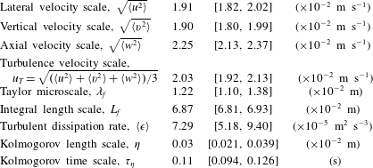
The turbulence properties of the tank are summarized in table 1. The Taylor microscale (
 $\unicode[STIX]{x1D706}_{f}$
) of the flow is estimated by fitting an osculating parabola to the first three points of the longitudinal autocovariance curve (not including the zero-shift point). The dissipation rate (
 $\langle \unicode[STIX]{x1D716}\rangle$
) is calculated in two ways. First,
 $\langle \unicode[STIX]{x1D716}\rangle$
is calculated as a function of
 $\unicode[STIX]{x1D706}_{f}$
assuming isotropy:
 $\langle \unicode[STIX]{x1D716}\rangle =20\unicode[STIX]{x1D708}k^{2}/\unicode[STIX]{x1D706}_{f}^{2}$
. Second,
 $\langle \unicode[STIX]{x1D716}\rangle$
is calculated from the second-order longitudinal structure function using the Kolmogorov scaling and a value of 2.0 as the Kolmogorov constant. The two methods agree, and results from the latter method are given in table 1. The integral length scale (
 $L_{f}$
) is calculated by fitting a Bessel function to the longitudinal autocovariance curve in the inertial subrange (Pope Reference Pope2000; Bellani & Variano Reference Bellani and Variano2014). The uncertainties in the velocities are obtained from bootstrapping (Efron & Tibshirani Reference Efron and Tibshirani1993); the uncertainties in
 $\unicode[STIX]{x1D706}_{f}$
and
 $L_{f}$
are obtained from the ordinary least-square fits; the uncertainties in
 $\langle \unicode[STIX]{x1D716}\rangle$
and Kolmogorov scales are obtained via uncertainty propagation.
Turbulence properties at the location where the particles are measured. The brackets denote 95 % confidence intervals.

2.2 Inertial particles
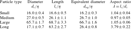
We use four particle types to measure the effect of size and shape: small, medium, large and long. Dimensions of each particle type are provided in table 2. In addition to particle length (
 $l_{c}$
) and diameter (
 $d_{c}$
), we also provide their volume-equivalent spherical diameter,
 $d_{eq}=(d_{c}^{2}l_{c})^{1/3}$
. This length scale will be extensively used in the rest of the manuscript. The particles are made of hydrogel which is 0.4 % Agarose polymer uniformly mixed in deionized water. In order to use particle image velocimetry (PIV) to track the hydrogel particles’ solid-body motion, we dope each particle with tracers. For small, medium and long particles we use
 $13{-}44~\unicode[STIX]{x03BC}\text{m}$
glass spheres (class 4a, size 3200, Cataphote Inc.). For large particles we use commercial glitter (GX-231U ultra-fine crystal glitter, Mark Enterprises). The hydrogel solution is manufactured by allowing a mixture of water, Agarose and tracers to solidify to a rectangular sheet, after which particles are cut out using straight stainless-steel tubes. The hydrogel particles experience slight change in their dimensions due to water desorption under prolonged (
 ${\sim}24$
h) exposure to surrounding water. We accounted for this change during manufacturing by cutting the particles larger than their intended size. All dimensions given herein are steady-state values after water desorption.
The benefit of using hydrogel as the solid phase is twofold. First, since their primary constituent is water (99.6 %), particles are near-neutrally buoyant (specific gravity,
 $SG=1.003\pm 0.001$
), so that the effect of gravity on their overall motion is minimal. Secondly, the hydrogel’s refractive index,
 $RI=1.3329$
is closely matched with that of water, which allows optical methods to obtain a distortion-free velocity field within and outside the particle using PIV. These issues are discussed in further detail in Byron & Variano (Reference Byron and Variano2013).
Dimensions of hydrogel cylinders normalized by Kolmogorov length scale. Uncertainties in
 $d_{c}$
and
 $l_{c}$
are 95 % confidence interval obtained from a t test distribution based on 30 independent samples. Uncertainty in
 $d_{eq}$
(volume-equivalent spherical diameter) is estimated via uncertainty propagation.

2.3 Time scale analysis
The particle dimensions considered in this study are within the inertial subrange of the surrounding turbulence. At this scale (
 $d_{eq}>\unicode[STIX]{x1D702}$
), it is inaccurate to consider the Stokesian relaxation time
 $$\begin{eqnarray}\unicode[STIX]{x1D70F}_{\unicode[STIX]{x1D708}}=\frac{1}{18}\frac{SGd_{p}^{2}}{\unicode[STIX]{x1D708}}\end{eqnarray}$$
as a characteristic time scale of the particle, because it may be moving relative to fluid with significant velocity. Even if the relative velocity is small, the flow far from the particle is not uniform, disrupting the assumptions made in Stokes flow. For a finite Reynolds number particle, the characteristic time scale (
 $\unicode[STIX]{x1D70F}_{p}$
) is related to
 $\unicode[STIX]{x1D70F}_{\unicode[STIX]{x1D708}}$
as (Xu & Bodenschatz Reference Xu and Bodenschatz2008),
 $$\begin{eqnarray}\unicode[STIX]{x1D70F}_{p}=\unicode[STIX]{x1D70F}_{\unicode[STIX]{x1D708}}\frac{24}{Re_{p}C_{D}}.\end{eqnarray}$$
Here,
 $Re_{p}=u_{T}d_{eq}/\unicode[STIX]{x1D708}$
is a Reynolds number based on the turbulence velocity scale (
 $u_{T}$
, defined in table 1) and a particle’s volume-equivalent spherical diameter (
 $d_{eq}$
);
 $C_{D}$
is the drag coefficient of the particle, evaluated at
 $Re=Re_{p}$
.
Specifying
 $C_{D}$
for non-spherical particles at an intermediate Reynolds number (
 $Re_{p}\sim 10^{2}$
) is non-trivial. For the current analysis, we choose to adopt a method comprehensively described in Loth (Reference Loth2008). It follows from a dimensional analysis (see Ganser Reference Ganser1983), wherein the shape variation in the Stokes-drag regime (
 $f_{shape}$
) is combined with shape variation in the Newton-drag regime (
 $C_{shape}$
) to obtain two normalized quantities:
 $$\begin{eqnarray}\displaystyle & \displaystyle Re_{p}^{\ast }=\frac{C_{shape}Re_{p}}{f_{shape}}, & \displaystyle\end{eqnarray}$$
 $$\begin{eqnarray}\displaystyle & \displaystyle C_{D}^{\ast }=\frac{C_{D}}{C_{shape}}. & \displaystyle\end{eqnarray}$$
The creeping-flow shape parameter
 $f_{shape}$
is defined as:
 $$\begin{eqnarray}f_{shape}={\textstyle \frac{1}{3}}\sqrt{A_{surf}^{\ast }}+{\textstyle \frac{2}{3}}\sqrt{A_{proj}^{\ast }},\end{eqnarray}$$
where the area terms are the shape’s surface area and projected area, each normalized by the corresponding area for a volume-equivalent sphere. For a cylindrical particle with aspect ratio
 $\unicode[STIX]{x1D706}$
,
 $$\begin{eqnarray}A_{surf}^{\ast }=\frac{2\unicode[STIX]{x1D706}+1}{(18\unicode[STIX]{x1D706}^{2})^{1/3}}.\end{eqnarray}$$
 $A_{proj}^{\ast }$
depends on the orientation of the particle relative to the flow. Considering all three principal orientations of the particle to be equally likely in turbulence, we obtain a mean
 $\langle A_{proj}^{\ast }\rangle$
for a cylinder as,
 $$\begin{eqnarray}\langle A_{proj}^{\ast }\rangle =\frac{1}{3}(A_{proj,\Vert }^{\ast }+2A_{proj,\bot }^{\ast })=\frac{1}{3}\left(\frac{8\unicode[STIX]{x1D706}}{\unicode[STIX]{x03C0}}+1\right)\left(\frac{3\unicode[STIX]{x1D706}}{2}\right)^{-2/3}.\end{eqnarray}$$
The Newtonian regime shape parameter,
 $C_{shape}$
, is defined as the drag coefficient of the particle normalized by the drag coefficient of a volume-equivalent sphere. It can be approximated by the empirical relations (Loth Reference Loth2008):
 $$\begin{eqnarray}\displaystyle C_{shape} & {\approx} & \displaystyle 1+1.5(A_{surf}^{\ast }-1)^{1/2}+6.7(A_{surf}^{\ast }-1),\quad \unicode[STIX]{x1D706}\leqslant 1\nonumber\\ \displaystyle & {\approx} & \displaystyle 1+0.7(A_{surf}^{\ast }-1)^{1/2}+2.4(A_{surf}^{\ast }-1),\quad \unicode[STIX]{x1D706}>1.\end{eqnarray}$$
In order to estimate the time scale
 $\unicode[STIX]{x1D70F}_{p}$
for our cylinders (cf. (2.2)), we first estimate the two shape parameters
 $f_{shape}$
and
 $C_{shape}$
using (2.5) and (2.8) respectively. We use these parameters and
 $Re_{p}$
to compute
 $Re_{p}^{\ast }$
using (2.3). The normalized drag coefficient (
 $C_{D}^{\ast }$
) then follows from the dimensionless Clift–Gauvin expression given by Leith (Reference Leith1987),
 $$\begin{eqnarray}C_{D}^{\ast }=\frac{24}{Re_{p}^{\ast }}[1+0.15(Re_{p}^{\ast })^{0.687}]+\frac{0.42}{1+{\displaystyle \frac{0.42}{(Re_{p}^{\ast })^{1.16}}}}.\end{eqnarray}$$
Finally, the drag coefficient (
 $C_{D}$
) needed to rescale the particle relaxation time is evaluated from (2.4).
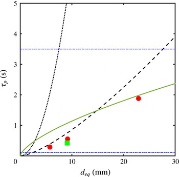
Figure 2 shows the characteristic time scale (
 $\unicode[STIX]{x1D70F}_{p}$
) for the particles used in this study. For all particles,
 $\unicode[STIX]{x1D70F}_{p}$
falls between the large-eddy turnover time of turbulence (
 $L_{f}/(k)^{0.5}=3.5$
s) and the Kolmogorov time scale (
 $\unicode[STIX]{x1D70F}_{\unicode[STIX]{x1D702}}=0.11$
s). Thus, the particles are within the inertial subrange of turbulence when considering both time and length scales. A turnover time (
 $\unicode[STIX]{x1D70F}_{d}$
) corresponding to turbulent motions of size scale
 $d_{eq}$
can be defined as:
 $$\begin{eqnarray}\unicode[STIX]{x1D70F}_{d}\sim d_{eq}^{(2/3)}\langle \unicode[STIX]{x1D716}\rangle ^{(-1/3)}.\end{eqnarray}$$
Figure 2 shows that
 $\unicode[STIX]{x1D70F}_{p}<\unicode[STIX]{x1D70F}_{d}$
for each particle size, and therefore suggests that particles considered in this study have a characteristic time scale fast enough to respond to motions of their size. Computing Stokes number as
 $\unicode[STIX]{x1D70F}_{p}/\unicode[STIX]{x1D70F}_{d}$
, we find the following values for the four particle types: 0.36 for small, 0.51 for medium 0.4 for long and 0.95 for large.
Relationship between time scale and length scale for different shapes and assumptions. Points represent the four particles considered herein: small, medium and large cylinders of aspect ratio 1 (●) and long cylinders of aspect ratio 4 (▪) computed via (2.2)–(2.9). Horizontal lines (–
 $\cdot$
–
 $\cdot$
–) indicate the Kolmogorov microscale and large-eddy turnover time in our laboratory flow. The space–time relationship for motions in the inertial subrange according to the Richardson–Kolmogorov model (see (2.10)) is given by the solid line (——). The dotted line (
 $\cdots \cdots$
) gives the time scale for spheres in creeping flow according to Stokes’ formula (see (2.1)) and the dashed line (– – – –) gives the time scale using the Clift–Gauvin relationship for spheres.

2.4 Two-phase stereoscopic PIV for particles and fluid
We perform stereoscopic PIV to obtain two-dimensional three-component (2D3C) velocity fields simultaneously in both fluid and particle phases. The fluid phase is seeded with
 $13~\unicode[STIX]{x03BC}\text{m}$
silver-coated hollow glass spheres (SH400S20, Potters Industries). The measurement plane (
 $z=0$
) is illuminated by a laser sheet (1 mm thick; Quantel/Big Sky Lasers, 532 nm) that bisects the tank. The laser-illuminated region of interest is imaged by two charge-coupled device (CCD) cameras (Imager PRO-X, 1600 pixels
 $\times$
1200 pixels), each camera being frame straddled to synchronize with the dual pulse of the laser. The image pairs are collected at a frame rate of 14.0 Hz, with a pulse separation of 6 ms. The two cameras are stereoscopically aligned on either side of the laser sheet such that the camera line of sight is
 $\pm 55^{\circ }$
off-normal from the measurement plane. In order to minimize optical distortion due to this angle, each camera views the measurement plane through a custom-made
 $35^{\circ }$
water-filled acrylic prism. The arrangement of our PIV system is schematically shown in figure 1(b). A Nikkor 85 mm lens, equipped with a circular polarizer, is mounted on each camera using a Scheimpflug adapter. Each polarizer is independently adjusted to obtain sufficient contrast to resolve the tracers in the fluid and inside the particles. Care is needed in the latter case because the hydrogel scatters a small amount of light, giving particles a moderately bright appearance which competes with the light scattering from the embedded tracers.
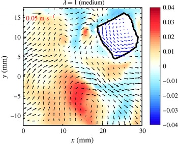
Sample velocity field in the particle phase (blue arrows) and fluid phase (black arrows) for a
 $\unicode[STIX]{x1D706}=1$
particle (medium type). The red and blue contours show the out-of-plane velocity component (
 $u_{z}$
; (
 $\text{cm}~\text{s}^{-1}$
)) in the fluid phase, and are measured but not shown in the particle phase. The example vector in the upper left corresponds to
 $0.05~\text{m}~\text{s}^{-1}$
for the fluid phase. The vectors within the particle phase are magnified by a factor of 3. Every other vector is omitted in the fluid phase for clarity.

The velocity field inside and outside the particle is computed using DaVis 8.2 software (LaVision GmbH). Within the hydrogel particle, tracers are locked in place, and thus the in-particle velocity field shows solid-body motion. The in-particle velocity field is computed as follows. First, the particle phase is identified by intensity thresholding, using the fact that particles appear brighter than the fluid but less bright than tracers. The fluid phase is masked and multipass stereoscopic cross-correlation is applied to the tracers within the particle. The cross-correlation is applied with an initial interrogation window of 128 pixels
 $\times$
128 pixels and final window of 64 pixels
 $\times$
64 pixels with 50 % overlap. A weighting function is applied to the image interrogation windows to improve accuracy (Raffel et al.
Reference Raffel, Willert, Wereley and Kompenhans2007). The weighting function used for the 64
 $\times$
64 window is a symmetric two-dimensional Gaussian with
 $\unicode[STIX]{x1D70E}=31$
pixels
 $=$
0.87 mm, whose area within
 $2\unicode[STIX]{x1D70E}=9.51~\text{mm}^{2}$
. The spacing between vectors is 0.9 mm for the final-pass calculations. This grid spacing is
 $0.2d_{eq}$
for the smallest particle, and therefore sufficiently small to resolve the velocity field inside each particle. Figure 3 shows a representative sample demonstrating the solid-body rotation of a medium particle as well as the flow field in the carrier fluid. Velocity fields in the fluid phase are computed with a similar method as described above (for particle-phase velocities). The multipass cross-correlation interrogation window size for the fluid phase progresses from 96 pixels
 $\times$
96 pixels to 32 pixels
 $\times$
32 pixels in the final pass. The two-dimensional Gaussian weighting function has
 $\unicode[STIX]{x1D70E}=15$
pixels, so that the area within
 $2\unicode[STIX]{x1D70E}=2.23~\text{mm}^{2}$
. The interrogation areas have 50 % overlap, so that the spacing between fluid-phase velocity vectors is 0.45 mm. This spacing is finer than that used for the particle-phase velocity because tracers in the fluid are imaged more clearly than tracers embedded within particles. The velocity statistics are similar in both phases, though there can be some significant instantaneous differences due to particle slip, discussed by Byron (Reference Byron2015).
2.5 Rotation and orientation
Particle angular velocity (
 $\unicode[STIX]{x1D734}$
) is computed from the stereoscopic PIV velocity field within the solid phase using the equation of solid-body rotation:
 $$\begin{eqnarray}\boldsymbol{u}_{m}=\boldsymbol{u}_{n}+\unicode[STIX]{x1D734}\times (\boldsymbol{r}_{m}-\boldsymbol{r}_{n}),\end{eqnarray}$$
where subscripts
 $m$
and
 $n$
refer to any two locations within the solid object, and
 $\unicode[STIX]{x1D734}\;(=\unicode[STIX]{x1D6FA}_{i})$
is defined relative to the particle centre of mass. Since all our experimental data are coplanar with the
 $z=0$
plane, the system of (2.11) is over-determined in
 $\unicode[STIX]{x1D6FA}_{z}$
and under-determined in
 $\unicode[STIX]{x1D6FA}_{x}$
and
 $\unicode[STIX]{x1D6FA}_{y}$
, which we resolve by considering three vectors instead of two (Bellani et al.
Reference Bellani, Byron, Collignon, Meyer and Variano2012).
For each particle type, a large number of particles are measured, giving
 ${\sim}$
1000 independent samples. For each sample, we solve (2.11) with all possible triplets of vectors within the particle and then take the median as the measured
 $\unicode[STIX]{x1D6FA}_{i}$
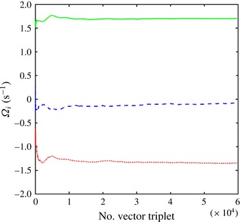
. During this computation, we ensure that (i) the particle measurement section contains at least 10 vectors and (ii)
 $\unicode[STIX]{x1D6FA}_{i}$
converges such that the change in
 $\unicode[STIX]{x1D6FA}_{i}$
that occurs when removing one of the triplets is less than 0.1 % of
 $(\unicode[STIX]{x1D6FA}_{i}\unicode[STIX]{x1D6FA}_{i})^{1/2}$
(see figure 4).
Particle angular velocity (
 $\unicode[STIX]{x1D6FA}_{i}$
) with respect to the number of vector triplets used to calculate
 $\unicode[STIX]{x1D6FA}_{x}$
(
 $\cdots \cdots$
),
 $\unicode[STIX]{x1D6FA}_{y}$
(– – –),
 $\unicode[STIX]{x1D6FA}_{z}$
(——) for the sample flow field shown in figure 3.

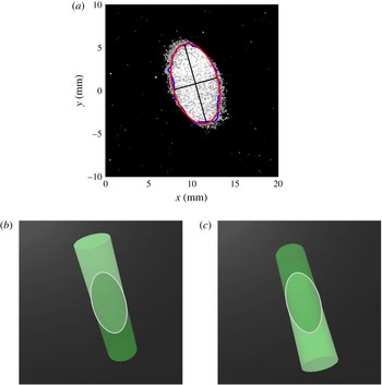
(a) Sample orthonormal view of a particle reconstructed in DaVis 8.2 from two raw stereoscopic images. The blue line indicates the boundary of the particle’s illuminated section and the red line indicates the fitted ellipse. (b,c) Orthonormal views recreated in Maya 2014 (Autodesk) using
 $\unicode[STIX]{x1D6FD}_{1}$
(b) and
 $\unicode[STIX]{x1D6FD}_{2}$
(c), showing that both values give the same elliptical secant plane.

Orientation is obtained for long particles (
 $\unicode[STIX]{x1D706}=4$
) only. The method uses the particle cross-section (i.e. the secant plane) intersected by the laser sheet. The secant plane of a particle is an ellipse unless the laser sheet intersects the particle end caps. Here, we consider only the full elliptical cross-sections, restricting our analysis to particles in which the laser sheet does not intersect the end caps. This does not introduce a sampling bias, because the fluid and particle dynamics are isotropic. A total of 500 particles pass the restriction and are discussed below.
We analyse the elliptical secant plane from the perspective of a reconstructed orthonormal view (i.e. what a camera perpendicular to the laser sheet would see) computed in DaVis 8.2. Figure 5(a) shows a sample orthonormal reconstruction. This image is processed separately in MATLAB through the following operations to obtain the ellipse highlighted in figure 5(a). First, a threshold filter is applied to the image to identify the area of interest. Next, the image is converted to the binary format, and a median filter is applied to remove the high-intensity tracer particles within the surrounding fluid phase. A morphological closing is then applied to fill ‘holes’ or ‘craters’ in the particle section. Finally, an ellipse is fitted along the cross-sectional boundary of the particle using the method of least squares. The least-square root-mean-square error for a fit is typically 5 pixels (0.14 mm). The fit results are insensitive to the image intensity thresholding, within a reasonable range of thresholds.
The secant plane ellipse is analysed to obtain two geometric features: the tilt angle (
 $\unicode[STIX]{x1D6FC}$
,
 $0<\unicode[STIX]{x1D6FC}<180^{\circ }$
) is the angle between the minor axis and the horizontal; the secant aspect ratio
 $\unicode[STIX]{x1D706}_{s}$
is the minor-to-major axis aspect ratio. Note that the minor axis length is equal to diameter of the particle. The aspect ratio
 $\unicode[STIX]{x1D706}_{s}$
is related to particle inclination angle
 $\unicode[STIX]{x1D6FD}$
, made by the laser sheet with the plane normal to the particle’s symmetry axis, as
 $\unicode[STIX]{x1D6FD}=\text{cos}^{-1}\unicode[STIX]{x1D706}_{s}$
.
The values of
 $\unicode[STIX]{x1D6FC}$
and
 $\unicode[STIX]{x1D6FD}$
determine the orientation of the particle, to within a single ambiguity. That is, there are two supplementary inclination angles,
 $\unicode[STIX]{x1D6FD}_{1}$
,
 $0<\unicode[STIX]{x1D6FD}_{1}<90^{\circ }$
and
 $\unicode[STIX]{x1D6FD}_{2}$
,
 $90<\unicode[STIX]{x1D6FD}_{2}<180^{\circ }$
(
 $\unicode[STIX]{x1D6FD}_{1}+\unicode[STIX]{x1D6FD}_{2}=180^{\circ }$
), that will result in the same elliptical cross-section where the particle and the light sheet intersect. This ambiguity is demonstrated in figure 5(b,c) using two orthonormal views recreated in Maya 2014 (Autodesk). We resolve the ambiguity in
 $\unicode[STIX]{x1D6FD}$
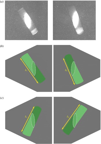
by visually inspecting each of the 500 raw stereoscopic image pairs considered herein. In a stereoscopic arrangement the two cameras view the object plane from two independent angles, thus each camera records a different projection of the particle. The total length of the projected particle will be different in the two images. We can determine which of the two candidate angles (
 $\unicode[STIX]{x1D6FD}_{1}$
and
 $\unicode[STIX]{x1D6FD}_{2}$
) is accurate by comparing the projected particle lengths in cameras 1 and 2 (
 $L_{1}$
and
 $L_{2}$
) via the following rules:
 $$\begin{eqnarray}\left.\begin{array}{@{}c@{}}L_{1}>L_{2}\Rightarrow \unicode[STIX]{x1D6FD}=\unicode[STIX]{x1D6FD}_{1},\\ L_{1}<L_{2}\Rightarrow \unicode[STIX]{x1D6FD}=\unicode[STIX]{x1D6FD}_{2},\\ L_{1}=L_{2}\Rightarrow \unicode[STIX]{x1D6FD}_{1}=\unicode[STIX]{x1D6FD}_{2}=\unicode[STIX]{x03C0}/2.\end{array}\right\}\end{eqnarray}$$
This rule works for approximately 65 % of the measured particles. When the rule is ambiguous because
 $L_{1}\approx L_{2}$
, we resolve the ambiguity by comparing the stereoscopic image pair to an optical model of particle appearances created in Maya 2014. In the optical model, particle orientation is specified via an extrinsic rotation of the order
 $x{-}y{-}z$
(one of the Tait–Bryan options) by amounts
 $\unicode[STIX]{x1D6FD}$
, 0 and
 $\unicode[STIX]{x1D6FC}$
respectively, starting from an initial alignment of the symmetry axis in positive
 $y$
. Virtual cameras in Maya 2014 provide synthetic stereoscopic images, which we then compare to the images collected in the laboratory. For one of the candidate
 $\unicode[STIX]{x1D6FD}$
values, the real and virtual images match very well, and for the other they match poorly. This allows us to resolve the orientational ambiguity for all samples for which (2.12) is insufficient. One representative case comparing a stereoscopic image pair with its
 $\unicode[STIX]{x1D6FD}_{1}$
and
 $\unicode[STIX]{x1D6FD}_{2}$
is shown in figure 6.
Stereoscopic images (i.e. not orthonormal to the laser sheet) (a) obtained from cameras 1 and 2 with intensity scale set to emphasize the secant plane, (b) recreated in Maya 2014 using
 $\unicode[STIX]{x1D6FD}_{1}$
(
 $L_{1}>L_{2}$
); (c) recreated in Maya 2014 using
 $\unicode[STIX]{x1D6FD}_{2}$
(
 $L_{1}<L_{2}$
). The secant planes in (b,c) are shown in dashed lines for visual guidance. Clearly (a,b) are a better match than (a,c).

PDF of the three components of angular velocity (
 $\unicode[STIX]{x1D6FA}_{x}$
: ●,
 $\unicode[STIX]{x1D6FA}_{y}$
: ▪,
 $\unicode[STIX]{x1D6FA}_{z}$
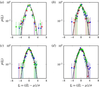
: ♦) for (a) small, (b) medium, (c) large and (d) long particles. The error bars represent 95 % confidence level obtained via bootstrapping. The solid curve is a normal distribution.

From
 $\unicode[STIX]{x1D6FC}$
and
 $\unicode[STIX]{x1D6FD}$
, which completely describe the particle orientation, we compute the direction vector
 $n_{i}$
of the particle symmetry axis as follows:
 $$\begin{eqnarray}\left.\begin{array}{@{}c@{}}n_{1}=\sin \unicode[STIX]{x1D6FC}\cdot \cos \unicode[STIX]{x1D6FD},\\ n_{2}=-\text{cos}\,\unicode[STIX]{x1D6FC}\cdot \cos \unicode[STIX]{x1D6FD},\\ n_{3}=-\text{sin}\,\unicode[STIX]{x1D6FD}.\end{array}\right\}\end{eqnarray}$$
We decompose the angular velocity
 $\unicode[STIX]{x1D6FA}_{i}$
of each particle based on its orientation
 $n_{i}$
. The rotation rate which is parallel to the particle symmetry axis is referred to as its spinning rate,
 $\unicode[STIX]{x1D6FA}_{\Vert }=n_{i}\unicode[STIX]{x1D6FA}_{i}$
. The tumbling rate,
 $\unicode[STIX]{x1D6FA}_{\bot }$
is the sum of rotation rates along the two equatorial axes of the particle, such that
 $|\unicode[STIX]{x1D6FA}_{\bot }|^{2}=|\unicode[STIX]{x1D6FA}|^{2}-|\unicode[STIX]{x1D6FA}_{\Vert }|^{2}$
.
3 Results and discussion
3.1 Particle angular velocity
We begin our investigation with the probability distribution of angular velocity (
 $\unicode[STIX]{x1D6FA}_{i}$
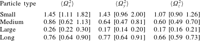
) for each of the four particle types. Figure 7 shows the normalized probability density function (PDF) of each component of particle angular velocity. Table 3 lists the second moment of these distributions with their respective 95 % confidence levels obtained via bootstrapping 1000 replicates. There were inherent practical limitations to the rate of data collection. For example, due to our choice to keep the particle volume fraction low and collect images of high resolution and large magnification, the data collection rate was limited to
 $O(10)$
particle images per hour. Thus our overall experiment was restricted to a small number of samples, specifically (500–1000 independent samples for each particle type). Given this limitation, complete convergence of statistics was not always possible, especially for the higher-order moments of
 $\unicode[STIX]{x1D6FA}_{i}$
. The confidence intervals calculated via bootstrap accurately indicate the wide spread of possible values that the statistical moments could take.
Variance of particle angular velocity components (
 $\text{s}^{-2}$
) for each of the cylindrical particle types considered in this study. The bracketed quantities represent 95 % confidence level obtained via bootstrapping.

All three components of
 $\unicode[STIX]{x1D6FA}_{i}$
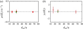
follow a symmetric distribution within the uncertainty of the measurements (see figure 7), suggesting that the third moment is zero. The first and third moments of the measured
 $\unicode[STIX]{x1D6FA}_{z}$
values are shown in figure 8, and confirm isotropy with respect to the laboratory frame, because each distribution is mean free and skewness free. Isotropy is also evident in the variance data (table 3). The variance of
 $\unicode[STIX]{x1D6FA}_{y}$
(rotation about the direction in which gravity points) does not show any measurable difference from that of the other two components, meaning that gravity does not disrupt isotropy. Given the observed isotropy, we choose
 $\unicode[STIX]{x1D6FA}_{z}$
as a representative component of angular velocity to examine further. Measurements of
 $\unicode[STIX]{x1D6FA}_{z}$
have less noise than the other two components because the laser sheet is in the
 $z$
-direction.
(a) Mean and (b) skewness of the axial component of angular velocity (
 $\unicode[STIX]{x1D6FA}_{z}$
) for cylinders with aspect ratio
 $\unicode[STIX]{x1D706}=1$
(●) and
 $\unicode[STIX]{x1D706}=4$
(▪). The abscissa shows their size, as the diameter of a sphere with equivalent volume. The error bars represent 95 % confidence level obtained via bootstrapping.

We next consider the magnitude of angular velocity variance (
 $\langle \unicode[STIX]{x1D6FA}_{i}\unicode[STIX]{x1D6FA}_{i}\rangle$
) and how it scales with particle size. Based on a dimensional argument, Parsa & Voth (Reference Parsa and Voth2014) proposed that the mean square tumbling rate of long fibres with length in the inertial range of turbulence scales as
 $\langle {\dot{n}}_{i}{\dot{n}}_{i}\rangle \sim \ell ^{-4/3}$
, where
 $n_{i}$
is the orientation vector and
 $\ell$
is the length of a fibre. Their experimental results did not exactly match the prediction, and showed a slope steeper than
 $-4/3$
in the inertial regime (
 $20\unicode[STIX]{x1D702}<\ell <50\unicode[STIX]{x1D702}$
). Our results are not directly comparable with theirs because our particles have both length and diameter larger than
 $\unicode[STIX]{x1D702}$
, and because we measure total angular velocity while they measured only the tumbling rate. That is, since their estimation of rotation rate was based on rod orientation, it did not include the component of rotation along the particle axis (i.e. ‘spinning’).
To predict the variance of particle angular velocity,
 $\langle \unicode[STIX]{x1D6FA}_{i}\unicode[STIX]{x1D6FA}_{i}\rangle$
, we follow a similar dimensional argument as Parsa & Voth (Reference Parsa and Voth2014), but propose to use a different length scale. Instead of the longest particle dimension, we use the volume-equivalent spherical diameter (
 $d_{eq}$
) of the particle, which is also the geometric mean of all three principal dimensions. From dimensional analysis, the mean particle enstrophy
 $\langle \unicode[STIX]{x1D6FA}_{i}\unicode[STIX]{x1D6FA}_{i}\rangle$
scales as
 $1/\unicode[STIX]{x1D70F}_{d}^{2}$
. This argument is supported by the values of
 $\langle \unicode[STIX]{x1D6FA}_{i}\unicode[STIX]{x1D6FA}_{i}\rangle \unicode[STIX]{x1D70F}_{d}^{2}$
, which for the small, medium, large and long particles are 2.312, 2.2, 2.277 and 2.376 respectively. Choosing the time scale (
 $\unicode[STIX]{x1D70F}_{d}$
) introduced in § 2.3,
 $\unicode[STIX]{x1D70F}_{d}\sim d_{eq}^{(2/3)}\langle \unicode[STIX]{x1D716}\rangle ^{(-1/3)}$
and invoking the Kolmogorov scales, we obtain a simplified scaling relationship:
 $$\begin{eqnarray}\langle \unicode[STIX]{x1D6FA}_{i}\unicode[STIX]{x1D6FA}_{i}\rangle \unicode[STIX]{x1D70F}_{\unicode[STIX]{x1D702}}^{2}\sim (d_{eq}/\unicode[STIX]{x1D702})^{-4/3}.\end{eqnarray}$$
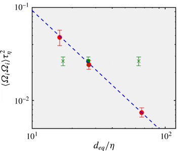
This scaling argument is tested in figure 9, which shows that data for all particle shapes agree very well with the
 ${\sim}(d_{eq}/\unicode[STIX]{x1D702})^{-4/3}$
scaling. For the long (
 $\unicode[STIX]{x1D706}=4$
) particle, neither of the other possible length scales (width or length) cause the data to collapse onto the power-law curve; this reinforces the relevance of scaling based on
 $d_{eq}$
. A least-square fit to the data for small, medium, large and long particles gives the following parameters: enstrophy
 $\langle \unicode[STIX]{x1D6FA}_{i}\unicode[STIX]{x1D6FA}_{i}\rangle \unicode[STIX]{x1D70F}_{\unicode[STIX]{x1D702}}^{2}=1.88(d_{eq}/\unicode[STIX]{x1D702})^{-1.32}$
. If the power-law exponent is fixed at
 $-4/3$
, the constant of proportionality is 1.98
 $\pm$
0.07.
Normalized particle enstrophy (i.e. variance of rotation rate) as a function of particle size (i.e. normalized volume-equivalent spherical diameter). Aspect ratios
 $\unicode[STIX]{x1D706}=1$
(●) and
 $\unicode[STIX]{x1D706}=4$
(▪). The dashed line (– – – –) shows the power-law fit. The cross symbols (
 $\times$
) show the same data point as the green square replotted with respect to the cylinder’s length and width instead of its volume-equivalent spherical diameter. The error bars represent 95 % confidence level obtained via bootstrapping.

Distributions of
 $\unicode[STIX]{x1D6FA}_{i}$
also show an interesting pattern with respect to higher-order moments. For the medium, large and long particles with
 $d_{eq}>27\unicode[STIX]{x1D702}$
, distributions of
 $\unicode[STIX]{x1D6FA}_{i}$
closely follow a standard normal curve with limited evidence of high angular velocity events (see figure 7
b–d). On the other hand, we observe strong evidence of high angular velocity events (
 $|\unicode[STIX]{x1D6FA}_{i}|>3\unicode[STIX]{x1D70E}$
) for the small (
 $d_{eq}=16\unicode[STIX]{x1D702}$
) particles (see figure 7
a). The nearly normal distributions of
 $\unicode[STIX]{x1D6FA}_{i}$
for particles with
 $d_{eq}>27\unicode[STIX]{x1D702}$
suggest that they do not respond, in any distinct way, to the intermittency of the surrounding turbulence. Such ‘internal intermittency’ typically appears as super-Gaussian distributions (i.e. leptokurtic, or kurtosis
 ${>}$
3) of velocity differences, and is attributed to long and skinny vortex lines in the flow. Further insight follows from variance and kurtosis of
 $\unicode[STIX]{x1D6FA}_{i}$
distributions, which we discuss in § 3.2.
3.2 Inheritance of fluid vorticity
Following the kinematic significance of
 $d_{eq}$
, we can revisit the proposal by Bellani et al. (Reference Bellani, Byron, Collignon, Meyer and Variano2012) that finite-sized particles rotate by inheriting the fluid vorticity filtered through some spatial scale. We hypothesize that the proper filtering scale is
 $d_{eq}$
. Describing particle rotation as a spatial filter is at best a first-order approximation, because it is based entirely upon the instantaneous flow field, and thus does not include the temporal filtering caused by particle inertia. However, the results may be useful to qualitatively understand the effect of surrounding flow on particle rotation. We test this hypothesis as follows.
We compute the out-of-plane fluid vorticity (
 $\unicode[STIX]{x1D714}_{z}$
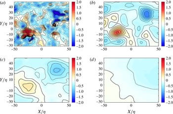
) on a square grid of resolution 0.45 mm using the second-order central difference scheme implemented in DaVis 8.2 (LaVision GmbH). The fluid vorticity is computed only on those fields where no particle is present in the measurement region. We choose a finer resolution for this computation than that for the in-particle velocity computation so that our grid spacing is close to the Kolmogorov scale (
 $\unicode[STIX]{x1D702}=0.3$
mm). Figure 10(a) shows an example vorticity (
 $\unicode[STIX]{x1D714}_{z}$
) field chosen from a database of 1500 independent samples. For our analysis, we consider only those fields for which no particles appear in the measurement region. This exclusion avoids contamination of local velocity gradients by particle boundary layers or wakes.
(a) Example measurement of one component of fluid vorticity (
 $\unicode[STIX]{x1D714}_{z}$
,
 $\text{s}^{-1}$
). (b–d) Same vorticity field filtered through a two-dimensional Gaussian filter of spatial scale
 $16\unicode[STIX]{x1D702}$
,
 $27\unicode[STIX]{x1D702}$
and
 $67\unicode[STIX]{x1D702}$
respectively.

To obtain the filtered vorticity
 ${\mathcal{F}}(\unicode[STIX]{x1D714}_{z})$
, we apply a two-dimensional circular Gaussian filter to the raw vorticity (
 $\unicode[STIX]{x1D714}_{z}$
) fields. We set the size of the Gaussian window equal to
 $d_{eq}$
, such that its standard deviation
 $\unicode[STIX]{x1D70E}=1/3d_{eq}$
. We apply a two-dimensional Gaussian low-pass filter to the vorticity field, with filter window size equal to
 $d_{eq}$
and filter width
 $\unicode[STIX]{x1D70E}_{f}=d_{eq}/3$
. This filter attenuates by 99 % all motions with a length scale less than
 $0.7d_{eq}$
. It attenuates by 50 % motions with length scale of
 $1.8d_{eq}$
and it attenuates motions larger than
 $15d_{eq}$
by less than 1 %. To demonstrate the effect of filter size on the vorticity field, we show in figure 10(b–d) the same vorticity field chosen in figure 10(a) filtered through window sizes of
 $16\unicode[STIX]{x1D702}$
,
 $27\unicode[STIX]{x1D702}$
and
 $67\unicode[STIX]{x1D702}$
respectively.
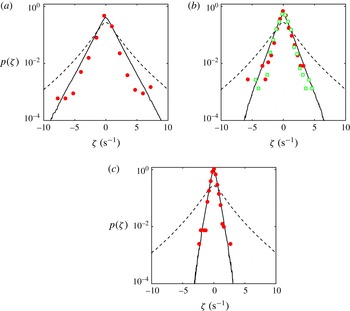
The results in figure 11 compare the distributions of particle angular velocity with those of fluid angular velocity (
 $\unicode[STIX]{x1D701}=\unicode[STIX]{x1D714}_{z}/2$
) and filtered fluid angular velocity (
 ${\mathcal{F}}(\unicode[STIX]{x1D701})$
). The results show that the filtered fluid angular velocity
 ${\mathcal{F}}(\unicode[STIX]{x1D701})$
captures the general trend in the distribution of
 $\unicode[STIX]{x1D6FA}_{z}$
much better than the unaltered
 $\unicode[STIX]{x1D701}$
field. For small (
 $d_{eq}\sim 16\unicode[STIX]{x1D702}$
) particles, the shape of the distribution is clearly different between
 $\unicode[STIX]{x1D6FA}_{z}$
and
 ${\mathcal{F}}(\unicode[STIX]{x1D701})$
, especially at larger rotation rates. The agreement between
 ${\mathcal{F}}(\unicode[STIX]{x1D701})$
and
 $\unicode[STIX]{x1D6FA}_{z}$
becomes better with increasing particle size, so that the distribution of
 $\unicode[STIX]{x1D6FA}_{z}$
collapses on that of
 ${\mathcal{F}}(\unicode[STIX]{x1D701})$
for the largest particle size (
 $d_{eq}\sim 67\unicode[STIX]{x1D702}$
).
PDF of particle angular velocity,
 $\unicode[STIX]{x1D6FA}_{z}$
(●: small, medium and large; ▫: long particles), fluid angular velocity,
 $\unicode[STIX]{x1D714}_{z}$
(– – – –) and fluid angular velocity filtered at particle size
 $d_{eq}$
(——). (a) Small particles; (b) medium and long particles; (c) large particles.

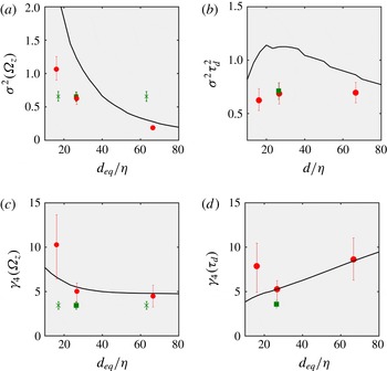
The variance (
 $\unicode[STIX]{x1D70E}^{2}$
) and kurtosis (
 $\unicode[STIX]{x1D6FE}_{4}$
) of
 $\unicode[STIX]{x1D6FA}_{z}$
and
 ${\mathcal{F}}(\unicode[STIX]{x1D701})$
are shown in figure 12. Both quantities decrease with particle size, showing how particles filter out the small-scale motions which are responsible for the majority of vorticity and super-Gaussian behaviour. The high kurtosis (
 $\unicode[STIX]{x1D6FE}_{4}=10.27$
) of
 $\unicode[STIX]{x1D6FA}_{z}$
for the small particles does show a super-Gaussian distribution similar to the unaltered fluid rotation (
 $\unicode[STIX]{x1D6FE}_{4}=14.05$
). The kurtoses for the other three particle types are close to 3 and similar to that of a Gaussian distribution. Comparing the long particles with the medium particles, results show that the latter have greater kurtosis. This is surprising, in that one would expect the long particles to more effectively sample fluid vortices by aligning with them. Figure 12(b,d) show this same behaviour; the normalization highlights the enhanced kurtosis of small particles relative to filtered vorticity and the lower kurtosis of long particles relative to filtered vorticity.
(a) Variance (
 $\unicode[STIX]{x1D70E}^{2}$
), (b) normalized variance (
 $\unicode[STIX]{x1D70E}^{2}\unicode[STIX]{x1D70F}_{d}^{2}$
), (c) kurtosis (
 $\unicode[STIX]{x1D6FE}_{4}$
) (d) normalized kurtosis (
 $\unicode[STIX]{x1D6FE}_{4}\unicode[STIX]{x1D70F}_{d}$
) of the axial component of angular velocity (
 $\unicode[STIX]{x1D6FA}_{z}$
) for cylinders with aspect ratio
 $\unicode[STIX]{x1D706}=1$
(●) and
 $\unicode[STIX]{x1D706}=4$
(▪) and spatially filtered fluid (——). The error bars represent 95 % confidence level obtained via bootstrapping. The cross symbols (
 $\times$
) in (a,d) show the same data points as the green squares replotted with respect to the cylinder’s length and width instead of its volume-equivalent spherical diameter.

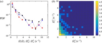
(a) PDF of total enstrophy (♦) and its decomposition into spin (
 ${\unicode[STIX]{x1D6FA}_{\Vert }}^{2}$
: ●) and tumble (
 ${\unicode[STIX]{x1D6FA}_{\bot }}^{2}$
: ▪) components and (b) two-dimensional histogram of
 ${\unicode[STIX]{x1D6FA}_{\Vert }}^{2}$
and
 ${\unicode[STIX]{x1D6FA}_{\bot }}^{2}$
for anisotropic large particle with aspect ratio
 $\unicode[STIX]{x1D706}=4$
(
 $d_{eq}=27\unicode[STIX]{x1D702}$
). The colour bars in (b) show the logarithmic frequency of the two-dimensional histogram.

3.3 Angular velocity decomposition
The angular velocity (
 $\unicode[STIX]{x1D6FA}_{i}$
) of
 $\unicode[STIX]{x1D706}=4$
particles is decomposed into spin (
 $\unicode[STIX]{x1D6FA}_{\Vert }$
) and tumble (
 $\unicode[STIX]{x1D6FA}_{\bot }$
) components following the method discussed in § 2.5. The results are shown in figure 13, with probability density functions of the particle enstrophy and its decomposition into spin enstrophy (
 $\unicode[STIX]{x1D6FA}_{\Vert }^{2}$
) and tumble enstrophy (
 $\unicode[STIX]{x1D6FA}_{\bot }^{2}$
) in figure 13(a). The PDF of each component is similar to the PDF of the total. The ratio between the two components is nearly constant, regardless of the latter’s value. The correlation between spinning enstrophy and tumbling enstrophy is 0.37, meaning that the correlation between the magnitude of
 $|\unicode[STIX]{x1D6FA}_{\Vert }|$
and
 $|\unicode[STIX]{x1D6FA}_{\bot }|$
is 0.61. The two-dimensional histogram of the same data is shown in figure 13(b), demonstrating the cross-correlation between instantaneous values of spin enstrophy (
 ${\unicode[STIX]{x1D6FA}_{\Vert }}^{2}$
) and tumble enstrophy (
 ${\unicode[STIX]{x1D6FA}_{\bot }}^{2}$
). It follows from figure 13(b) that events of high spinning are accompanied by low tumbling and vice versa. In other words, spin and tumble are anti-correlated; when a particle has large angular velocity, that angular velocity manifests almost entirely either as spinning or tumbling motion, not as both.
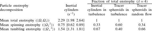
The PDFs in figure 13 have first moments that are listed in table 4. This shows that, for long cylinders, spinning represents close to one-third of the enstrophy, while tumbling represents the other two-thirds. This is strikingly different from the trend seen for infinitesimal particles, which show a dominance of spinning for long spheroids (Parsa et al. Reference Parsa, Calzavarini, Toschi and Voth2012; Byron et al. Reference Byron, Einarsson, Gustavsson, Voth, Mehlig and Variano2015). Results for such ‘tracer rods’ are shown in table 4 for comparison. We calculate these by solving Jeffery’s equations for tracer spheroids in a direct numerical simulation of homogeneous isotropic turbulence, made public in the Johns Hopkins University turbulence database (Li et al. Reference Li, Perlman, Wan, Yang, Meneveau, Burns, Chen, Szalay and Eyink2008; Yu et al. Reference Yu, Kanov, Perlman, Graham, Frederix, Burns, Szalay, Eyink and Meneveau2012), exactly as in Byron et al. (Reference Byron, Einarsson, Gustavsson, Voth, Mehlig and Variano2015) and similar to Parsa et al. (Reference Parsa, Calzavarini, Toschi and Voth2012). We also include in table 4 the results from an analytic treatment of ellipsoid motion in a random flow, extracted from Byron et al. (Reference Byron, Einarsson, Gustavsson, Voth, Mehlig and Variano2015). This random flow shares many of the same statistics as turbulence, but does not have features such as coherent structures and vortex stretching (Gustavsson et al. Reference Gustavsson, Einarsson and Mehlig2014).
Particle enstrophy decomposed into components parallel and orthogonal to the particle’s symmetry axis for long cylinders (
 $\unicode[STIX]{x1D706}=4$
). The bracketed quantities represent 95 % confidence level obtained via bootstrapping. The fourth column is obtained by solving Jeffery’s equation in DNS. The fifth column is obtained by interpolating data from figure 4 in Byron et al. (Reference Byron, Einarsson, Gustavsson, Voth, Mehlig and Variano2015).

Comparison between the three cases in table 4 suggests that enhanced spinning is seen for tracer particles, but not for the large particles measured herein. Spinning occurs about only one principle axis, and tumbling occurs about two axes, so that the result in table 4 suggests equipartition. We emphasize, however, that the result shows only equipartition of enstrophy, not energy. The mean rotational kinetic energy
 $\langle \unicode[STIX]{x1D6FA}_{i}I_{(i,j)}\unicode[STIX]{x1D6FA}_{j}\rangle$
of a particle is dependent on the moment of inertia
 $I_{(i,j)}$
. For cylinders with
 $\unicode[STIX]{x1D706}>1$
,
 $I_{\Vert }\neq I_{\bot }$
, and thus we conclude that the rotational kinetic energy is not equally distributed along the three principal axes. In table 5, we show the partitioning of particle enstrophy, angular momentum and rotational energy for finite-sized cylinders in turbulence (current experiment) and tracer spheroids in turbulence and random flow (Byron et al.
Reference Byron, Einarsson, Gustavsson, Voth, Mehlig and Variano2015), all cases with
 $\unicode[STIX]{x1D706}=4$
. The results indicate that the vast majority of rotational energy for large
 $\unicode[STIX]{x1D706}=4$
cylinders is in tumbling motion.
Spin component of different kinematic and dynamic quantities for inertial (current experiment) and tracer (numerical calculation) particles with
 $\unicode[STIX]{x1D706}=4$
. The fourth column is obtained by solving Jeffery’s equation in DNS. The fifth column is obtained by interpolating data from figure 4 in Byron et al. (Reference Byron, Einarsson, Gustavsson, Voth, Mehlig and Variano2015). HIT is the homogeneous isotropic turbulence.

3.4 Discussion
The combined results presented here are insufficient for fully answering the following question: ‘is finite-size particle motion biased by coherent structures in the turbulent flow?’ The data presented here point to two different candidate answers, but do not conclusively indicate if either is a correct description of particle–turbulence interaction. The first candidate is that particles react to coherent structures at and above their length scale. This candidate is supported by the time scale analysis in figure 2 and by the filtering analysis in figure 11. The time scale analysis shows that particles rotate quickly enough in shear flows that they can be influenced by motions at and above the particle size. The filtering analysis shows that particle rotation variances closely match those of fluid rotation occurring at and above the particle size. Such filtering has been seen in other analyses, such as those by Qureshi et al. (Reference Qureshi, Bourgoin, Baudet, Cartellier and Gagne2007) and Parsa & Voth (Reference Parsa and Voth2014).
The second candidate description of particle kinematics is that finite-size particles do not respond to the specific structures that make turbulence different than a random flow. This would imply that particles, by virtue of their inertia, see the turbulent flow essentially as a random stochastic forcing. This candidate description is supported by tables 4 and 5, which show that neutrally buoyant inertial cylinders in turbulence have rotation statistics that closely resemble those of tracer spheroids immersed in a random flow. Further support is seen in table 3 and figure 9, which indicate that particle enstrophy is much more sensitive to particle volume than particle shape. Further data indicating shape independence are seen in the laboratory results of Byron (Reference Byron2015), which were collected with the same experimental methods used herein. Byron (Reference Byron2015) showed that rotation statistics of cylinders and spheroids depended more strongly on size and buoyancy than on shape. A lack of shape dependence seems commensurate with insensitivity to the structured features of turbulence. For example, if particles were to align preferentially with vortex lines, then we would expect this alignment to depend on particle aspect ratio, with high aspect ratio cylinders responding more strongly to the aligning action of fluid strain. Further progress on this candidate description of particle kinematics would require an analysis of how inertial particles respond to different types of stochastic forcing, and which forcing (if any) leads to equipartition of angular velocity.
In collaboration with other researchers, we are currently pursuing a number of routes to help resolve the apparent conflicts between the two candidate descriptions of particle–turbulence interaction. These approaches include: measuring the alignment between large massless rods and the coarse-grained velocity gradient tensor in DNS; repeating the experiments described herein with a different optical tracking method; and extending the parameter space to disc-shaped particles and cylinders with aspect ratio up to
 $\unicode[STIX]{x1D706}=10$
. These results should also help explain the reason why we measure particle enstrophy scaling as
 $d^{-4/3}$
while Parsa & Voth (Reference Parsa and Voth2014) measure a scaling with
 $\ell ^{-4/3}$
. A promising initial hypothesis explains the different scaling laws by the fact that Parsa & Voth (Reference Parsa and Voth2014) use slender bodies (i.e. negligible diameters) while our particles have diameters of the order of particle length. It is also possible that the data can only be explained by theory which is more thorough than a simple scaling argument.
4 Conclusions
In this paper, we report a laboratory study on rotational kinematics of near neutrally buoyant inertial cylinders in homogeneous and isotropic turbulence. We measure particles’ angular velocity using stereoscopic PIV, where the particles are refractive index matched with the carrier fluid. Right-circular cylinders of three different sizes within the inertial subrange of turbulence are used to examine the effects of particle size. We also examine the effects of particle shape by considering two volume-matched cylinders with different aspect ratios.
Our results show that the cylinder size, characterized by the diameter of a sphere with equivalent volume (
 $d_{eq}$
), determines particle enstrophy and other higher-order statistics of rotation rate. The mean enstrophy
 $\langle \unicode[STIX]{x1D6FA}_{i}\unicode[STIX]{x1D6FA}_{i}\rangle \unicode[STIX]{x1D70F}_{\unicode[STIX]{x1D702}}^{2}$
of a particle scales as
 $(d_{eq}/\unicode[STIX]{x1D702})^{-4/3}$
. This power-law relationship is independent of particle shape, which confirms the importance of
 $d_{eq}$
and supports the shape independence of mean enstrophy observed by Byron et al. (Reference Byron, Einarsson, Gustavsson, Voth, Mehlig and Variano2015).
The
 $d_{eq}^{-4/3}$
scaling is intriguing in the light of the experimental data reported in Parsa & Voth (Reference Parsa and Voth2014). They showed that the tumbling rates of long inertial fibres with sub-Kolmogorov-scale diameter rotate following a scaling law of
 $\ell ^{-4/3}$
, where
 $\ell$
is fibre length. Since these fibres are very thin, their radial dimension is non-influential, and it is only their axial dimension that responds to the structures of turbulence. When particles have a radial dimension beyond the Kolmogorov scale, as considered herein, this dimension becomes as important as the axial dimension. Our results show that the geometric mean (i.e.
 $d_{eq}$
) of all principal dimensions acts as the length scale governing the rotation statistics.
Comparing particle rotation with a spatially filtered velocity field shows that finite-sized particles respond to turbulent motions larger than or equal to
 $d_{eq}$
, in a statistical sense. Our time scale analysis shows a similar result: particles respond to turbulent structures equal to or larger than their size.
Particle dynamics can be better understood via decomposition of particles’ angular velocity into the components of ‘spinning’ and ‘tumbling’. For long cylinders with
 $\unicode[STIX]{x1D706}=4$
, we observe equipartition of particle enstrophy along all of the particles’ local axes. This is in contrast to the behaviour of small diameter rods, which predominantly spin. The angular velocity of our particles show equal tendency to spin and tumble, but this does not lead to equipartition of other dynamic properties, namely angular momentum and rotational energy. Only 6 % of angular momentum and 4 % of rotational energy is distributed along the spinning axis for the
 $\unicode[STIX]{x1D706}=4$
cylinders considered in this study. These numbers show striking similarity with
 $\unicode[STIX]{x1D706}=4$
tracer spheroids in random flows. On one hand, this statistical analogy suggests that inertial particles experience turbulence only as random forcing without responding to any structure of turbulence. On the other hand, it contradicts evidences that these particles do respond to turbulence structures equal to or larger than their size, which should lead to structured motion following the non-random statistics of the coarse-grained velocity gradient tensor. Future experiments could help clarify the dynamic behaviour of large non-spherical particles in turbulence.
Acknowledgements
This research was supported by the National Science Foundation (grant no. OCE-1334788) and by the Gulf of Mexico Research Initiative. Data are publicly available through the Gulf of Mexico Research Initiative Information and Data Cooperative (GRIIDC) at https://doi.org/10.7266/N7ZP444Z. The authors gratefully acknowledge Dr N. Pujara for thoughtful discussions and computing the enstrophy of tracer spheroids in homogeneous isotropic turbulence. The authors also thank L. Clark, G. Veliz and M. Heath for their help in particle fabrication and data collection.