



1 Introduction
Free surface instabilities of a thin film prompted by surface tension gradients, intermolecular forces, and electric or magnetic fields have been extensively studied in the recent past owing to their importance in various applications such as coatings, paints, solar or fuel cells, sensors, microfluidic devices, and self-cleaning surfaces (de Gennes Reference de Gennes1985; Van Oss et al. Reference Van Oss, Chaudhury and Good1988; Craster & Matar Reference Craster and Matar2009). In particular, the electrohydrodynamic (EHD) instabilities of thin polymer films have received plenty of attention because of the advantage of having remote control on the destabilizing field in adjusting the spacing of the patterns decorated on a film surface. Chou and co-researchers (Chou & Zhuang Reference Chou and Zhuang1999; Chou, Zhuang & Guo Reference Chou, Zhuang and Guo1999; Deshpande, Sun & Chou Reference Deshpande, Sun and Chou2001) led the way with the invention of lithographically induced self-assembly (LISA), in which a polymer layer deformed into columnar structures while interacting electrostatically with a confining mask. Almost simultaneously, Herminghaus (Reference Herminghaus1999) theoretically predicted that a thin dielectric film could indeed be unstable due to an electrostatic interaction when confined by a thick conducting medium. Later, pioneering experiments by Schäffer et al. (Reference Schäffer, Thurn-Albrecht, Russell and Steiner2000, Reference Schäffer, Thurn-Albrecht, Russell and Steiner2001) showed that an external EHD field could subdue the stabilizing capillary force to deform the flat free surface of a soft polymeric film into columnar microstructures. Subsequent studies revealed that a long-range order to these microstructures could be imposed when the bounding electrodes were decorated with periodic physical or chemical patterns (Harkema & Steiner Reference Harkema and Steiner2005; Verma et al. Reference Verma, Sharma, Kargupta and Bhaumik2005; Wu, Pease & Russel Reference Wu, Pease and Russel2005; Dickey et al. Reference Dickey, Gupta, Leach, Collister, Willson and Russell2006, Reference Dickey, Raines, Collister, Bonnecaze, Sreenivasan and Willson2008; Voicu, Harkema & Steiner Reference Voicu, Harkema and Steiner2006; Srivastava et al. Reference Srivastava, Reddy, Wang, Bandyopadhyay and Sharma2010b ).
Notably, the EHD instabilities of thin films having a thickness of a few microns or less were found to be very different from their macroscopic analogues owing to the diminishing gravitational influence on the time and the length scales with miniaturization (Melcher & Taylor Reference Melcher and Taylor1969; Saville Reference Saville1997). For example, a dielectric polymer film showed a non-oscillatory and long-wave interfacial mode of instability under the influence of a destabilizing electric field when the smaller-wavelength modes were stabilized by the surface tension of the free surface (Schäffer et al. Reference Schäffer, Thurn-Albrecht, Russell and Steiner2001; Pease & Russel Reference Pease and Russel2003; Verma et al. Reference Verma, Sharma, Kargupta and Bhaumik2005; Wu et al. Reference Wu, Pease and Russel2005). Beyond the glass transition point, accumulation of induced charges on the surface of a dielectric polymer film generated the necessary Maxwell stresses to stimulate this type of EHD instability. In comparison, a purely Hookean film showed a finite-wavenumber instability in which the film surface deformed only beyond a critical EHD field strength (Arun et al. Reference Arun, Sharma, Shenoy and Narayan2006, Reference Arun, Sharma, Pattader, Banerjee, Dixit and Narayan2009; Bandyopadhyay, Sharma & Shankar Reference Bandyopadhyay, Sharma and Shankar2008; Sarkar, Sharma & Shenoy Reference Sarkar, Sharma and Shenoy2008; Bandyopadhyay, Reddy & Sharma Reference Bandyopadhyay, Reddy and Sharma2012). In this situation, while the elasticity (surface tension) of the film stabilized some of the longer-wavelength (shorter-wavelength) modes, the EHD stresses could only destabilize the modes having intermediate wavelengths. The films with frequency-dependent elasticity were found to behave more like viscous films under exposure to the electric field, with the exception that they showed a significantly faster kinetics of deformation with an increase in the relaxation time (Tomar et al. Reference Tomar, Shankar, Sharma and Biswas2007; Bandyopadhyay, Reddy & Sharma Reference Bandyopadhyay, Reddy and Sharma2012).
Instead of dielectric materials, the use of leaky dielectric films led to a significant reduction in the length scale of instability because of the appearance of additional destabilizing stress originating from the free-charge accumulation at the surface (Pease & Russel Reference Pease and Russel2002, Reference Pease and Russel2003, Reference Pease and Russel2004, Reference Pease and Russel2006; Shankar & Sharma Reference Shankar and Sharma2004; Craster & Matar Reference Craster and Matar2005; Mondal, Kumar & Bandyopadhyay Reference Mondal, Kumar and Bandyopadhyay2013). Recent works revealed that replacing a direct current (DC) field with an alternating one (AC) could also alter the length and time scales of the EHD instabilities (Roberts & Kumar Reference Roberts and Kumar2009, Reference Roberts and Kumar2010). Further, the use of multiple layers led the way towards fabricating complicated embedded, encapsulated, and phase-inverted structures, with reduced pattern periodicity (Lin et al. Reference Lin, Kerle, Baker, Hoagland, Schäffer, Steiner and Russell2001, Reference Lin, Kerle, Russell, Schäffer and Steiner2002a ,Reference Lin, Kerle, Russell, Schäffer and Steiner b ; Morariu et al. Reference Morariu, Voicu, Schäffer, Lin, Russell and Steiner2003; Leach et al. Reference Leach, Gupta, Dickey, Willson and Russell2005; Dickey et al. Reference Dickey, Gupta, Leach, Collister, Willson and Russell2006; Bandyopadhyay et al. Reference Bandyopadhyay, Sharma, Thiele and Reddy2009; Bandyopadhyay, Sharma & Shankar Reference Bandyopadhyay, Sharma and Shankar2010; Reddy, Bandyopadhyay & Sharma Reference Reddy, Bandyopadhyay and Sharma2010; Srivastava, Bandyopadhyay & Sharma Reference Srivastava, Bandyopadhyay and Sharma2010a ; Reddy, Bandyopadhyay & Sharma Reference Reddy, Bandyopadhyay and Sharma2012).
However, the aforementioned studies mainly focused either on viscous or elastic or viscoelastic films having isotropic physical properties. Experimental studies on the free surface instabilities of thin films composed of anisotropic materials such as liquid crystals (LCs) under exposure to electric fields have been found to be rather limited in the literature. The orientational order of the liquid crystals is in general quantified by a ‘director’ field, which is the macroscopic average of the angles that the molecules make with their long axis (Chandrasekhar Reference Chandrasekhar1992; de Gennes & Prost Reference de Gennes and Prost1993). Thus far, the major focus was on the areas of phase transition behaviours of ultrathin LC films (Žumer & Doane Reference Žumer and Doane1986; Herminghaus et al. Reference Herminghaus, Jacobs, Mecke, Bischof, Fery, Ibn-Elhaj and Schlagowski1998; Vandenbrouck, Valignat & Cazabat Reference Vandenbrouck, Valignat and Cazabat1999; Ravi, Mukherjee & Bandyopadhyay Reference Ravi, Mukherjee and Bandyopadhyay2015) or on contact line instabilities of LC droplets (Poulard & Cazabat Reference Poulard and Cazabat2005; Delabre, Richard & Cazabat Reference Delabre, Richard and Cazabat2009; Manyuhina, Cazabat & Ben Amar Reference Manyuhina, Cazabat and Ben Amar2010; Rey & Herrera-Valencia Reference Rey and Herrera-Valencia2014). Faetti & Palleschi (Reference Faetti and Palleschi1985) and de Gennes & Prost (Reference de Gennes and Prost1993) were among the pioneers to show that the surface of a macroscopic LC film could also deform into hill- and valley-shaped structures when the director field was distorted by an external magnetic field. The instability was the consequence of competition between the stabilizing capillary and gravitational forces with the destabilizing Ericksen stress stimulated by the external magnetic field. Yokoyama, Kobayashi & Kamei (Reference Yokoyama, Kobayashi and Kamei1985) showed that even an AC electric field acting perpendicular to a nematic–isotropic (NI) interface could also produce periodic hill- and valley-shaped structures beyond a critical field strength. Recent experimental studies Oswald (Reference Oswald2010a ,Reference Oswald b ) unveiled that the NI interface could develop two different types of instabilities under exposure to an external AC electric field: (i) in the first type, at lower field intensities, the instabilities were similar to the that reported by de Gennes & Prost (Reference de Gennes and Prost1993), which was stimulated by the Ericksen stress; and (ii) in the second type, at higher applied field intensities, the interface shaped into undulated patterns resembling the EHD instabilities reported by Schäffer et al. (Reference Schäffer, Thurn-Albrecht, Russell and Steiner2000). The length scales of these instabilities were correlated to the interplay between the stabilizing thermal and capillary forces with the destabilizing Maxwell stress originating from the electric field.
The theoretical understanding of the electric-field-induced instabilities of LC films has also evolved over the years (Chandrasekhar Reference Chandrasekhar1992; de Gennes & Prost Reference de Gennes and Prost1993; Myers Reference Myers2005; Münch et al. Reference Münch, Wagner, Rauscher and Blossey2006). Among the early works, Raghunathan (Reference Raghunathan1995) studied analytically the influence of magnetic fields at the NI interface to explain the experimental results obtained by Yokoyama et al. (Reference Yokoyama, Kobayashi and Kamei1985), while Tavener et al. (Reference Tavener, Mullin, Blake and Cliffe2000) employed the Ericksen–Leslie theoretical model (Frank Reference Frank1958; Ericksen Reference Ericksen1962, Reference Ericksen1967; Chandrasekhar Reference Chandrasekhar1992; Leslie Reference Leslie1992; de Gennes & Prost Reference de Gennes and Prost1993) to study the electric-field-induced convective instabilities of thin nematic LC (NLC) films. Ben Amar & Cummings (Reference Ben Amar and Cummings2001) and Cummings (Reference Cummings2004) were among the pioneers to theoretically model the free surface evolution of NLC droplets. They modified the normal stress balance of the deforming free surface of NLC droplets with an additional elastic stress term, which originated from Frank bulk elasticity of the droplet. However, Carou et al. (Reference Carou, Mottram, Wilson and Duffy2007) showed that, in the weakly elastic limit, the aforementioned effect responsible for film stability was absent. Over the years, different approaches (Tsuji & Rey Reference Tsuji and Rey1997; Mechkov, Cazabat & Oshanin Reference Mechkov, Cazabat and Oshanin2009; Lin et al. Reference Lin, Cummings, Archer, Kondic and Thiele2013a ,Reference Lin, Kondic, Thiele and Cummings b ) were employed to explain the weak to strong elastic effects of the NLC droplets or films due to the orientational order alongside the effects of the homeotropic, planar, and angular anchoring of the NLC molecules at the boundaries. However, most of these studies employed the lubrication approximation to model the NLC films or droplets. A comprehensive stability analysis of the Ericksen–Leslie governing equations for NLC films or droplets with appropriate boundary conditions has yet to appear in the literature.
Schematic diagram of a nematic liquid crystal (NLC) film deforming under the influence of an external electric field. The mean and the local thicknesses of the NLC film are denoted by
 $h_{0}$
and
 $h(x,t)$
, respectively, and the distance between the electrodes is
 $d$
. The anode and the film surface are separated by a dielectric material such as air. The axes of the rod-like NLC molecules have been quantified by the director,
 $\boldsymbol{n}$
, having components,
 $n_{x}=\sin \unicode[STIX]{x1D703}$
and
 $n_{z}=\cos \unicode[STIX]{x1D703}$
. Here,
 $\unicode[STIX]{x1D703}$
is the angle that the director makes with the positive
 $z$
-axis.

In the present work, we theoretically uncover the salient features of the electric-field-induced free surface instabilities of a thin NLC film, as schematically shown in figure 1. The Ericksen–Leslie equations coupled with the anisotropic Maxwell stress for the electric field are linearized together with appropriate boundary conditions to estimate the length and time scale of these instabilities. The numerical results are validated against an approximate analytical long-wave analysis in the isotropic and anisotropic limits. In particular, we focus on solving the director field with different combinations of boundary conditions, such as homeotropic, angular, and planar, at the NI (nematic–isotropic) and NS (nematic–solid) interfaces to reveal the influence of the director orientations at the boundaries on the different modes of instability. The study highlights that under exposure to the electric field the free surface of an NLC film can be unstable by a pair of distinct long-wave and finite-wavenumber modes. For example, at lower field intensities, a film with large Frank bulk elasticity or negative dielectric anisotropy is expected to show a unimodal long-wave interfacial mode under the sole influence of the EHD stress. In comparison, at higher field intensities, a film with positive dielectric anisotropy can show a bimodal instability with the coexistence of long-wave as well as finite-wavenumber modes under the destabilizing influence arising from the Ericksen elastic stress and the anisotropic EHD stress. The results are in contrast with the more frequently employed long-wave analysis, which can only predict the existence of the long-wave interfacial mode of instability. The air-to-liquid-crystal filling ratio between the electrodes as well as thermodynamic parameters such as the dielectric anisotropy of the film, Frank bulk elasticity, and the director orientations across the film are found to play crucial roles in the selection of the modes, whereas kinetic parameters such as the Leslie viscosity coefficients influence only the time scale of instability.
Notably, the NLC thin films with a deformable free surface can also show a phenomenon similar to the Fréedericksz transition (FT) beyond a critical intensity of the electric field. Thus far, the FT has been reported for LC films sandwiched between a pair of electrodes in the absence of any free surface (Chandrasekhar Reference Chandrasekhar1992; de Gennes & Prost Reference de Gennes and Prost1993). For such systems, the previous works employ either long-wave stability analysis (Müller & Brand Reference Müller and Brand2005; van der Beek et al. Reference van der Beek, Davidson, Wensink, Vroege and Lekkerkerker2008; Gartland Jr. et al. Reference Gartland, Huang, Lavrentovich, Palffy-Muhoray, Smalyukh, Kosa and Taheri2010) or energy minimization techniques (de Gennes & Prost Reference de Gennes and Prost1993; Müller & Brand Reference Müller and Brand2005) to predict the different characteristics of the FT when the external field was either a magnetic field (Fraden & Meyer Reference Fraden and Meyer1986; Kuzma Reference Kuzma1986; Rey Reference Rey1991; Casquilho Reference Casquilho1999) or an electric field (de Gennes & Prost Reference de Gennes and Prost1993; Chevallard & Clerc Reference Chevallard and Clerc2002). In comparison, the present study shows a comprehensive stability analysis, including all the parameters, to uncover the details of the electric-field-induced FT alongside the different modes of the free surface instabilities of thin NLC films.
The paper is organized in the following manner. In § 2, the details of the governing equations and boundary conditions are discussed. Brief outlines of the dimensionless forms, linear stability analysis, the numerical methods, and an asymptotic analytical analysis are presented in §§ 3–6. The results are analysed in detail in § 7, before the conclusions are drawn in § 8. Three appendices have also been provided to elaborate the complicated expressions and derivations employed in the different sections.
2 Theoretical model
Figure 1 schematically shows the deformation of a thin nematic LC film under the influence of an external electrostatic field. The figure pictorially depicts the presence of typical rod-like molecules inside the NLC film, which rests on one of the electrodes, while the other electrode confines the film from the top, maintaining an air gap above the free surface of the film. The orientational order of the liquid crystal molecules is theoretically represented by a vector, namely the ‘director’, which is the macroscopic average of the angles the liquid crystal molecules make with their long axis (Chandrasekhar Reference Chandrasekhar1992; de Gennes & Prost Reference de Gennes and Prost1993). The axes of the rod-like NLC molecules stay nearly parallel, which leads to a long-range orientational order quantified by the director vector
 $\boldsymbol{n}=\{n_{x},n_{z}\}$
. A two-dimensional (2-D) Cartesian coordinate system is employed for the formulation, with the origin fixed at the NS interface. In the formulation,
 $x$
and
 $z$
are the coordinates parallel and normal to the lower electrode,
 $t$
represents time, the bold variables indicate vectors and tensors, the subscripts separated by a comma from the variable denote partial differentiations with respect to the subscripted variable, the over-dots denote material derivatives, and subscripts
 $x$
and
 $z$
denote components of the vector or the tensor.
In the present study, the nematic films are assumed to be incompressible and isothermal. Further, owing to the thinness of the LC films, we neglected the terms associated with the local and convective accelerations. Thus, in the absence of gravity, the following director field constraint, mass conservation equation, equations of motion, and balance of couples describe the dynamics of a NLC film under exposure to an external electrostatic field (Frank Reference Frank1958; Ericksen Reference Ericksen1962, Reference Ericksen1967; Chandrasekhar Reference Chandrasekhar1992; Leslie Reference Leslie1992; Lin et al. Reference Lin, Cummings, Archer, Kondic and Thiele2013a ,Reference Lin, Kondic, Thiele and Cummings b ),
 $$\begin{eqnarray}\displaystyle & \displaystyle \boldsymbol{n}\boldsymbol{\cdot }\boldsymbol{n}=1, & \displaystyle\end{eqnarray}$$
 $$\begin{eqnarray}\displaystyle & \displaystyle \unicode[STIX]{x1D735}\boldsymbol{\cdot }\boldsymbol{u}=0, & \displaystyle\end{eqnarray}$$
 $$\begin{eqnarray}\displaystyle & \displaystyle \unicode[STIX]{x1D735}\boldsymbol{\cdot }(-p\unicode[STIX]{x1D644}+\unicode[STIX]{x1D72B}_{\mathit{E}})+\unicode[STIX]{x1D735}\boldsymbol{\cdot }(\unicode[STIX]{x1D749}+\unicode[STIX]{x1D648})=0, & \displaystyle\end{eqnarray}$$
 $$\begin{eqnarray}\displaystyle & \displaystyle \unicode[STIX]{x1D706}\boldsymbol{n}-\unicode[STIX]{x2202}F/\unicode[STIX]{x2202}\boldsymbol{n}+\unicode[STIX]{x1D735}\boldsymbol{\cdot }(\unicode[STIX]{x2202}F/\unicode[STIX]{x2202}\unicode[STIX]{x1D735}\boldsymbol{n})+\boldsymbol{G}+\boldsymbol{g}=0. & \displaystyle\end{eqnarray}$$
Equation (2.1) is the constraint imposed on the director field and the Lagrange multiplier
 $\unicode[STIX]{x1D706}$
ensures the same in (2.4) (Stephen & Straley Reference Stephen and Straley1974; Tavener et al.
Reference Tavener, Mullin, Blake and Cliffe2000; Rey & Denn Reference Rey and Denn2002; Lin et al.
Reference Lin, Cummings, Archer, Kondic and Thiele2013a
,Reference Lin, Kondic, Thiele and Cummings
b
). In a two-dimensional (2-D) Cartesian coordinate framework, the director vector,
 $\boldsymbol{n}$
, can be expressed as
 $\boldsymbol{n}\hspace{2.22198pt}\{\sin \unicode[STIX]{x1D703},\cos \unicode[STIX]{x1D703}\}$
, which satisfies (2.1), where
 $\unicode[STIX]{x1D703}$
is the angle the director makes with the positive
 $z$
-axis. Here the notations
 $\boldsymbol{u}\hspace{2.22198pt}\{u,w\}$
,
 $\unicode[STIX]{x1D72B}_{E}$
,
 $\unicode[STIX]{x1D648}$
, and
 $\unicode[STIX]{x1D749}$
correspond to the velocity vector, Ericksen elastic stress tensor, Maxwell stress tensor for the electric field and hydrodynamic stress tensor for the flow field, respectively; curly bracketed symbols denote the velocity vector components. The notation
 $p$
denotes pressure,
 $\unicode[STIX]{x1D644}$
denotes identity matrix, and
 $\unicode[STIX]{x1D735}$
is the gradient operator. In these expressions, the variables for the Frank free energy
 $(F)$
, the external director body force due to electric field
 $(\boldsymbol{G})$
, and the intrinsic director body force
 $(\boldsymbol{g})$
are defined as (Chandrasekhar Reference Chandrasekhar1992; Tavener et al.
Reference Tavener, Mullin, Blake and Cliffe2000; Lin et al.
Reference Lin, Cummings, Archer, Kondic and Thiele2013a
,Reference Lin, Kondic, Thiele and Cummings
b
)
 $$\begin{eqnarray}\displaystyle F & = & \displaystyle (1/2)k_{11}(\unicode[STIX]{x1D735}\boldsymbol{\cdot }\boldsymbol{n})^{2}+(1/2)k_{22}(\boldsymbol{n}\boldsymbol{\cdot }\unicode[STIX]{x1D735}\times \boldsymbol{n})^{2}+(1/2)k_{33}(\boldsymbol{n}\times \unicode[STIX]{x1D735}\times \boldsymbol{n})^{2}\nonumber\\ \displaystyle & & \displaystyle +\,(1/2)(k_{22}+k_{24})\unicode[STIX]{x1D735}\boldsymbol{\cdot }((\boldsymbol{n}\boldsymbol{\cdot }\unicode[STIX]{x1D735})\boldsymbol{n}-(\unicode[STIX]{x1D735}\boldsymbol{\cdot }\boldsymbol{n})\boldsymbol{n}),\end{eqnarray}$$
 $$\begin{eqnarray}\displaystyle & \displaystyle \boldsymbol{G}=\unicode[STIX]{x1D716}_{0}\unicode[STIX]{x1D716}_{d}(\boldsymbol{E}\boldsymbol{\cdot }\boldsymbol{n})\boldsymbol{E}, & \displaystyle\end{eqnarray}$$
 $$\begin{eqnarray}\displaystyle & \displaystyle \boldsymbol{g}=-\unicode[STIX]{x1D706}_{1}\boldsymbol{N}-\unicode[STIX]{x1D706}_{2}(\unicode[STIX]{x1D65A}\boldsymbol{\cdot }\boldsymbol{n}). & \displaystyle\end{eqnarray}$$
The symbol,
 $\unicode[STIX]{x1D716}_{0}$
represent the dielectric permittivity of free space and
 $\unicode[STIX]{x1D716}_{d}(=\unicode[STIX]{x1D716}_{\Vert }-\unicode[STIX]{x1D716}_{\bot })$
is the difference in the dielectric constants of the film measured along
 $(\unicode[STIX]{x1D716}_{\Vert })$
and normal
 $(\unicode[STIX]{x1D716}_{\bot })$
to the nematic axis (de Gennes & Prost Reference de Gennes and Prost1993). The notations,
 $k_{11}$
,
 $k_{22}$
,
 $k_{33}$
, and
 $(k_{22}+k_{24})$
are the splay, twist, bend, and saddle-splay elastic constants, respectively. Equation (2.5) reduces to a simpler form,
 $F=(1/2)K_{f}[(\unicode[STIX]{x1D735}\boldsymbol{\cdot }\boldsymbol{n})^{2}+|\unicode[STIX]{x1D735}\times \boldsymbol{n}|^{2}]$
, in the limit of one constant approximation,
 $k_{11}=k_{22}=k_{33}=K_{f}$
, where the notation
 $K_{f}$
represents the bulk elastic constant of the liquid crystal film (de Gennes & Prost Reference de Gennes and Prost1993; Lin et al.
Reference Lin, Cummings, Archer, Kondic and Thiele2013a
,Reference Lin, Kondic, Thiele and Cummings
b
). It may be noted here that in the present study we considered the Frank free energy in the limit of one constant approximation for the strong anchoring case. In this condition, the saddle splay disappears from the governing equations and boundary conditions because: (i) it does not enter in the governing equations as it appears as a divergence term; (ii) it disappears from the normal stress boundary condition during linearization; (iii) it cancels out from the balance of couples, while Dirichlet boundary conditions for strong anchoring are imposed at the boundaries. However, we considered the influence of the saddle splay for the weak anchoring case where it makes an appearance in the boundary condition for the polar director orientation at the free surface. In (2.7) the strain tensor is defined as
 $\unicode[STIX]{x1D65A}=(\unicode[STIX]{x1D735}\boldsymbol{u}+\unicode[STIX]{x1D735}\boldsymbol{u}^{\text{T}})/2$
, the rotation vector is defined as
 $\boldsymbol{N}=\dot{\boldsymbol{n}}-\unicode[STIX]{x1D74E}\boldsymbol{\cdot }\boldsymbol{n}$
, and the spin tensor is defined as
 $\unicode[STIX]{x1D74E}=(\unicode[STIX]{x1D735}\boldsymbol{u}-\unicode[STIX]{x1D735}\boldsymbol{u}^{\text{T}})/2$
. The Ericksen elastic stress tensor,
 $\unicode[STIX]{x1D72B}_{\mathit{E}}$
, is defined as (Lin et al.
Reference Lin, Cummings, Archer, Kondic and Thiele2013a
)
 $$\begin{eqnarray}\unicode[STIX]{x1D72B}_{\mathit{E}}=-(\unicode[STIX]{x2202}F/\unicode[STIX]{x2202}\unicode[STIX]{x1D735}\boldsymbol{n})\boldsymbol{\cdot }(\unicode[STIX]{x1D735}\boldsymbol{n})^{\text{T}}.\end{eqnarray}$$
The constitutive relation for a nematic LC film is defined as (Chandrasekhar Reference Chandrasekhar1992; Tavener et al. Reference Tavener, Mullin, Blake and Cliffe2000; Rey & Denn Reference Rey and Denn2002; Lin et al. Reference Lin, Cummings, Archer, Kondic and Thiele2013a ,Reference Lin, Kondic, Thiele and Cummings b )
 $$\begin{eqnarray}\unicode[STIX]{x1D749}=\unicode[STIX]{x1D6FC}_{1}\unicode[STIX]{x1D65A}\boldsymbol{ : }\boldsymbol{n}\boldsymbol{n}\boldsymbol{n}\boldsymbol{n}+\unicode[STIX]{x1D6FC}_{2}\boldsymbol{n}\boldsymbol{N}+\unicode[STIX]{x1D6FC}_{3}\boldsymbol{N}\boldsymbol{n}+\unicode[STIX]{x1D6FC}_{4}\unicode[STIX]{x1D65A}+\unicode[STIX]{x1D6FC}_{5}\boldsymbol{n}\boldsymbol{n}\boldsymbol{\cdot }\unicode[STIX]{x1D65A}+\unicode[STIX]{x1D6FC}_{6}\unicode[STIX]{x1D65A}\boldsymbol{\cdot }\boldsymbol{n}\boldsymbol{n},\end{eqnarray}$$
where the
 $i\text{th}$
Leslie viscosity coefficient is denoted by the symbol
 $\unicode[STIX]{x1D6FC}_{i}$
. The rotational viscosity and the irrotational torque coefficient (Chandrasekhar Reference Chandrasekhar1992; Tavener et al.
Reference Tavener, Mullin, Blake and Cliffe2000; Rey & Denn Reference Rey and Denn2002; Lin et al.
Reference Lin, Cummings, Archer, Kondic and Thiele2013a
,Reference Lin, Kondic, Thiele and Cummings
b
) in (2.9) are defined as
 $\unicode[STIX]{x1D706}_{1}=\unicode[STIX]{x1D6FC}_{3}-\unicode[STIX]{x1D6FC}_{2}$
and
 $\unicode[STIX]{x1D706}_{2}=\unicode[STIX]{x1D6FC}_{6}-\unicode[STIX]{x1D6FC}_{5}$
. The sixth Leslie viscosity coefficient,
 $\unicode[STIX]{x1D6FC}_{6}$
, is evaluated from the Onsager–Parodi relation,
 $\unicode[STIX]{x1D706}_{2}=\unicode[STIX]{x1D6FC}_{6}-\unicode[STIX]{x1D6FC}_{5}=\unicode[STIX]{x1D6FC}_{2}+\unicode[STIX]{x1D6FC}_{3}$
. The Maxwell stresses originating from the external electric field are defined as (Yokoyama et al.
Reference Yokoyama, Kobayashi and Kamei1985; Qian & Sheng Reference Qian and Sheng1998)
 $$\begin{eqnarray}\unicode[STIX]{x1D648}=[\boldsymbol{D}\boldsymbol{E}-{\textstyle \frac{1}{2}}(\boldsymbol{D}\boldsymbol{\cdot }\boldsymbol{E})\unicode[STIX]{x1D644}].\end{eqnarray}$$
In (2.10) the electric displacement field is defined as
 $\boldsymbol{D}=\unicode[STIX]{x1D716}_{0}[\unicode[STIX]{x1D716}_{\bot }\boldsymbol{E}+\unicode[STIX]{x1D716}_{d}(\boldsymbol{E}\boldsymbol{\cdot }\boldsymbol{n})\boldsymbol{n}]$
, while the electric field
 $\boldsymbol{E}=-\unicode[STIX]{x1D735}\unicode[STIX]{x1D713}$
, where
 $\unicode[STIX]{x1D713}$
denotes the electric field potential.
The nematic film is assumed to be resting on a non-slipping and impermeable electrode at
 $z=0$
 $$\begin{eqnarray}\boldsymbol{u}=0.\end{eqnarray}$$
At the NI interface,
 $z=h(x,t)$
, the normal and the tangential stress balances together with the kinematic condition are enforced as the boundary conditions
 $$\begin{eqnarray}\displaystyle & \displaystyle \boldsymbol{n}_{s}\boldsymbol{\cdot }(-p_{0}\unicode[STIX]{x1D644}+\unicode[STIX]{x1D648}_{a})\boldsymbol{\cdot }\boldsymbol{n}_{s}-\boldsymbol{n}_{s}\boldsymbol{\cdot }(-p\unicode[STIX]{x1D644}+\unicode[STIX]{x1D72B}_{\mathit{E}}+\unicode[STIX]{x1D749}+\unicode[STIX]{x1D648})\boldsymbol{\cdot }\boldsymbol{n}_{s}=\unicode[STIX]{x1D6FE}\unicode[STIX]{x1D705}, & \displaystyle\end{eqnarray}$$
 $$\begin{eqnarray}\displaystyle & \displaystyle \boldsymbol{n}_{s}\boldsymbol{\cdot }\unicode[STIX]{x1D648}_{a}\boldsymbol{\cdot }\boldsymbol{t}_{s}-\boldsymbol{n}_{s}\boldsymbol{\cdot }(\unicode[STIX]{x1D72B}_{\mathit{E}}+\unicode[STIX]{x1D749}+\unicode[STIX]{x1D648})\boldsymbol{\cdot }\boldsymbol{t}_{s}=0, & \displaystyle\end{eqnarray}$$
 $$\begin{eqnarray}\displaystyle & \displaystyle h_{,t}+\boldsymbol{u}\boldsymbol{\cdot }\unicode[STIX]{x1D735}_{s}h=w. & \displaystyle\end{eqnarray}$$
The subscript ‘
 $a$
’ denotes the variables corresponding to the bounding fluid air. The symbols
 $p_{0}$
,
 $h$
,
 $\unicode[STIX]{x1D6FE}$
and
 $\unicode[STIX]{x1D705}=-\unicode[STIX]{x1D735}_{s}\boldsymbol{\cdot }\boldsymbol{n}_{s}$
denote the ambient gas pressure, the film thickness, the surface tension, and the curvature of the deforming free surface. The notations
 $\unicode[STIX]{x1D735}_{s}$
,
 $\boldsymbol{n}_{s}$
, and
 $\boldsymbol{t}_{s}$
denote the surface gradient operator, unit outward normal, and tangent vectors,
 $(\unicode[STIX]{x1D644}-\boldsymbol{n}\boldsymbol{n})\boldsymbol{\cdot }\unicode[STIX]{x1D735}$
,
 $\unicode[STIX]{x1D735}(z-h)/|\unicode[STIX]{x1D735}(z-h)|$
, and
 $(1,h_{x})/\sqrt{1+h_{x}^{2}}$
, respectively.
Strong anchoring boundary conditions for the director field,
 $\boldsymbol{n}$
, are imposed at the NS and NI interfaces. Planar
 $(\unicode[STIX]{x1D703}_{1},\unicode[STIX]{x1D703}_{2}=90^{\circ })$
or homeotropic
 $(\unicode[STIX]{x1D703}_{1},\unicode[STIX]{x1D703}_{2}=0^{\circ })$
or angular
 $(\unicode[STIX]{x1D703}_{1}=\unicode[STIX]{x1D703}_{1}^{\circ },\unicode[STIX]{x1D703}_{2}=\unicode[STIX]{x1D703}_{2}^{\circ })$
boundary conditions are enforced at the NS
 $(z=0)$
and NI
 $(z=h)$
interfaces as
 $$\begin{eqnarray}\displaystyle \boldsymbol{n}\boldsymbol{\cdot }\boldsymbol{z}=\cos \unicode[STIX]{x1D703}_{1}, & & \displaystyle\end{eqnarray}$$
 $$\begin{eqnarray}\displaystyle \boldsymbol{n}\boldsymbol{\cdot }\boldsymbol{t}_{s}=\cos \unicode[STIX]{x1D703}_{2}. & & \displaystyle\end{eqnarray}$$
Here the notation
 $\boldsymbol{z}$
is the unit vector in the
 $z$
-direction. The notations
 $\unicode[STIX]{x1D703}_{1}$
and
 $\unicode[STIX]{x1D703}_{2}$
are the fixed director angles at the respective boundaries. The nematic film is assumed to be non-conducting with a dielectric anisotropy originating from the difference in the dielectric constants in the directions parallel and normal to the applied field. Thus, the governing equation of an irrotational electric field
 $(\unicode[STIX]{x1D735}\times \boldsymbol{E}=0)$
for a nematic film can be written as
 $$\begin{eqnarray}\unicode[STIX]{x1D735}\boldsymbol{\cdot }\boldsymbol{D}=0.\end{eqnarray}$$
The irrotational
 $(\unicode[STIX]{x1D735}\times \boldsymbol{E}_{a}=0)$
electric field for the purely dielectric isotropic bounding film can be described through the following Laplace equation
 $$\begin{eqnarray}\unicode[STIX]{x1D6FB}^{2}\unicode[STIX]{x1D713}_{a}=0.\end{eqnarray}$$
Constant potential boundary conditions are enforced for the electric field at the cathode
 $(z=0)$
and anode
 $(z=d)$
 $$\begin{eqnarray}\unicode[STIX]{x1D713}=0\quad \text{and}\quad \unicode[STIX]{x1D713}_{a}=\unicode[STIX]{x1D713}_{0}.\end{eqnarray}$$
The normal and the tangential component balances (Oswald Reference Oswald2010a
) for the electric field are enforced as boundary conditions at the NI free surface
 $(z=h)$
 $$\begin{eqnarray}\boldsymbol{D}_{a}\boldsymbol{\cdot }\boldsymbol{n}_{s}=\boldsymbol{D}\boldsymbol{\cdot }\boldsymbol{n}_{s}\quad \text{and}\quad \boldsymbol{E}_{a}\boldsymbol{\cdot }\boldsymbol{t}_{s}=\boldsymbol{E}\boldsymbol{\cdot }\boldsymbol{t}_{s}.\end{eqnarray}$$
3 Dimensionless form
3.1 Equations for general analysis
The dimensional governing equations and boundary conditions are converted to dimensionless forms employing the variables
 $(X,Z,H,D)=(x,z,h,d)/h_{0}$
;
 $T=t[\unicode[STIX]{x1D716}_{0}\unicode[STIX]{x1D713}_{0}^{2}/2\unicode[STIX]{x1D707}h_{0}^{2}]$
;
 $(U,W)=(u,w)[2\unicode[STIX]{x1D707}h_{0}/\unicode[STIX]{x1D716}_{0}\unicode[STIX]{x1D713}_{0}^{2}]$
;
 $(P,P_{0})=(p,p_{0})[2h_{0}/\unicode[STIX]{x1D716}_{0}\unicode[STIX]{x1D713}_{0}^{2}]$
;
 $\unicode[STIX]{x1D6EC}=2\unicode[STIX]{x1D706}h_{0}^{2}/\unicode[STIX]{x1D716}_{0}\unicode[STIX]{x1D713}_{0}^{2}$
;
 $\unicode[STIX]{x1D6EC}_{i}=\unicode[STIX]{x1D706}_{i}/\unicode[STIX]{x1D707}$
; and
 $(\unicode[STIX]{x1D6F9},\unicode[STIX]{x1D6F9}_{a})=(\unicode[STIX]{x1D713},\unicode[STIX]{x1D713}_{a})/\unicode[STIX]{x1D713}_{0}$
. It may be noted here that the Newtonian viscosity
 $(\unicode[STIX]{x1D6FC}_{4}/2=\unicode[STIX]{x1D707})$
is employed to scale the equations. The resulting dimensionless continuity equation for the nematic film can be written as
 $$\begin{eqnarray}U_{,X}+W_{,Z}=0.\end{eqnarray}$$
The dimensionless
 $X$
- and
 $Z$
-components of equations of motion are
 $$\begin{eqnarray}\displaystyle & & \displaystyle -P_{,X}+(A_{1}U_{,X}+A_{2}U_{,Z}+A_{3}W_{,X}+A_{4}W_{,Z})_{,X}+(B_{1}U_{,X})_{,Z}\nonumber\\ \displaystyle & & \displaystyle \quad +\,(B_{2}U_{,Z}+B_{3}W_{,X}+B_{4}W_{,Z})_{,Z}-E_{r}^{-1}\unicode[STIX]{x1D703}_{,X}(\unicode[STIX]{x1D703}_{,XX}+\unicode[STIX]{x1D703}_{,ZZ})\nonumber\\ \displaystyle & & \displaystyle \quad -\,(E_{r}^{-1}/2)(\unicode[STIX]{x1D703}_{,X}^{2}+\unicode[STIX]{x1D703}_{,Z}^{2})_{,X}-\unicode[STIX]{x1D716}_{d}\unicode[STIX]{x1D703}_{,X}[(\unicode[STIX]{x1D6F9}_{,X}^{2}-\unicode[STIX]{x1D6F9}_{,Z}^{2})\sin 2\unicode[STIX]{x1D703}+2\cos 2\unicode[STIX]{x1D703}\hspace{2.22198pt}\unicode[STIX]{x1D6F9}_{,X}\unicode[STIX]{x1D6F9}_{,Z}]=0,\end{eqnarray}$$
 $$\begin{eqnarray}\displaystyle & & \displaystyle -P_{,Z}+(C_{1}U_{,X}+C_{2}U_{,Z}+C_{3}W_{,X}+C_{4}W_{,Z})_{,X}+(D_{1}U_{,X})_{,Z}\nonumber\\ \displaystyle & & \displaystyle \quad +\,(D_{2}U_{,Z}+D_{3}W_{,X}+D_{4}W_{,Z})_{,Z}-E_{r}^{-1}\unicode[STIX]{x1D703}_{,Z}(\unicode[STIX]{x1D703}_{,XX}+\unicode[STIX]{x1D703}_{,ZZ})\nonumber\\ \displaystyle & & \displaystyle \quad -\,(E_{r}^{-1}/2)(\unicode[STIX]{x1D703}_{,X}^{2}+\unicode[STIX]{x1D703}_{,Z}^{2})_{,Z}-\unicode[STIX]{x1D716}_{d}\unicode[STIX]{x1D703}_{,Z}[(\unicode[STIX]{x1D6F9}_{,X}^{2}-\unicode[STIX]{x1D6F9}_{,Z}^{2})\sin 2\unicode[STIX]{x1D703}+2\cos 2\unicode[STIX]{x1D703}\hspace{2.22198pt}\unicode[STIX]{x1D6F9}_{,X}\unicode[STIX]{x1D6F9}_{,Z}]=0.\end{eqnarray}$$
In the above expressions the dimensionless parameter,
 $E_{r}=\unicode[STIX]{x1D716}_{0}\unicode[STIX]{x1D713}_{0}^{2}/2K_{f}$
, signifies the ratio of the applied electric field force to the bulk elastic resistance of the nematic film. The complicated expressions for the variables
 $A_{i}$
,
 $B_{i}$
,
 $C_{i}$
, and
 $D_{i}$
are separately provided in appendix A. These variables are made dimensionless by employing
 $(A_{i},B_{i},C_{i},D_{i})=(a_{i},b_{i},c_{i},d_{i})/\unicode[STIX]{x1D707}$
. The dimensionless
 $X$
- and
 $Z$
-components of the balances of the couples are
 $$\begin{eqnarray}\displaystyle & & \displaystyle \unicode[STIX]{x1D6EC}\sin \unicode[STIX]{x1D703}+E_{r}^{-1}[(\unicode[STIX]{x1D703}_{,XX}+\unicode[STIX]{x1D703}_{,ZZ})\cos \unicode[STIX]{x1D703}-(\unicode[STIX]{x1D703}_{,X}^{2}+\unicode[STIX]{x1D703}_{,Z}^{2})\sin \unicode[STIX]{x1D703}]\nonumber\\ \displaystyle & & \displaystyle \quad +\,2\unicode[STIX]{x1D716}_{d}(\sin \unicode[STIX]{x1D703}\,\unicode[STIX]{x1D6F9}_{,X}^{2}+\cos \unicode[STIX]{x1D703}\hspace{2.22198pt}\unicode[STIX]{x1D6F9}_{,X}\unicode[STIX]{x1D6F9}_{,Z})+(\unicode[STIX]{x1D6EC}_{1}/2)\cos \unicode[STIX]{x1D703}\,U_{,Z}\nonumber\\ \displaystyle & & \displaystyle \quad -\,(\unicode[STIX]{x1D6EC}_{1}/2)\cos \unicode[STIX]{x1D703}\,W_{,X}-(\unicode[STIX]{x1D6EC}_{2}/2)[2\sin \unicode[STIX]{x1D703}\,U_{,X}+\cos \unicode[STIX]{x1D703}(U_{,Z}+W_{,X})]=0,\end{eqnarray}$$
 $$\begin{eqnarray}\displaystyle & & \displaystyle \unicode[STIX]{x1D6EC}\cos \unicode[STIX]{x1D703}-E_{r}^{-1}[(\unicode[STIX]{x1D703}_{,XX}+\unicode[STIX]{x1D703}_{,ZZ})\sin \unicode[STIX]{x1D703}+(\unicode[STIX]{x1D703}_{,X}^{2}+\unicode[STIX]{x1D703}_{,Z}^{2})\cos \unicode[STIX]{x1D703}]\nonumber\\ \displaystyle & & \displaystyle \quad +\,2\unicode[STIX]{x1D716}_{d}(\cos \unicode[STIX]{x1D703}\,\unicode[STIX]{x1D6F9}_{,Z}^{2}+\sin \unicode[STIX]{x1D703}\hspace{2.22198pt}\unicode[STIX]{x1D6F9}_{,X}\unicode[STIX]{x1D6F9}_{,Z})-(\unicode[STIX]{x1D6EC}_{1}/2)\sin \unicode[STIX]{x1D703}\,U_{,Z}\nonumber\\ \displaystyle & & \displaystyle \quad +\,(\unicode[STIX]{x1D6EC}_{1}/2)\sin \unicode[STIX]{x1D703}\,W_{,X}-(\unicode[STIX]{x1D6EC}_{2}/2)[2\cos \unicode[STIX]{x1D703}\,W_{,Z}+\sin \unicode[STIX]{x1D703}(U_{,Z}+W_{,X})]=0.\end{eqnarray}$$
Detailed steps for obtaining (3.1)–(3.5) are provided in appendix B. The first terms in (3.4) and (3.5) are eliminated to obtain the following balance of couples (Lin et al. Reference Lin, Cummings, Archer, Kondic and Thiele2013a ,Reference Lin, Kondic, Thiele and Cummings b )
 $$\begin{eqnarray}\displaystyle & & \displaystyle E_{r}^{-1}(\unicode[STIX]{x1D703}_{,XX}+\unicode[STIX]{x1D703}_{,ZZ})+\unicode[STIX]{x1D716}_{d}(\sin 2\unicode[STIX]{x1D703}[\unicode[STIX]{x1D6F9}_{,X}^{2}-\unicode[STIX]{x1D6F9}_{,Z}^{2}]+2\cos 2\unicode[STIX]{x1D703}\hspace{2.22198pt}\unicode[STIX]{x1D6F9}_{,X}\unicode[STIX]{x1D6F9}_{,Z})\nonumber\\ \displaystyle & & \displaystyle \quad +\,(\unicode[STIX]{x1D6EC}_{1}/2)(U_{,Z}-W_{,X})-(\unicode[STIX]{x1D6EC}_{2}/2)[\cos 2\unicode[STIX]{x1D703}(U_{,Z}+W_{,X})-2\sin 2\unicode[STIX]{x1D703}\;W_{,Z}]=0.\end{eqnarray}$$
The non-dimensional no-slip and impermeability boundary conditions at the NS interface
 $(Z=0)$
are obtained as
 $$\begin{eqnarray}U=W=0.\end{eqnarray}$$
The dimensionless normal and tangential stress balances together with the kinematic condition at NI interface
 $(Z=H)$
are obtained as
 $$\begin{eqnarray}\displaystyle & & \displaystyle P-P_{0}+E_{r}^{-1}\unicode[STIX]{x1D703}_{,Z}^{2}-(D_{1}U_{,X}+D_{2}U_{,Z}+D_{3}W_{,X}+D_{4}W_{,Z})\nonumber\\ \displaystyle & & \displaystyle \quad +\,[\unicode[STIX]{x1D716}_{d}(\sin 2\unicode[STIX]{x1D703}H_{,X}-\cos ^{2}\unicode[STIX]{x1D703})-\unicode[STIX]{x1D716}_{\bot }]\unicode[STIX]{x1D6F9}_{,Z}^{2}+\unicode[STIX]{x1D6F9}_{a,Z}^{2}=-\unicode[STIX]{x1D6E4}H_{,XX},\end{eqnarray}$$
 $$\begin{eqnarray}\displaystyle & \displaystyle E_{r}^{-1}(\unicode[STIX]{x1D703}_{,Z}^{2}H_{,X}+\unicode[STIX]{x1D703}_{,X}\unicode[STIX]{x1D703}_{,Z})-(B_{1}U_{,X}+B_{2}U_{,Z}+B_{3}W_{,X}+B_{4}W_{,Z})=0, & \displaystyle\end{eqnarray}$$
 $$\begin{eqnarray}\displaystyle & \displaystyle H_{,T}+UH_{,X}=W. & \displaystyle\end{eqnarray}$$
In (3.8) the dimensionless number,
 $\unicode[STIX]{x1D6E4}=2\unicode[STIX]{x1D6FE}h_{0}/\unicode[STIX]{x1D716}_{0}\unicode[STIX]{x1D713}_{0}^{2}$
, signifies the ratio of the capillary to the electric field forces. The dimensionless governing equations for the electric field for nematic film and air are obtained as
 $$\begin{eqnarray}\displaystyle & & \displaystyle [(\unicode[STIX]{x1D716}_{\bot }+\unicode[STIX]{x1D716}_{d}\sin ^{2}\unicode[STIX]{x1D703})\unicode[STIX]{x1D6F9}_{,X}]_{,X}+[(\unicode[STIX]{x1D716}_{\bot }+\unicode[STIX]{x1D716}_{d}\cos ^{2}\unicode[STIX]{x1D703})\unicode[STIX]{x1D6F9}_{,Z}]_{,Z}\nonumber\\ \displaystyle & & \displaystyle \quad =-(\unicode[STIX]{x1D716}_{d}/2)[(\sin 2\unicode[STIX]{x1D703}\hspace{2.22198pt}\unicode[STIX]{x1D6F9}_{,Z})_{,X}+(\sin 2\unicode[STIX]{x1D703}\hspace{2.22198pt}\unicode[STIX]{x1D6F9}_{,X})_{,Z}],\end{eqnarray}$$
 $$\begin{eqnarray}\unicode[STIX]{x1D6F9}_{a,XX}+\unicode[STIX]{x1D6F9}_{a,ZZ}=0.\end{eqnarray}$$
The dimensionless electric field boundary conditions at the cathode
 $(Z=0)$
and anode
 $(Z=D)$
are obtained as
 $$\begin{eqnarray}\unicode[STIX]{x1D6F9}=0\quad \text{and}\quad \unicode[STIX]{x1D6F9}_{a}=1.\end{eqnarray}$$
The non-dimensional normal and tangential component balances of electric field at the NI free surface
 $(Z=H)$
are obtained as
 $$\begin{eqnarray}\displaystyle & \displaystyle (\unicode[STIX]{x1D716}_{\bot }\unicode[STIX]{x1D6F9}_{,Z}-\unicode[STIX]{x1D6F9}_{a,Z})+\unicode[STIX]{x1D716}_{d}\cos ^{2}\unicode[STIX]{x1D703}\hspace{2.22198pt}\unicode[STIX]{x1D6F9}_{,Z}+(\unicode[STIX]{x1D716}_{d}/2)\sin 2\unicode[STIX]{x1D703}(\unicode[STIX]{x1D6F9}_{,X}-H_{,X}\unicode[STIX]{x1D6F9}_{,Z})=0, & \displaystyle\end{eqnarray}$$
 $$\begin{eqnarray}\displaystyle & \displaystyle (\unicode[STIX]{x1D6F9}_{,X}+H_{,X}\unicode[STIX]{x1D6F9}_{,Z})-(\unicode[STIX]{x1D6F9}_{a,X}+H_{,X}\unicode[STIX]{x1D6F9}_{a,Z})=0. & \displaystyle\end{eqnarray}$$
Strong anchoring boundary conditions for the director field,
 $\boldsymbol{n}$
, are imposed at the NS interface and at the free surface (Lin et al.
Reference Lin, Cummings, Archer, Kondic and Thiele2013a
,Reference Lin, Kondic, Thiele and Cummings
b
). For this purpose, planar
 $(\unicode[STIX]{x1D703}_{1},\unicode[STIX]{x1D703}_{2}=90^{\circ })$
, homeotropic
 $(\unicode[STIX]{x1D703}_{1},\unicode[STIX]{x1D703}_{2}=0^{\circ })$
, or angular
 $(\unicode[STIX]{x1D703}_{1}=\unicode[STIX]{x1D703}_{1}^{\circ },\unicode[STIX]{x1D703}_{2}=\unicode[STIX]{x1D703}_{2}^{\circ })$
conditions are enforced at the NS interface
 $(Z=0)$
and the NI
 $(Z=H)$
interface as
 $$\begin{eqnarray}\displaystyle & \displaystyle \cos \unicode[STIX]{x1D703}=\cos \unicode[STIX]{x1D703}_{1}, & \displaystyle\end{eqnarray}$$
 $$\begin{eqnarray}\displaystyle & \displaystyle \sin \unicode[STIX]{x1D703}+H_{,X}\cos \unicode[STIX]{x1D703}=\cos \unicode[STIX]{x1D703}_{2}. & \displaystyle\end{eqnarray}$$
It may be noted here that both long-wave (LWLSA) and general (GLSA) linear stability analyses have been performed simultaneously in the following sections employing the non-dimensional governing equations and boundary conditions. The analytical eigenvalues obtained through the LWLSA helped in validating the GLSA results in the long-wave limit. For this purpose, a scaling analogous to the lubrication approximation has been applied to the set of aforementioned governing equations and the boundary conditions, which provides a single framework for both LWLSA and GLSA to identify the time and the length scales of the instabilities.
3.2 Equations for long-wave analysis
In order to perform the LWLSA, initially, (3.1)–(3.17) have been rescaled by employing the parameters
 $(\hat{X},\hat{Z})=(\unicode[STIX]{x1D6FF}_{1}X,Z)$
,
 $(\hat{U} ,\unicode[STIX]{x1D6FF}_{1}{\hat{W}})=(U,W)/\unicode[STIX]{x1D6FF}_{1}$
, and
 $\hat{T}=\unicode[STIX]{x1D6FF}_{2}T$
, in which
 $\unicode[STIX]{x1D6FF}_{1}=1/\unicode[STIX]{x1D6E4}^{1/2}$
and
 $\unicode[STIX]{x1D6FF}_{2}=\unicode[STIX]{x1D6FF}_{1}^{2}$
. Although the rescaled quantities are denoted by hats, however, the final form of the variables are shown without the hats to ensure that the equation appears less complicated. Following this, the leading-order terms of the rescaled governing equations and boundary conditions are retained to derive the evolution equation for the NI interface (Ben Amar & Cummings Reference Ben Amar and Cummings2001; Cummings Reference Cummings2004; Lin et al.
Reference Lin, Cummings, Archer, Kondic and Thiele2013a
,Reference Lin, Kondic, Thiele and Cummings
b
). The long-wave
 $X$
- and
 $Z$
-components of the equations of motion, balance of couples, and the electric field potential for the nematic film and air are
 $$\begin{eqnarray}\displaystyle & \displaystyle (P+(E_{r}^{-1}/2)\unicode[STIX]{x1D703}_{,Z}^{2})_{,X}=(B_{2}U_{,Z})_{,Z}, & \displaystyle\end{eqnarray}$$
 $$\begin{eqnarray}\displaystyle & \displaystyle (P+(E_{r}^{-1}/2)\unicode[STIX]{x1D703}_{,Z}^{2})_{,Z}=0, & \displaystyle\end{eqnarray}$$
 $$\begin{eqnarray}\displaystyle & \displaystyle E_{r}^{-1}\unicode[STIX]{x1D703}_{,ZZ}=0, & \displaystyle\end{eqnarray}$$
 $$\begin{eqnarray}\displaystyle & \displaystyle [(\unicode[STIX]{x1D716}_{\bot }+\unicode[STIX]{x1D716}_{d}\cos ^{2}\unicode[STIX]{x1D703})\unicode[STIX]{x1D6F9}_{,Z}]_{,Z}=0, & \displaystyle\end{eqnarray}$$
 $$\begin{eqnarray}\displaystyle & \displaystyle \unicode[STIX]{x1D6F9}_{a,ZZ}=0. & \displaystyle\end{eqnarray}$$
Leading-order no-slip and impermeable boundary conditions for the velocity field and the grounded electric field potential are applied at the NS interface
 $(Z=0)$
as
 $$\begin{eqnarray}U=W=\unicode[STIX]{x1D6F9}=0.\end{eqnarray}$$
The long-wave kinematic condition (Cummings Reference Cummings2004), normal and tangential stress balances, and the balances of the normal and tangential components of the electric field at the NI interface
 $(Z=H)$
are
 $$\begin{eqnarray}\displaystyle & \displaystyle H_{,T}+U_{,S}H_{,X}=W_{,S}, & \displaystyle\end{eqnarray}$$
 $$\begin{eqnarray}\displaystyle & \displaystyle P=P_{0}-H_{,XX}-(E_{r}^{-1}/2)\unicode[STIX]{x1D703}_{,Z}^{2}+(\unicode[STIX]{x1D716}_{\bot }+\unicode[STIX]{x1D716}_{d}\cos ^{2}\unicode[STIX]{x1D703})\unicode[STIX]{x1D6F9}_{,Z}^{2}-\unicode[STIX]{x1D6F9}_{a,Z}^{2}, & \displaystyle\end{eqnarray}$$
 $$\begin{eqnarray}\displaystyle & \displaystyle U_{,Z}=0, & \displaystyle\end{eqnarray}$$
 $$\begin{eqnarray}\displaystyle & \displaystyle (\unicode[STIX]{x1D716}_{\bot }+\unicode[STIX]{x1D716}_{d}\cos ^{2}\unicode[STIX]{x1D703})\unicode[STIX]{x1D6F9}_{,Z}=\unicode[STIX]{x1D6F9}_{a,Z}, & \displaystyle\end{eqnarray}$$
 $$\begin{eqnarray}\displaystyle & \displaystyle \unicode[STIX]{x1D6F9}=\unicode[STIX]{x1D6F9}_{a}. & \displaystyle\end{eqnarray}$$
Here, the subscript ‘
 $S$
’ is a dummy variable in the kinematic condition, which has been used to simplify the integration,
 $\int _{0}^{H}U\,\text{d}Z=\int _{0}^{H}U_{,S}(H-S)\,\text{d}S$
, (Cummings Reference Cummings2004). The boundary condition for the electric field at the anode
 $(Z=D)$
is
 $$\begin{eqnarray}\unicode[STIX]{x1D6F9}_{a}=1.\end{eqnarray}$$
The director orientation boundary conditions (3.16)–(3.17) at the substrate
 $(Z=0)$
and at the NI interface
 $(Z=H)$
for any anchoring conditions are reduced in the long-wave domain as
 $$\begin{eqnarray}\unicode[STIX]{x1D703}=\unicode[STIX]{x1D703}_{1}\quad \text{and}\quad \unicode[STIX]{x1D703}=\unicode[STIX]{x1D703}_{2}.\end{eqnarray}$$
The final form of evolution equation is (Ben Amar & Cummings Reference Ben Amar and Cummings2001; Cummings, Lin & Kondic Reference Cummings, Lin and Kondic2011; Lin et al. Reference Lin, Cummings, Archer, Kondic and Thiele2013a ,Reference Lin, Kondic, Thiele and Cummings b )
 $$\begin{eqnarray}H_{,T}-I(H^{3}P_{,X})_{,X}=0,\end{eqnarray}$$
where
 $I$
is expressed as
 $I=2(\unicode[STIX]{x1D703}_{2}-\unicode[STIX]{x1D703}_{1})^{-3}\int _{\unicode[STIX]{x1D703}_{1}}^{\unicode[STIX]{x1D703}_{2}}((\unicode[STIX]{x1D703}_{2}-\unicode[STIX]{x1D701})^{2})/(k_{1}+k_{2}\sin ^{2}\unicode[STIX]{x1D701}-2\hat{\unicode[STIX]{x1D6FC}}_{1}\sin ^{4}\unicode[STIX]{x1D701})\,\text{d}\unicode[STIX]{x1D701}$
, in which
 $k_{1}=2-\hat{\unicode[STIX]{x1D6FC}}_{2}+\hat{\unicode[STIX]{x1D6FC}}_{5}$
,
 $k_{2}=2(\hat{\unicode[STIX]{x1D6FC}}_{1}+\hat{\unicode[STIX]{x1D6FC}}_{2}+\hat{\unicode[STIX]{x1D6FC}}_{3})$
, and
 $\unicode[STIX]{x1D701}=\unicode[STIX]{x1D703}_{1}+[(\unicode[STIX]{x1D703}_{2}-\unicode[STIX]{x1D703}_{1})/H]S$
are constants. The dimensionless Leslie coefficients are expressed as
 $\hat{\unicode[STIX]{x1D6FC}}_{i}=2\unicode[STIX]{x1D6FC}_{i}/\unicode[STIX]{x1D6FC}_{4}$
. The steps of the derivation are shown in appendix C. The normal stress balance (3.25) and the evolution equation (3.31) are found to be consistent with the works from Lin et al. (Reference Lin, Cummings, Archer, Kondic and Thiele2013a
,Reference Lin, Kondic, Thiele and Cummings
b
). Although the approaches adopted for all the previous studies (Ben Amar & Cummings Reference Ben Amar and Cummings2001; Cummings et al.
Reference Cummings, Lin and Kondic2011; Lin et al.
Reference Lin, Cummings, Archer, Kondic and Thiele2013a
,Reference Lin, Kondic, Thiele and Cummings
b
) are similar, Lin et al. (Reference Lin, Cummings, Archer, Kondic and Thiele2013a
,Reference Lin, Kondic, Thiele and Cummings
b
) clarified that the jump in the pressure should be balanced by both the surface tension and elasticity terms, as shown in (3.25).
4 Linear stability analysis
LWLSA and GLSA are performed based on the small-deformation kinematics of the NI interface in response to small-amplitude perturbations to the quiescent base state of the nematic film. Thus, the
 $X$
- and
 $Z$
-directional velocities are non-existent,
 $\bar{U}=\bar{W}=0$
, and the film thickness is constant at
 $\bar{H}=1$
. The governing equations and the boundary conditions are perturbed by employing the normal linear modes,
 $\hat{U} =\tilde{U} (Z)\exp \![\unicode[STIX]{x1D6FA}T+\text{i}KX]$
,
 ${\hat{W}}=\tilde{W}(Z)\exp \![\unicode[STIX]{x1D6FA}T+\text{i}KX]$
,
 $\hat{P}=\bar{P}+\tilde{P}(Z)\exp \![\unicode[STIX]{x1D6FA}T+\text{i}KX]$
,
 $[\unicode[STIX]{x1D6F9},\unicode[STIX]{x1D6F9}_{a}]=[\bar{\unicode[STIX]{x1D6F9}}(Z),\bar{\unicode[STIX]{x1D6F9}_{a}}(Z)]+[\tilde{\unicode[STIX]{x1D6F9}}(Z),\tilde{\unicode[STIX]{x1D6F9}_{a}}(Z)]\exp \![\unicode[STIX]{x1D6FA}T+\text{i}KX]$
,
 $H=\bar{H}+\tilde{H}(Z)\exp \![\unicode[STIX]{x1D6FA}T+\text{i}KX]$
, and
 $\unicode[STIX]{x1D703}=\bar{\unicode[STIX]{x1D703}}(Z)+\tilde{\unicode[STIX]{x1D703}}(Z)\exp \![\unicode[STIX]{x1D6FA}T+\text{i}KX]$
. Here the symbols
 $K$
and
 $\unicode[STIX]{x1D6FA}$
represent the dimensionless wavenumber of perturbations and growth coefficient, respectively. The variables with an over-bar represent the base-state physical quantities. The variables
 $A_{i}$
,
 $B_{i}$
,
 $C_{i}$
, and
 $D_{i}$
shown in appendix A are converted into the base-state variables
 $\bar{A}_{i}$
,
 $\bar{B}_{i}$
,
 $\bar{C}_{i}$
, and
 $\bar{D}_{i}$
when
 $\unicode[STIX]{x1D703}$
is replaced by the base-state variable,
 $\bar{\unicode[STIX]{x1D703}}$
, in the expressions. The variables
 $\tilde{U}$
,
 $\tilde{W}$
,
 $\tilde{P}$
,
 $\tilde{\unicode[STIX]{x1D703}}$
,
 $\tilde{\unicode[STIX]{x1D6F9}_{a}}$
,
 $\tilde{\unicode[STIX]{x1D6F9}}$
, and
 $\tilde{H}$
represent the perturbed
 $X$
-velocity,
 $Z$
-velocity, pressure, director orientation, electric field potential in the film, and the electric field potential of the bounding fluid, respectively. The necessary and sufficient condition for the system to be unstable (stable) is
 $Re[\unicode[STIX]{x1D6FA}]>0$
 $(Re[\unicode[STIX]{x1D6FA}]<0)$
.
We have also performed the derivations when considering the general form of the director,
 $\boldsymbol{n}\hspace{2.22198pt}\{\sin \unicode[STIX]{x1D703}\cos \unicode[STIX]{x1D719},\sin \unicode[STIX]{x1D703}\sin \unicode[STIX]{x1D719},\cos \unicode[STIX]{x1D703}\}$
, where
 $\unicode[STIX]{x1D719}$
is the azimuthal angle of the vector
 $\boldsymbol{n}$
about the axis
 $\unicode[STIX]{x1D703}=0$
. The azimuthal angle
 $\unicode[STIX]{x1D719}$
is perturbed by employing the normal linear mode
 $\unicode[STIX]{x1D719}=\tilde{\unicode[STIX]{x1D719}}(Z)\exp \![\unicode[STIX]{x1D6FA}T+\text{i}KX]$
, where
 $\tilde{\unicode[STIX]{x1D719}}$
represents the perturbed azimuthal angle. In such a scenario, linearizing the governing equations and boundary conditions leads to the same set of base-state and perturbed equations as well as the boundary conditions, as presented below.
4.1 Base-state analysis
At the base state, the governing equations for electric fields at the nematic film and air are obtained as
 $$\begin{eqnarray}\displaystyle & \displaystyle [(\unicode[STIX]{x1D716}_{\bot }+\unicode[STIX]{x1D716}_{d}\cos ^{2}\bar{\unicode[STIX]{x1D703}})\bar{\unicode[STIX]{x1D6F9}}_{,Z}]_{,Z}=0, & \displaystyle\end{eqnarray}$$
 $$\begin{eqnarray}\displaystyle & \displaystyle \bar{\unicode[STIX]{x1D6F9}}_{a,ZZ}=0. & \displaystyle\end{eqnarray}$$
The boundary conditions for the electric field at the electrodes
 $(Z=0\text{ and }Z=D)$
are derived as
 $$\begin{eqnarray}\bar{\unicode[STIX]{x1D6F9}}=0\quad \text{and}\quad \bar{\unicode[STIX]{x1D6F9}_{a}}=1.\end{eqnarray}$$
The boundary conditions for the electric field at the NI interface
 $(Z=\bar{H})$
are obtained as
 $$\begin{eqnarray}\displaystyle & \displaystyle (\unicode[STIX]{x1D716}_{\bot }+\unicode[STIX]{x1D716}_{d}\cos ^{2}\bar{\unicode[STIX]{x1D703}})\bar{\unicode[STIX]{x1D6F9}}_{,Z}=\bar{\unicode[STIX]{x1D6F9}}_{a,Z}, & \displaystyle\end{eqnarray}$$
 $$\begin{eqnarray}\displaystyle & \displaystyle \bar{\unicode[STIX]{x1D6F9}}=\bar{\unicode[STIX]{x1D6F9}}_{a}. & \displaystyle\end{eqnarray}$$
The governing equation for the director orientation is
 $$\begin{eqnarray}\bar{\unicode[STIX]{x1D703}}_{,ZZ}-E_{r}\unicode[STIX]{x1D716}_{d}\sin 2\bar{\unicode[STIX]{x1D703}}\hspace{2.22198pt}\bar{\unicode[STIX]{x1D6F9}}_{,Z}^{2}=0.\end{eqnarray}$$
The director orientation boundary conditions at the NS
 $(Z=0)$
and NI interfaces
 $(Z=\bar{H})$
are obtained as
 $$\begin{eqnarray}\bar{\unicode[STIX]{x1D703}}=\unicode[STIX]{x1D703}_{1}\quad \text{and}\quad \bar{\unicode[STIX]{x1D703}}=\unicode[STIX]{x1D703}_{2}.\end{eqnarray}$$
In order to obtain the base-state solutions, initially (4.2) is solved analytically for
 $\bar{\unicode[STIX]{x1D6F9}_{a}}$
. Following this, the coupled equations (4.1) and (4.6) are solved numerically by employing the fourth-order Runge–Kutta method to obtain
 $\bar{\unicode[STIX]{x1D6F9}}$
and
 $\bar{\unicode[STIX]{x1D703}}$
, after enforcing the boundary conditions (4.3)–(4.5) and (4.7a,b
).
4.2 Perturbed-state analysis
The linearized mass and momentum balance equations (3.1)–(3.3) lead to the following ordinary differential equations (ODEs)
 $$\begin{eqnarray}\displaystyle & \displaystyle \text{i}K\tilde{U} +\tilde{W}_{,Z}=0, & \displaystyle\end{eqnarray}$$
 $$\begin{eqnarray}\displaystyle & \displaystyle -K^{2}\tilde{P}+L_{1}^{X}\tilde{W}_{,ZZZ}+L_{2}^{X}\tilde{W}_{,ZZ}+L_{3}^{X}\tilde{W}_{,Z}+L_{4}^{X}\tilde{W}+L_{5}^{X}\tilde{\unicode[STIX]{x1D703}}_{,Z}=0, & \displaystyle\end{eqnarray}$$
 $$\begin{eqnarray}\displaystyle & \displaystyle \hspace{-4.79993pt}\text{i}K\tilde{P}_{,Z}+L_{1}^{Z}\tilde{W}_{,ZZZ}+L_{2}^{Z}\tilde{W}_{,ZZ}+L_{3}^{Z}\tilde{W}_{,Z}+L_{4}^{Z}\tilde{W}+L_{5}^{Z}\tilde{\unicode[STIX]{x1D703}}_{,ZZ}+L_{6}^{Z}\tilde{\unicode[STIX]{x1D703}}_{,Z}+L_{7}^{Z}\tilde{\unicode[STIX]{x1D703}}+L_{8}^{Z}\tilde{\unicode[STIX]{x1D6F9}}_{,Z}+L_{9}^{Z}\tilde{\unicode[STIX]{x1D6F9}}=0. & \displaystyle \nonumber\\ \displaystyle & & \displaystyle\end{eqnarray}$$
For the sake of brevity, the complicated expressions for the coefficients
 $L_{i}^{X}$
and
 $L_{i}^{Z}$
are provided in appendix A. Eliminating the perturbed pressure from (4.9)–(4.10) and using (4.8), the following fourth-order ODE is obtained for the nematic film
 $$\begin{eqnarray}L_{1}\tilde{W}_{,ZZZZ}+L_{2}\tilde{W}_{,ZZZ}+L_{3}\tilde{W}_{,ZZ}+L_{4}\tilde{W}_{,Z}+L_{5}\tilde{W}+L_{6}\tilde{\unicode[STIX]{x1D703}}_{,ZZ}+L_{7}\tilde{\unicode[STIX]{x1D703}}+L_{8}\tilde{\unicode[STIX]{x1D6F9}}_{,Z}+L_{9}\tilde{\unicode[STIX]{x1D6F9}}=0.\end{eqnarray}$$
The expressions for the coefficients
 $L_{i}$
are provided in appendix A. The linearized no-slip and non-permeability boundary conditions at the NS interface
 $(Z=0)$
are
 $$\begin{eqnarray}\tilde{W}_{,Z}=\tilde{W}=0.\end{eqnarray}$$
At the NI interface
 $(Z=H)$
, the linearized kinematic equation and the normal and tangential stress balances are obtained as
 $$\begin{eqnarray}\tilde{H}=\tilde{W}/\unicode[STIX]{x1D6FA},\end{eqnarray}$$
 $$\begin{eqnarray}\displaystyle & & \displaystyle \unicode[STIX]{x1D6FA}^{-1}S_{1}^{N}\tilde{W}+S_{2}^{N}\tilde{W}_{,ZZZ}+S_{3}^{N}\tilde{W}_{,ZZ}+S_{4}^{N}\tilde{W}_{,Z}\nonumber\\ \displaystyle & & \displaystyle \quad +\,S_{5}^{N}\tilde{W}+S_{6}^{N}\tilde{\unicode[STIX]{x1D703}}_{,Z}+S_{7}^{N}\tilde{\unicode[STIX]{x1D703}}+S_{8}^{N}\tilde{\unicode[STIX]{x1D6F9}}_{,Z}+S_{9}^{N}\tilde{\unicode[STIX]{x1D6F9}}_{a,Z}=0,\end{eqnarray}$$
 $$\begin{eqnarray}\unicode[STIX]{x1D6FA}^{-1}S_{1}^{T}\tilde{W}+S_{2}^{T}\tilde{W}_{,ZZ}+S_{3}^{T}\tilde{W}_{,Z}+S_{4}^{T}\tilde{W}+S_{5}^{T}\tilde{\unicode[STIX]{x1D703}}=0.\end{eqnarray}$$
The complicated expressions for the coefficients of the normal
 $(S_{i}^{N})$
and tangential
 $(S_{i}^{T})$
stress balances are provided in appendix A. The linearized equation (3.6) for the balances of couples leads to the following ODE:
 $$\begin{eqnarray}I_{1}\tilde{W}_{,ZZ}+I_{2}\tilde{W}_{,Z}+I_{3}\tilde{W}+I_{4}\tilde{\unicode[STIX]{x1D703}}_{,ZZ}+I_{5}\tilde{\unicode[STIX]{x1D703}}+I_{6}\tilde{\unicode[STIX]{x1D6F9}}_{,Z}+I_{7}\tilde{\unicode[STIX]{x1D6F9}}=0.\end{eqnarray}$$
The complicated expressions for the coefficients
 $I_{i}$
are provided in appendix A. The linearized boundary conditions for director angle at NS
 $(Z=0)$
and NI
 $(Z=H)$
interfaces are obtained as
 $$\begin{eqnarray}\tilde{\unicode[STIX]{x1D703}}=0,\end{eqnarray}$$
 $$\begin{eqnarray}\tilde{\unicode[STIX]{x1D703}}+\text{i}K\unicode[STIX]{x1D6FF}_{1}\tilde{W}/\unicode[STIX]{x1D6FA}=0.\end{eqnarray}$$
The linearized equations for the electric field potential of the nematic film and air are derived as
 $$\begin{eqnarray}\displaystyle & \displaystyle J_{1}\tilde{\unicode[STIX]{x1D703}}_{,Z}+J_{2}\tilde{\unicode[STIX]{x1D703}}+J_{3}\tilde{\unicode[STIX]{x1D6F9}}_{,ZZ}+J_{4}\tilde{\unicode[STIX]{x1D6F9}}_{,Z}+J_{5}\tilde{\unicode[STIX]{x1D6F9}}=0, & \displaystyle\end{eqnarray}$$
 $$\begin{eqnarray}\displaystyle & \displaystyle \tilde{\unicode[STIX]{x1D6F9}}_{a,ZZ}+J_{6}\tilde{\unicode[STIX]{x1D6F9}}_{a}=0. & \displaystyle\end{eqnarray}$$
The complicated expressions for the coefficients
 $J_{i}$
are provided in appendix A. The linearized boundary conditions for the electric field potentials at the cathode
 $(Z=0)$
and anode
 $(Z=D)$
are evaluated as
 $$\begin{eqnarray}\tilde{\unicode[STIX]{x1D6F9}}=0\quad \text{and}\quad \tilde{\unicode[STIX]{x1D6F9}_{a}}=0.\end{eqnarray}$$
The linearized normal and the tangential component balances at the NI interface
 $(Z=H)$
are evaluated as
 $$\begin{eqnarray}\displaystyle & \displaystyle \unicode[STIX]{x1D6FA}^{-1}S_{1}^{E}\tilde{W}+S_{2}^{E}\tilde{\unicode[STIX]{x1D703}}+S_{3}^{E}\tilde{\unicode[STIX]{x1D6F9}}_{,Z}+S_{4}^{E}\tilde{\unicode[STIX]{x1D6F9}}+\tilde{\unicode[STIX]{x1D6F9}}_{a,Z}=0, & \displaystyle\end{eqnarray}$$
 $$\begin{eqnarray}\displaystyle & \displaystyle (\bar{\unicode[STIX]{x1D6F9}}_{,Z}-\bar{\unicode[STIX]{x1D6F9}}_{a,Z})\tilde{W}+\unicode[STIX]{x1D6FA}(\tilde{\unicode[STIX]{x1D6F9}}-\tilde{\unicode[STIX]{x1D6F9}}_{a})=0. & \displaystyle\end{eqnarray}$$
The complicated expressions for the coefficients
 $S_{i}^{E}$
are provided in appendix A. The variables
 $\tilde{W}$
,
 $\tilde{\unicode[STIX]{x1D703}}$
,
 $\tilde{\unicode[STIX]{x1D6F9}}$
, and
 $\tilde{\unicode[STIX]{x1D6F9}}_{a}$
are coupled in the governing equations (4.11), (4.16), (4.19), and (4.20) and the boundary conditions (4.12)–(4.15), (4.17), (4.18), and (4.21)–(4.23). These expressions are solved numerically to obtain the time and length scales for the electric-field-induced free surface instabilities of nematic films.
4.3 Long-wave analysis
The kinematic equation (3.31) obtained from the lubrication approximation can also be linearized by employing the aforementioned normal linear modes to obtain the following dispersion relation from the LWLSA (Lin et al. Reference Lin, Cummings, Archer, Kondic and Thiele2013a ):
 $$\begin{eqnarray}\unicode[STIX]{x1D6FA}=-I(K^{4}+K^{2}\unicode[STIX]{x1D6F7}_{e,H}+K^{2}E_{r}^{-1}(\unicode[STIX]{x1D703}_{2}-\unicode[STIX]{x1D703}_{1})^{2}).\end{eqnarray}$$
Here the symbols
 $K$
and
 $\unicode[STIX]{x1D6FA}$
represent the wavenumber and growth coefficient of instability. The notation
 $\unicode[STIX]{x1D6F7}_{e}(=(\unicode[STIX]{x1D716}_{\bot }+\unicode[STIX]{x1D716}_{d}\cos ^{2}\unicode[STIX]{x1D703})\unicode[STIX]{x1D6F9}_{,Z}^{2}-\unicode[STIX]{x1D6F9}_{a,Z}^{2})$
is the dimensionless conjoining pressure due to the electrostatic interaction, obtained from (3.25). The dispersion relation (4.24) provides a preliminary estimate on the length and the time scales of the electric-field-induced instabilities of dielectrically anisotropic thin nematic films.
In addition to this, the perturbed-state governing equations (4.11), (4.16), (4.19), and (4.20) for the GLSA and the boundary conditions (4.12)–(4.15), (4.17), (4.18), and (4.21)–(4.23) can also be reduced to the long-wave form when terms of order
 $\unicode[STIX]{x1D6FF}_{1}$
or higher order of
 $\unicode[STIX]{x1D6FF}_{1}$
are neglected and only the leading-order terms are retained. We term this methodology as reduced general linear stability analysis (RGLSA) in the present study. In such a scenario, the reduced long-wave governing equations take the following forms:
 $$\begin{eqnarray}16\bar{B}_{2}\tilde{W}_{,ZZZZ}+16\bar{B}_{2,Z}\tilde{W}_{ZZZ}+4\bar{B}_{2,ZZ}\tilde{W}_{,ZZ}+K^{2}E_{r}^{-1}\bar{\unicode[STIX]{x1D703}}_{,Z}\tilde{\unicode[STIX]{x1D703}}_{,ZZ}-2K^{2}\unicode[STIX]{x1D716}_{d}\sin 2\bar{\unicode[STIX]{x1D703}}\hspace{2.22198pt}\bar{\unicode[STIX]{x1D703}}_{,Z}\bar{\unicode[STIX]{x1D6F9}}_{,Z}\tilde{\unicode[STIX]{x1D6F9}}_{,Z}=0,\end{eqnarray}$$
 $$\begin{eqnarray}\displaystyle & \displaystyle \text{i}KE_{r}^{-1}\tilde{\unicode[STIX]{x1D703}}_{,ZZ}=0, & \displaystyle\end{eqnarray}$$
 $$\begin{eqnarray}\displaystyle & \displaystyle 2(\unicode[STIX]{x1D716}_{d}\sin 2\bar{\unicode[STIX]{x1D703}}\hspace{2.22198pt}\bar{\unicode[STIX]{x1D6F9}}_{,Z})\tilde{\unicode[STIX]{x1D703}}_{,Z}-4(\unicode[STIX]{x1D716}_{\bot }+\unicode[STIX]{x1D716}_{d}\cos ^{2}\bar{\unicode[STIX]{x1D703}})\tilde{\unicode[STIX]{x1D6F9}}_{,ZZ}+(\unicode[STIX]{x1D716}_{d}\sin 2\bar{\unicode[STIX]{x1D703}}\bar{\unicode[STIX]{x1D703}}_{,Z})\tilde{\unicode[STIX]{x1D6F9}}_{,Z}=0, & \displaystyle\end{eqnarray}$$
 $$\begin{eqnarray}\displaystyle & \displaystyle \tilde{\unicode[STIX]{x1D6F9}}_{a,ZZ}=0. & \displaystyle\end{eqnarray}$$
Further, the RGLSA boundary conditions at the NS interface
 $(Z=0)$
are obtained as
 $$\begin{eqnarray}\tilde{W}=\tilde{W}_{,Z}=\tilde{\unicode[STIX]{x1D6F9}}=\tilde{\unicode[STIX]{x1D703}}=0.\end{eqnarray}$$
The RGLSA boundary conditions at NI interface
 $(Z=H)$
are obtained as
 $$\begin{eqnarray}\displaystyle & & \displaystyle \unicode[STIX]{x1D6FA}^{-1}K^{4}\tilde{W}-8\bar{B}_{2}\tilde{W}_{,ZZZ}-4\bar{B}_{2,Z}\tilde{W}_{,ZZ}-2K^{2}E_{r}^{-1}\bar{\unicode[STIX]{x1D703}}_{,Z}\tilde{\unicode[STIX]{x1D703}}_{,Z}\nonumber\\ \displaystyle & & \displaystyle \quad +\,4K^{2}(\unicode[STIX]{x1D716}_{\bot }+\unicode[STIX]{x1D716}_{d}\cos ^{2}\bar{\unicode[STIX]{x1D703}})\bar{\unicode[STIX]{x1D6F9}}_{,Z}\tilde{\unicode[STIX]{x1D6F9}}_{,Z}+2K^{2}\bar{\unicode[STIX]{x1D6F9}}_{a,Z}\tilde{\unicode[STIX]{x1D6F9}}_{a,Z}=0,\end{eqnarray}$$
 $$\begin{eqnarray}\displaystyle & \displaystyle 4\unicode[STIX]{x1D6FA}\bar{B}_{2}\tilde{W}_{,ZZ}=0, & \displaystyle\end{eqnarray}$$
 $$\begin{eqnarray}\displaystyle & \displaystyle \tilde{\unicode[STIX]{x1D703}}=0, & \displaystyle\end{eqnarray}$$
 $$\begin{eqnarray}\displaystyle & \displaystyle \unicode[STIX]{x1D6FA}(2(\unicode[STIX]{x1D716}_{\bot }+\unicode[STIX]{x1D716}_{d}\cos ^{2}\bar{\unicode[STIX]{x1D703}})\tilde{\unicode[STIX]{x1D6F9}}_{,Z}+\tilde{\unicode[STIX]{x1D6F9}}_{a,Z})=0, & \displaystyle\end{eqnarray}$$
 $$\begin{eqnarray}\displaystyle & \displaystyle (\bar{\unicode[STIX]{x1D6F9}}_{,Z}-\bar{\unicode[STIX]{x1D6F9}}_{a,Z})\tilde{W}+\unicode[STIX]{x1D6FA}(\tilde{\unicode[STIX]{x1D6F9}}-\tilde{\unicode[STIX]{x1D6F9}}_{a})=0. & \displaystyle\end{eqnarray}$$
The RGLSA boundary conditions for electric field at anode
 $(Z=D)$
is
 $$\begin{eqnarray}\tilde{\unicode[STIX]{x1D6F9}}_{a}=0.\end{eqnarray}$$
Numerical solution of the RGLSA governing equations (4.25)–(4.28) along with the boundary conditions (4.29)–(4.35) is expected to reproduce the results obtained from the dispersion relation (4.24) in the long-wave limit.
The dispersion relation from the LWLSA equation (4.24) can be reduced for an isotropic thin liquid film in the following manner. First, setting the dielectric anisotropy,
 $\unicode[STIX]{x1D716}_{d}=0$
, which reduces the electrostatic conjoining pressure to the form
 $\unicode[STIX]{x1D6F7}_{ei}=\unicode[STIX]{x1D716}_{i}\unicode[STIX]{x1D6F9}_{,Z}^{2}-\unicode[STIX]{x1D6F9}_{a,Z}^{2}$
, where
 $\unicode[STIX]{x1D716}_{i}$
is the dielectric permittivity of the isotropic liquid film. Thereafter, all the Leslie viscosity coefficients are set to zero,
 $\hat{\unicode[STIX]{x1D6FC}}_{i}(i\neq 4)=0$
, except the one corresponding to the Newtonian viscosity,
 $\unicode[STIX]{x1D707}=\unicode[STIX]{x1D6FC}_{4}/2$
. Following this,
 $K_{f}$
is set to zero to ensure
 $E_{r}^{-1}=0$
. Enforcing all these conditions on (4.24) helps in obtaining the following dispersion relation in the long-wave limit of an isotropic film deforming under the influence of an electric field (Verma et al.
Reference Verma, Sharma, Kargupta and Bhaumik2005):
 $$\begin{eqnarray}\unicode[STIX]{x1D6FA}=-(K^{4}+K^{2}\unicode[STIX]{x1D6F7}_{ei,H})/3.\end{eqnarray}$$
The analytical solution of the GLSA for an isotropic liquid film deforming under an electric field is available in the literature (Bandyopadhyay et al. Reference Bandyopadhyay, Sharma, Thiele and Reddy2009). Again, the GLSA and RGLSA for the nematic liquid film can be reduced to the case for an isotropic film when we enforce the same set of conditions as mentioned in the previous paragraph for the LWLSA. The analytical solutions of these isotropic cases have been used to validate the numerical results.
5 Numerical method
The coupled governing equations (4.11), (4.16), (4.19), and (4.20) together with the boundary conditions (4.12)–(4.15), (4.17), (4.18), and (4.21)–(4.23) form an eigenvalue problem that is solved numerically by employing the spectral collocation method (Orszag Reference Orszag1971; Gottlieb & Orszag Reference Gottlieb and Orszag1977; Weideman & Reddy Reference Weideman and Reddy2000) to obtain the linear growth rate
 $(\unicode[STIX]{x1D6FA})$
and the corresponding wavenumber
 $(K)$
for the unstable modes. For this purpose, the computational domain is mapped into a space
 $(-1,1)$
with the help of the transformations
 $\unicode[STIX]{x1D709}=2Z-1$
and
 $\unicode[STIX]{x1D712}=(-2Z+D+1)/(D-1)$
for the equations corresponding to the nematic film and air, respectively. The transformed governing equations motion and electric field are derived as
 $$\begin{eqnarray}\displaystyle & \displaystyle \hspace{-8.0pt}16L_{1}\tilde{W}_{,\unicode[STIX]{x1D709}\unicode[STIX]{x1D709}\unicode[STIX]{x1D709}\unicode[STIX]{x1D709}}+8L_{2}\tilde{W}_{,\unicode[STIX]{x1D709}\unicode[STIX]{x1D709}\unicode[STIX]{x1D709}}+4L_{3}\tilde{W}_{,\unicode[STIX]{x1D709}\unicode[STIX]{x1D709}}+2L_{4}\tilde{W}_{,\unicode[STIX]{x1D709}}+L_{5}\tilde{W}+L_{6}\tilde{\unicode[STIX]{x1D703}}_{,\unicode[STIX]{x1D709}\unicode[STIX]{x1D709}}+L_{7}\tilde{\unicode[STIX]{x1D703}}+L_{8}\tilde{\unicode[STIX]{x1D6F9}}_{,\unicode[STIX]{x1D709}}+L_{9}\tilde{\unicode[STIX]{x1D6F9}}=0, & \displaystyle \nonumber\\ \displaystyle & & \displaystyle\end{eqnarray}$$
 $$\begin{eqnarray}\displaystyle & \displaystyle 4I_{1}\tilde{W}_{,\unicode[STIX]{x1D709}\unicode[STIX]{x1D709}}+2I_{2}\tilde{W}_{,\unicode[STIX]{x1D709}}+I_{3}\tilde{W}+4I_{4}\tilde{\unicode[STIX]{x1D703}}_{,\unicode[STIX]{x1D709}\unicode[STIX]{x1D709}}+I_{5}\tilde{\unicode[STIX]{x1D703}}+2I_{6}\tilde{\unicode[STIX]{x1D6F9}}_{,\unicode[STIX]{x1D709}}+I_{7}\tilde{\unicode[STIX]{x1D6F9}}=0, & \displaystyle\end{eqnarray}$$
 $$\begin{eqnarray}\displaystyle & \displaystyle 2J_{1}\tilde{\unicode[STIX]{x1D703}}_{,\unicode[STIX]{x1D709}}+J_{2}\tilde{\unicode[STIX]{x1D703}}+4J_{3}\tilde{\unicode[STIX]{x1D6F9}}_{,\unicode[STIX]{x1D709}\unicode[STIX]{x1D709}}+J_{4}\tilde{\unicode[STIX]{x1D6F9}}_{,\unicode[STIX]{x1D709}}+J_{5}\tilde{\unicode[STIX]{x1D6F9}}=0, & \displaystyle\end{eqnarray}$$
 $$\begin{eqnarray}\displaystyle & \displaystyle (4/(D-1)^{2})\tilde{\unicode[STIX]{x1D6F9}}_{a,\unicode[STIX]{x1D712}\unicode[STIX]{x1D712}}+J_{6}\tilde{\unicode[STIX]{x1D6F9}}_{a}=0. & \displaystyle\end{eqnarray}$$
The transformed boundary conditions at the NS interface
 $(\unicode[STIX]{x1D709}=-1)$
are evaluated as
 $$\begin{eqnarray}\tilde{W}=\tilde{W}_{,\unicode[STIX]{x1D709}}=\tilde{\unicode[STIX]{x1D6F9}}=\tilde{\unicode[STIX]{x1D703}}=0.\end{eqnarray}$$
The transformed boundary conditions at the NI interface
 $(\unicode[STIX]{x1D709}=1\text{ and }\unicode[STIX]{x1D712}=1)$
are obtained as
 $$\begin{eqnarray}\displaystyle & & \displaystyle \unicode[STIX]{x1D6FA}^{-1}S_{1}^{N}\tilde{W}+8S_{2}^{N}\tilde{W}_{,\unicode[STIX]{x1D709}\unicode[STIX]{x1D709}\unicode[STIX]{x1D709}}+4S_{3}^{N}\tilde{W}_{,\unicode[STIX]{x1D709}\unicode[STIX]{x1D709}}+2S_{4}^{N}\tilde{W}_{,\unicode[STIX]{x1D709}}+S_{5}^{N}\tilde{W}\nonumber\\ \displaystyle & & \displaystyle \quad +\,2S_{6}^{N}\tilde{\unicode[STIX]{x1D703}}_{,\unicode[STIX]{x1D709}}+S_{7}^{N}\tilde{\unicode[STIX]{x1D703}}+2S_{8}^{N}\tilde{\unicode[STIX]{x1D6F9}}_{,\unicode[STIX]{x1D709}}-S_{9}^{N}(2/(D-1))\tilde{\unicode[STIX]{x1D6F9}}_{a,\unicode[STIX]{x1D712}}=0,\end{eqnarray}$$
 $$\begin{eqnarray}\displaystyle & \displaystyle \unicode[STIX]{x1D6FA}^{-1}S_{1}^{T}\tilde{W}+4S_{2}^{T}\tilde{W}_{,\unicode[STIX]{x1D709}\unicode[STIX]{x1D709}}+2S_{3}^{T}\tilde{W}_{,\unicode[STIX]{x1D709}}+S_{4}^{T}\tilde{W}+S_{5}^{T}\tilde{\unicode[STIX]{x1D703}}=0, & \displaystyle\end{eqnarray}$$
 $$\begin{eqnarray}\displaystyle & \displaystyle \unicode[STIX]{x1D6FA}\tilde{\unicode[STIX]{x1D703}}+\text{i}K\unicode[STIX]{x1D6FF}_{1}\tilde{W}=0, & \displaystyle\end{eqnarray}$$
 $$\begin{eqnarray}\displaystyle & \displaystyle \unicode[STIX]{x1D6FA}^{-1}S_{1}^{E}\tilde{W}+S_{2}^{E}\tilde{\unicode[STIX]{x1D703}}+2S_{3}^{E}\tilde{\unicode[STIX]{x1D6F9}}_{,\unicode[STIX]{x1D709}}+S_{4}^{E}\tilde{\unicode[STIX]{x1D6F9}}-(2/(D-1))\tilde{\unicode[STIX]{x1D6F9}}_{a,\unicode[STIX]{x1D712}}=0, & \displaystyle\end{eqnarray}$$
 $$\begin{eqnarray}\displaystyle & \displaystyle (2\bar{\unicode[STIX]{x1D6F9}}_{,\unicode[STIX]{x1D709}}+(2/(D-1))\bar{\unicode[STIX]{x1D6F9}}_{a,\unicode[STIX]{x1D712}})\tilde{W}+\unicode[STIX]{x1D6FA}(\tilde{\unicode[STIX]{x1D6F9}}-\tilde{\unicode[STIX]{x1D6F9}}_{a})=0. & \displaystyle\end{eqnarray}$$
The transformed boundary condition for electric field at the anode
 $(\unicode[STIX]{x1D712}=-1)$
is
 $$\begin{eqnarray}\tilde{\unicode[STIX]{x1D6F9}}_{a}=0.\end{eqnarray}$$
The subscripts
 $\unicode[STIX]{x1D709}$
and
 $\unicode[STIX]{x1D712}$
with a preceding comma in the transformed governing equations and boundary conditions denote ordinary differentiation. The base-state variables are evaluated numerically in the
 $(0,\bar{H})$
domain and mapped into the transformed
 $(-1,1)$
domain. Following this, the four transformed ODEs (5.1)–(5.4) and boundary conditions (5.5)–(5.11) are expanded in terms of Chebyshev polynomials
 $T_{n}(Z)$
. For
 $N$
Chebyshev polynomials, four ODEs and ten boundary conditions form a
 $(4N)\times (4N)$
matrix from which the eigenvalues are obtained. The accuracy of the code for the GLSA is validated against the eigenvalues obtained from the LWLSA in the long-wave limit. The accuracy of the code is also improved by varying the number of polynomials
 $({\sim}50)$
and eliminating any spurious eigenvalues. The aforementioned methodology is also employed to perform the RGLSA by numerically solving the leading-order governing equations (4.25)–(4.28) and boundary conditions (4.29)–(4.35). The GLSA results are validated against the analytical eigenvalues obtained from the LWLSA as well as the numerically evaluated eigenvalues from the RGLSA in order to ensure the accuracy of the GLSA results. The parameter
 $\unicode[STIX]{x1D6FA}_{m}$
is obtained by finding the maximum of
 $\unicode[STIX]{x1D6FA}$
with variation in
 $K$
, which signifies the time scale
 $(\unicode[STIX]{x1D6FA}_{m}^{-1})$
of the fastest-growing mode of instability. The wavenumber,
 $K_{m}$
, corresponding to
 $\unicode[STIX]{x1D6FA}_{m}$
provides the length scale of the fastest growing mode,
 $\unicode[STIX]{x1D6EC}_{m}$
.
Similar to the LWLSA isotropic dispersion relation (4.36), the above set of GLSA governing equations (5.1)–(5.4) and boundary conditions (5.5)–(5.11) are also reduced (setting
 $\unicode[STIX]{x1D716}_{d}=K_{f}=\hat{\unicode[STIX]{x1D6FC}}_{i}(i\neq 4)=0$
) for an isotropic liquid film, solved numerically, and then validated against the results obtained analytically in the previous work (Bandyopadhyay et al.
Reference Bandyopadhyay, Sharma, Thiele and Reddy2009).
6 Analytical asymptotic analysis
In order to verify the accuracy of the numerical analysis shown in § 5, we have performed an analytical asymptotic (AA) analysis of the equations shown in § 4 to obtain an analytical solution for the systems where the director orientations are planar (or homeotropic) in both the NI and NS interfaces and the film is dielectrically isotropic,
 $\unicode[STIX]{x1D716}_{d}=0$
. In this limit, the fourth-order ODE, balances of couples, and the governing equations for the electric field potential of the nematic film and air, as shown in the (4.11), (4.16), (4.19), and (4.20), respectively, reduce to
 $$\begin{eqnarray}\displaystyle & \displaystyle \tilde{W}_{,ZZZZ}-Q_{1}K^{2}\tilde{W}_{,ZZ}+Q_{2}K^{4}\tilde{W}=0, & \displaystyle\end{eqnarray}$$
 $$\begin{eqnarray}\displaystyle & \displaystyle \unicode[STIX]{x1D6FF}_{1}\hat{\unicode[STIX]{x1D6FC}}_{2}\tilde{W}_{,ZZ}+K^{2}\unicode[STIX]{x1D6FF}_{1}^{3}\hat{\unicode[STIX]{x1D6FC}}_{3}\tilde{W}+\text{i}KE_{r}^{-1}\tilde{\unicode[STIX]{x1D703}}_{,ZZ}-\text{i}K^{3}\unicode[STIX]{x1D6FF}_{1}^{2}E_{r}^{-1}\tilde{\unicode[STIX]{x1D703}}=0, & \displaystyle\end{eqnarray}$$
 $$\begin{eqnarray}\displaystyle & \displaystyle \tilde{\unicode[STIX]{x1D6F9}}_{,ZZ}-K^{2}\unicode[STIX]{x1D6FF}_{1}^{2}\;\tilde{\unicode[STIX]{x1D6F9}}=0, & \displaystyle\end{eqnarray}$$
 $$\begin{eqnarray}\displaystyle & \displaystyle \tilde{\unicode[STIX]{x1D6F9}}_{a,ZZ}-K^{2}\unicode[STIX]{x1D6FF}_{1}^{2}\;\tilde{\unicode[STIX]{x1D6F9}}_{a}=0. & \displaystyle\end{eqnarray}$$
The expressions for the coefficients
 $Q_{i}$
are provided in appendix A. In this limit, the boundary conditions from the equations (4.12), (4.17), and (4.21) at the NS interface
 $(Z=0)$
can be written as
 $$\begin{eqnarray}\tilde{W}_{,Z}=\tilde{W}=\tilde{\unicode[STIX]{x1D703}}=\tilde{\unicode[STIX]{x1D6F9}}=0.\end{eqnarray}$$
Again, the boundary conditions in (4.14), (4.15), (4.18), (4.22), and (4.23) at the NI interface
 $(Z=H)$
, using (4.13), reduce to the forms
 $$\begin{eqnarray}\displaystyle & & \displaystyle 2K^{4}\tilde{W}+\unicode[STIX]{x1D6FA}(-(\hat{\unicode[STIX]{x1D6FC}}_{2}+\hat{\unicode[STIX]{x1D6FC}}_{5}+2)\tilde{W}_{,ZZZ}+K^{2}\unicode[STIX]{x1D6FF}_{1}^{2}(6+2\hat{\unicode[STIX]{x1D6FC}}_{1}+\hat{\unicode[STIX]{x1D6FC}}_{2})\tilde{W}_{,Z})\nonumber\\ \displaystyle & & \displaystyle \quad +\,\unicode[STIX]{x1D6FA}K^{2}\unicode[STIX]{x1D6FF}_{1}^{2}(3\hat{\unicode[STIX]{x1D6FC}}_{5}+2\hat{\unicode[STIX]{x1D6FC}}_{3})\tilde{W}_{,Z}+\unicode[STIX]{x1D6FA}\left(\frac{4\unicode[STIX]{x1D716}K^{2}}{1+\unicode[STIX]{x1D716}(D-1)}\right)(\tilde{\unicode[STIX]{x1D6F9}}_{,Z}-\tilde{\unicode[STIX]{x1D6F9}}_{a,Z})=0,\end{eqnarray}$$
 $$\begin{eqnarray}\displaystyle & \displaystyle (\hat{\unicode[STIX]{x1D6FC}}_{5}-\hat{\unicode[STIX]{x1D6FC}}_{2}+2)\tilde{W}_{,ZZ}+K^{2}\unicode[STIX]{x1D6FF}_{1}^{2}(\hat{\unicode[STIX]{x1D6FC}}_{2}+\hat{\unicode[STIX]{x1D6FC}}_{5}+2)\tilde{W}=0, & \displaystyle\end{eqnarray}$$
 $$\begin{eqnarray}\displaystyle & \displaystyle \unicode[STIX]{x1D6FA}\;\tilde{\unicode[STIX]{x1D703}}+\text{i}K\unicode[STIX]{x1D6FF}_{1}\tilde{W}=0, & \displaystyle\end{eqnarray}$$
 $$\begin{eqnarray}\displaystyle & \displaystyle \unicode[STIX]{x1D716}\;\tilde{\unicode[STIX]{x1D6F9}}_{,Z}-\tilde{\unicode[STIX]{x1D6F9}}_{a,Z}=0, & \displaystyle\end{eqnarray}$$
 $$\begin{eqnarray}\displaystyle & \displaystyle (\bar{\unicode[STIX]{x1D6F9}}_{,Z}-\bar{\unicode[STIX]{x1D6F9}}_{a,Z})\tilde{W}+\unicode[STIX]{x1D6FA}(\tilde{\unicode[STIX]{x1D6F9}}-\tilde{\unicode[STIX]{x1D6F9}}_{a})=0, & \displaystyle\end{eqnarray}$$
where
 $\unicode[STIX]{x1D716}$
is the dielectric permittivity of the film. At the anode
 $(Z=D)$
the boundary condition (4.21) for the electric field potential is
 $$\begin{eqnarray}\tilde{\unicode[STIX]{x1D6F9}}_{a}=0.\end{eqnarray}$$
The expressions of base-state variables shown in (6.1)–(6.11) are obtained by solving the following base-state governing equations for electric fields at the nematic film and air
 $$\begin{eqnarray}\bar{\unicode[STIX]{x1D6F9}}_{,ZZ}=\bar{\unicode[STIX]{x1D6F9}}_{a,ZZ}=\bar{\unicode[STIX]{x1D703}}_{,ZZ}=0.\end{eqnarray}$$
The boundary conditions applied for the base-state solutions at the electrodes (
 $Z=0$
and
 $Z=D$
) are
 $$\begin{eqnarray}\bar{\unicode[STIX]{x1D6F9}}=0\quad \text{and}\quad \bar{\unicode[STIX]{x1D6F9}}_{a}=1.\end{eqnarray}$$
The boundary conditions applied for the base-state solutions at the NI interface (
 $Z=\bar{H}$
) are
 $$\begin{eqnarray}\displaystyle & \displaystyle \unicode[STIX]{x1D716}\;\bar{\unicode[STIX]{x1D6F9}}_{,Z}=\bar{\unicode[STIX]{x1D6F9}}_{a,Z}, & \displaystyle\end{eqnarray}$$
 $$\begin{eqnarray}\displaystyle & \displaystyle \bar{\unicode[STIX]{x1D6F9}}=\bar{\unicode[STIX]{x1D6F9}}_{a}. & \displaystyle\end{eqnarray}$$
The boundary conditions for the base-state director orientations at the NS
 $(Z=0)$
and NI interfaces (
 $Z=\bar{H}$
) are
 $$\begin{eqnarray}\bar{\unicode[STIX]{x1D703}}=0^{\circ }\quad \text{or}\quad \bar{\unicode[STIX]{x1D703}}=90^{\circ }.\end{eqnarray}$$
The base-state solutions from the above set of (6.12)–(6.16a,b ) are
 $$\begin{eqnarray}\displaystyle & \displaystyle \bar{\unicode[STIX]{x1D6F9}}=Z/(1+\unicode[STIX]{x1D716}(D-1)), & \displaystyle\end{eqnarray}$$
 $$\begin{eqnarray}\displaystyle & \displaystyle \bar{\unicode[STIX]{x1D6F9}}_{a}=(1+\unicode[STIX]{x1D716}(Z-1))/(1+\unicode[STIX]{x1D716}(D-1)), & \displaystyle\end{eqnarray}$$
 $$\begin{eqnarray}\displaystyle \bar{\unicode[STIX]{x1D703}}=0^{\circ }\quad \text{or}\quad \bar{\unicode[STIX]{x1D703}}=90^{\circ }.\end{eqnarray}$$
The analytical solutions for the variables
 $\tilde{W}$
,
 $\tilde{\unicode[STIX]{x1D6F9}}$
, and
 $\tilde{\unicode[STIX]{x1D6F9}}_{a}$
are obtained from (6.1), (6.3), and (6.4) as
 $$\begin{eqnarray}\displaystyle & \displaystyle \tilde{W}=R_{1}\exp (\unicode[STIX]{x1D6FD}_{1}KZ)+R_{2}\exp (-\unicode[STIX]{x1D6FD}_{1}KZ)+R_{3}\exp (\unicode[STIX]{x1D6FD}_{2}KZ)+R_{4}\exp (-\unicode[STIX]{x1D6FD}_{2}KZ), & \displaystyle\end{eqnarray}$$
 $$\begin{eqnarray}\displaystyle & \displaystyle \tilde{\unicode[STIX]{x1D6F9}}=R_{7}\exp (\unicode[STIX]{x1D6FF}_{1}KZ)+R_{8}\exp (-\unicode[STIX]{x1D6FF}_{1}KZ), & \displaystyle\end{eqnarray}$$
 $$\begin{eqnarray}\displaystyle & \displaystyle \tilde{\unicode[STIX]{x1D6F9}}_{a}=R_{9}\exp (\unicode[STIX]{x1D6FF}_{1}KZ)+R_{10}\exp (-\unicode[STIX]{x1D6FF}_{1}KZ), & \displaystyle\end{eqnarray}$$
where the expressions for the coefficients
 $\unicode[STIX]{x1D6FD}_{i}$
are provided in appendix A. The analytical solution for
 $\tilde{\unicode[STIX]{x1D703}}$
is obtained after replacing equation (6.20) into (6.2), which involves two constants,
 $R_{5}$
and
 $R_{6}$
. The solution is not provided along with the text due to its complexity and length. Following this, the expressions for the variables
 $\tilde{W}$
,
 $\tilde{\unicode[STIX]{x1D703}}$
,
 $\tilde{\unicode[STIX]{x1D6F9}}$
, and
 $\tilde{\unicode[STIX]{x1D6F9}}_{a}$
are replaced in the ten boundary conditions (6.5)–(6.11). Subsequently, ten homogeneous linear algebraic equations are obtained with the ten unknowns
 $R_{i}$
 $(i=1-10)$
. Equating the determinant of the coefficient matrix of the set of homogeneous equations to zero, the general dispersion relation is obtained for the system where the director orientations are planar (or homeotropic) in both the NI and NS interfaces and the film is dielectrically isotropic. Since the mathematical operations for these formulations are significantly cumbersome, the commercial software package
 $\text{MATHEMATICA}^{\text{TM}}$
is used to derive the expressions and then solve the determinant to obtain the dispersion relation. The linear growth rate
 $(\unicode[STIX]{x1D6FA})$
and the corresponding wavenumber
 $(K)$
for the unstable modes are analytically evaluated by incorporating the different property values, which are kept similar to the numerical analysis shown in § 5.
7 Results and discussion
The orientations of the molecules across thin LC films are in general very different from the alignment of the LC molecules near the boundaries. Almost all the surfaces compel the LC molecules to orient specifically near the rigid boundaries. Apparently, the LC molecules can have three different types of anchoring at the boundaries: planar
 $(\unicode[STIX]{x1D703}_{i}=90^{\circ })$
, homeotropic
 $(\unicode[STIX]{x1D703}_{i}=0^{\circ })$
, and angular
 $(\unicode[STIX]{x1D703}_{i}>0^{\circ })$
. The anchoring conditions at the boundaries can be anywhere from strong to weak based on the mechanical or chemical treatment of the solid surfaces before the experiments (Oswald Reference Oswald2010a
,Reference Oswald
b
). When a soft and deformable LC film is exposed to an external electrostatic field, a part of the destabilizing force is expended in disrupting the director orientations of the LC film while the other part is employed to engender deformation of the film. In such a scenario, the response of the LC molecules to the applied electric field depends on the dielectric anisotropy of the material. For example, the induced charge separation of the LC molecules is expected to be aligned in the direction of the applied field when
 $\unicode[STIX]{x1D716}_{d}>0$
, whereas the LC materials with
 $\unicode[STIX]{x1D716}_{d}<0$
ensure charge separation in the direction normal to the applied field. Thus, nCB (4-n-alkyl-cyanobiphenyl) LC films with
 $\unicode[STIX]{x1D716}_{d}>0$
are expected to show a more spontaneous EHD instability as compared to similar isotropic films where
 $\unicode[STIX]{x1D716}_{d}\sim 0$
. In contrast, LC films composed of PAA (p-azoxyanisole) with
 $\unicode[STIX]{x1D716}_{d}<0$
may require a larger EHD stress for deformation of the NI interface (de Gennes & Prost Reference de Gennes and Prost1993). In view of the above, we summarize the influences of the Frank elasticity, dielectric anisotropy, Ericksen stress, and anchoring of LC molecules at the boundaries on the length and time scales of the electric-field-induced instabilities of NLC films.
7.1 Validations
We initiate the discussion on the results with some analytical validations of the numerical results. Figure 2 compares and contrasts the variations in the linear growth coefficient
 $(\unicode[STIX]{x1D6FA})$
with wavenumber
 $(K)$
from the present analysis with some of the cases available in the literature. Curves 1 and 2 in panel (a) correspond to the results obtained for an isotropic film from the analytical dispersion relation available in the literature for both LWLSA (Verma et al.
Reference Verma, Sharma, Kargupta and Bhaumik2005) and GLSA (Bandyopadhyay et al.
Reference Bandyopadhyay, Sharma, Thiele and Reddy2009), respectively. The steps to obtain these isotropic cases for both LWLSA along with RGLSA and GLSA are presented at the end of §§ 4.3 and 5, respectively. Circular symbols indicate that the present analysis can exactly reproduce these eigenvalues from the GLSA employed when the parameters are set in such a manner that the film is isotropic (solid line 2) and also when only the terms pertinent to long-wave analysis are retained in the RGLSA (solid line 1). Panel (b) shows the validation of the eigenvalues obtained from the LWLSA, RGLSA, and GLSA for an NLC film. The circular symbols on the solid curve 1 obtained from the analytical equation (4.24) nearly match with the eigenvalues obtained from the RGLSA, as shown by the solid curve 1. Further, the numerical results obtained from the GLSA are plotted as solid line 2 in panel (b). The curves suggest that the LWLSA or RGLSA predictions match with GLSA only in the long-wave regime
 $(K\rightarrow 0)$
, while they deviate significantly with increasing in
 $K$
. The plots show the necessity of GLSA over LWLSA or RGLSA when the length scale shifts to the shorter-wavelength regime
 $(K>1)$
. The solid line in panel (c) shows the numerically obtained eigenvalues from the GLSA, shown in § 5, in the limit where the director orientations are planar (or homeotropic) in both the NI and NS interfaces and the film is dielectrically isotropic. Enforcing such conditions on the director orientations and the electric field, in § 6, we showed that another set of eigenvalues can be evaluated by employing the analytical asymptotic (AA) analysis, as depicted by the symbols in panel (c). A comparison between the analytical and numerical eigenvalues obtained from the AA and GLSA, respectively, in panel (c) again confirms the accuracy of the numerical code.
Results obtained from LWLSA, RGLSA, GLSA, and AA showing the variation of
 $\unicode[STIX]{x1D6FA}$
with
 $K$
. The symbols are obtained from the analytical solutions (Lin et al.
Reference Lin, Cummings, Archer, Kondic and Thiele2013a
; Verma et al.
Reference Verma, Sharma, Kargupta and Bhaumik2005; Bandyopadhyay et al.
Reference Bandyopadhyay, Sharma, Thiele and Reddy2009) whereas the solid lines are obtained from the numerical solutions. (a) Results from RGLSA (lighter shade, solid line 1) and GLSA (darker shade, solid line 2) when the film is isotropic,
 $d=2~\unicode[STIX]{x03BC}\text{m}$
,
 $h=1.5~\unicode[STIX]{x03BC}\text{m}$
;
 $\unicode[STIX]{x1D713}=20\;V$
,
 $\unicode[STIX]{x1D707}=\unicode[STIX]{x1D6FC}_{4}/2=0.0425~\text{Pa}~\text{s}$
,
 $K_{f}=\unicode[STIX]{x1D716}_{d}=\hat{\unicode[STIX]{x1D6FC}}_{i}(i\neq 4)=0$
, and
 $\unicode[STIX]{x1D716}_{i}=6$
. The square (red) and circular (blue) symbols are obtained from the analytical solutions of the LWLSA and GLSA of the isotropic cases, respectively. (b) Results from LWLSA (square (red) symbols on the solid line 1), RGLSA (lighter shade, solid line 1) and GLSA (darker shade, solid line 2) for a nematic film when
 $\unicode[STIX]{x1D716}_{d}=0.5$
. The director orientations at the NS
 $(Z=0)$
and NI
 $(Z=1)$
interfaces are planar
 $(\unicode[STIX]{x1D703}_{1}=90^{\circ })$
, and homeotropic
 $(\unicode[STIX]{x1D703}_{2}=0^{\circ })$
, respectively. (c) Results from AA (delta (blue) symbols) and GLSA (darker shade, solid line 1) for a nematic film when
 $\unicode[STIX]{x1D716}_{d}=0$
and
 $\unicode[STIX]{x1D716}=6$
. The director orientations at the NS
 $(Z=0)$
and NI
 $(Z=1)$
interfaces are either planar (
 $\unicode[STIX]{x1D703}_{1}=90^{\circ }$
and
 $\unicode[STIX]{x1D703}_{2}=90^{\circ }$
) or homeotropic (
 $\unicode[STIX]{x1D703}_{1}=0^{\circ }$
and
 $\unicode[STIX]{x1D703}_{2}=0^{\circ }$
). The other parameters necessary for the plots are shown in table 1.
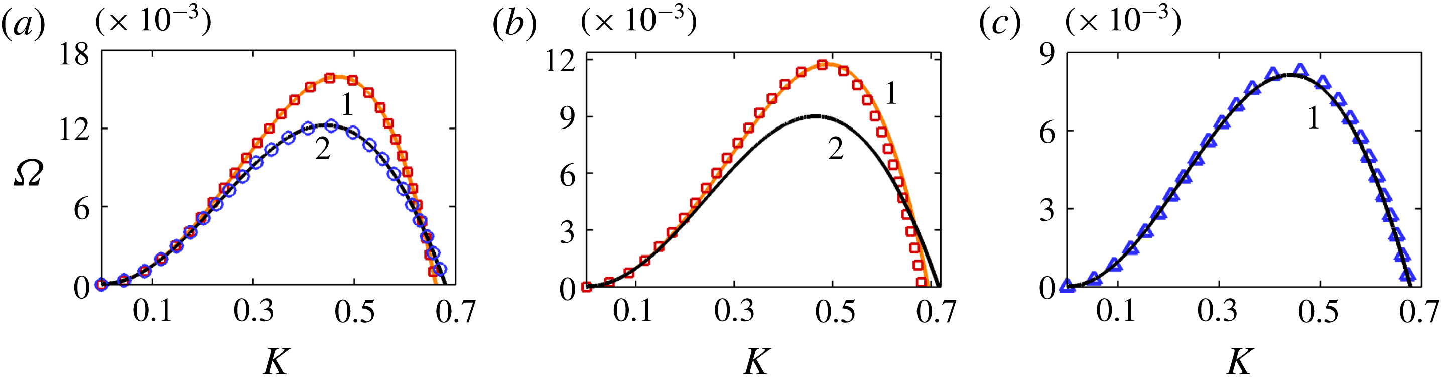
Typical parametric values used in the calculations for the nematic film (Stephen & Straley Reference Stephen and Straley1974; de Gennes & Prost Reference de Gennes and Prost1993; Stewart Reference Stewart2004).

7.2 Importance of GLSA, dielectric anisotropy, and bulk elasticity
A series of
 $\unicode[STIX]{x1D6FA}$
versus
 $K$
plots in the following figure 3 highlight the usefulness as well as limitations of the long-wave analysis with the change in the anchoring near the boundaries. Further, figures 4 and 5 show the effects of thermodynamic parameters, such as dielectric anisotropy
 $(\unicode[STIX]{x1D716}_{d})$
and Frank bulk elastic constant
 $(K_{f})$
, and kinetic parameters, such as the Leslie viscosity coefficients
 $(\unicode[STIX]{x1D6FC}_{i})$
, on the length and the time scales of the electric-field-induced instabilities of thin NLC films. However, before we discuss these aspects, an analysis on the following expressions of the normal and tangential stress balance in (3.8) and (3.9) at the NI interface can provide useful insights into understanding the different forces responsible for the interfacial deformation of NLC films under an electric field,
 $$\begin{eqnarray}\displaystyle & & \displaystyle P-P_{0}+E_{r}^{-1}\unicode[STIX]{x1D703}_{,Z}^{2}-(D_{1}U_{,X}+D_{2}U_{,Z}+D_{3}W_{,X}+D_{4}W_{,Z})\nonumber\\ \displaystyle & & \displaystyle \quad +\,[[\unicode[STIX]{x1D716}_{d}(\sin 2\unicode[STIX]{x1D703}H_{,X}-\cos ^{2}\unicode[STIX]{x1D703})-\unicode[STIX]{x1D716}_{\bot }]\unicode[STIX]{x1D6F9}_{,Z}^{2}+\unicode[STIX]{x1D6F9}_{a,Z}^{2}]=-\unicode[STIX]{x1D6E4}H_{,XX},\end{eqnarray}$$
 $$\begin{eqnarray}E_{r}^{-1}(\unicode[STIX]{x1D703}_{,Z}^{2}H_{,X}+\unicode[STIX]{x1D703}_{,X}\unicode[STIX]{x1D703}_{,Z})-(B_{1}U_{,X}+B_{2}U_{,Z}+B_{3}W_{,X}+B_{4}W_{,Z})=0.\end{eqnarray}$$
For example, the third term in the expression of normal stress balance (7.1) is known as the Frank bulk elasticity
 $(\unicode[STIX]{x1D6F1}_{ES})$
(Vandenbrouck et al.
Reference Vandenbrouck, Valignat and Cazabat1999), which together with the surface tension term in the right-hand side restricts any interfacial deformation of an NLC film. The bracketed fourth term in this expression is the nematodynamic components of the normal stress balance having the Leslie viscosity coefficients, while the bracketed fifth term corresponds to the destabilizing EHD stress
 $(\unicode[STIX]{x1D6F1}_{EF})$
. Equation (7.1) clearly indicates that NLC films with
 $\unicode[STIX]{x1D716}_{d}>0$
or
 $\unicode[STIX]{x1D716}_{d}<0$
are expected show a very different type of EHD instability as compared to the same observed for isotropic films
 $(\unicode[STIX]{x1D716}_{d}=0)$
. The other important parameter to notice is the bracketed first term in the expression of tangential stress balance (7.2) corresponding to the elastic Ericksen stress (de Gennes & Prost Reference de Gennes and Prost1993), which facilitates the interfacial deformation of an NLC film. The bracketed second term in (7.2) shows nematodynamic components of the tangential stress balance having Leslie viscosity coefficients. Equations (7.1) and (7.2) together suggest that the interfacial deformation of a thin nematic film under the influence of an electric field can be significantly different from the same of an isotropic film owing to the presence of the additional stabilizing term originating from the Frank elasticity and the destabilizing terms originating from the anisotropic EHD and Ericksen stresses. In the following discussions, the base-state expressions for anisotropic EHD force per unit volume
 $(F_{EF}=\unicode[STIX]{x1D6F1}_{EF,Z})$
and elastic Ericksen force per unit volume
 $(F_{ES}=\unicode[STIX]{x1D6F1}_{ES,Z})$
have been used to estimate the strength of the destabilizing influences at the NI interface in the presence of an electric field and analyse the GLSA results,
 $$\begin{eqnarray}\displaystyle & \displaystyle F_{EF}=[2\unicode[STIX]{x1D6F9}_{a,Z}\unicode[STIX]{x1D6F9}_{a,ZZ}+\unicode[STIX]{x1D716}_{d}\sin 2\unicode[STIX]{x1D703}\hspace{2.22198pt}\unicode[STIX]{x1D6F9}_{,Z}^{2}\unicode[STIX]{x1D703}_{,Z}-2(\unicode[STIX]{x1D716}_{\bot }+\unicode[STIX]{x1D716}_{d}\cos ^{2}\unicode[STIX]{x1D703})\unicode[STIX]{x1D6F9}_{,Z}\unicode[STIX]{x1D6F9}_{,ZZ}], & \displaystyle\end{eqnarray}$$
 $$\begin{eqnarray}\displaystyle & \displaystyle F_{ES}=2E_{r}^{-1}\unicode[STIX]{x1D703}_{,Z}\unicode[STIX]{x1D703}_{,ZZ}. & \displaystyle\end{eqnarray}$$
Comparison of LWLSA (lighter shade, curve 1) and GLSA (darker shade, curve 2) curves for the variation of growth coefficient
 $(\unicode[STIX]{x1D6FA})$
with wavenumber
 $(K)$
of a nematic film for different filling ratios,
 $\unicode[STIX]{x1D708}=h_{0}/d=1/D$
. In (a–d) column i shows the nematic films with homeotropic–homeotropic (H–H,
 $\unicode[STIX]{x1D703}_{1}$
and
 $\unicode[STIX]{x1D703}_{2}=0^{\circ }$
), homeotropic–planar (H–P,
 $\unicode[STIX]{x1D703}_{1}=0^{\circ }$
and
 $\unicode[STIX]{x1D703}_{2}=90^{\circ }$
), planar–homeotropic (P–H,
 $\unicode[STIX]{x1D703}_{1}=90^{\circ }$
and
 $\unicode[STIX]{x1D703}_{2}=0^{\circ }$
), and planar–planar (P–P,
 $\unicode[STIX]{x1D703}_{1}$
and
 $\unicode[STIX]{x1D703}_{2}=90^{\circ }$
) director orientations, respectively, at the NS and NI boundaries. Columns ii, iii, and iv are plots for
 $\unicode[STIX]{x1D708}=0.25$
, 0.5, and 0.75, respectively, with
 $\unicode[STIX]{x1D716}_{d}=0.5$
. The other necessary parameters for the plots are shown in table 1.

The results from GLSA when the dielectric anisotropy
 $(\unicode[STIX]{x1D716}_{d})$
and Frank bulk elastic constant
 $(K_{f})$
of the NLC film are varied. The solid curve ‘
 $i$
’ (lighter shade) shows a comparative plot for an isotropic film deforming under electric field. (
 $a$
i–
 $d$
i) Show the NLC films with H–H, H–P, P–H, and P–P director orientations, respectively, at the NS and NI boundaries. In (
 $a$
ii–
 $c$
ii) the curves 1–3 (darker shade) represent
 $\unicode[STIX]{x1D716}_{d}=-0.7$
, 0, and 5, respectively, when
 $\unicode[STIX]{x1D716}_{\bot }=6$
and
 $\unicode[STIX]{x1D708}=0.75$
. In (
 $d$
ii), the curves 1–3 (darker shade) represent
 $\unicode[STIX]{x1D716}_{\bot }=5$
, 6, and 7, respectively, when
 $\unicode[STIX]{x1D716}_{\Vert }$
= 10 and
 $\unicode[STIX]{x1D708}=0.75$
, and the curve ‘
 $i$
’ (lighter shade) corresponds to an isotropic film having
 $\unicode[STIX]{x1D716}_{i}=6$
. Column iii corresponds to the filling ratio
 $\unicode[STIX]{x1D708}=0.25$
in which the curves 1–3 (darker shade) correspond to
 $K_{f}=3$
pN, 9 pN, and 15 pN, respectively, when
 $\unicode[STIX]{x1D716}_{d}=5$
. The other necessary parameters for the plots are shown in table 1.

The GLSA plots showing the influence of Leslie viscosity coefficients
 $(\unicode[STIX]{x1D6FC}_{i})$
. Panels (
 $a$
i–
 $d$
i) show the NLC films with H–H, H–P, P–H, and P–P director orientations at the NS and NI boundaries. Panels (
 $a$
ii–
 $d$
ii) correspond to
 $K_{f},\unicode[STIX]{x1D6FC}_{4},\unicode[STIX]{x1D6FC}_{1}\neq 0$
and
 $\unicode[STIX]{x1D6FC}_{2},\unicode[STIX]{x1D6FC}_{3},\unicode[STIX]{x1D6FC}_{5}=0$
in which the curves 1–3 represent
 $\unicode[STIX]{x1D6FC}_{1}=0.003$
Pa s, 0.006 Pa s, and 0.009 Pa s, respectively. Panels (
 $a$
iii–
 $d$
iii) correspond to
 $K_{f},\unicode[STIX]{x1D6FC}_{4},\unicode[STIX]{x1D6FC}_{2}\neq 0$
and
 $\unicode[STIX]{x1D6FC}_{1},\unicode[STIX]{x1D6FC}_{3},\unicode[STIX]{x1D6FC}_{5}=0$
where curves 1–3 represent
 $\unicode[STIX]{x1D6FC}_{2}=-0.007$
Pa s,
 $-0.014$
Pa s, and
 $-0.021$
Pa s, respectively. Panels (
 $a$
iv–
 $d$
iv) correspond to
 $K_{f},\unicode[STIX]{x1D6FC}_{4},\unicode[STIX]{x1D6FC}_{3}\neq 0$
and
 $\unicode[STIX]{x1D6FC}_{1},\unicode[STIX]{x1D6FC}_{2},\unicode[STIX]{x1D6FC}_{5}=0$
in which curves 1–3 represent
 $\unicode[STIX]{x1D6FC}_{3}=-0.001$
Pa s,
 $-0.004$
Pa s, and
 $-0.007$
Pa s, respectively. Panels (
 $a$
v–
 $d$
v) correspond to
 $K_{f},\unicode[STIX]{x1D6FC}_{4},\unicode[STIX]{x1D6FC}_{5}\neq 0$
and
 $\unicode[STIX]{x1D6FC}_{1},\unicode[STIX]{x1D6FC}_{2},\unicode[STIX]{x1D6FC}_{3}=0$
in which curves 1–3 represent
 $\unicode[STIX]{x1D6FC}_{5}=0.03$
Pa s, 0.05 Pa s, and 0.07 Pa s, respectively. The other necessary parameters for the plots are shown in table 1.

An extensive comparison between analytical eigenvalues obtained from the LWLSA (orange or lighter shade) and the numerical eigenvalues obtained from the GLSA (black or darker shade) has also been carried out for the electric-field-induced instabilities of the LC films, as summarized in figure 3. The first column of panels (a–d) schematically show the typical director orientations considered inside the NLC films such as homeotropic–homeotropic (H–H,
 $\unicode[STIX]{x1D703}_{1}$
and
 $\unicode[STIX]{x1D703}_{2}=0^{\circ }$
), homeotropic–planar (H–P,
 $\unicode[STIX]{x1D703}_{1}=0^{\circ }$
and
 $\unicode[STIX]{x1D703}_{2}=90^{\circ }$
), planar–homeotropic (P–H,
 $\unicode[STIX]{x1D703}_{1}=90^{\circ }$
and
 $\unicode[STIX]{x1D703}_{2}=0^{\circ }$
), and planar–planar (P–P,
 $\unicode[STIX]{x1D703}_{1}$
and
 $\unicode[STIX]{x1D703}_{2}=90^{\circ }$
), respectively, at the NS and NI boundaries. The remaining columns in the figure correspond to NLC films with different NLC to air filling ratios between the electrodes
 $(\unicode[STIX]{x1D708}=h_{0}/d)$
undergoing EHD instabilities.
The plots suggest that the analytical eigenvalues match fairly well with the numerical ones in the long-wave limit,
 $(K\rightarrow 0)$
. However, in the plots (
 $b$
ii), (
 $c$
ii), (
 $a$
iii), and (
 $a$
iv–
 $d$
iv), the difference in the analytical and numerical eigenvalues become prominent at larger values of
 $K$
. Panels (a,d) show that when the director orientation across the nematic film is uniform
 $(\unicode[STIX]{x1D703}_{,Z}=0)$
, the LWLSA and GLSA eigenvalues matched fairly well at smaller filling ratios
 $\unicode[STIX]{x1D708}\leqslant 0.5$
when the EHD stress at the NI interface is relatively weaker. However, at higher filling ratios,
 $\unicode[STIX]{x1D708}\geqslant 0.5$
, as the EHD stress at the NI interface become relatively stronger the eigenvalues obtained from the GLSA deviate significantly from the same obtained from the LWLSA. It may be noted here that this phenomenon is true even for an isotropic film, as reported by a number of previous works (Bandyopadhyay et al.
Reference Bandyopadhyay, Sharma, Thiele and Reddy2009). The results from this figure show that at higher field intensities the EHD instabilities of thin films require GLSA rather than LWLSA for accurate predictions of the eigenvalues corresponding to the unstable modes. The deviation of LWLSA from GLSA is more prominent when the director orientation across the film is non-uniform
 $(\unicode[STIX]{x1D703}_{,Z}\neq 0)$
, as shown by the plots in panels (b,c).
Figure 4 shows the typical
 $\unicode[STIX]{x1D6FA}$
versus
 $K$
plots when the dielectric anisotropy
 $(\unicode[STIX]{x1D716}_{d})$
and bulk elastic constant
 $(K_{f})$
are varied. Again, panels (
 $a$
i–
 $d$
i) schematically show the typical director orientations H–H, H–P, P–H, and P–P at the NS and NI boundaries of the NLC films. Panels (
 $a$
ii–
 $d$
ii) show the effects of
 $\unicode[STIX]{x1D716}_{d}$
, and panels (
 $a$
iii–
 $d$
iii) show the effect of
 $K_{f}$
. Panels (
 $a$
ii–
 $c$
ii) suggest that as compared to an isotropic film (curve ‘
 $i$
’), the NLC film with isotropic dielectric properties (curve 2,
 $\unicode[STIX]{x1D716}_{d}=0$
) is always more stable owing to the reduction in the magnitude of the dominant growth coefficient
 $(\unicode[STIX]{x1D6FA}_{m})$
. In this situation, the destabilizing forces have to overcome the additional Frank bulk elasticity of the NLC film, which leads to larger time (smaller
 $\unicode[STIX]{x1D6FA}_{m}$
) and length (smaller
 $K_{m}$
) scales of instability as compared to a purely isotropic film. A comparison between curves 1 and 2 suggests that the dominant length
 $(\unicode[STIX]{x1D6EC}_{m}=2\unicode[STIX]{x03C0}/K_{m})$
and time
 $(1/\unicode[STIX]{x1D6FA}_{m})$
scales can be significantly larger for NLC films with negative
 $(\unicode[STIX]{x1D716}_{d}<0)$
dielectric anisotropy than NLC films with an isotropic dielectric property. In contrast, curves 2 and 3 suggest that the dominant length and time scales can be significantly smaller for NLC films with positive
 $(\unicode[STIX]{x1D716}_{d}>0)$
dielectric anisotropy as compared to NLC films with an isotropic dielectric property. The condition
 $\unicode[STIX]{x1D716}_{d}>0$
ensures an easier alignment of the NLC molecules and subsequent charge separation near the NI and NS interfaces along the direction of the applied electric field, which facilitates the electric-field-induced deformation of the NI interface. Whereas, for the condition
 $\unicode[STIX]{x1D716}_{d}<0$
, the induced charge separation in the normal direction of the applied electric field acts against the electric-field-induced deformation of the NI interface.
Panels (
 $a$
ii–
 $d$
ii) also show that the director orientations at the NI and NS interfaces play crucial roles in modulating the dominant time and length scales of the EHD instabilities. For example, when all the molecules are oriented towards the direction of the electric field and
 $\unicode[STIX]{x1D716}_{d}>0$
[curve 3 in panel (
 $a$
ii)], smaller time and length scales of instability are observed. In fact, when the molecules at the NI interface are oriented in the direction of the electric field [curve 3 in panel (
 $c$
ii)], we observe similar length and time scales of instability as observed for the case in the plot (
 $a$
ii). Panels (
 $a$
ii) and (
 $c$
ii) together suggest that the anchoring condition at the NI (NS) interface has more (less) significance on the length and time scales of the EHD instabilities of the NLC films. In comparison, curve 3 of panels (
 $b$
ii) and (
 $d$
ii) show that when the director orientation is planar at the NI interface, the length and time scales are much larger than the aforementioned cases because of the larger expense of EHD stresses for orienting the molecules towards the direction of the electric field.
The curves in panels (
 $a$
iii–
 $d$
iii) show the effect of Ericksen stress on the dominant length and time scales of the electric field induced instabilities of the NLC films. Previously, (7.1) and (7.2) suggested that the effect of Ericksen stress is a function of the director orientation along the nematic axis
 $(\unicode[STIX]{x1D703}_{,Z})$
. Thus, a uniform director orientation
 $(\unicode[STIX]{x1D703}_{,Z}=0)$
across the film is expected to show negligible influence of Ericksen stress, as can be observed in panels (
 $a$
iii) and (
 $d$
iii). However, panels (
 $b$
iii) and (
 $c$
iii) suggest that when there is a variation in
 $\unicode[STIX]{x1D703}_{,Z}$
across the film, the Ericksen stress can have a significant destabilizing influence. For example, when the films are thinner (
 $\unicode[STIX]{x1D708}=0.25$
), the destabilizing effect of the Ericksen elastic stress is more pronounced at larger values of
 $\unicode[STIX]{x1D703}_{,Z}$
near the NI interface. In such a situation, the dominant length and time scales reduce and the destabilizing effect enhances with an increase in the magnitude of
 $K_{f}$
, as shown by curves 1–3.
Apart from the previously discussed thermodynamic parameters, kinetic parameters such as the Leslie viscosity coefficients (
 $\unicode[STIX]{x1D6FC}_{i}$
where
 $i=1$
, 2, 3, and 5) can also have some influence on the electric-field-induced instabilities of the NLC films. In figure 5, panels (
 $a$
i–
 $d$
i) show nematic films with H–H, H–P, P–H, and P–P anchoring conditions at the NS and NI boundaries, while the renaining panels show the effects of
 $\unicode[STIX]{x1D6FC}_{i}$
under different anchoring conditions at the NI and NS interfaces. It may be noted here that
 $\unicode[STIX]{x1D6FC}_{4}/2$
is the Newtonian viscosity of the films and has a finite value in all the plots. The plots suggest that the Leslie viscosity coefficients can change the magnitude of the dominant time scale of the EHD instabilities of thin nematic films. Further, the plots suggest that the effects of
 $\unicode[STIX]{x1D6FC}_{2}$
and
 $\unicode[STIX]{x1D6FC}_{5}$
are more pronounced than the others. Importantly, all the Leslie viscosity coefficients do not influence the length scale, as previously observed for other kinetic parameters such as the viscosity and relaxation time of a viscous or viscoelastic film (Tomar et al.
Reference Tomar, Shankar, Shukla, Sharma and Biswas2006; Bandyopadhyay, Reddy & Sharma Reference Bandyopadhyay, Reddy and Sharma2012). However, a comparison between the GLSA and LWLSA results also suggests that the effects of the terms associated with the Leslie viscosity coefficients (
 $B_{i}$
and
 $D_{i}$
) in the (7.1) and (7.2) can be significant and should be included in analysing the stability of NLC thin films. For example, the differences in the dominant time scale obtained for the LWLSA and GLSA in figure 3 can be attributed to the presence (absence) of the Leslie viscosity coefficients in the GLSA (LWLSA).
In brief, figures 3–5 reveal quite a few interesting facts related to the electric-field-induced instabilities of thin NLC films. Firstly, they show the effects of thermodynamic parameters such as the dielectric anisotropy, Frank bulk elasticity, and Ericksen elastic stress on tuning the time and length scales of such instabilities. Secondly, they emphasize the importance of GLSA over LWLSA to uncover the diverse stability paradigms. Lastly, the plots show the effects of the director orientations across the film, anchoring conditions near the interfaces, and Leslie viscosity coefficients while analysing such instabilities.
7.3 Different EHD modes from GLSA
Most of the previous theoretical works on the free surface instabilities of thin NLC films could only predict the presence of the long-wave (LW) interfacial mode owing to the use of lubrication approximations in the analyses (Ben Amar & Cummings Reference Ben Amar and Cummings2001; Cummings Reference Cummings2004; Cummings, Lin & Kondic Reference Cummings, Lin and Kondic2011; Lin et al.
Reference Lin, Cummings, Archer, Kondic and Thiele2013a
,Reference Lin, Kondic, Thiele and Cummings
b
). In the previous section, we have highlighted the limitations of the LWLSA over the GLSA in predicting the unstable modes of the electric field induced instabilities of NLC films even in that limit. Importantly, the discussions on the figures 2–5 are largely restricted to uncovering the LW modes of such instabilities employing the proposed GLSA. However, many recent experimental studies have predicted the presence of multiple instability modes for NLC films under the influence of an external electric field (Oswald Reference Oswald2010a
,Reference Oswald
b
). Herein, the proposed GLSA is able to predict the existence of finite-wavenumber (FW) modes alongside the LW modes for the electric-field-induced free surface instabilities of NLC films. Since the major focus of this study is to identify the influence of the electric field, Ericksen stress, dielectric anisotropy, and Frank bulk elasticity of the NLC film on the mode selection, we restrict our study to a few dimensionless parameters such as
 $E_{r}$
, the gradient of the director angle
 $(\unicode[STIX]{x1D703}_{,Z})$
, the filling ratio
 $(\unicode[STIX]{x1D708})$
, and the dielectric anisotropy
 $(\unicode[STIX]{x1D716}_{d})$
. The following insights on these parameters can elucidate discussions associated with the following figures. For example, a higher value of
 $E_{r}$
signifies either exposure to a strong electric field or a weak Frank bulk elasticity inside the NLC film. Similarly, a higher (lower) value of
 $\unicode[STIX]{x1D703}_{,Z}$
near the NI interface signifies the presence of a strong (weak) destabilizing Ericksen stress, which may facilitate (impede) the free surface deformations of the NLC films. In contrast, a higher value of
 $\unicode[STIX]{x1D703}_{,Z}$
inside the film with larger values of
 $K_{f}$
can also empower the restoring influence of Frank bulk elasticity, which may restrict any free surface deformation of the NLC films. A higher value of
 $\unicode[STIX]{x1D716}_{d}$
ensures easy alignment of NLC molecules towards the direction of the electric field while a higher
 $\unicode[STIX]{x1D708}$
ensures a higher EHD stress at the NI interface to facilitate deformation.
The GLSA results of a nematic film with H–H (
 $\unicode[STIX]{x1D703}_{1}=0^{\circ }$
and
 $\unicode[STIX]{x1D703}_{2}=0^{\circ }$
) orientations at the NS and NI boundaries when
 $\unicode[STIX]{x1D708}=0.75$
. (a) Variation of the director orientation at the base state
 $(\bar{\unicode[STIX]{x1D703}})$
along the
 $Z$
-axis as schematically also shown by the diagram S1. (b) Typical
 $\unicode[STIX]{x1D6FA}$
versus
 $K$
curves for this case, where curves 1–5 represent
 $E_{r}=354.2$
, 796.9, 1416.6, 2213.5, and 3187.4, respectively, when
 $\unicode[STIX]{x1D716}_{d}=9$
. (c,d) Variations of
 $\unicode[STIX]{x1D6FA}_{m}$
and
 $\unicode[STIX]{x1D6EC}_{m}$
with
 $E_{r}$
and
 $\unicode[STIX]{x1D716}_{d}$
, respectively. In (c)
 $K_{f}=5$
pN and
 $\unicode[STIX]{x1D716}_{d}=9$
, whereas in
 $(d)~E_{r}=2213.5$
. The other essential parameters used for these plots are shown in table 1.

We initiate the discussions with the situation when the NS and NI interfaces of the NLC film has H–H anchoring conditions, as shown in figure 6(a). Clearly, the director orientations across the NLC film ensure the absence of the Ericksen elastic stress and Frank bulk elasticity because
 $\unicode[STIX]{x1D703}_{,Z}=0$
. Thus, in this case, panel (b) shows the presence of the LW mode of instability only, which has similarity with the electric field induced instabilities of the isotropic thin films (Schäffer et al.
Reference Schäffer, Thurn-Albrecht, Russell and Steiner2000; Verma et al.
Reference Verma, Sharma, Kargupta and Bhaumik2005). Panels (c,d) show the variations in
 $\unicode[STIX]{x1D6FA}_{m}$
and
 $\unicode[STIX]{x1D6EC}_{m}$
with
 $E_{r}$
and
 $\unicode[STIX]{x1D716}_{d}$
, respectively. Panels (b–d) together suggest that the dominant length and time scales of the LW mode reduce with increasing strength of the destabilizing electric field (higher
 $E_{r}$
) and increasing dielectric anisotropy of the film (higher
 $\unicode[STIX]{x1D716}_{d}$
).
The results obtained from GLSA of an NLC film (
 $\unicode[STIX]{x1D716}_{d}$
= 9 and
 $\unicode[STIX]{x1D708}=0.75$
) with H–A (
 $\unicode[STIX]{x1D703}_{1}=0^{\circ }$
and
 $\unicode[STIX]{x1D703}_{2}=45^{\circ }$
) director orientations at the NS and NI boundaries. (a) Variations of
 $\bar{\unicode[STIX]{x1D703}}$
at the base state along the
 $Z$
-axis with
 $E_{r}$
, as schematically shown in diagram S1. The curves 1 (blue) and 6 (green) represent
 $E_{r}=3689.2$
and 11067.5, respectively. (b) Variation of
 $\unicode[STIX]{x1D6FA}$
with
 $K$
corresponding to panel (a) to depict the transition from unimodal (curve 1 – LW mode, blue) to bimodal (curve 6 – both LW and FW modes, green). The curves 2–5 represent
 $E_{r}=6148.6$
(black), 7378.3 (orange), 8513.5 (olive), and 10061.4 (red), respectively. (c–f) Variations of
 $F_{EF}$
,
 $F_{ES}$
,
 $\unicode[STIX]{x1D6FA}_{m}$
, and
 $\unicode[STIX]{x1D6EC}_{m}$
with
 $E_{r}$
when
 $\unicode[STIX]{x1D6F9}_{0}=50$
V and
 $K_{f}=1$
pN. The other necessary parameters for these plots are shown in table 1.

Figure 7 shows the GLSA results when the director fields at the NS and NI interfaces have homeotropic–angular orientations (H–A,
 $\unicode[STIX]{x1D703}_{1}=0^{\circ }$
and
 $\unicode[STIX]{x1D703}_{2}=45^{\circ }$
), as schematically shown in the diagram S1 of panel (a). Panel (a) shows the variation in the director orientation
 $(\bar{\unicode[STIX]{x1D703}})$
across the film while panel (b) shows the variation of
 $\unicode[STIX]{x1D6FA}$
with
 $K$
at different values of
 $E_{r}$
. Curve 1 in panels (a,b) suggests that when the variation in the director orientation
 $(\unicode[STIX]{x1D703}_{,Z})$
near the NI interface is relatively small the instability manifests by the LW mode. Curves 2–5 in panel (b) suggest that with a progressive increase in
 $E_{r}$
an additional FW mode of instability appears at higher wavenumbers. Curves 1 and 6 in panel (a) suggest that the magnitude of
 $\unicode[STIX]{x1D703}_{,Z}$
near the NI interface increases with
 $E_{r}$
because the NLC molecules in the bulk orient more in the direction of the applied electric field at higher electric field strength
 $(\unicode[STIX]{x1D713}_{0})$
, whereas molecules at the boundary retain their orientation as enforced in the boundary condition. In such a situation, the dominant time (reduction in
 $\unicode[STIX]{x1D6FA}_{m}$
) and length (increase in
 $\unicode[STIX]{x1D6EC}_{m}$
) scales are found to increase because of the increase in the bulk elasticity of the NLC film (third term in (7.1)), as shown by curves 2–4 in panel (b). However, curves 4 and 5 in panel (b) suggest that, beyond a critical value of
 $E_{r}=E_{r}^{c}$
, an increase in the Ericksen stress near the NI interface fuels up the FW mode of instability. Panels (c,e) show the increase in the force per unit volume associated with the Ericksen stress (
 $F_{,ES}$
, equation (7.4)) with
 $E_{r}$
. In this case, the sharp increase in
 $\unicode[STIX]{x1D703}_{,Z}$
and
 $\unicode[STIX]{x1D703}_{,ZZ}$
near
 $Z=1$
dominates the decaying nature of
 $F_{ES}$
with
 $E_{r}^{-1}$
. The plots also indicate the progressive decrease in the EHD force
 $(F_{EF})$
with
 $E_{r}$
progressively makes the LW mode a subdominant mode while the FW mode becomes the dominant mode. The broken lines in panels (d,f) suggest that in this case the dominant length and time scales corresponding to the LW mode progressively increase with
 $E_{r}$
. In comparison, the solid lines in these plots suggest that after the appearance (e.g. for panels (d,f),
 $E_{r}^{c}=6510.3$
and 8570.7, respectively) a progressive reduction in the time and length scales for the FW instability with increasing
 $E_{r}$
.
Importantly, the LW mode is the dominant mode at lower values of
 $E_{r}$
where the instability showed unimodal
 $\unicode[STIX]{x1D6FA}$
versus
 $K$
curves in panel (b). In comparison, at moderately high values of
 $E_{r}$
, bimodal
 $\unicode[STIX]{x1D6FA}$
versus
 $K$
plots are observed in which the LW mode is still dominant while the FW mode is the subdominant mode. The FW (LW) mode becomes the dominant (subdominant) mode beyond a threshold value of
 $E_{r}$
. The LW (FW) mode fuelled up by the external electric field (Ericksen Stress) is progressively shifted towards the longer- (shorter-)wavelength regime while the intermediate wavenumber showed stability under the influence of the Frank bulk elasticity inside the NLC film.
Neutral stability curves obtained from GLSA of an NLC film with H–A (
 $\unicode[STIX]{x1D703}_{1}=0^{\circ }$
and
 $\unicode[STIX]{x1D703}_{2}=45^{\circ }$
) orientations at the NS and NI boundaries. (a–d) Variation of critical wavenumber
 $(K)$
with
 $E_{r}$
when
 $\unicode[STIX]{x1D713}_{0}=50$
V,
 $E_{r}$
when
 $K_{f}=1$
pN,
 $\unicode[STIX]{x1D708}$
when
 $\unicode[STIX]{x1D716}_{d}=9$
, and
 $\unicode[STIX]{x1D716}_{d}$
when
 $\unicode[STIX]{x1D708}=0.75$
, respectively.
 $\unicode[STIX]{x1D716}_{d}$
and
 $\unicode[STIX]{x1D708}$
are kept constant at
 $\unicode[STIX]{x1D716}_{d}=9$
and
 $\unicode[STIX]{x1D708}=0.75$
for panels (a,b) whereas
 $E_{r}=11067.5$
is kept constant for panels (c,d). Other parameters used for these plots are shown in table 1.

Neutral stability curves for the NLC film discussed in figure 7 are presented in figure 8. Panels (a–d) show the variations in the critical wavenumber
 $(K)$
with
 $E_{r}$
at constant
 $\unicode[STIX]{x1D713}_{0}$
,
 $E_{r}$
at constant
 $K_{f}$
,
 $\unicode[STIX]{x1D708}$
, and
 $\unicode[STIX]{x1D716}_{d}$
, respectively. In all these plots, the wavenumbers corresponding to the FW mode are enclosed by the solid lines between the neutral wavenumbers
 $K_{1}^{F}$
and
 $K_{2}^{F}$
, whereas the same for the LW modes are enclosed by the broken lines having neutral wavenumbers
 $K_{1}^{L}$
and
 $K_{2}^{L}$
. Panel (a) shows the presence of LW until
 $E_{r}^{c}$
, and beyond this limit the additional FW mode appears, as previously discussed in figure 7. Panels (a,b) together show that the FW mode can be fuelled up either by reducing the bulk elasticity of the NLC film or by increasing the external field strength. Further, panels (c,d) show even increasing
 $\unicode[STIX]{x1D708}$
and
 $\unicode[STIX]{x1D716}$
for an NLC film can cause the transition from unimodal to bimodal instability for NLC films under exposure to an electric field.
In brief, figures 6–8 together highlight that a competition between the restoring Frank bulk elasticity of the NLC films with the destabilizing Ericksen stress near the NI interface can fuel up bimodal LW and FW modes of instability. A dominant LW mode prevails when the influence of the bulk elasticity of the NLC films is more prominent and only the electric field can destabilize the free surface of the NLC film. In comparison, the FW mode is dominant when the combined effects of the Ericksen and EHD stresses are more pronounced.
The results from GLSA of an NLC film with H–P orientation (
 $\unicode[STIX]{x1D703}_{1}=0^{\circ }$
and
 $\unicode[STIX]{x1D703}_{2}=90^{\circ }$
) at the NS and NI boundaries. (a,c) Variations of
 $\bar{\unicode[STIX]{x1D703}}$
along the
 $Z$
-axis when
 $\unicode[STIX]{x1D716}_{d}=9$
and
 $-0.1$
, respectively, and
 $E_{r}=3689.2$
, also schematically shown by the diagram S1 in both the plots. (b,d) Variation of
 $\unicode[STIX]{x1D6FA}$
with
 $K$
. Curve 1 of both (b) (green) and (d) (olive) correspond to curve 1 of (a) (green) and (c) (olive), respectively. Curve 2 of (b) (red) represents
 $E_{r}=1106.8$
and
 $\unicode[STIX]{x1D716}_{d}=9$
, and curve 2 of (d) (blue) represents
 $E_{r}=3689.2$
and
 $\unicode[STIX]{x1D716}_{d}=-0.5$
, when
 $\unicode[STIX]{x1D708}=0.75$
. Other parameters used for these plots are shown in table 1.

Figure 9 shows GLSA results for an NLC film with H–P orientation at the NS and NI interfaces as shown in panel (a). Panel (a) also shows that for the condition
 $\unicode[STIX]{x1D716}_{d}>0$
more molecules are oriented along the direction of the electric field except in the immediate vicinity of the NI interface, where a sharp change of director orientation takes place from homeotropic to planar, causing a large value of Ericksen stress at higher field intensities. Panel (b) shows a transition of modes from unimodal (curve 2) to bimodal (curve 1) with increasing
 $E_{r}$
. In comparison, panel (c) shows that when
 $\unicode[STIX]{x1D716}_{d}<0$
the molecules are mostly oriented along the normal direction to the applied field except for the zone near the NS interface, where a sharp change of director orientation takes place from planar to homeotropic. Importantly, the uniform planar orientations in the near vicinity of the NI interface subdue the Ericksen stress even at higher field intensities. Thus, in this situation, only the LW mode of instability is observed when
 $\unicode[STIX]{x1D716}_{d}<0$
, as shown by curves 1 and 2 in panel (d).
Briefly, figures 6–9 reveal that an NLC film with positive dielectric anisotropy can show a bimodal instability when the combined effects of the Ericksen and EHD stresses subdue the Frank bulk elasticity and the surface tension forces. The figures also suggest that films with negative dielectric anisotropy and larger magnitudes of Frank bulk elasticity can only show the LW interfacial mode, especially when the magnitude of the Ericksen stress is small across the film.
7.4 Fréedericksz-type transition for NLC films
Interestingly, the GLSA can also predict a Fréedericksz-type transition (FTT) (Fraden & Meyer Reference Fraden and Meyer1986; Kuzma Reference Kuzma1986; Chandrasekhar Reference Chandrasekhar1992; de Gennes & Prost Reference de Gennes and Prost1993; Müller & Brand Reference Müller and Brand2005) when the director fields at the NS and NI interfaces are in P–P anchoring conditions. The FTT is in general observed when an LC film is sandwiched between a pair of electrodes and under the influence of an external electric field. In such a situation, the uniform director field
 $(\unicode[STIX]{x1D703}_{,Z}=0)$
across the film transforms into a non-uniform
 $(\unicode[STIX]{x1D703}_{,Z}\neq 0)$
field across the film beyond a critical strength of external magnetic or electric field (Chandrasekhar Reference Chandrasekhar1992; de Gennes & Prost Reference de Gennes and Prost1993; Müller & Brand Reference Müller and Brand2005). However, the GLSA uncovers that a similar FTT can also be observed for an NLC film with a free deformable surface. For the NLC films with a free surface, the FTT is expected to occur simultaneously with the free surface deformation, which makes the phenomenon somewhat different from the same when the NLC film is confined between a pair of rigid electrodes. Figure 10 shows results from the GLSA when the director fields at the NS and NI interfaces are in P–P anchoring conditions. The schematic diagrams S1 and S2 show the orientations of the molecules across the NLC film before and after the transition. Curves 1 and 2 in panel (a) also show the variation in the base-state orientation of the NLC molecules across the film. Panels (b,d) together show the sole existence of the LW mode at lower values of
 $E_{r}$
when the orientations of all the molecules across the film are planar
 $(\unicode[STIX]{x1D703}_{,Z}=0)$
. However, at higher values of
 $E_{r}$
there is a transition of orientations of the molecules across the film, as depicted by the schematic diagrams and the curves in panel (a). In such a situation,
 $\unicode[STIX]{x1D703}_{,Z}$
near the NI interface becomes finite, which causes the Ericksen stress to fuel up the FW mode alongside the LW mode.
GLSA results of an NLC film with P–P orientations (
 $\unicode[STIX]{x1D703}_{1}=90^{\circ }$
and
 $\unicode[STIX]{x1D703}_{2}=90^{\circ }$
) at the NS and NI boundaries when
 $\unicode[STIX]{x1D716}_{d}=9$
and
 $\unicode[STIX]{x1D708}=0.75$
. (a) Curves 1 (blue) and 2 (olive) show the variation of
 $\bar{\unicode[STIX]{x1D703}}$
along the
 $Z$
-axis at
 $E_{r}=3543.1$
and 3689.2, which is also schematically shown by the diagrams S1 and S2. (b) Curves 1 (blue) and 2 (olive) show the variation of
 $\unicode[STIX]{x1D6FA}$
with
 $K$
corresponding to (a). (c,d) Variations of
 $F_{EF}$
,
 $F_{ES}$
,
 $\unicode[STIX]{x1D6FA}_{m}$
, and
 $\unicode[STIX]{x1D6EC}_{m}$
with
 $E_{r}$
when
 $K_{f}=3$
pN. Typical dimensional parameters for these plots are shown in table 1.

The abrupt changeover of the director orientations across the film with increasing
 $E_{r}$
is also indicated by the discontinuities in panel (c), where the values of
 $F_{EF}$
and
 $F_{ES}$
show discontinuities. At higher values of
 $E_{r}$
, the director orientations across the bulk of the film becomes homeotropic because of the influence of the electric field on an NLC film with
 $\unicode[STIX]{x1D716}_{d}>0$
, while the director orientations remain planar near the boundaries. Thus, with the increase in
 $E_{r}$
, the FTT is observed with the appearance of the FW mode of instability alongside the LW mode. The broken lines in panel (d) suggest that the dominant time scales corresponding to the LW mode progressively reduce with
 $E_{r}$
before the FTT takes place. However, after the FTT the dominant length scales corresponding to the LW mode progressively reduce with increasing
 $E_{r}$
. Conversely, the solid lines in the same plots show the appearance of the FW mode beyond
 $E_{r}^{c}$
(
 $=3689.2$
) and a progressive reduction in both the time and the length scales of the FW instability with increasing
 $E_{r}$
. In fact, after the FTT, the FW mode is found to dominate over the LW mode and shift the electric-field-induced instability of the NLC films towards the shorter-wavelength regime with increasing
 $E_{r}$
.
Figure 11 shows that the filling ratio
 $(\unicode[STIX]{x1D708})$
and dielectric constant of the film perpendicular to the nematic axis
 $(\unicode[STIX]{x1D716}_{\bot })$
can also play crucial roles in stimulating the FTT when
 $E_{r}$
is kept constant. Again, the discontinuities in panels (a,b) indicate the onset conditions for the FTT. The plots suggest that when
 $\unicode[STIX]{x1D713}_{0}$
and
 $K_{f}$
are kept constant the changeover of the modes and the FTT can also happen with a change in
 $\unicode[STIX]{x1D708}$
and
 $\unicode[STIX]{x1D716}_{\bot }$
. An increase in
 $\unicode[STIX]{x1D708}$
may facilitate the FTT owing to the enhancement of the net destabilizing EHD stress. In comparison, the enhancement of
 $\unicode[STIX]{x1D716}_{\bot }$
may fuel up the LW mode of the EHD instability before the FTT, as shown by the broken line in panel (b). Importantly, enhancement of
 $\unicode[STIX]{x1D716}_{\bot }$
also resists the FTT taking place because alignment of the nematic axis towards the electric field enforces charge separation normal to the same.
(a,b) Variations of
 $\unicode[STIX]{x1D6FA}_{m}$
and
 $\unicode[STIX]{x1D6EC}_{m}$
with
 $\unicode[STIX]{x1D708}$
and
 $\unicode[STIX]{x1D716}_{\bot }$
, respectively, when
 $E_{r}$
is kept constant at 3689.2. (c,d) Variation of critical
 $E_{r}\,(E_{r}^{c})$
for FTT with
 $\unicode[STIX]{x1D708}$
and
 $\unicode[STIX]{x1D716}_{\bot }$
, respectively. Typical dimensional parameters for these plots are shown in table 1.
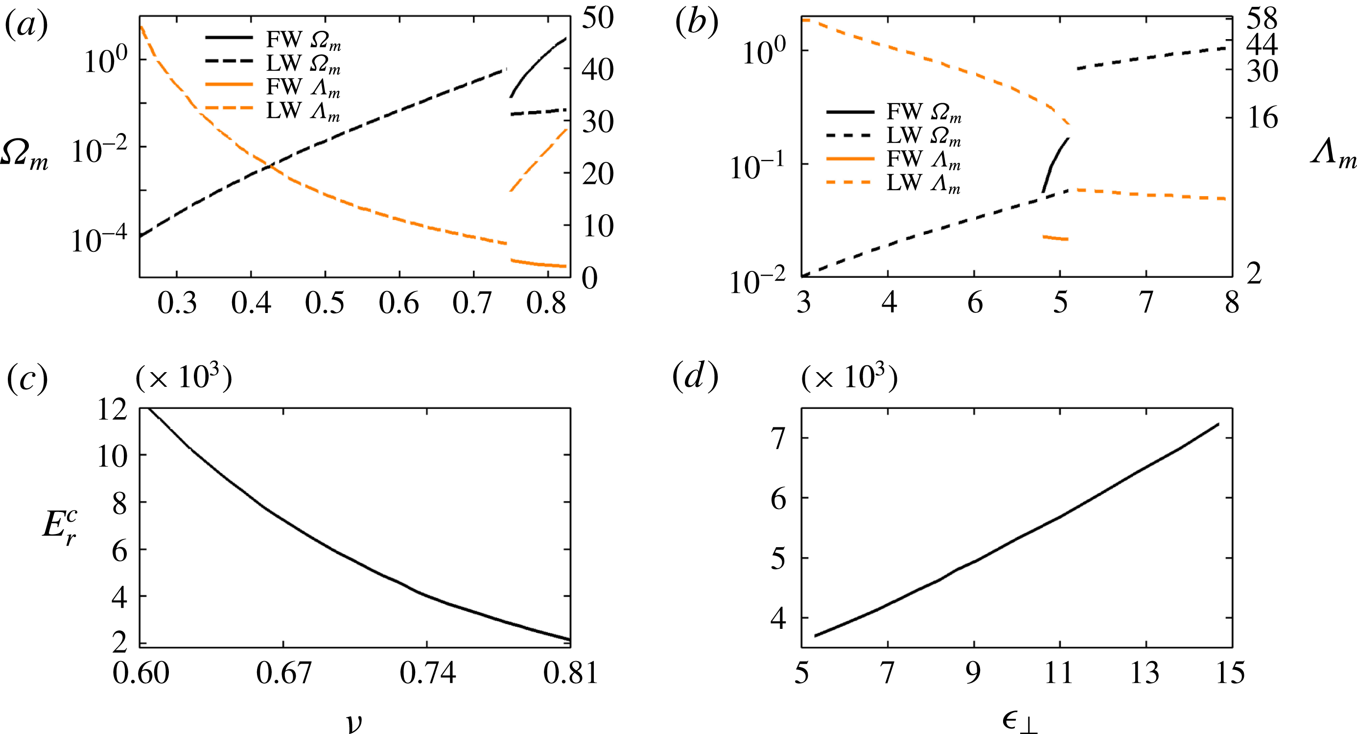
Panels (a,b) show the sole existence of the LW mode (broken line) at lower values of
 $\unicode[STIX]{x1D708}$
and
 $\unicode[STIX]{x1D716}_{\bot }$
when the orientations of all the molecules across the film are planar
 $(\unicode[STIX]{x1D703}_{,Z}=0)$
. However, at higher values of
 $\unicode[STIX]{x1D708}$
and
 $\unicode[STIX]{x1D716}_{\bot }$
, the FTT stimulates the appearance of the FW mode (solid line) of instability alongside the LW mode. The broken lines in panel (a) suggest that the dominant time scales corresponding to the LW mode progressively reduce with the variation in
 $\unicode[STIX]{x1D708}$
before the FTT takes place. The solid lines show that both the time and the length scales of the FW mode of instability reduce with increasing
 $\unicode[STIX]{x1D708}$
. After the FTT, the FW mode dominates over the LW mode. The broken lines in panel (b) show that with the enhancement of
 $\unicode[STIX]{x1D716}_{\bot }$
the LW mode of the EHD instability largely dominates over the FW mode before and after the FTT. However, near the transition, the FW mode becomes dominant for a very small range of
 $\unicode[STIX]{x1D716}_{\bot }$
. Panels (c,d) summarize the variation in the critical
 $E_{r}(E_{r}^{c})$
for the FTT with
 $\unicode[STIX]{x1D708}$
and
 $\unicode[STIX]{x1D716}_{\bot }$
. These plots suggest that a higher EHD stress at higher values of
 $\unicode[STIX]{x1D708}$
can cause the FTT at a much smaller value of
 $E_{r}^{c}$
, whereas enhancement of
 $\unicode[STIX]{x1D716}_{\bot }$
may increase the
 $E_{r}^{c}$
required for the FTT owing to the induced charge separation normal to the electric field after the rotation of the nematic axis due to the FTT. Concisely, figures 10 and 11 together show the influence of various thermodynamic parameters such as applied voltage, Ericksen stress, film thickness, and dielectric anisotropy of the materials on the possible modes of instability, and subsequently on the FTT.
Thus far, we considered only strong anchoring boundary conditions at the NS and NI interfaces. However, the NLC molecules can also show weak anchoring (Raghunathan Reference Raghunathan1995; Barbero, Evangelista & Madhusudana Reference Barbero, Evangelista and Madhusudana1998; Guan & Yang Reference Guan and Yang2003; Otten & van der Schoot Reference Otten and van der Schoot2009; Zhang, Zhang, Zhu & Xuan Reference Zhang, Zhang, Zhu and Xuan2011), especially near the NI interface. This effect can be incorporated in the GLSA using the Rapini–Papoular surface energy density as the weak anchoring energy, which can be written as
 $F_{s}=(1/2)\unicode[STIX]{x1D70F}_{0}[1+\unicode[STIX]{x1D714}(\boldsymbol{n}\boldsymbol{\cdot }\boldsymbol{n}_{s})^{2}]$
, where the anchoring strength of the director at the free surface is defined as
 $w_{p}=\unicode[STIX]{x1D70F}_{0}\unicode[STIX]{x1D714}$
(Rapini & Papoular Reference Rapini and Papoular1969; Cummings Reference Cummings2004; Stewart Reference Stewart2004). Consequently, the boundary condition at the NI interface
 $(z=h)$
(2.16) is replaced by (Jenkins & Barratt Reference Jenkins and Barratt1974)
 $$\begin{eqnarray}\unicode[STIX]{x1D70E}\boldsymbol{n}-(\unicode[STIX]{x2202}F/\unicode[STIX]{x2202}\unicode[STIX]{x1D735}\boldsymbol{n})\boldsymbol{\cdot }\boldsymbol{n}_{s}-\unicode[STIX]{x2202}F_{s}/\unicode[STIX]{x2202}\boldsymbol{n}=0,\end{eqnarray}$$
where
 $\unicode[STIX]{x1D70E}$
is an arbitrary scalar. Eliminating the scalar term from the
 $X$
- and
 $Z$
-components of the (7.5), the following free surface weak anchoring boundary condition at the NI interface
 $(Z=H)$
is obtained
 $$\begin{eqnarray}\unicode[STIX]{x1D703}_{,Z}+\unicode[STIX]{x1D6FF}_{1}K_{24}\sin 2\unicode[STIX]{x1D703}\hspace{2.22198pt}\unicode[STIX]{x1D703}_{,X}-\unicode[STIX]{x1D6FF}_{1}^{2}\unicode[STIX]{x1D703}_{,X}H_{,X}-E_{r}W_{p}(2\unicode[STIX]{x1D6FF}_{1}\cos 2\unicode[STIX]{x1D703}H_{,X}+\sin 2\unicode[STIX]{x1D703}(1-\unicode[STIX]{x1D6FF}_{1}^{2}H_{,X}^{2}))=0,\end{eqnarray}$$
Here, the dimensionless parameter
 $W_{p}=w_{p}h_{0}/\unicode[STIX]{x1D716}_{0}\unicode[STIX]{x1D713}_{0}^{2}$
signifies the ratio of the anchoring force at the interface to the force applied by the electric field. The notation
 $K_{24}(=k_{24}/K_{f})$
represents one of the non-dimensional saddle-splay elastic constants. Equation (7.6) has been used in place of (3.17) during the weak anchoring analysis, which is perturbed by employing the normal linear modes shown in § 4 to obtain the following base- and perturbed-state conditions at
 $Z=\bar{H}$
and
 $Z=H$
 $$\begin{eqnarray}\displaystyle & \displaystyle \bar{\unicode[STIX]{x1D703}}_{,Z}-E_{r}W_{p}\sin 2\bar{\unicode[STIX]{x1D703}}=0, & \displaystyle\end{eqnarray}$$
 $$\begin{eqnarray}\displaystyle & \displaystyle 2\text{i}K\unicode[STIX]{x1D6FF}_{1}E_{r}W_{p}\cos 2\bar{\unicode[STIX]{x1D703}}\tilde{W}-\unicode[STIX]{x1D6FA}\tilde{\unicode[STIX]{x1D703}}_{,Z}-\unicode[STIX]{x1D6FA}(\text{i}K\unicode[STIX]{x1D6FF}_{1}K_{24}\sin 2\bar{\unicode[STIX]{x1D703}}-2E_{r}W_{p}\cos 2\bar{\unicode[STIX]{x1D703}})\tilde{\unicode[STIX]{x1D703}}=0. & \displaystyle\end{eqnarray}$$
Equations (7.7) and (7.8) are employed in place of (4.7b
) and (4.18) for the weak anchoring analysis. While performing the numerical analysis, as shown in § 5, (7.8) has been transformed into the
 $\unicode[STIX]{x1D709}$
and
 $\unicode[STIX]{x1D712}$
space at the NI interface (
 $\unicode[STIX]{x1D709}=1$
and
 $\unicode[STIX]{x1D712}=1$
) as
 $$\begin{eqnarray}2\text{i}K\unicode[STIX]{x1D6FF}_{1}E_{r}W_{p}\cos 2\bar{\unicode[STIX]{x1D703}}\tilde{W}-2\unicode[STIX]{x1D6FA}\tilde{\unicode[STIX]{x1D703}}_{,\unicode[STIX]{x1D709}}-\unicode[STIX]{x1D6FA}(\text{i}K\unicode[STIX]{x1D6FF}_{1}K_{24}\sin 2\bar{\unicode[STIX]{x1D703}}-2E_{r}W_{p}\cos 2\bar{\unicode[STIX]{x1D703}})\tilde{\unicode[STIX]{x1D703}}=0.\end{eqnarray}$$
Equation (7.9) has been employed for the weak anchoring analysis instead of (5.8), which was previously employed to perform the strong anchoring case at the NI interface. It may also be noted here that, in this formulation, the saddle-splay term,
 $K_{24}$
, is considered. Barring these modifications, all the other governing equations and the boundary conditions are kept unchanged while weak anchoring analysis is carried out. The set of governing equations and boundary conditions for the weak anchoring analysis suggest that the higher to lower values of the parameter
 $w_{p}$
indicate weak to strong anchoring conditions at the NI interface. Figure 12 shows results from the GLSA with the P–W orientation at the interfaces, which means strong planar anchoring (P) at the NS interface and weak anchoring (W) at the NI interface. Curves 1 and 2 in panel (a) also show the variations in the base-state orientations of the NLC molecules, while the schematic diagrams S1 and S2 show the orientations of the molecules across the NLC film before and after the FTT. Panels (b,c) show the existence of an LW mode at
 $E_{r}=41.5$
for
 $\unicode[STIX]{x1D703}_{,Z}=0$
, whereas at
 $E_{r}=43$
there is a rapid change in
 $\unicode[STIX]{x1D6FA}$
with variations in the orientation of the molecules across the film due to FTT. The abrupt changeover of the director orientation across the film with increasing
 $E_{r}$
is also indicated by the discontinuities in panel (c).
GLSA results of an NLC film with P–W orientations (
 $\unicode[STIX]{x1D703}_{1}=90^{\circ }$
and
 $\unicode[STIX]{x1D703}_{2}=W$
) at the NS and NI boundaries. (a) Curves 1 (blue) and 2 (olive) show the variation of
 $\bar{\unicode[STIX]{x1D703}}$
along the
 $Z$
-axis at
 $E_{r}=41.5$
and 43.0, respectively, which is also schematically shown by the diagrams S1 and S2. (b) Curves 1 (blue) and 2 (olive) show the variation of
 $\unicode[STIX]{x1D6FA}$
with
 $K$
corresponding to panel (a). The parameters,
 $w_{p}=2\times 10^{-7}~\text{N}~\text{m}^{-1}$
(McGinn et al.
Reference Mcginn, Laderman, Zimmermann, Kitzerow and Collings2013),
 $K_{f}=3$
pN, and
 $k_{24}=0.6$
pN are kept constant in these plots. (c,d) Variations of
 $\unicode[STIX]{x1D6FA}_{m}$
and
 $\unicode[STIX]{x1D6EC}_{m}$
with
 $E_{r}$
. The
 $w_{p}$
values used for these plots are
 $2\times 10^{-7}~\text{N}~\text{m}^{-1}$
and
 $2\times 10^{-10}~\text{N}~\text{m}^{-1}$
. The circular and square symbols in panel (d) correspond to the strong anchoring condition, P–P. The other necessary parameters for the plots are shown in table 1.

As compared to the results shown in the figure 10 for the strong anchoring P–P boundary conditions at the interfaces, enforcing the P–W boundary condition at the NS and NI interfaces leads to the following changes: (i) only the LW mode is observed while the finite-wavenumber instability is absent even after the FTT (figure 12
b); (ii) after the FTT, the director orientation across the bulk and at the NI interface align towards the electric field (diagram S2); (iii) the magnitude of
 $\unicode[STIX]{x1D703}_{,Z}$
near the NI interface becomes negligible owing to the movement of the boundary as well as bulk molecules towards the electric field due to the weak anchoring condition, which reduces the magnitude of the Ericksen stress to suppress the inception of the FW mode; (iv) the FTT happens at a much lower value of
 $E_{r}=43$
(panels b and c). When the other parameters are kept similar, the voltage necessary for the transition is approximately 5.4 V for the P–W case as compared to 50 V for the P–P case. Interestingly, while at the higher values of
 $w_{p}$
we observe all the aforementioned attributes related to the P–W case, the same system can asymptotically reproduce the results related to the P–P case (symbols, panel d) having strong anchoring boundary conditions at smaller values of
 $w_{p}$
(solid line, panel d). In brief, figure 12 shows some of the salient features of the EHD instabilities of NLC films and FTT when a weak anchoring boundary condition is enforced at the NI interface.
7.5 Analysis for wave vector perpendicular to director orientation
Owing to the 2-D nature of the present GLSA formalism, the wave vector is always restricted in the direction of the director orientation during the free surface deformation. In one of the seminal contributions, Raghunathan (Reference Raghunathan1995) showed a methodology in which the influence of the director orientation perpendicular to the wave vector can be theoretically analysed under a 2-D framework. The formulation of Raghunathan (Reference Raghunathan1995) can be extended to the proposed GLSA in the following manner: (i) the governing equations and the boundary conditions in the
 $y$
- and
 $z$
-directions are considered and made dimensionless following the procedure mentioned in § 3.1; (ii) the base-state governing equations and boundary conditions are considered in the
 $x$
- and
 $z$
-directions following the methodology mentioned in § 4.1; (iii) the dimensionless governing equations and boundary conditions are linearized employing the normal linear modes,
 $\hat{V}=\tilde{V}(Z)\exp [\unicode[STIX]{x1D6FA}T+\text{i}K_{Y}Y]$
,
 ${\hat{W}}=\tilde{W}(Z)\exp [\unicode[STIX]{x1D6FA}T+\text{i}K_{Y}Y]$
,
 $\hat{P}=\bar{P}+\tilde{P}(Z)\exp [\unicode[STIX]{x1D6FA}T+\text{i}K_{Y}Y]$
,
 $[\unicode[STIX]{x1D6F9},\unicode[STIX]{x1D6F9}_{a}]=[\bar{\unicode[STIX]{x1D6F9}}(Z),\bar{\unicode[STIX]{x1D6F9}_{a}}(Z)]+[\tilde{\unicode[STIX]{x1D6F9}}(Z),\tilde{\unicode[STIX]{x1D6F9}_{a}}(Z)]\exp [\unicode[STIX]{x1D6FA}T+\text{i}K_{Y}Y]$
,
 $H=\bar{H}+\tilde{H}(Z)\exp [\unicode[STIX]{x1D6FA}T+\text{i}K_{Y}Y]$
,
 $\unicode[STIX]{x1D703}=\bar{\unicode[STIX]{x1D703}}(Z)+\tilde{\unicode[STIX]{x1D703}}(Z)\exp [\unicode[STIX]{x1D6FA}T+\text{i}K_{Y}Y]$
, and
 $\unicode[STIX]{x1D719}=\tilde{\unicode[STIX]{x1D719}}(Z)\exp [\unicode[STIX]{x1D6FA}T+\text{i}K_{Y}Y]$
, where
 $K_{Y}$
is the wavenumber of perturbations in the
 $Y$
-direction and
 $\unicode[STIX]{x1D719}$
is the azimuthal angle of the director orientation. The linearized governing equations and boundary conditions for this analysis are shown in appendix D; (iv) the set of ODEs are numerically solved by employing the same procedure discussed in § 5.
GLSA results with the perturbation of the wave vector along the
 $y$
-direction with both the P–P (
 $\unicode[STIX]{x1D703}_{1}=90^{\circ }$
and
 $\unicode[STIX]{x1D703}_{2}=90^{\circ }$
) (a–c) and the H–H (
 $\unicode[STIX]{x1D703}_{1}=0^{\circ }$
and
 $\unicode[STIX]{x1D703}_{2}=0^{\circ }$
) (d–f) orientations at the NS and NI boundaries when
 $\unicode[STIX]{x1D716}_{d}=9$
and
 $\unicode[STIX]{x1D708}=0.75$
. (a) Curves 1 (blue) and 2 (olive) show the variation of
 $\bar{\unicode[STIX]{x1D703}}$
along the
 $Z$
-axis at
 $E_{r}=3543.1$
and 3689.2, respectively, which is also schematically shown by the diagrams S1 and S2. (b) Curves 1 (blue) and 2 (olive) show the variation of
 $\unicode[STIX]{x1D6FA}$
with
 $K$
corresponding to panel (a). (d) Variation of director orientation at the base state
 $(\bar{\unicode[STIX]{x1D703}})$
along the
 $Z$
-axis as schematically also shown in the diagram S1. (e)
 $\unicode[STIX]{x1D6FA}$
versus
 $K$
curves for this case where curves 1–5 represent
 $E_{r}=354.2$
, 796.9, 1416.6, 2213.5, and 3187.4, respectively. (c,f) Variations of
 $\unicode[STIX]{x1D6FA}_{m}$
and
 $\unicode[STIX]{x1D6EC}_{m}$
with
 $E_{r}$
. Other parameters used for these plots are shown in table 1.

Figure 13 shows the results obtained from this analysis, which are compared and contrasted with the results previously shown in figures 6 and 10. Panels (a–c) suggest that for the case with P–P orientations at the NI and NS interfaces, the
 $E_{r}^{c}$
for FTT remain exactly same as was previously predicted in figure 10(d). In addition, the regime for
 $\unicode[STIX]{x1D6EC}_{m}$
also remains the same in figures 10(d) and 13(c). Crucially, the values of
 $\unicode[STIX]{x1D6FA}$
and
 $\unicode[STIX]{x1D6FA}_{m}$
are found to be marginally higher in the present case than the one shown in figures 10(b) and 10(d), which indicates that at the perturbed state the director orientation is perhaps more favourable in the
 $y$
-direction than in the
 $x$
-direction, when the base state of the system is in the
 $x$
–
 $z$
plane. However, relatively higher values of
 $\unicode[STIX]{x1D6FA}$
and
 $\unicode[STIX]{x1D6FA}_{m}$
in the present case can also be attributed to the absence of the azimuthal base state
 $(\bar{\unicode[STIX]{x1D719}})$
, which provides a more (less) facile director orientation in the perturbed state towards the normal (parallel) direction of the base state. Further, the magnitudes of
 $\unicode[STIX]{x1D6FA}$
and
 $\unicode[STIX]{x1D6FA}_{m}$
shown in panels (d–f) suggest that even in the absence of the FTT, for the EHD instabilities, the director orientation at the perturbed state is more favourable in the
 $y$
-direction than in the
 $x$
-direction. However, again, for the EHD modes the regime for
 $\unicode[STIX]{x1D6EC}_{m}$
remain same in figures 6(c) and 13(f). It is important to note here that, in the present analysis, perhaps the absence of the azimuthal base state
 $(\bar{\unicode[STIX]{x1D719}})$
has made the director orientation in the perturbed state energetically more favourable in the normal direction to the base state. These occurrences can only be conclusively established when a comprehensive 3-D analysis with base-state polar and azimuthal director orientations
 $(\bar{\unicode[STIX]{x1D703}}\text{ and }\bar{\unicode[STIX]{x1D719}})$
is performed on the present system, which we keep as a future scope of research work.
8 Conclusions
The different modes of the electric field induced free surface instabilities of a thin nematic film have been explored through a comprehensive linear stability analysis. The Ericksen–Leslie governing equations for the dynamics of the nematic film together with the Maxwell stresses for the anisotropic electric field are linearized with appropriate boundary conditions to identify the time and the length scales. The major conclusions are:
(i) The study emphasizes the importance of general linear stability analysis over the most widely employed long-wave analysis to uncover the diverse stability paradigms of thin nematic films. In particular, the reported results suggest that thermodynamic parameters such as the dielectric anisotropy of the film, strength of external electric field, Frank elasticity, and Ericksen elastic stress play crucial roles in changing the time and length scales of the electric-field-induced instabilities of nematic films, while kinetic parameters such as the Leslie viscosity coefficients can only influence the time scale of the same.
(ii) The study reveals the presence of a pair of instability modes for the free surface instabilities of nematic films under an electric field. The long-wave interfacial mode is dominant when the sole destabilizing influence of the electric field subdues the Frank elasticity and surface tension. The finite-wavenumber mode is stimulated by the combined destabilizing influences originating from the anisotropic electric field and Ericksen stress for the films with positive dielectric anisotropy and weaker Frank elasticity.
(iii) A nematic film with positive dielectric anisotropy can show a bimodal instability with a long-wave interfacial mode and a shorter-wavelength finite-wavenumber mode when the combined effects of the Ericksen and electrohydrodynamic stresses subdue to Frank bulk elasticity and the surface tension forces. The long-wave mode is found to be the dominant mode in the bimodal instability at lower electric field strength or for films with larger Frank bulk elasticity. In contrast, the finite-wavenumber mode is found to be the dominant mode at higher field electric intensities where the Ericksen stress is significantly high. In comparison, the films with negative dielectric anisotropy show the long-wave interfacial mode of instability.
(iv) A FTT is observed for the films with positive dielectric anisotropy with a base-state planar–planar arrangement at the boundaries. The transition is associated with the change in the director orientations across the film as well as the induced charge separation along the direction of the field with increasing field intensity. The transition is also associated with a changeover of the instability from unimodal to bimodal because, at higher field intensities, the variation in the director orientations across the film helps in fuelling up the finite-wavenumber mode alongside the long-wave interfacial mode.
(v) Strong to weak anchoring conditions at the NI interface are found to have significant influence on the onset conditions of the FTT as well as on the modes of the electric field induced instabilities of the nematic liquid crystal film. Further, an analysis on the possibility of an unstable wave vector in the perturbed state normal to the director orientation in the base state showed that although the predictions associated with the electrohydrodynamic instabilities and FTT remain nearly similar, the director orientation at the perturbed state can be energetically more (less) favourable in the normal (parallel) direction of the base state. This occurrence can be attributed to the absence of the azimuthal base state in the formulation shown. A more comprehensive 3-D analysis in the presence of the base-state polar and azimuthal director orientations may usher in more clarity on this aspect, which is perhaps beyond the scope of the present work.
Concisely, the study uncovers a number of intriguing aspects of the free surface instabilities of thin nematic films under the influence of an external electric field, which has not been explored so far. As a future scope of work, apart from 3-D analysis with the consideration of a generic director orientation, the proposed theoretical model can be extended to systems having defects on the free surface or at the substrate–film interface (Berreman Reference Berreman1972; Fukuda, Yoneya & Yokoyama Reference Fukuda, Yoneya and Yokoyama2007).
Acknowledgements
We thank DeitY grant no. 5(9)/2012-NANO, DST Fast Track grant no. SR/FTP/ETA-091/2009, and DST FIST-grant no. SR/FST/ETII-028/2010, Government of India, for financial supports.
Appendix A. Expressions of the complicated variables
The variables
 $A_{i}$
,
 $B_{i}$
,
 $C_{i}$
, and
 $D_{i}$
, in the dimensionless equations of motions (3.2) and (3.3) are
 $$\begin{eqnarray}\displaystyle & \displaystyle A_{1}=(\hat{\unicode[STIX]{x1D6FC}}_{1}\sin ^{4}\unicode[STIX]{x1D703}+\hat{\unicode[STIX]{x1D6FC}}_{4}+(\hat{\unicode[STIX]{x1D6FC}}_{5}+\hat{\unicode[STIX]{x1D6FC}}_{6})\sin ^{2}\unicode[STIX]{x1D703}), & \displaystyle\end{eqnarray}$$
 $$\begin{eqnarray}\displaystyle & \displaystyle A_{2}=\sin 2\unicode[STIX]{x1D703}(2\hat{\unicode[STIX]{x1D6FC}_{1}}\sin ^{2}\unicode[STIX]{x1D703}-\hat{\unicode[STIX]{x1D6FC}}_{2}-\hat{\unicode[STIX]{x1D6FC}}_{3}+\hat{\unicode[STIX]{x1D6FC}}_{5}+\hat{\unicode[STIX]{x1D6FC}}_{6})/4, & \displaystyle\end{eqnarray}$$
 $$\begin{eqnarray}\displaystyle & \displaystyle A_{3}=\sin 2\unicode[STIX]{x1D703}(2\hat{\unicode[STIX]{x1D6FC}_{1}}\sin ^{2}\unicode[STIX]{x1D703}+\hat{\unicode[STIX]{x1D6FC}}_{2}+\hat{\unicode[STIX]{x1D6FC}}_{3}+\hat{\unicode[STIX]{x1D6FC}}_{5}+\hat{\unicode[STIX]{x1D6FC}}_{6})/4, & \displaystyle\end{eqnarray}$$
 $$\begin{eqnarray}\displaystyle & \displaystyle A_{4}=\hat{\unicode[STIX]{x1D6FC}}_{1}\sin ^{2}2\unicode[STIX]{x1D703}/4; & \displaystyle\end{eqnarray}$$
 $$\begin{eqnarray}\displaystyle & \displaystyle B_{1}=\sin 2\unicode[STIX]{x1D703}(\hat{\unicode[STIX]{x1D6FC}}_{1}\sin ^{2}\unicode[STIX]{x1D703}+\hat{\unicode[STIX]{x1D6FC}}_{5})/2, & \displaystyle\end{eqnarray}$$
 $$\begin{eqnarray}\displaystyle & \displaystyle B_{2}=((\hat{\unicode[STIX]{x1D6FC}}_{1}\sin ^{2}2\unicode[STIX]{x1D703}/2)+(\hat{\unicode[STIX]{x1D6FC}}_{5}-\hat{\unicode[STIX]{x1D6FC}}_{2})\cos ^{2}\unicode[STIX]{x1D703}+(\hat{\unicode[STIX]{x1D6FC}}_{3}+\hat{\unicode[STIX]{x1D6FC}}_{6})\sin ^{2}\unicode[STIX]{x1D703}+\hat{\unicode[STIX]{x1D6FC}}_{4})/2, & \displaystyle\end{eqnarray}$$
 $$\begin{eqnarray}\displaystyle & \displaystyle B_{3}=((\hat{\unicode[STIX]{x1D6FC}}_{1}\sin ^{2}2\unicode[STIX]{x1D703}/2)+(\hat{\unicode[STIX]{x1D6FC}}_{2}+\hat{\unicode[STIX]{x1D6FC}}_{5})\cos ^{2}\unicode[STIX]{x1D703}+(\hat{\unicode[STIX]{x1D6FC}}_{6}-\hat{\unicode[STIX]{x1D6FC}}_{3})\sin ^{2}\unicode[STIX]{x1D703}+\hat{\unicode[STIX]{x1D6FC}}_{4})/2, & \displaystyle\end{eqnarray}$$
 $$\begin{eqnarray}\displaystyle & \displaystyle B_{4}=\sin 2\unicode[STIX]{x1D703}(\hat{\unicode[STIX]{x1D6FC}}_{1}\cos ^{2}\unicode[STIX]{x1D703}+\hat{\unicode[STIX]{x1D6FC}}_{6})/2; & \displaystyle\end{eqnarray}$$
 $$\begin{eqnarray}\displaystyle & \displaystyle C_{1}=\sin 2\unicode[STIX]{x1D703}(\hat{\unicode[STIX]{x1D6FC}}_{1}\sin ^{2}\unicode[STIX]{x1D703}+\hat{\unicode[STIX]{x1D6FC}}_{6})/2, & \displaystyle\end{eqnarray}$$
 $$\begin{eqnarray}\displaystyle & \displaystyle C_{2}=((\hat{\unicode[STIX]{x1D6FC}}_{1}\sin ^{2}2\unicode[STIX]{x1D703}/2)+(\hat{\unicode[STIX]{x1D6FC}}_{2}+\hat{\unicode[STIX]{x1D6FC}}_{5})\sin ^{2}\unicode[STIX]{x1D703}+(\hat{\unicode[STIX]{x1D6FC}}_{6}-\hat{\unicode[STIX]{x1D6FC}}_{3})\cos ^{2}\unicode[STIX]{x1D703}+\hat{\unicode[STIX]{x1D6FC}}_{4})/2, & \displaystyle\end{eqnarray}$$
 $$\begin{eqnarray}\displaystyle & \displaystyle C_{3}=((\hat{\unicode[STIX]{x1D6FC}}_{1}\sin ^{2}2\unicode[STIX]{x1D703}/2)+(\hat{\unicode[STIX]{x1D6FC}}_{5}-\hat{\unicode[STIX]{x1D6FC}}_{2})\sin ^{2}\unicode[STIX]{x1D703}+(\hat{\unicode[STIX]{x1D6FC}}_{6}+\hat{\unicode[STIX]{x1D6FC}}_{3})\cos ^{2}\unicode[STIX]{x1D703}+\hat{\unicode[STIX]{x1D6FC}}_{4})/2, & \displaystyle\end{eqnarray}$$
 $$\begin{eqnarray}\displaystyle & \displaystyle C_{4}=\sin 2\unicode[STIX]{x1D703}(\hat{\unicode[STIX]{x1D6FC}}_{1}\cos ^{2}\unicode[STIX]{x1D703}+\hat{\unicode[STIX]{x1D6FC}}_{5})/2; & \displaystyle\end{eqnarray}$$
 $$\begin{eqnarray}\displaystyle & \displaystyle D_{1}=\hat{\unicode[STIX]{x1D6FC}}_{1}\sin ^{2}2\unicode[STIX]{x1D703}/4, & \displaystyle\end{eqnarray}$$
 $$\begin{eqnarray}\displaystyle & \displaystyle D_{2}=\sin 2\unicode[STIX]{x1D703}(2\hat{\unicode[STIX]{x1D6FC}_{1}}\cos ^{2}\unicode[STIX]{x1D703}+\hat{\unicode[STIX]{x1D6FC}}_{2}+\hat{\unicode[STIX]{x1D6FC}}_{3}+\hat{\unicode[STIX]{x1D6FC}}_{5}+\hat{\unicode[STIX]{x1D6FC}}_{6})/4, & \displaystyle\end{eqnarray}$$
 $$\begin{eqnarray}\displaystyle & \displaystyle D_{3}=\sin 2\unicode[STIX]{x1D703}(2\hat{\unicode[STIX]{x1D6FC}_{1}}\cos ^{2}\unicode[STIX]{x1D703}-\hat{\unicode[STIX]{x1D6FC}}_{2}-\hat{\unicode[STIX]{x1D6FC}}_{3}+\hat{\unicode[STIX]{x1D6FC}}_{5}+\hat{\unicode[STIX]{x1D6FC}}_{6})/4, & \displaystyle\end{eqnarray}$$
 $$\begin{eqnarray}\displaystyle & \displaystyle D_{4}=(\hat{\unicode[STIX]{x1D6FC}}_{1}\cos ^{4}\unicode[STIX]{x1D703}+\hat{\unicode[STIX]{x1D6FC}}_{4}+(\hat{\unicode[STIX]{x1D6FC}}_{5}+\hat{\unicode[STIX]{x1D6FC}}_{6})\cos ^{2}\unicode[STIX]{x1D703}). & \displaystyle\end{eqnarray}$$
In the above expressions the dimensionless variables
 $\hat{\unicode[STIX]{x1D6FC}}_{i}=2\unicode[STIX]{x1D6FC}_{i}/\unicode[STIX]{x1D6FC}_{4}$
.
The expressions for the variables
 $L_{i}^{X}$
,
 $L_{i}^{Z}$
, and
 $L_{i}$
in the linearized equations (4.9)–(4.11) are provided as follows,
 $$\begin{eqnarray}\displaystyle & \displaystyle L_{1}^{X}=\bar{B}_{2}, & \displaystyle\end{eqnarray}$$
 $$\begin{eqnarray}\displaystyle & \displaystyle L_{2}^{X}=\text{i}K\unicode[STIX]{x1D6FF}_{1}(\bar{A}_{2}+\bar{B}_{1}-\bar{B}_{4})+\bar{B}_{2,Z}, & \displaystyle\end{eqnarray}$$
 $$\begin{eqnarray}\displaystyle & \displaystyle L_{3}^{X}=-K^{2}\unicode[STIX]{x1D6FF}_{1}^{2}(\bar{A}_{1}-\bar{A}_{4}-\bar{B}_{3})+\text{i}K\unicode[STIX]{x1D6FF}_{1}(\bar{B}_{1}-\bar{B}_{4})_{,Z}, & \displaystyle\end{eqnarray}$$
 $$\begin{eqnarray}\displaystyle & \displaystyle L_{4}^{X}=\text{i}K^{3}\unicode[STIX]{x1D6FF}_{1}^{3}\bar{A}_{3}+\unicode[STIX]{x1D6FF}_{1}^{2}K^{2}\bar{B}_{3,Z}, & \displaystyle\end{eqnarray}$$
 $$\begin{eqnarray}\displaystyle & \displaystyle L_{5}^{X}=-K^{2}E_{r}^{-1}\bar{\unicode[STIX]{x1D703}}_{,Z}; & \displaystyle\end{eqnarray}$$
 $$\begin{eqnarray}\displaystyle & \displaystyle L_{1}^{Z}=\unicode[STIX]{x1D6FF}_{1}\bar{D}_{2}, & \displaystyle\end{eqnarray}$$
 $$\begin{eqnarray}\displaystyle & \displaystyle L_{2}^{Z}=\text{i}K\unicode[STIX]{x1D6FF}_{1}^{2}(\bar{C}_{2}+\bar{D}_{1}-\bar{D}_{4})+\unicode[STIX]{x1D6FF}_{1}\bar{D}_{2,Z}, & \displaystyle\end{eqnarray}$$
 $$\begin{eqnarray}\displaystyle & \displaystyle L_{3}^{Z}=-K^{2}\unicode[STIX]{x1D6FF}_{1}^{3}(\bar{C}_{1}-\bar{C}_{4}-\bar{D}_{3})+\text{i}K\unicode[STIX]{x1D6FF}_{1}^{2}(\bar{D}_{1}-\bar{D}_{4})_{,Z}, & \displaystyle\end{eqnarray}$$
 $$\begin{eqnarray}\displaystyle & \displaystyle L_{4}^{Z}=\text{i}K^{3}\unicode[STIX]{x1D6FF}_{1}^{4}\bar{C}_{3}+K^{2}\unicode[STIX]{x1D6FF}_{1}^{3}\bar{D}_{3,Z}, & \displaystyle\end{eqnarray}$$
 $$\begin{eqnarray}\displaystyle & \displaystyle L_{5}^{Z}=2\text{i}KE_{r}^{-1}\bar{\unicode[STIX]{x1D703}}_{,Z}, & \displaystyle\end{eqnarray}$$
 $$\begin{eqnarray}\displaystyle & \displaystyle L_{6}^{Z}=\text{i}KE_{r}^{-1}\bar{\unicode[STIX]{x1D703}}_{,ZZ}, & \displaystyle\end{eqnarray}$$
 $$\begin{eqnarray}\displaystyle & \displaystyle L_{7}^{Z}=-\text{i}K^{3}\unicode[STIX]{x1D6FF}_{1}^{2}E_{r}^{-1}\bar{\unicode[STIX]{x1D703}}_{,Z}-2\text{i}K\unicode[STIX]{x1D716}_{d}\cos 2\bar{\unicode[STIX]{x1D703}}\hspace{2.22198pt}\bar{\unicode[STIX]{x1D703}}_{,Z}\bar{\unicode[STIX]{x1D6F9}}_{,Z}^{2}, & \displaystyle\end{eqnarray}$$
 $$\begin{eqnarray}\displaystyle & \displaystyle L_{8}^{Z}=-2\text{i}K\unicode[STIX]{x1D716}_{d}\sin 2\bar{\unicode[STIX]{x1D703}}\hspace{2.22198pt}\bar{\unicode[STIX]{x1D703}}_{,Z}\bar{\unicode[STIX]{x1D6F9}}_{,Z}, & \displaystyle\end{eqnarray}$$
 $$\begin{eqnarray}\displaystyle & \displaystyle L_{9}^{Z}=-2K^{2}\unicode[STIX]{x1D6FF}_{1}\unicode[STIX]{x1D716}_{d}\cos 2\bar{\unicode[STIX]{x1D703}}\hspace{2.22198pt}\bar{\unicode[STIX]{x1D703}}_{,Z}\bar{\unicode[STIX]{x1D6F9}}_{,Z}; & \displaystyle\end{eqnarray}$$
 $$\begin{eqnarray}\displaystyle & \displaystyle L_{1}=\bar{B}_{2}, & \displaystyle\end{eqnarray}$$
 $$\begin{eqnarray}\displaystyle & \displaystyle L_{2}=\text{i}K\unicode[STIX]{x1D6FF}_{1}(\bar{A}_{2}+\bar{B}_{1}-\bar{B}_{4}-\bar{D}_{2})+2\bar{B}_{2,Z}, & \displaystyle\end{eqnarray}$$
 $$\begin{eqnarray}\displaystyle & & \displaystyle L_{3}=-K^{2}\unicode[STIX]{x1D6FF}_{1}^{2}(\bar{A}_{1}-\bar{A}_{4}-\bar{B}_{3}-\bar{C}_{2}-\bar{D}_{1}+\bar{D}_{4})\nonumber\\ \displaystyle & & \displaystyle \quad +\,\text{i}K\unicode[STIX]{x1D6FF}_{1}(\bar{A}_{2}+2(\bar{B}_{1}-\bar{B}_{4})-\bar{D}_{2})_{,Z}+\bar{B}_{2,ZZ},\end{eqnarray}$$
 $$\begin{eqnarray}\displaystyle & L_{4}=\text{i}K^{3}\unicode[STIX]{x1D6FF}_{1}^{3}(\bar{A}_{3}+\bar{C}_{1}-\bar{C}_{4}-\bar{D}_{3})+\text{i}K\unicode[STIX]{x1D6FF}_{1}\bar{B}_{1,ZZ} & \displaystyle \nonumber\\ \displaystyle & -\text{i}K\unicode[STIX]{x1D6FF}_{1}\bar{B}_{4,ZZ}-K^{2}\unicode[STIX]{x1D6FF}_{1}^{2}(\bar{A}_{1}-\bar{A}_{4}-2\bar{B}_{3}-\bar{D}_{1}+\bar{D}_{4})_{,Z}, & \displaystyle\end{eqnarray}$$
 $$\begin{eqnarray}\displaystyle & \displaystyle L_{5}=K^{4}\unicode[STIX]{x1D6FF}_{1}^{4}\bar{C}_{3}+\text{i}K^{3}\unicode[STIX]{x1D6FF}_{1}^{3}(\bar{A}_{3}-\bar{D}_{3})_{,Z}+K^{2}\unicode[STIX]{x1D6FF}_{1}^{2}\bar{B}_{3,ZZ}, & \displaystyle\end{eqnarray}$$
 $$\begin{eqnarray}\displaystyle & \displaystyle L_{6}=K^{2}E_{r}^{-1}\bar{\unicode[STIX]{x1D703}}_{,Z}, & \displaystyle\end{eqnarray}$$
 $$\begin{eqnarray}\displaystyle & \displaystyle L_{7}=-K^{4}\unicode[STIX]{x1D6FF}_{1}^{2}E_{r}^{-1}\bar{\unicode[STIX]{x1D703}}_{,Z}-2K^{2}\unicode[STIX]{x1D716}_{d}\cos 2\bar{\unicode[STIX]{x1D703}}\hspace{2.22198pt}\bar{\unicode[STIX]{x1D703}}_{,Z}\bar{\unicode[STIX]{x1D6F9}}_{,Z}^{2}, & \displaystyle\end{eqnarray}$$
 $$\begin{eqnarray}\displaystyle & \displaystyle L_{8}=-2K^{2}\unicode[STIX]{x1D716}_{d}\sin 2\bar{\unicode[STIX]{x1D703}}\hspace{2.22198pt}\bar{\unicode[STIX]{x1D703}}_{,Z}\bar{\unicode[STIX]{x1D6F9}}_{,Z}, & \displaystyle\end{eqnarray}$$
 $$\begin{eqnarray}\displaystyle & \displaystyle L_{9}=2\text{i}K^{3}\unicode[STIX]{x1D6FF}_{1}\unicode[STIX]{x1D716}_{d}\cos 2\bar{\unicode[STIX]{x1D703}}\hspace{2.22198pt}\bar{\unicode[STIX]{x1D703}}_{,Z}\bar{\unicode[STIX]{x1D6F9}}_{,Z}. & \displaystyle\end{eqnarray}$$
The expressions for the variables
 $S_{i}^{N}$
and
 $S_{i}^{T}$
in the linearized equations (4.14) and (4.15) are provided as follows,
 $$\begin{eqnarray}\displaystyle & \displaystyle S_{1}^{N}=K^{4}-\text{i}K^{3}\unicode[STIX]{x1D6FF}_{1}\unicode[STIX]{x1D716}_{d}\sin 2\bar{\unicode[STIX]{x1D703}}\hspace{2.22198pt}\bar{\unicode[STIX]{x1D6F9}}_{,Z}^{2}, & \displaystyle\end{eqnarray}$$
 $$\begin{eqnarray}\displaystyle & \displaystyle S_{2}^{N}=-\bar{B}_{2}, & \displaystyle\end{eqnarray}$$
 $$\begin{eqnarray}\displaystyle & \displaystyle S_{3}^{N}=-\text{i}K\unicode[STIX]{x1D6FF}_{1}(\bar{A}_{1}+\bar{B}_{1}-\bar{B}_{4}-\bar{D}_{2})-\bar{B}_{2,Z}, & \displaystyle\end{eqnarray}$$
 $$\begin{eqnarray}\displaystyle & \displaystyle S_{4}^{N}=K^{2}\unicode[STIX]{x1D6FF}_{1}^{2}(\bar{A}_{1}-\bar{A}_{4}-\bar{B}_{3}-\bar{D}_{1}+\bar{D}_{4})-\text{i}K\unicode[STIX]{x1D6FF}_{1}(\bar{B}_{1}-\bar{B}_{4})_{,Z}, & \displaystyle\end{eqnarray}$$
 $$\begin{eqnarray}\displaystyle & \displaystyle S_{5}^{N}=-\text{i}K^{3}\unicode[STIX]{x1D6FF}_{1}^{3}(\bar{A}_{3}-\bar{D}_{3})-K^{2}\unicode[STIX]{x1D6FF}_{1}^{2}\bar{B}_{3,Z}, & \displaystyle\end{eqnarray}$$
 $$\begin{eqnarray}\displaystyle & \displaystyle S_{6}^{N}=-K^{2}E_{r}^{-1}\bar{\unicode[STIX]{x1D703}}_{,Z}, & \displaystyle\end{eqnarray}$$
 $$\begin{eqnarray}\displaystyle & \displaystyle S_{7}^{N}=-K^{2}\unicode[STIX]{x1D716}_{d}\sin 2\bar{\unicode[STIX]{x1D703}}\hspace{2.22198pt}\bar{\unicode[STIX]{x1D6F9}}_{,Z}^{2}, & \displaystyle\end{eqnarray}$$
 $$\begin{eqnarray}\displaystyle & \displaystyle S_{8}^{N}=2K^{2}(\unicode[STIX]{x1D716}_{\bot }+\unicode[STIX]{x1D716}_{d}\cos ^{2}\bar{\unicode[STIX]{x1D703}})\bar{\unicode[STIX]{x1D6F9}}_{,Z}, & \displaystyle\end{eqnarray}$$
 $$\begin{eqnarray}\displaystyle & \displaystyle S_{9}^{N}=-2K^{2}\bar{\unicode[STIX]{x1D6F9}}_{a,Z}; & \displaystyle\end{eqnarray}$$
 $$\begin{eqnarray}\displaystyle & \displaystyle S_{1}^{T}=K^{2}E_{r}^{-1}\bar{\unicode[STIX]{x1D703}}_{,Z}^{2}, & \displaystyle\end{eqnarray}$$
 $$\begin{eqnarray}\displaystyle & \displaystyle S_{2}^{T}=-\bar{B}_{2}, & \displaystyle\end{eqnarray}$$
 $$\begin{eqnarray}\displaystyle & \displaystyle S_{3}^{T}=-\text{i}K\unicode[STIX]{x1D6FF}_{1}(\bar{B}_{1}-\bar{B}_{4}), & \displaystyle\end{eqnarray}$$
 $$\begin{eqnarray}\displaystyle & \displaystyle S_{4}^{T}=-K^{2}\unicode[STIX]{x1D6FF}_{1}^{2}\bar{B}_{3}, & \displaystyle\end{eqnarray}$$
 $$\begin{eqnarray}\displaystyle & \displaystyle S_{5}^{T}=K^{2}E_{r}^{-1}\bar{\unicode[STIX]{x1D703}}_{,Z}. & \displaystyle\end{eqnarray}$$
The expressions for the variables
 $I_{i}$
in the linearized equation (4.16) are provided as follows,
 $$\begin{eqnarray}\displaystyle & \displaystyle I_{1}=\unicode[STIX]{x1D6FF}_{1}(\unicode[STIX]{x1D6EC}_{1}-\unicode[STIX]{x1D6EC}_{2}\cos 2\bar{\unicode[STIX]{x1D703}})/2, & \displaystyle\end{eqnarray}$$
 $$\begin{eqnarray}\displaystyle & \displaystyle I_{2}=-\text{i}K\unicode[STIX]{x1D6FF}_{1}^{2}\unicode[STIX]{x1D6EC}_{2}\sin 2\bar{\unicode[STIX]{x1D703}}, & \displaystyle\end{eqnarray}$$
 $$\begin{eqnarray}\displaystyle & \displaystyle I_{3}=-K^{2}\unicode[STIX]{x1D6FF}_{1}^{3}(\unicode[STIX]{x1D6EC}_{1}+\unicode[STIX]{x1D6EC}_{2}\cos 2\bar{\unicode[STIX]{x1D703}})/2, & \displaystyle\end{eqnarray}$$
 $$\begin{eqnarray}\displaystyle & \displaystyle I_{4}=-\text{i}KE_{r}^{-1}, & \displaystyle\end{eqnarray}$$
 $$\begin{eqnarray}\displaystyle & \displaystyle I_{5}=\text{i}K^{3}\unicode[STIX]{x1D6FF}_{1}^{2}E_{r}^{-1}+2\text{i}K\unicode[STIX]{x1D716}_{d}\cos 2\bar{\unicode[STIX]{x1D703}}\hspace{2.22198pt}\bar{\unicode[STIX]{x1D6F9}}_{,Z}^{2}, & \displaystyle\end{eqnarray}$$
 $$\begin{eqnarray}\displaystyle & \displaystyle I_{6}=2\text{i}K\unicode[STIX]{x1D716}_{d}\sin 2\bar{\unicode[STIX]{x1D703}}\hspace{2.22198pt}\bar{\unicode[STIX]{x1D6F9}}_{,Z}, & \displaystyle\end{eqnarray}$$
 $$\begin{eqnarray}\displaystyle & \displaystyle I_{7}=2K^{2}\unicode[STIX]{x1D6FF}_{1}\unicode[STIX]{x1D716}_{d}\cos 2\bar{\unicode[STIX]{x1D703}}\hspace{2.22198pt}\bar{\unicode[STIX]{x1D6F9}}_{,Z}. & \displaystyle\end{eqnarray}$$
The expressions for the variables
 $J_{i}$
in the linearized equations (4.19) and (4.20) are provided as follows,
 $$\begin{eqnarray}\displaystyle & \displaystyle J_{1}=\unicode[STIX]{x1D716}_{d}\sin 2\bar{\unicode[STIX]{x1D703}}\hspace{2.22198pt}\bar{\unicode[STIX]{x1D6F9}}_{,Z}, & \displaystyle\end{eqnarray}$$
 $$\begin{eqnarray}\displaystyle & \displaystyle J_{2}=\unicode[STIX]{x1D716}_{d}\sin 2\bar{\unicode[STIX]{x1D703}}\hspace{2.22198pt}\bar{\unicode[STIX]{x1D6F9}}_{,ZZ}+2\unicode[STIX]{x1D716}_{d}\cos 2\bar{\unicode[STIX]{x1D703}}\hspace{2.22198pt}\bar{\unicode[STIX]{x1D703}}_{,Z}\bar{\unicode[STIX]{x1D6F9}}_{,Z}-\text{i}K\unicode[STIX]{x1D6FF}_{1}\unicode[STIX]{x1D716}_{d}\cos 2\bar{\unicode[STIX]{x1D703}}\hspace{2.22198pt}\bar{\unicode[STIX]{x1D6F9}}_{,Z}, & \displaystyle\end{eqnarray}$$
 $$\begin{eqnarray}\displaystyle & \displaystyle J_{3}=-(\unicode[STIX]{x1D716}_{\bot }+\unicode[STIX]{x1D716}_{d}\cos ^{2}\bar{\unicode[STIX]{x1D703}}), & \displaystyle\end{eqnarray}$$
 $$\begin{eqnarray}\displaystyle & \displaystyle J_{4}=\unicode[STIX]{x1D716}_{d}\sin 2\bar{\unicode[STIX]{x1D703}}\hspace{2.22198pt}\bar{\unicode[STIX]{x1D703}}_{,Z}-\text{i}K\unicode[STIX]{x1D6FF}_{1}\unicode[STIX]{x1D716}_{d}\sin 2\bar{\unicode[STIX]{x1D703}}, & \displaystyle\end{eqnarray}$$
 $$\begin{eqnarray}\displaystyle & \displaystyle J_{5}=K^{2}\unicode[STIX]{x1D6FF}_{1}^{2}(\unicode[STIX]{x1D716}_{\bot }+\unicode[STIX]{x1D716}_{d}\sin ^{2}\bar{\unicode[STIX]{x1D703}})-\text{i}K\unicode[STIX]{x1D6FF}_{1}\unicode[STIX]{x1D716}_{d}\cos 2\bar{\unicode[STIX]{x1D703}}\hspace{2.22198pt}\bar{\unicode[STIX]{x1D703}}_{,Z}, & \displaystyle\end{eqnarray}$$
 $$\begin{eqnarray}\displaystyle & \displaystyle J_{6}=-K^{2}\unicode[STIX]{x1D6FF}_{1}^{2}. & \displaystyle\end{eqnarray}$$
The expressions for the variables
 $S_{i}^{E}$
in the linearized equation (4.22) are provided as follows,
 $$\begin{eqnarray}\displaystyle & \displaystyle S_{1}^{E}=\text{i}K\unicode[STIX]{x1D6FF}_{1}\unicode[STIX]{x1D716}_{d}\sin 2\bar{\unicode[STIX]{x1D703}}\hspace{2.22198pt}\bar{\unicode[STIX]{x1D6F9}}_{,Z}/2, & \displaystyle\end{eqnarray}$$
 $$\begin{eqnarray}\displaystyle & \displaystyle S_{2}^{E}=\unicode[STIX]{x1D716}_{d}\sin 2\bar{\unicode[STIX]{x1D703}}\hspace{2.22198pt}\bar{\unicode[STIX]{x1D6F9}}_{,Z}, & \displaystyle\end{eqnarray}$$
 $$\begin{eqnarray}\displaystyle & \displaystyle S_{3}^{E}=-(\unicode[STIX]{x1D716}_{\bot }+\unicode[STIX]{x1D716}_{d}\cos ^{2}\bar{\unicode[STIX]{x1D703}}), & \displaystyle\end{eqnarray}$$
 $$\begin{eqnarray}\displaystyle & \displaystyle S_{4}^{E}=-\text{i}K\unicode[STIX]{x1D6FF}_{1}\unicode[STIX]{x1D716}_{d}\sin 2\bar{\unicode[STIX]{x1D703}}/2. & \displaystyle\end{eqnarray}$$
The expressions for the variables
 $Q_{i}$
in the linearized equation (6.1) are provided as follows,
 $$\begin{eqnarray}\displaystyle & \displaystyle Q_{1}=2\unicode[STIX]{x1D6FF}_{1}^{2}(2+\hat{\unicode[STIX]{x1D6FC}}_{1}+\hat{\unicode[STIX]{x1D6FC}}_{3}+\hat{\unicode[STIX]{x1D6FC}}_{5})/(\hat{\unicode[STIX]{x1D6FC}}_{5}-\hat{\unicode[STIX]{x1D6FC}}_{2}+2), & \displaystyle\end{eqnarray}$$
 $$\begin{eqnarray}\displaystyle & \displaystyle Q_{2}=\unicode[STIX]{x1D6FF}_{1}^{4}(2+\hat{\unicode[STIX]{x1D6FC}}_{2}+2\hat{\unicode[STIX]{x1D6FC}}_{3}+\hat{\unicode[STIX]{x1D6FC}}_{5})/(\hat{\unicode[STIX]{x1D6FC}}_{5}-\hat{\unicode[STIX]{x1D6FC}}_{2}+2). & \displaystyle\end{eqnarray}$$
The expressions for the variables
 $\unicode[STIX]{x1D6FD}_{i}$
in the linearized equation (6.20) are provided as follows,
 $$\begin{eqnarray}\displaystyle & \displaystyle \unicode[STIX]{x1D6FD}_{1}=\sqrt{(Q_{1}-\sqrt{Q_{1}^{2}-4Q_{2}})/2}, & \displaystyle\end{eqnarray}$$
 $$\begin{eqnarray}\displaystyle & \displaystyle \unicode[STIX]{x1D6FD}_{2}=\sqrt{(Q_{1}+\sqrt{Q_{1}^{2}-4Q_{2}})/2}. & \displaystyle\end{eqnarray}$$
It may be noted here that the long-wave scaling,
 $\unicode[STIX]{x1D6FF}_{1}$
, assumes the value 1 for GLSA.
Appendix B. Derivation of mass conservation equation and equations of motion
In a 2-D Cartesian coordinate framework the director vector,
 $\boldsymbol{n}$
, can be expanded as
 $\boldsymbol{n}\equiv \{n_{x},n_{z}\}\equiv \{\sin \unicode[STIX]{x1D703},\cos \unicode[STIX]{x1D703}\}$
, which satisfies (2.1). The strain tensor, spin tensor, and the rotational vector can be expanded in terms of the velocity field as (Lin et al.
Reference Lin, Cummings, Archer, Kondic and Thiele2013a
)
 $$\begin{eqnarray}\unicode[STIX]{x1D65A}=\left[\begin{array}{@{}cc@{}}u_{,x} & (u_{,z}+w_{,x})/2\\ \displaystyle (u_{,z}+w_{,x})/2 & w_{,z}\\ \end{array}\right],\quad \unicode[STIX]{x1D74E}=\left[\begin{array}{@{}cc@{}}0 & (u_{,z}-w_{,x})/2\\ \displaystyle -(u_{,z}-w_{,x})/2 & 0\\ \end{array}\right],\end{eqnarray}$$
 $$\begin{eqnarray}\boldsymbol{N}\equiv \{N_{x},N_{z}\}\equiv \{\cos \unicode[STIX]{x1D703}[\dot{\unicode[STIX]{x1D703}}-(u_{,z}-w_{,x})/2],-\sin \unicode[STIX]{x1D703}[\dot{\unicode[STIX]{x1D703}}-(u_{,z}-w_{,x})/2]\}.\end{eqnarray}$$
Under the Stokes flow assumption, the rotational vector shown in (B 2) reduces to
 $$\begin{eqnarray}\boldsymbol{N}\equiv \{N_{x},N_{z}\}\equiv \{-\text{cos}\,\unicode[STIX]{x1D703}(u_{,z}-w_{,x})/2,\sin \unicode[STIX]{x1D703}(u_{,z}-w_{,x})/2\}.\end{eqnarray}$$
Equations (2.5)–(2.9) can be expanded as (Lin et al. Reference Lin, Cummings, Archer, Kondic and Thiele2013a )
 $$\begin{eqnarray}\displaystyle & \displaystyle F=(K_{f}/2)(\unicode[STIX]{x1D703}_{,x}^{2}+\unicode[STIX]{x1D703}_{,z}^{2}), & \displaystyle\end{eqnarray}$$
 $$\begin{eqnarray}\displaystyle & \displaystyle \boldsymbol{G}\equiv \{G_{x},G_{z}\}\equiv \{\unicode[STIX]{x1D716}_{0}\unicode[STIX]{x1D716}_{d}(\sin \unicode[STIX]{x1D703}\unicode[STIX]{x1D713}_{,x}^{2}+\cos \unicode[STIX]{x1D703}\unicode[STIX]{x1D713}_{,x}\unicode[STIX]{x1D713}_{,z}),\unicode[STIX]{x1D716}_{0}\unicode[STIX]{x1D716}_{d}(\sin \unicode[STIX]{x1D703}\unicode[STIX]{x1D713}_{,x}\unicode[STIX]{x1D713}_{,z}+\cos \unicode[STIX]{x1D703}\unicode[STIX]{x1D713}_{,z}^{2})\}, & \displaystyle\end{eqnarray}$$
 $$\begin{eqnarray}\displaystyle & \displaystyle \boldsymbol{g}\equiv \{g_{x},g_{z}\}^{T}\equiv \left\{\begin{array}{@{}c@{}}((\unicode[STIX]{x1D706}_{1}-\unicode[STIX]{x1D706}_{2})u_{,z}-(\unicode[STIX]{x1D706}_{1}+\unicode[STIX]{x1D706}_{2})w_{,x})(\cos \unicode[STIX]{x1D703}/2)-\unicode[STIX]{x1D706}_{2}\sin \unicode[STIX]{x1D703}u_{,x}\\ ((\unicode[STIX]{x1D706}_{1}-\unicode[STIX]{x1D706}_{2})w_{,x}-(\unicode[STIX]{x1D706}_{1}+\unicode[STIX]{x1D706}_{2})u_{,z})(\sin \unicode[STIX]{x1D703}/2)-\unicode[STIX]{x1D706}_{2}\cos \unicode[STIX]{x1D703}w_{,z}\end{array}\right\}, & \displaystyle\end{eqnarray}$$
 $$\begin{eqnarray}\displaystyle & \displaystyle \unicode[STIX]{x1D72B}_{E}=\left[\begin{array}{@{}cc@{}}\unicode[STIX]{x1D6F1}_{Exx}\;\; & \unicode[STIX]{x1D6F1}_{Exz}\\ \displaystyle \unicode[STIX]{x1D6F1}_{Ezx}\;\; & \unicode[STIX]{x1D6F1}_{Ezz}\\ \end{array}\right], & \displaystyle\end{eqnarray}$$
where
 $$\begin{eqnarray}\displaystyle & \displaystyle \unicode[STIX]{x1D6F1}_{Exx}=-K_{f}\unicode[STIX]{x1D703}_{,x}^{2}, & \displaystyle\end{eqnarray}$$
 $$\begin{eqnarray}\displaystyle & \displaystyle \unicode[STIX]{x1D6F1}_{Exz}=-K_{f}\unicode[STIX]{x1D703}_{,x}\unicode[STIX]{x1D703}_{,z}, & \displaystyle\end{eqnarray}$$
 $$\begin{eqnarray}\displaystyle & \displaystyle \unicode[STIX]{x1D6F1}_{Ezx}=-K_{f}\unicode[STIX]{x1D703}_{,x}\unicode[STIX]{x1D703}_{,z}, & \displaystyle\end{eqnarray}$$
 $$\begin{eqnarray}\displaystyle & \displaystyle \unicode[STIX]{x1D6F1}_{Ezz}=-K_{f}\unicode[STIX]{x1D703}_{,z}^{2}, & \displaystyle\end{eqnarray}$$
 $$\begin{eqnarray}\displaystyle & \displaystyle \unicode[STIX]{x1D749}=\left[\begin{array}{@{}cc@{}}\unicode[STIX]{x1D70F}_{xx}\;\; & \unicode[STIX]{x1D70F}_{xz}\\ \displaystyle \unicode[STIX]{x1D70F}_{zx}\;\; & \unicode[STIX]{x1D70F}_{zz}\\ \end{array}\right], & \displaystyle\end{eqnarray}$$
where
 $$\begin{eqnarray}\displaystyle & \displaystyle \unicode[STIX]{x1D70F}_{xx}=a_{1}u_{,x}+a_{2}u_{,z}+a_{3}w_{,x}+a_{4}w_{,z}, & \displaystyle\end{eqnarray}$$
 $$\begin{eqnarray}\displaystyle & \displaystyle \unicode[STIX]{x1D70F}_{xz}=b_{1}u_{,x}+b_{2}u_{,z}+b_{3}w_{,x}+b_{4}w_{,z}, & \displaystyle\end{eqnarray}$$
 $$\begin{eqnarray}\displaystyle & \displaystyle \unicode[STIX]{x1D70F}_{zx}=c_{1}u_{,x}+c_{2}u_{,z}+c_{3}w_{,x}+c_{4}w_{,z}, & \displaystyle\end{eqnarray}$$
 $$\begin{eqnarray}\displaystyle & \displaystyle \unicode[STIX]{x1D70F}_{zz}=d_{1}u_{,x}+d_{2}u_{,z}+d_{3}w_{,x}+d_{4}w_{,z}. & \displaystyle\end{eqnarray}$$
Here the variables
 $a_{i}$
,
 $b_{i}$
,
 $c_{i}$
, and
 $d_{i}$
are the dimensional forms, which are made dimensionless by employing
 $(A_{i},B_{i},C_{i},D_{i})=(a_{i},b_{i},c_{i},d_{i})/\unicode[STIX]{x1D707}$
. The electric field displacement and the Maxwell stress tensor in (2.10) can be expanded as
 $$\begin{eqnarray}\displaystyle & \displaystyle \boldsymbol{D}\equiv \{D_{x},D_{z}\}^{T}\equiv \left\{\begin{array}{@{}l@{}}-(\unicode[STIX]{x1D716}_{\bot }+\unicode[STIX]{x1D716}_{d}\sin ^{2}\unicode[STIX]{x1D703})\unicode[STIX]{x1D713}_{,x}-(\unicode[STIX]{x1D716}_{d}/2)\sin 2\unicode[STIX]{x1D703}\unicode[STIX]{x1D713}_{,z}\\ -(\unicode[STIX]{x1D716}_{\bot }+\unicode[STIX]{x1D716}_{d}\cos ^{2}\unicode[STIX]{x1D703})\unicode[STIX]{x1D713}_{,z}-(\unicode[STIX]{x1D716}_{d}/2)\sin 2\unicode[STIX]{x1D703}\unicode[STIX]{x1D713}_{,x}\end{array}\right\}, & \displaystyle\end{eqnarray}$$
 $$\begin{eqnarray}\displaystyle & \displaystyle \unicode[STIX]{x1D648}=\left[\begin{array}{@{}cc@{}}\unicode[STIX]{x1D614}_{xx}\;\; & \unicode[STIX]{x1D614}_{xz}\\ \displaystyle \unicode[STIX]{x1D614}_{zx}\;\; & \unicode[STIX]{x1D614}_{zz}\\ \end{array}\right], & \displaystyle\end{eqnarray}$$
where
 $$\begin{eqnarray}\displaystyle & \displaystyle \unicode[STIX]{x1D614}_{xx}=(\unicode[STIX]{x1D716}_{0}/2)(\unicode[STIX]{x1D716}_{\bot }+\unicode[STIX]{x1D716}_{d}\sin ^{2}\unicode[STIX]{x1D703})\unicode[STIX]{x1D713}_{,x}^{2}-(\unicode[STIX]{x1D716}_{0}/2)(\unicode[STIX]{x1D716}_{\bot }+\unicode[STIX]{x1D716}_{d}\cos ^{2}\unicode[STIX]{x1D703})\unicode[STIX]{x1D713}_{,z}^{2}, & \displaystyle\end{eqnarray}$$
 $$\begin{eqnarray}\displaystyle & \displaystyle \unicode[STIX]{x1D614}_{xz}=\unicode[STIX]{x1D716}_{0}(\unicode[STIX]{x1D716}_{\bot }+\unicode[STIX]{x1D716}_{d}\sin ^{2}\unicode[STIX]{x1D703})\unicode[STIX]{x1D713}_{,x}\unicode[STIX]{x1D713}_{,z}+(\unicode[STIX]{x1D716}_{0}\unicode[STIX]{x1D716}_{d}/2)\sin 2\unicode[STIX]{x1D703}\unicode[STIX]{x1D713}_{,z}^{2}, & \displaystyle\end{eqnarray}$$
 $$\begin{eqnarray}\displaystyle & \displaystyle \unicode[STIX]{x1D614}_{zx}=\unicode[STIX]{x1D716}_{0}(\unicode[STIX]{x1D716}_{\bot }+\unicode[STIX]{x1D716}_{d}\cos ^{2}\unicode[STIX]{x1D703})\unicode[STIX]{x1D713}_{,x}\unicode[STIX]{x1D713}_{,z}+(\unicode[STIX]{x1D716}_{0}\unicode[STIX]{x1D716}_{d}/2)\sin 2\unicode[STIX]{x1D703}\unicode[STIX]{x1D713}_{,x}^{2}, & \displaystyle\end{eqnarray}$$
 $$\begin{eqnarray}\displaystyle & \displaystyle \unicode[STIX]{x1D614}_{zz}=-(\unicode[STIX]{x1D716}_{0}/2)(\unicode[STIX]{x1D716}_{\bot }+\unicode[STIX]{x1D716}_{d}\sin ^{2}\unicode[STIX]{x1D703})\unicode[STIX]{x1D713}_{,x}^{2}+(\unicode[STIX]{x1D716}_{0}/2)(\unicode[STIX]{x1D716}_{\bot }+\unicode[STIX]{x1D716}_{d}\cos ^{2}\unicode[STIX]{x1D703})\unicode[STIX]{x1D713}_{,z}^{2}. & \displaystyle\end{eqnarray}$$
The dimensional forms of the mass conservation,
 $x$
- and
 $z$
-directional equations of motion and
 $x$
- and
 $z$
-components of the balances of couple, shown in (2.2)–(2.4), can be expanded as
 $$\begin{eqnarray}\displaystyle & \displaystyle u_{,x}+w_{,z}=0, & \displaystyle\end{eqnarray}$$
 $$\begin{eqnarray}\displaystyle & \displaystyle -p_{,x}+(\unicode[STIX]{x1D6F1}_{Exx})_{,x}+(\unicode[STIX]{x1D6F1}_{Ezx})_{,z}+(\unicode[STIX]{x1D70F}_{xx})_{,x}+(\unicode[STIX]{x1D70F}_{zx})_{,z}+(\unicode[STIX]{x1D614}_{xx})_{,x}+(\unicode[STIX]{x1D614}_{zx})_{,z}=0, & \displaystyle\end{eqnarray}$$
 $$\begin{eqnarray}\displaystyle & \displaystyle -p_{,z}+(\unicode[STIX]{x1D6F1}_{Exz})_{,x}+(\unicode[STIX]{x1D6F1}_{Ezz})_{,z}+(\unicode[STIX]{x1D70F}_{xz})_{,x}+(\unicode[STIX]{x1D70F}_{zz})_{,z}+(\unicode[STIX]{x1D614}_{xz})_{,x}+(\unicode[STIX]{x1D614}_{zz})_{,z}=0, & \displaystyle\end{eqnarray}$$
 $$\begin{eqnarray}\displaystyle & \displaystyle \unicode[STIX]{x1D706}n_{x}-\unicode[STIX]{x2202}F/\unicode[STIX]{x2202}n_{x}+(\unicode[STIX]{x2202}F/\unicode[STIX]{x2202}(\unicode[STIX]{x2202}n_{x}/\unicode[STIX]{x2202}x))_{,x}+(\unicode[STIX]{x2202}F/\unicode[STIX]{x2202}(\unicode[STIX]{x2202}n_{x}/\unicode[STIX]{x2202}z))_{,z}+G_{x}+g_{x}=0, & \displaystyle\end{eqnarray}$$
 $$\begin{eqnarray}\displaystyle & \displaystyle \unicode[STIX]{x1D706}n_{z}-\unicode[STIX]{x2202}F/\unicode[STIX]{x2202}n_{z}+(\unicode[STIX]{x2202}F/\unicode[STIX]{x2202}(\unicode[STIX]{x2202}n_{z}/\unicode[STIX]{x2202}x))_{,x}+(\unicode[STIX]{x2202}F/\unicode[STIX]{x2202}(\unicode[STIX]{x2202}n_{z}/\unicode[STIX]{x2202}z))_{,z}+G_{z}+g_{z}=0. & \displaystyle\end{eqnarray}$$
The dimensionless equations (3.1)–(3.5) are obtained by initially replacing the variables (B 1)–(B 22) in (B 23)–(B 27) and then converting the equations into the dimensionless forms with the help of the non-dimensional variables mentioned in § 3.1.
Appendix C. Derivation of the thin film equation
Equation (3.24) can be rewritten as
 $$\begin{eqnarray}H_{,T}+\left(\int _{0}^{H}U_{,S}(H-S)\,\text{d}S\right)_{,X}=0.\end{eqnarray}$$
Equation (3.18) leads to the following expression after integration and using the relation,
 $\int _{0}^{H}U\,\text{d}Z=\int _{0}^{H}U_{,S}(H-S)\,\text{d}S$
,
 $$\begin{eqnarray}U_{,S}=P_{,X}(S-H)/B_{2}.\end{eqnarray}$$
From equations (C 1) and (C 2) we can obtain
 $$\begin{eqnarray}H_{,T}-\left(\int _{0}^{H}P_{,X}(H-S)^{2}/B_{2}\,\text{d}S\right)_{,X}=0.\end{eqnarray}$$
Here the variables
 $B_{2}=(k_{1}+k_{2}\sin ^{2}\unicode[STIX]{x1D703}-2\hat{\unicode[STIX]{x1D6FC}}_{1}\sin ^{4}\unicode[STIX]{x1D703})/2$
,
 $k_{1}=2-\hat{\unicode[STIX]{x1D6FC}}_{2}+\hat{\unicode[STIX]{x1D6FC}}_{5}$
and
 $k_{2}=2(\hat{\unicode[STIX]{x1D6FC}}_{1}+\hat{\unicode[STIX]{x1D6FC}}_{2}+\hat{\unicode[STIX]{x1D6FC}}_{3})$
. Solving equation (3.20) with the boundary conditions from (3.30) we can obtain
 $$\begin{eqnarray}\unicode[STIX]{x1D703}=((\unicode[STIX]{x1D703}_{2}-\unicode[STIX]{x1D703}_{1})/H)S+\unicode[STIX]{x1D703}_{1}.\end{eqnarray}$$
Replacing the expression of
 $B_{2}$
and
 $\unicode[STIX]{x1D703}$
in (C 3) and then considering the variable,
 $\unicode[STIX]{x1D701}=((\unicode[STIX]{x1D703}_{2}-\unicode[STIX]{x1D703}_{1})/H)S+\unicode[STIX]{x1D703}_{1}$
, we can obtain
 $$\begin{eqnarray}H_{,T}-2\left(\int _{\unicode[STIX]{x1D703}_{1}}^{\unicode[STIX]{x1D703}_{2}}\frac{H^{3}(\unicode[STIX]{x1D703}_{2}-\unicode[STIX]{x1D701})^{2}}{(\unicode[STIX]{x1D703}_{2}-\unicode[STIX]{x1D703}_{1})^{3}(k_{1}+k_{2}\sin ^{2}\unicode[STIX]{x1D701}-2\hat{\unicode[STIX]{x1D6FC}}_{1}\sin ^{4}\unicode[STIX]{x1D701})}\,\text{d}\unicode[STIX]{x1D701}P_{,X}\right)_{,X}=0.\end{eqnarray}$$
Equation (C 5) can be rewritten as
 $$\begin{eqnarray}H_{,T}-I(H^{3}P_{,X})_{,X}=0,\end{eqnarray}$$
where
 $I=2(\unicode[STIX]{x1D703}_{2}-\unicode[STIX]{x1D703}_{1})^{-3}\int _{\unicode[STIX]{x1D703}_{1}}^{\unicode[STIX]{x1D703}_{2}}(\unicode[STIX]{x1D703}_{2}-\unicode[STIX]{x1D701})^{2}/k_{1}+k_{2}\sin ^{2}\unicode[STIX]{x1D701}-2\hat{\unicode[STIX]{x1D6FC}}_{1}\sin ^{4}\unicode[STIX]{x1D701}\,\text{d}\unicode[STIX]{x1D701}$
.
Appendix D. Linearized equations for wave vector perpendicular to director orientation
D.1 Base-state equations
All the base-state governing equations and boundary conditions for the electric field remain same as discussed in § 4.1. The governing equation for the polar angle
 $(\bar{\unicode[STIX]{x1D703}})$
and corresponding boundary conditions also remain the same as provided in § 4.1. The base-state value of the azimuthal angle
 $(\bar{\unicode[STIX]{x1D719}})$
is a constant and assumed to be zero.
D.2 Perturbed-state equations
D.2.1 Governing equations:
The governing equations of the perturbed variables,
 $\tilde{W}$
,
 $\tilde{\unicode[STIX]{x1D703}}$
,
 $\tilde{\unicode[STIX]{x1D719}}$
,
 $\tilde{\unicode[STIX]{x1D6F9}}$
, and
 $\tilde{\unicode[STIX]{x1D6F9}}_{a}$
are as follows,
 $$\begin{eqnarray}\displaystyle & & \displaystyle \bar{\unicode[STIX]{x1D702}}_{1}\tilde{W}_{,ZZZZ}+2\bar{\unicode[STIX]{x1D702}}_{1,Z}\tilde{W}_{,ZZZ}-(K_{Y}^{2}\unicode[STIX]{x1D6FF}_{1}^{2}(\bar{\unicode[STIX]{x1D702}}_{2}-\bar{\unicode[STIX]{x1D702}}_{3}-\bar{\unicode[STIX]{x1D702}}_{4}+\bar{\unicode[STIX]{x1D702}}_{5})-\bar{\unicode[STIX]{x1D702}}_{1,ZZ})\tilde{W}_{,ZZ}\nonumber\\ \displaystyle & & \displaystyle \quad -\,K_{Y}^{2}\unicode[STIX]{x1D6FF}_{1}^{2}(\bar{\unicode[STIX]{x1D702}}_{2}-2\bar{\unicode[STIX]{x1D702}}_{3}+\bar{\unicode[STIX]{x1D702}}_{5})_{,Z}\tilde{W}_{,Z}+K_{Y}^{2}(K_{Y}^{2}\unicode[STIX]{x1D6FF}_{1}^{4}\bar{\unicode[STIX]{x1D702}}_{6}+\unicode[STIX]{x1D6FF}_{1}^{2}\bar{\unicode[STIX]{x1D702}}_{3,ZZ})\tilde{W}\nonumber\\ \displaystyle & & \displaystyle \quad +\,K_{Y}^{2}(E_{r}^{-1}\bar{\unicode[STIX]{x1D703}}_{,Z}\tilde{\unicode[STIX]{x1D703}}_{,ZZ}-\bar{\unicode[STIX]{x1D703}}_{,Z}(\unicode[STIX]{x1D6FF}_{1}^{2}K_{Y}^{2}E_{r}^{-1}+2\unicode[STIX]{x1D716}_{d}\bar{\unicode[STIX]{x1D6F9}}_{,Z}\cos 2\bar{\unicode[STIX]{x1D703}}\bar{\unicode[STIX]{x1D6F9}}_{,Z})\tilde{\unicode[STIX]{x1D703}})\nonumber\\ \displaystyle & & \displaystyle \quad -\,2K_{Y}^{2}\unicode[STIX]{x1D716}_{d}\bar{\unicode[STIX]{x1D6F9}}_{,Z}\sin 2\bar{\unicode[STIX]{x1D703}}\bar{\unicode[STIX]{x1D703}}_{,Z}\tilde{\unicode[STIX]{x1D6F9}}_{,Z}=0,\end{eqnarray}$$
 $$\begin{eqnarray}\displaystyle & & \displaystyle (1/2)\unicode[STIX]{x1D6FF}_{1}^{2}\unicode[STIX]{x1D6EC}_{2}\sin 2\bar{\unicode[STIX]{x1D703}}\tilde{W}_{,Z}+E_{r}^{-1}\tilde{\unicode[STIX]{x1D703}}_{,ZZ}-(E_{r}^{-1}K_{Y}^{2}\unicode[STIX]{x1D6FF}_{1}^{2}+2\unicode[STIX]{x1D716}_{d}\cos 2\bar{\unicode[STIX]{x1D703}}\bar{\unicode[STIX]{x1D6F9}}_{,Z}^{2})\tilde{\unicode[STIX]{x1D703}}\nonumber\\ \displaystyle & & \displaystyle \quad -\,2\unicode[STIX]{x1D716}_{d}\sin 2\bar{\unicode[STIX]{x1D703}}\bar{\unicode[STIX]{x1D6F9}}_{,Z}\tilde{\unicode[STIX]{x1D6F9}}_{,Z}=0,\end{eqnarray}$$
 $$\begin{eqnarray}\displaystyle & & \displaystyle (1/2)\unicode[STIX]{x1D6FF}_{1}\cos \bar{\unicode[STIX]{x1D703}}(\unicode[STIX]{x1D6EC}_{1}-\unicode[STIX]{x1D6EC}_{2})\tilde{W}_{,ZZ}-(1/2)K_{Y}^{2}\unicode[STIX]{x1D6FF}_{1}^{3}\cos \bar{\unicode[STIX]{x1D703}}(\unicode[STIX]{x1D6EC}_{1}+\unicode[STIX]{x1D6EC}_{2})\tilde{W}\nonumber\\ \displaystyle & & \displaystyle \quad -\,\text{i}K_{Y}E_{r}^{-1}(\sin \bar{\unicode[STIX]{x1D703}}\tilde{\unicode[STIX]{x1D719}}_{,ZZ}+2\cos \bar{\unicode[STIX]{x1D703}}\bar{\unicode[STIX]{x1D703}}_{,Z}\tilde{\unicode[STIX]{x1D719}}_{,Z}-K_{Y}^{2}\unicode[STIX]{x1D6FF}_{1}^{2}\sin \bar{\unicode[STIX]{x1D703}}\tilde{\unicode[STIX]{x1D719}})+2K_{Y}^{2}\unicode[STIX]{x1D6FF}_{1}\unicode[STIX]{x1D716}_{d}\cos \bar{\unicode[STIX]{x1D703}}\bar{\unicode[STIX]{x1D6F9}}_{,Z}\tilde{\unicode[STIX]{x1D6F9}}=0,\qquad\end{eqnarray}$$
 $$\begin{eqnarray}\displaystyle & & \displaystyle \unicode[STIX]{x1D716}_{d}\sin 2\bar{\unicode[STIX]{x1D703}}\bar{\unicode[STIX]{x1D6F9}}_{,Z}\tilde{\unicode[STIX]{x1D703}}_{,Z}+(\unicode[STIX]{x1D716}_{d}\sin 2\bar{\unicode[STIX]{x1D703}}\bar{\unicode[STIX]{x1D6F9}}_{,ZZ}+2\unicode[STIX]{x1D716}_{d}\cos 2\bar{\unicode[STIX]{x1D703}}\bar{\unicode[STIX]{x1D703}}_{,Z}\bar{\unicode[STIX]{x1D6F9}}_{,Z})\tilde{\unicode[STIX]{x1D703}}-(1/2)\text{i}K_{Y}\unicode[STIX]{x1D6FF}_{1}\unicode[STIX]{x1D716}_{d}\sin 2\bar{\unicode[STIX]{x1D703}}\bar{\unicode[STIX]{x1D6F9}}_{,Z}\tilde{\unicode[STIX]{x1D719}}\qquad \nonumber\\ \displaystyle & & \displaystyle \quad -\,(\unicode[STIX]{x1D716}_{\bot }+\unicode[STIX]{x1D716}_{d}\cos ^{2}\bar{\unicode[STIX]{x1D703}})\tilde{\unicode[STIX]{x1D6F9}}_{,ZZ}+\unicode[STIX]{x1D716}_{d}\sin 2\bar{\unicode[STIX]{x1D703}}\bar{\unicode[STIX]{x1D703}}_{,Z}\tilde{\unicode[STIX]{x1D6F9}}_{,Z}+K_{Y}^{2}\unicode[STIX]{x1D6FF}_{1}^{2}\unicode[STIX]{x1D716}_{\bot }\tilde{\unicode[STIX]{x1D6F9}}=0,\end{eqnarray}$$
 $$\begin{eqnarray}\tilde{\unicode[STIX]{x1D6F9}}_{a,ZZ}-K_{Y}^{2}\unicode[STIX]{x1D6FF}_{1}^{2}\tilde{\unicode[STIX]{x1D6F9}}_{a}=0.\end{eqnarray}$$
D.2.2 Boundary conditions:
The boundary conditions at NS interface
 $(Z=0)$
are
 $$\begin{eqnarray}\tilde{W}_{,Z}=\tilde{W}=\tilde{\unicode[STIX]{x1D703}}=\tilde{\unicode[STIX]{x1D719}}=\tilde{\unicode[STIX]{x1D6F9}}=0.\end{eqnarray}$$
The boundary conditions at NI interface
 $(Z=H)$
are
 $$\begin{eqnarray}\displaystyle & & \displaystyle \unicode[STIX]{x1D6FA}\bar{\unicode[STIX]{x1D702}}_{1}\tilde{W}_{,ZZZ}+\unicode[STIX]{x1D6FA}\bar{\unicode[STIX]{x1D702}}_{1,Z}\tilde{W}_{,ZZ}-\unicode[STIX]{x1D6FA}K_{Y}^{2}\unicode[STIX]{x1D6FF}_{1}^{2}(\bar{\unicode[STIX]{x1D702}}_{2}-\bar{\unicode[STIX]{x1D702}}_{3}+\bar{\unicode[STIX]{x1D702}}_{5})\tilde{W}_{,Z}\nonumber\\ \displaystyle & & \displaystyle \quad -\,(K_{Y}^{4}\unicode[STIX]{x1D6FF}_{1}^{2}\unicode[STIX]{x1D6E4}-\unicode[STIX]{x1D6FA}K_{Y}^{2}\unicode[STIX]{x1D6FF}_{1}^{2}\bar{\unicode[STIX]{x1D702}}_{3,Z})\tilde{W}+\unicode[STIX]{x1D6FA}K_{Y}^{2}E_{r}^{-1}\bar{\unicode[STIX]{x1D703}}_{,Z}\tilde{\unicode[STIX]{x1D703}}_{,Z}+\unicode[STIX]{x1D6FA}K_{Y}^{2}\unicode[STIX]{x1D716}_{d}\sin 2\bar{\unicode[STIX]{x1D703}}\bar{\unicode[STIX]{x1D6F9}}_{,Z}^{2}\tilde{\unicode[STIX]{x1D703}}\nonumber\\ \displaystyle & & \displaystyle \quad -\,2\unicode[STIX]{x1D6FA}K_{Y}^{2}(\unicode[STIX]{x1D716}_{\bot }+\unicode[STIX]{x1D716}_{d}\cos ^{2}\bar{\unicode[STIX]{x1D703}})\bar{\unicode[STIX]{x1D6F9}}_{,Z}\tilde{\unicode[STIX]{x1D6F9}}_{,Z}+2\unicode[STIX]{x1D6FA}K_{Y}^{2}\bar{\unicode[STIX]{x1D6F9}}_{a,Z}\tilde{\unicode[STIX]{x1D6F9}}_{a,Z}=0,\end{eqnarray}$$
 $$\begin{eqnarray}\displaystyle & \displaystyle \unicode[STIX]{x1D6FA}\unicode[STIX]{x1D6FF}_{1}\bar{\unicode[STIX]{x1D702}}_{1}\tilde{W}_{,ZZ}-(K_{Y}^{2}E_{r}^{-1}\bar{\unicode[STIX]{x1D703}}_{,Z}^{2}-\unicode[STIX]{x1D6FA}K_{Y}^{2}\unicode[STIX]{x1D6FF}_{1}^{3}\bar{\unicode[STIX]{x1D702}}_{3})\tilde{W}-\unicode[STIX]{x1D6FA}K_{Y}^{2}E_{r}^{-1}\bar{\unicode[STIX]{x1D703}}_{,Z}\tilde{\unicode[STIX]{x1D703}}=0, & \displaystyle\end{eqnarray}$$
 $$\begin{eqnarray}\displaystyle & \displaystyle \tilde{\unicode[STIX]{x1D703}}=0, & \displaystyle\end{eqnarray}$$
 $$\begin{eqnarray}\displaystyle & \displaystyle \unicode[STIX]{x1D6FA}\sin \bar{\unicode[STIX]{x1D703}}\tilde{\unicode[STIX]{x1D719}}+\text{i}K_{Y}\unicode[STIX]{x1D6FF}_{1}\cos \bar{\unicode[STIX]{x1D703}}\tilde{W}=0, & \displaystyle\end{eqnarray}$$
 $$\begin{eqnarray}\displaystyle & \displaystyle (\unicode[STIX]{x1D716}_{\bot }+\unicode[STIX]{x1D716}_{d}\cos ^{2}\bar{\unicode[STIX]{x1D703}})\tilde{\unicode[STIX]{x1D6F9}}_{,Z}-\unicode[STIX]{x1D716}_{d}\sin 2\bar{\unicode[STIX]{x1D703}}\bar{\unicode[STIX]{x1D6F9}}_{,Z}\tilde{\unicode[STIX]{x1D703}}-\tilde{\unicode[STIX]{x1D6F9}}_{a,Z}=0, & \displaystyle\end{eqnarray}$$
 $$\begin{eqnarray}\displaystyle & \displaystyle (\bar{\unicode[STIX]{x1D6F9}}_{,Z}-\bar{\unicode[STIX]{x1D6F9}}_{a,Z})\tilde{W}+\unicode[STIX]{x1D6FA}(\tilde{\unicode[STIX]{x1D6F9}}-\tilde{\unicode[STIX]{x1D6F9}}_{a})=0. & \displaystyle\end{eqnarray}$$
The boundary condition for electric field at the anode
 $(Z=D)$
are
 $$\begin{eqnarray}\tilde{\unicode[STIX]{x1D6F9}}_{a}=0.\end{eqnarray}$$
It may be noted here that the long-wave scaling,
 $\unicode[STIX]{x1D6FF}_{1}$
, assumes the value 1 for GLSA.
D.3 Coefficients of the governing equations and boundary conditions:
 $$\begin{eqnarray}\displaystyle & \displaystyle \bar{\unicode[STIX]{x1D702}}_{1}=(-\hat{\unicode[STIX]{x1D6FC}}_{2}\cos ^{2}\bar{\unicode[STIX]{x1D703}}+\hat{\unicode[STIX]{x1D6FC}}_{4}+\hat{\unicode[STIX]{x1D6FC}}_{5}\cos ^{2}\bar{\unicode[STIX]{x1D703}})/2, & \displaystyle\end{eqnarray}$$
 $$\begin{eqnarray}\displaystyle & \displaystyle \bar{\unicode[STIX]{x1D702}}_{2}=\hat{\unicode[STIX]{x1D6FC}}_{4}, & \displaystyle\end{eqnarray}$$
 $$\begin{eqnarray}\displaystyle & \displaystyle \bar{\unicode[STIX]{x1D702}}_{3}=(\hat{\unicode[STIX]{x1D6FC}}_{2}\cos ^{2}\bar{\unicode[STIX]{x1D703}}+\hat{\unicode[STIX]{x1D6FC}}_{4}+\hat{\unicode[STIX]{x1D6FC}}_{5}\cos ^{2}\bar{\unicode[STIX]{x1D703}})/2, & \displaystyle\end{eqnarray}$$
 $$\begin{eqnarray}\displaystyle & \displaystyle \bar{\unicode[STIX]{x1D702}}_{4}=(-\hat{\unicode[STIX]{x1D6FC}}_{3}\cos ^{2}\bar{\unicode[STIX]{x1D703}}+\hat{\unicode[STIX]{x1D6FC}}_{4}+\hat{\unicode[STIX]{x1D6FC}}_{6}\cos ^{2}\bar{\unicode[STIX]{x1D703}})/2, & \displaystyle\end{eqnarray}$$
 $$\begin{eqnarray}\displaystyle & \displaystyle \bar{\unicode[STIX]{x1D702}}_{5}=\hat{\unicode[STIX]{x1D6FC}}_{1}\cos ^{4}\bar{\unicode[STIX]{x1D703}}+\hat{\unicode[STIX]{x1D6FC}}_{4}+(\hat{\unicode[STIX]{x1D6FC}}_{5}+\hat{\unicode[STIX]{x1D6FC}}_{6})\cos ^{2}\bar{\unicode[STIX]{x1D703}}, & \displaystyle\end{eqnarray}$$
 $$\begin{eqnarray}\displaystyle & \displaystyle \bar{\unicode[STIX]{x1D702}}_{6}=(\hat{\unicode[STIX]{x1D6FC}}_{3}\cos ^{2}\bar{\unicode[STIX]{x1D703}}+\hat{\unicode[STIX]{x1D6FC}}_{4}+\hat{\unicode[STIX]{x1D6FC}}_{6}\cos ^{2}\bar{\unicode[STIX]{x1D703}})/2. & \displaystyle\end{eqnarray}$$



