5.1 Variations of boundary values in the jump problems when the jump line and the jump itself are varied

Consider a $2\unicode[STIX]{x03C0}$ -periodic line $L$ and the jump problem for the piecewise-analytic function $F(z)$ :

(5.1a,b ) $$\begin{eqnarray}\displaystyle F^{+}(z)-F^{-}(z)=\unicode[STIX]{x1D706}(z),\quad \lim _{\text{Im}\,z\,\rightarrow \,-\infty }F(z)=0, & & \displaystyle\end{eqnarray}$$

where $z\in L$ and $\unicode[STIX]{x1D706}(z)$ is a $2\unicode[STIX]{x03C0}$ -periodic function of the points $z$ .

Let us shift the points of the line $L$ by means of a $2\unicode[STIX]{x03C0}$ -periodic, complex-valued function  $\unicode[STIX]{x1D6FF}(z)$ , so that the points $z+\unicode[STIX]{x1D6FF}(z)$ lie on a new $2\unicode[STIX]{x03C0}$ -periodic line $\unicode[STIX]{x1D6EC}$ . For the line $\unicode[STIX]{x1D6EC}$ , we formulate the following new jump problem for the function $F_{\unicode[STIX]{x1D6EC}}(z)$ :

(5.2a,b ) $$\begin{eqnarray}\displaystyle F_{\unicode[STIX]{x1D6EC}}^{+}[z+\unicode[STIX]{x1D6FF}(z)]-F_{\unicode[STIX]{x1D6EC}}^{-}[z+\unicode[STIX]{x1D6FF}(z)]=\unicode[STIX]{x1D706}(z)+\unicode[STIX]{x1D6FF}\unicode[STIX]{x1D706}(z),\quad \lim _{\text{Im}\,z\,\rightarrow \,-\infty }F_{\unicode[STIX]{x1D6EC}}(z)=0, & & \displaystyle\end{eqnarray}$$

where again $z\in L$ , and $\unicode[STIX]{x1D6FF}\unicode[STIX]{x1D706}(z)$ is a $2\unicode[STIX]{x03C0}$ -periodic, complex-valued function of the points $z$ lying on $L$ . Both problems (5.1) and (5.2) can be solved exactly by formula (4.13).

Let us assume now that the functions $\unicode[STIX]{x1D6FF}(z)$ and $\unicode[STIX]{x1D6FF}\unicode[STIX]{x1D706}(z)$ are infinitely small functions of order $\unicode[STIX]{x1D700}$ . Consider the variation

(5.3) $$\begin{eqnarray}\displaystyle \unicode[STIX]{x1D6FF}F(z)=F_{\unicode[STIX]{x1D6EC}}(z)-F(z). & & \displaystyle\end{eqnarray}$$

It is clear that this variation is a piecewise-analytic function of order $\unicode[STIX]{x1D700}$ , which vanishes at the lower infinity and has a jump across $L$ . To deduce the jump conditions for $\unicode[STIX]{x1D6FF}F(z)$ , we write

(5.4) $$\begin{eqnarray}\displaystyle & \displaystyle F_{\unicode[STIX]{x1D6EC}}^{\pm }[z+\unicode[STIX]{x1D6FF}(z)]=F^{\pm }[z+\unicode[STIX]{x1D6FF}(z)]+\unicode[STIX]{x1D6FF}F^{\pm }[z+\unicode[STIX]{x1D6FF}(z)], & \displaystyle\end{eqnarray}$$

(5.5) $$\begin{eqnarray}\displaystyle & \displaystyle F_{\unicode[STIX]{x1D6EC}}^{+}[z+\unicode[STIX]{x1D6FF}(z)]=F^{+}(z)+\left[\frac{\text{d}F(z)}{\text{d}z}\right]^{+}\unicode[STIX]{x1D6FF}(z)+\unicode[STIX]{x1D6FF}F^{+}(z)+O(\unicode[STIX]{x1D700})^{2}, & \displaystyle\end{eqnarray}$$

(5.6) $$\begin{eqnarray}\displaystyle & \displaystyle F_{\unicode[STIX]{x1D6EC}}^{-}[z+\unicode[STIX]{x1D6FF}(z)]=F^{-}(z)+\left[\frac{\text{d}F(z)}{\text{d}z}\right]^{-}\unicode[STIX]{x1D6FF}(z)+\unicode[STIX]{x1D6FF}F^{-}(z)+O(\unicode[STIX]{x1D700})^{2}. & \displaystyle\end{eqnarray}$$

Subtracting (5.6) from (5.5) and taking into account (5.1) and (5.2), we come to the following jump problem for $\unicode[STIX]{x1D6FF}F(z)$ :

(5.7a,b ) $$\begin{eqnarray}\displaystyle \unicode[STIX]{x1D6FF}F^{+}(z)-\unicode[STIX]{x1D6FF}F^{-}(z)=\unicode[STIX]{x1D6FF}\unicode[STIX]{x1D706}(z)-\frac{\text{d}\unicode[STIX]{x1D706}}{\text{d}z}\unicode[STIX]{x1D6FF}(z),\quad \lim _{\text{Im}\,z\,\rightarrow \,-\infty }\unicode[STIX]{x1D6FF}F(z)=0, & & \displaystyle\end{eqnarray}$$

where the derivative $\text{d}\unicode[STIX]{x1D706}/\text{d}z$ is computed along the jump curve $L$ .

Let us denote by $\unicode[STIX]{x1D6FF}\langle F\rangle (z)$ the variation of the mean values of the function $F(z)$ :

(5.8) $$\begin{eqnarray}\displaystyle \unicode[STIX]{x1D6FF}\langle F\rangle (z)=\langle F_{\unicode[STIX]{x1D6EC}}\rangle [z+\unicode[STIX]{x1D6FF}(z)]-\langle F\rangle (z). & & \displaystyle\end{eqnarray}$$

Adding (5.5) and (5.6), we obtain

(5.9) $$\begin{eqnarray}\displaystyle \unicode[STIX]{x1D6FF}\langle F\rangle (z)=\frac{\text{d}\langle F\rangle }{\text{d}z}\unicode[STIX]{x1D6FF}(z)+\langle \unicode[STIX]{x1D6FF}F\rangle (z), & & \displaystyle\end{eqnarray}$$

where again the derivative $\text{d}\langle F\rangle /\text{d}z$ is computed along the jump curve $L$ .

Equations (5.7) and (5.9) form the basis for constricting Newton’s algorithm for solving problem 1.

5.2 Linearization of problem 1 in a neighbourhood of an approximate solution (one step of Newton’s iterative method)

Let us assume that we know an approximate solution to problem 1. This means that we know a value of the parameter $k>0$ and the shape of a certain line $L$ which satisfies the conditions of $2\unicode[STIX]{x03C0}$ -periodicity (4.11) and symmetry (4.12). The corresponding approximation for $F(z)$ can be found by formula (4.13). We designate as $s$ the arc-abscissa of the line $L$ counted from the point $B$ and use the arc-coordinate $s$ to label the points $z$ on this line. Thus,

(5.10a-c ) $$\begin{eqnarray}\displaystyle z=z(s)=x(s)+\text{i}y(s),\quad \!\unicode[STIX]{x1D703}=\unicode[STIX]{x1D703}(s)=\arg [x(s)+\text{i}y(s)],\quad \!\unicode[STIX]{x1D706}(s)=[ky(s)+1-\unicode[STIX]{x1D70C}]\text{e}^{-2\text{i}\unicode[STIX]{x1D703}(s)}, & & \displaystyle \nonumber\\ \displaystyle & & \displaystyle\end{eqnarray}$$

all the above functions being assumed to be known. By virtue of $2\unicode[STIX]{x03C0}$ -periodicity and symmetry of $L$ , the functions $x(s)$ and $y(s)$ possess the following properties:

(5.11a-d ) $$\begin{eqnarray}\displaystyle x(s)=x(s+2l_{s})+2\unicode[STIX]{x03C0},\quad y(s)=y(s+2l_{s}),\quad x(s)=-x(-s),\quad y(s)=y(-s), & & \displaystyle \nonumber\\ \displaystyle & & \displaystyle\end{eqnarray}$$

where $2l_{s}$ is the arclength of one period of the line $L$ . By making use of (4.13), we can compute

(5.12) $$\begin{eqnarray}\displaystyle F(z)=\frac{1}{4\unicode[STIX]{x03C0}\text{i}}\int _{-l_{s}}^{l_{s}}\unicode[STIX]{x1D706}(\unicode[STIX]{x1D70E})\left\{\cot \frac{1}{2}[z(\unicode[STIX]{x1D70E})-z]+\text{i}\right\}\text{e}^{\text{i}\unicode[STIX]{x1D703}(\unicode[STIX]{x1D70E})}\,\text{d}\unicode[STIX]{x1D70E} & & \displaystyle\end{eqnarray}$$

and

(5.13) $$\begin{eqnarray}\displaystyle \langle F\rangle (s)=\langle F\rangle [z(s)]=\frac{1}{4\unicode[STIX]{x03C0}\text{i}}\,\text{p.v.}\int _{-l_{s}}^{l_{s}}\unicode[STIX]{x1D706}(\unicode[STIX]{x1D70E})\left\{\cot \frac{1}{2}[z(\unicode[STIX]{x1D70E})-z(s)]+\text{i}\right\}\text{e}^{\text{i}\unicode[STIX]{x1D703}(\unicode[STIX]{x1D70E})}\,\text{d}\unicode[STIX]{x1D70E}. & & \displaystyle\end{eqnarray}$$

The piecewise-analytic function $F(z)$ in the form (5.12) automatically satisfies the boundary conditions (4.3), (4.4), (4.8a ) and (4.9) of problem 1. The remaining unfulfilled conditions are (2.8), (2.15) and (4.7). Let us compute the left-hand sides of the remaining conditions, namely,

(5.14a-c ) $$\begin{eqnarray}\displaystyle S_{L}=\int _{-l_{s}}^{l_{s}}y(s)x^{\prime }(s)\,\text{d}s,\quad P_{L}=\frac{l_{s}}{\unicode[STIX]{x03C0}},\quad R(s)=\unicode[STIX]{x1D703}(s)+\frac{1}{2}\,\text{Im}\log [\langle F\rangle (s)+1], & & \displaystyle\end{eqnarray}$$

and assume that the values of $S_{L}$ , $P_{L}-P$ and the function $R(s)$ are of order $\unicode[STIX]{x1D700}$ , where $\unicode[STIX]{x1D700}$ is a small parameter. This assumption is natural, because $k$ , $L$ and $F(z)$ are supposed to be an approximate solution to problem 1. We should remark that $R(s)$ coincides with the left-hand side of (4.23). Our aim now is to define the shift function $\unicode[STIX]{x1D6FF}(z)$ so that, on the new line $\unicode[STIX]{x1D6EC}$ , the boundary conditions (2.8), (2.15) and (4.7) would be fulfilled with an asymptotic accuracy of order $\unicode[STIX]{x1D700}$ (all terms of order $\unicode[STIX]{x1D700}^{2}$ should be neglected). We shall seek the shift function $\unicode[STIX]{x1D6FF}(z)$ in the form

(5.15) $$\begin{eqnarray}\displaystyle \unicode[STIX]{x1D6FF}[z(s)]=\text{i}h(s)\text{e}^{i\unicode[STIX]{x1D703}(s)}, & & \displaystyle\end{eqnarray}$$

where $h$ is the shift of the point $z\in L$ to the point $z_{1}\in \unicode[STIX]{x1D6EC}$ in the direction of the normal to $L$ ( $h>0$ if $z_{1}\in D_{1}$ ).

In fact, by defining the shift $\unicode[STIX]{x1D6FF}(z)$ in the form (5.15), we have introduced the curvilinear ‘boundary layer’ coordinate system (see figure 3 a) in which the location of a point $M$ is defined by the pair $(s,h)$ , where $h$ is the distance from $M$ to $L$ . In this system, the equation of the line $\unicode[STIX]{x1D6EC}$ is $h=h(s)$ with $h(s)$ being an even and $2l_{s}$ -periodic function of  $s$ .

Figure 3.

‘Boundary layer’ coordinate system.

Let $s_{1}$ be the arc-abscissa of the line $\unicode[STIX]{x1D6EC}$ counted from the point $B_{1}$ , which has been obtained by the shift $h(0)$ of the point $B$ , and $\unicode[STIX]{x1D6FF}\unicode[STIX]{x1D703}$ be the increment of the angle $\unicode[STIX]{x1D703}$ due to the shift $h(s)$ (see figure 3 a,b). The parametric equation of the line $\unicode[STIX]{x1D6EC}$ is

(5.16) $$\begin{eqnarray}\displaystyle z_{1}=z(s)+\text{i}\text{e}^{\text{i}\unicode[STIX]{x1D703}(s)}h(s). & & \displaystyle\end{eqnarray}$$

Differentiating this equation with respect to $s$ results in

(5.17) $$\begin{eqnarray}\displaystyle \frac{\text{d}z_{1}}{\text{d}s}=\text{e}^{\text{i}\unicode[STIX]{x1D703}}+\text{i}h_{s}^{\prime }\text{e}^{\text{i}\unicode[STIX]{x1D703}}-\text{e}^{\text{i}\unicode[STIX]{x1D703}}hK=\text{e}^{\text{i}\unicode[STIX]{x1D703}}(1-Kh+\text{i}h_{s}^{\prime }), & & \displaystyle\end{eqnarray}$$

where $K=K(s)=\unicode[STIX]{x1D703}^{\prime }(s)$ is the curvature of the line $L$ . It follows from (5.17) that

(5.18a,b ) $$\begin{eqnarray}\displaystyle \text{d}s_{1}=\sqrt{(1-Kh)^{2}+(h_{s}^{\prime })^{2}}\,\text{d}s,\quad \unicode[STIX]{x1D6FF}\unicode[STIX]{x1D703}=\arctan \frac{h_{s}^{\prime }}{1-Kh}. & & \displaystyle\end{eqnarray}$$

From here on, we suppose that $h(s)$ and its derivative are of order $\unicode[STIX]{x1D700}$ . Then neglecting the terms of order $\unicode[STIX]{x1D700}^{2}$ , we get

(5.19a,b ) $$\begin{eqnarray}\displaystyle \text{d}s_{1}=(1-Kh)\,\text{d}s,\quad \unicode[STIX]{x1D6FF}\unicode[STIX]{x1D703}=h_{s}^{\prime }. & & \displaystyle\end{eqnarray}$$

Let us denote by $\unicode[STIX]{x1D6EC}_{2\unicode[STIX]{x03C0}}$ one period of the line $\unicode[STIX]{x1D6EC}$ . Consider condition (2.8). It can be easily demonstrated that

(5.20) $$\begin{eqnarray}\displaystyle \int _{\unicode[STIX]{x1D6EC}_{2\unicode[STIX]{x03C0}}}y\,\text{d}x=S_{L}+\int _{-l_{s}}^{l_{s}}h(s)\left[1-\frac{1}{2}K(s)h(s)\right]\text{d}s. & & \displaystyle\end{eqnarray}$$

Neglecting the terms of order $\unicode[STIX]{x1D700}^{2}$ and equating the right-hand side of (5.20) to zero yields

(5.21) $$\begin{eqnarray}\displaystyle \int _{0}^{l_{s}}h(s)\,\text{d}s=-S_{L}/2, & & \displaystyle\end{eqnarray}$$

where the evenness of the function $h(s)$ has been taken into account. Consider condition (2.15). With allowance for (5.19a ) and (5.14b ) we get

(5.22) $$\begin{eqnarray}\displaystyle \frac{1}{2\unicode[STIX]{x03C0}}\int _{\unicode[STIX]{x1D6EC}_{2\unicode[STIX]{x03C0}}}\sqrt{(\text{d}x)^{2}+(\text{d}y)^{2}}=\frac{1}{2\unicode[STIX]{x03C0}}\int _{-l_{s}}^{l_{s}}[1-K(s)h(s)]\,\text{d}s=P_{L}-\frac{1}{2\unicode[STIX]{x03C0}}\int _{-l_{s}}^{l_{s}}K(s)h(s)\,\text{d}s. & & \displaystyle \nonumber\\ \displaystyle & & \displaystyle\end{eqnarray}$$

Equating (5.22) to $P$ , we obtain

(5.23) $$\begin{eqnarray}\displaystyle -\frac{1}{\unicode[STIX]{x03C0}}\int _{0}^{l_{s}}K(s)h(s)\,\text{d}s=P-P_{L}. & & \displaystyle\end{eqnarray}$$

Thus, we have represented the boundary conditions (2.8) and (2.15) in the form of linear integral equations with respect to the unknown function $h(s)$ .

Now, let us transform the main boundary condition (4.7), which provides that the line  $\unicode[STIX]{x1D6EC}$ is a streamline. To do so, we use formulae (5.7a ) and (5.9). It follows from (4.7) and (5.9) that

(5.24) $$\begin{eqnarray}\displaystyle \unicode[STIX]{x1D703}(s)+\frac{1}{2}\,\text{Im}\log [\langle F\rangle (s)+1]+\unicode[STIX]{x1D6FF}\unicode[STIX]{x1D703}(s)+\frac{1}{2}\,\text{Im}\frac{\displaystyle \frac{\text{d}\langle F\rangle (z)}{\text{d}z}\unicode[STIX]{x1D6FF}(z)+\langle \unicode[STIX]{x1D6FF}F\rangle (s)}{\langle F\rangle (s)+1}=0, & & \displaystyle\end{eqnarray}$$

where $\unicode[STIX]{x1D6FF}F(z)$ is a piecewise-analytic function satisfying the boundary conditions (5.7) on  $L$ . Taking into account (5.14c ), (5.15), (5.19b ) and the equalities

(5.25a,b ) $$\begin{eqnarray}\displaystyle \text{d}z=\text{e}^{\text{i}\unicode[STIX]{x1D703}(s)}\text{d}s,\quad \frac{\text{d}\unicode[STIX]{x1D706}(z)}{\text{d}z}\unicode[STIX]{x1D6FF}(z)=\text{i}\unicode[STIX]{x1D706}^{\prime }(s)h(s), & & \displaystyle\end{eqnarray}$$

we rewrite the boundary conditions (4.7) and (5.7) in the form

(5.26) $$\begin{eqnarray}\displaystyle h^{\prime }(s)+d(s)h(s)+\text{Im}[U(s)\langle \unicode[STIX]{x1D6FF}F\rangle (s)]=-R(s), & & \displaystyle\end{eqnarray}$$

(5.27a,b ) $$\begin{eqnarray}\displaystyle \unicode[STIX]{x1D6FF}F^{+}(s)-\unicode[STIX]{x1D6FF}F^{-}(s)=\unicode[STIX]{x1D6FF}\unicode[STIX]{x1D706}(s)-\text{i}h(s)\unicode[STIX]{x1D706}^{\prime }(s),\quad \lim _{\text{Im}z\rightarrow -\infty }\unicode[STIX]{x1D6FF}F(z)=0, & & \displaystyle\end{eqnarray}$$

where in (5.26) we have introduced the notation

(5.28a,b ) $$\begin{eqnarray}\displaystyle d(s)=\frac{1}{2}\,\text{Re}\frac{\langle F\rangle _{z}^{\prime }[z(s)]\text{e}^{\text{i}\unicode[STIX]{x1D703}(s)}}{\langle F\rangle (s)+1},\quad U(s)=\frac{1}{2}\frac{1}{\langle F\rangle (s)+1}. & & \displaystyle\end{eqnarray}$$

In this notation, $\langle F\rangle _{z}^{\prime }[z(s)]=\langle F\rangle ^{\prime }(s)\text{e}^{-\text{i}\unicode[STIX]{x1D703}(s)}$ , with the function $\langle F\rangle (s)$ being defined by (5.13).

Now, we need to express the right-hand side of condition (5.27a ) in terms of  $h(s)$ . By making use of (4.4), we find

(5.29) $$\begin{eqnarray}\displaystyle \unicode[STIX]{x1D706}^{\prime }(s)=k\sin [\unicode[STIX]{x1D703}(s)]\text{e}^{-2\text{i}\unicode[STIX]{x1D703}(s)}-2\text{i}K(s)\unicode[STIX]{x1D706}(s). & & \displaystyle\end{eqnarray}$$

From (5.19b ) and the equality $\unicode[STIX]{x1D6FF}y(s)=h(s)\cos [\unicode[STIX]{x1D703}(s)]$ we deduce

(5.30) $$\begin{eqnarray}\displaystyle \unicode[STIX]{x1D6FF}\unicode[STIX]{x1D706}(s)=y(s)\text{e}^{-2\text{i}\unicode[STIX]{x1D703}(s)}\unicode[STIX]{x1D6FF}k+k\cos [\unicode[STIX]{x1D703}(s)]\text{e}^{-2\text{i}\unicode[STIX]{x1D703}(s)}h(s)-2\text{i}\unicode[STIX]{x1D706}(s)h^{\prime }(s), & & \displaystyle\end{eqnarray}$$

with $\unicode[STIX]{x1D6FF}k$ being the increment of the parameter $k$ . The boundary conditions (5.27) for the function $\unicode[STIX]{x1D6FF}F(z)$ take the form

(5.31a,b ) $$\begin{eqnarray}\displaystyle \unicode[STIX]{x1D6FF}F^{+}(s)-\unicode[STIX]{x1D6FF}F^{-}(s)=a(s)h^{\prime }(s)+b(s)h(s)+c(s)\unicode[STIX]{x1D6FF}k,\quad \lim _{\text{Im}\,z\,\rightarrow \,-\infty }\unicode[STIX]{x1D6FF}F(z)=0, & & \displaystyle\end{eqnarray}$$

where

(5.32a-c ) $$\begin{eqnarray}\displaystyle a(s)=-2\text{i}\unicode[STIX]{x1D706}(s),\quad b(s)=k\text{e}^{-3\text{i}\unicode[STIX]{x1D703}(s)}-2K(s)\unicode[STIX]{x1D706}(s),\quad c(s)=y(s)\text{e}^{-2\text{i}\unicode[STIX]{x1D703}(s)}. & & \displaystyle\end{eqnarray}$$

Thus we come to the following linear boundary-value problem: find the piecewise-analytic function $\unicode[STIX]{x1D6FF}F(z)$ , which has a jump along the known curve $L$ , and the even, $2l_{s}$ -periodic, real-valued function $h(s)$ which satisfy the conditions (5.21), (5.23), (5.26) and (5.31).

In this problem, the function $\unicode[STIX]{x1D6FF}F(z)$ is auxiliary and can be excluded from consideration. Indeed, the boundary conditions (5.26) and (5.31a ) can be represented in the form of an integro-differential equation. To do so, we use (4.13) to write

(5.33) $$\begin{eqnarray}\displaystyle h^{\prime }(s)+d(s)h(s)+D[\unicode[STIX]{x1D714}](s)=-R(s),\quad \text{where}~\unicode[STIX]{x1D714}=a(s)h^{\prime }(s)+b(s)h(s)+c(s)\unicode[STIX]{x1D6FF}k, & & \displaystyle \nonumber\\ \displaystyle & & \displaystyle\end{eqnarray}$$

and $D[\unicode[STIX]{x1D714}](s)$ is a linear integral operator with respect to the $2l_{s}$ -periodic, complex-valued and symmetric function $\unicode[STIX]{x1D714}(s)$ :

(5.34) $$\begin{eqnarray}\displaystyle D[\unicode[STIX]{x1D714}](s)=\text{Im}\frac{U(s)}{4\unicode[STIX]{x03C0}\text{i}}\,\text{p.v.}\int _{-l_{s}}^{l_{s}}\unicode[STIX]{x1D714}(\unicode[STIX]{x1D70E})\left\{\cot \frac{1}{2}[z(\unicode[STIX]{x1D70E})-z(s)]+\text{i}\right\}\text{e}^{\text{i}\unicode[STIX]{x1D703}(\unicode[STIX]{x1D70E})}\,\text{d}\unicode[STIX]{x1D70E}. & & \displaystyle\end{eqnarray}$$

The symmetry of the function $\unicode[STIX]{x1D714}(s)$ is understood in the sense that $\unicode[STIX]{x1D714}(-s)=\overline{\unicode[STIX]{x1D714}(s)}$ .

Since (5.33) involves the derivative $h^{\prime }(s)$ , it is convenient to express (5.21) and (5.23) in terms of $h^{\prime }(s)$ . Integrating by parts their right-hand sides yields

(5.35a,b ) $$\begin{eqnarray}\displaystyle h_{0}l_{s}+\int _{0}^{l_{s}}(l_{s}-s)h^{\prime }(s)\,\text{d}s=-\frac{S_{L}}{2},\quad \frac{1}{\unicode[STIX]{x03C0}}\int _{0}^{l_{s}}\unicode[STIX]{x1D703}(s)h^{\prime }(s)\,\text{d}s=P-P_{L}, & & \displaystyle\end{eqnarray}$$

where

(5.36) $$\begin{eqnarray}\displaystyle h(0)=h_{0} & & \displaystyle\end{eqnarray}$$

is the initial condition for the function $h(s)$ . Thus, we can formulate the following problem.

So, to make one step of Newton’s iteration method, one needs to solve problem 2 and after that to determine the new approximation for the line $L$ by means of equation (5.16). The details of the numerical method for discretizing and solving problem 2 are presented in the appendix A.

6.1 Test computations for surface waves

For surface waves, the parameter $\unicode[STIX]{x1D70C}=0$ , and according to the work by Maklakov (Reference Maklakov2002), the maximum inclination angle of the free surfaces is $\unicode[STIX]{x1D703}_{max}=30.3787^{\circ }$ . Starting with $P=1.0002$ , by means of the gradual increase of $P$ , we have achieved $P_{max}=1.0516537$ . At $P=P_{max}$ , the value of $\unicode[STIX]{x1D703}_{max}=30.3780^{\circ }$ . The further increase of $P$ is time-consuming and requires a greater accuracy.

For surface waves, a convenient way of checking the computational accuracy is to reproduce numerically the oscillations by Longuet-Higgins & Fox (Reference Longuet-Higgins and Fox1977, Reference Longuet-Higgins and Fox1978, Reference Longuet-Higgins and Fox1996) for some wave property. Let us introduce the parameter

(6.2) $$\begin{eqnarray}\displaystyle A=\log \frac{q_{A}}{q_{B}}, & & \displaystyle\end{eqnarray}$$

where $q_{A}$ and $q_{B}$ are the velocities at the trough and crest of the wave, respectively. The parameter $A$ is responsible for the wave steepness and ranges from 0 to $+\infty$ . When $A=+\infty$ ( $q_{B}=0$ ), the wave is of limiting height with a $120^{\circ }$ angular crest; when $A\rightarrow 0$ , the waves are infinitesimal. For surface waves, the parameter  $A$ , as well as the wave steepness $H$ , defines the wave uniquely.

As an example, consider the squared phase speed $c^{2}$ , which oscillates by the law (see Maklakov Reference Maklakov2002)

(6.3) $$\begin{eqnarray}\displaystyle c^{2}=c_{\ast }^{2}[1+a_{M}\text{e}^{-3A}\cos (kA-b_{M})]+O(\text{e}^{-5A}), & & \displaystyle\end{eqnarray}$$

where

(6.4a-d ) $$\begin{eqnarray}\displaystyle c_{\ast }^{2}=1.19308662739,\quad a_{M}=0.82688,\quad b_{M}=-1.06488,\quad k=2.14291, & & \displaystyle\end{eqnarray}$$

and $c_{\ast }^{2}$ being the value of $c^{2}$ for the highest surface wave. It follows from (6.3) that the function

(6.5) $$\begin{eqnarray}\displaystyle \unicode[STIX]{x1D6FA}(A)=\frac{\text{e}^{3A}}{a_{M}}\left(\frac{c^{2}}{c_{\ast }^{2}}-1\right) & & \displaystyle\end{eqnarray}$$

must be close to the cosine curve $\unicode[STIX]{x1D6FA}=\cos (kA-b_{M})$ for $A\gg 1$ . At $P=P_{max}=1.0516537$ , we get $A_{max}=4.848442$ and the factor $\text{e}^{3A_{max}}/a_{M}\approx 2.5\times 10^{6}$ in (6.5). So, to force the point $\unicode[STIX]{x1D6FA}(A_{max})$ to lie on the cosine curve, the computed value of the phase speed $c$ at $A=A_{max}$ must have at least eight correct decimals.

In figure 4, the points are plotted for the computed values of $\unicode[STIX]{x1D6FA}(A)$ , and the solid line is the cosine curve $\unicode[STIX]{x1D6FA}=\cos (kA-b_{M})$ . As one can see, the coincidence is excellent, which means that we have really achieved the desired accuracy of  $10^{-8}$ .

Figure 4.

The computed values of $\unicode[STIX]{x1D6FA}(A)$ (points) and the cosine curve $\unicode[STIX]{x1D6FA}=\cos (kA-b_{M})$ (solid line) for surface waves.

Figure 5.

(a) The shape of the almost highest surface wave of infinite depth at $A=4.848442$ . (b) The shape of its rounded crest scaled by the length $l=5.44869\times 10^{-5}$ , equal to the distance between the crest and the Bernoulli zero-velocity level.

Figure 6.

The scaled local curvature $\hat{K}=K\times l$ versus the scaled arc-abscissa ${\hat{s}}$ for surface (a) and interfacial (b) waves.

Figure 5(a) shows the shape of the almost highest surface wave of infinite depth at $A=A_{max}$ . The crest of the wave looks angular, but figure 5(b) demonstrates that it is rounded. In fact, the shape shown in figure 5(b) is very close to the so-called inner solution in the vicinity of the crest (see Longuet-Higgins & Fox Reference Longuet-Higgins and Fox1977). The natural scale for this solution is the length $l=q_{B}^{2}/2$ , which equals the distance between the crest and the Bernoulli zero-velocity level. For surface waves of infinite depth, the Bernoulli equation on the free surface takes the form

(6.6) $$\begin{eqnarray}\displaystyle q^{2}+2y=c^{2}. & & \displaystyle\end{eqnarray}$$

It follows from (6.6) that the Bernoulli zero-velocity level is $h_{0}=c^{2}/2$ , and

(6.7) $$\begin{eqnarray}\displaystyle l=\frac{\text{e}^{-2A}}{1-\text{e}^{-2A}}(y_{B}-y_{A})=\frac{2\unicode[STIX]{x03C0}H\text{e}^{-2A}}{1-\text{e}^{-2A}}, & & \displaystyle\end{eqnarray}$$

where $H$ is the wave steepness. Figure 5(b) is plotted in the stretched coordinates

(6.8a,b ) $$\begin{eqnarray}\displaystyle \hat{x}=x/l,\quad {\hat{y}}=(y-h_{0})/l, & & \displaystyle\end{eqnarray}$$

and in these coordinates, the Bernoulli equation is

(6.9) $$\begin{eqnarray}\displaystyle \hat{q}^{2}/2+{\hat{y}}=0, & & \displaystyle\end{eqnarray}$$

where the velocity $q$ is scaled by $q_{B}/\sqrt{2}$ , i.e.  $\hat{q}=\sqrt{2}q/q_{B}$ . The dashed line in figure 5(b) is the asymptote $y=-\tan (\unicode[STIX]{x03C0}/6)|x|$ to which the shape of the free surface tends as $\hat{x}\rightarrow \infty$ (see Longuet-Higgins & Fox Reference Longuet-Higgins and Fox1977). The two points in figure 5(b) indicate the location of the maximum slope of the free surface. For figure 5(b), this maximum slope $\unicode[STIX]{x1D703}_{max}=30.3780^{\circ }$ , which is very close to the maximum value $\unicode[STIX]{x1D703}_{max}=30.3787^{\circ }$ achieved by Maklakov (Reference Maklakov2002) for $A>6$ .

It should be noted that, if the natural scale $l$ is small enough (the parameter $A$ is large enough), then all near-crest free-surface shapes scaled by $l$ become identical. To confirm this fact, we have plotted in figure 6(a) the dependences of the scaled local curvature $\hat{K}=K\times l$ versus the scaled arc-abscissa ${\hat{s}}=s/l$ for five values of $A>2$ . The corresponding values of $A$ and $l$ are demonstrated in table 1. As one can see in figure 6(a), all five graphs coincide, which again corroborates the accuracy of our computations. From table 1, one can conclude that the fully developed inner solution occurs if the natural scale $l$ is of order 0.01 or less.

Table 1.

The values of $A$ and $l$ for the graphs of figure 6(a).

6.2 Almost limiting configurations

In figure 7, we have plotted 15 wave configurations. The first configuration corresponds to the steepest surface wave ( $\unicode[STIX]{x1D70C}=0$ ) that we have obtained. The remaining 14 configurations ( $0<\unicode[STIX]{x1D70C}\leqslant 1$ ) we consider as almost limiting because for all of them $|\unicode[STIX]{x1D703}|_{max}>179.98^{\circ }$ . All these configurations have a mushroom shape and the sizes of their mushroom caps depend on $\unicode[STIX]{x1D70C}$ . For a small $\unicode[STIX]{x1D70C}$ of 0.01 the cap is very small, but nevertheless it exists. Some properties of the waves shown in figure 7 are presented in table 2. Each configuration in figure 7 corresponds to one of the values of $\unicode[STIX]{x1D70C}$ in table 2, and the correspondence can be easily discerned, because, as follows from the table, the width of the mushroom cap, $w_{cap}$ , increases monotonically as $\unicode[STIX]{x1D70C}$ increases.

Figure 7.

Almost limiting configurations of interfacial waves.

Table 2.

Properties of waves shown in figure 7.

Figure 8.

(a) The dependences of $|F^{+}+1|$ (solid line) and $|F^{-}+1|$ (dashed line) on the arc-abscissa  $s$ for the almost limiting configuration at $\unicode[STIX]{x1D70C}=0.3$ . (b) The ordinates $y_{D}$ versus $c^{2}$ (solid lines); the dashed line is the function $y=c^{2}/2$ .

As one can see from figure 7, a characteristic feature of the almost limiting interfacial configurations is an almost flat underside of the mushroom caps. In figure 8(a), we demonstrate the functions $|F^{+}(s)+1|$ and $|F^{-}(s)+1|$ along the right half of the almost limiting interface at $\unicode[STIX]{x1D70C}=0.3$ . According to (4.1) and (4.2), the functions $F^{+}(s)$ and $F^{-}(s)$ are connected with the squared velocities $(q^{+})^{2}$ and $(q^{-})^{2}$ by the formulae

(6.10a,b ) $$\begin{eqnarray}\displaystyle \unicode[STIX]{x1D70C}\left(\frac{q^{+}}{c}\right)^{2}=[F^{+}(s)+1]\text{e}^{2\text{i}\unicode[STIX]{x1D703}(s)},\quad \left(\frac{q^{-}}{c}\right)^{2}=[F^{-}(s)+1]\text{e}^{2\text{i}\unicode[STIX]{x1D703}(s)}. & & \displaystyle\end{eqnarray}$$

Figure 8(a) shows that there exists a section of the interface along which the values of $|F^{+}(s)+1|$ and $|F^{-}(s)+1|$ are both almost exactly equal to zero. For other values of  $\unicode[STIX]{x1D70C}$ , the situation is analogous, namely, there always exists a section of the almost limiting interface along which $F^{+}(s)\approx F^{-}(s)\approx -1$ . Such sections just correspond to the almost flat undersides of the mushroom caps. Indeed, one can set on the sections that $(q^{+}/c)^{2}=(q^{-}/c)^{2}=0$ and $F^{+}(z)=F^{-}(z)=-1$ . Then, according to (4.3) and (4.4), along the section

(6.11a-d ) $$\begin{eqnarray}\displaystyle F^{+}(z)-F^{-}(z)=0\quad \Longrightarrow \quad \unicode[STIX]{x1D706}=0\quad \Longrightarrow \quad ky+\unicode[STIX]{x1D70C}-1=0\quad \Longrightarrow \quad y=(1-\unicode[STIX]{x1D70C})/k. & & \displaystyle \nonumber\\ \displaystyle & & \displaystyle\end{eqnarray}$$

Figure 9.

Sketches of the almost limiting (a) and limiting (b) interfacial configurations with characteristic points and lengths.

Taking into account equation (2.12), we conclude that the ordinate of the flat section of the interface is

(6.12) $$\begin{eqnarray}\displaystyle h_{0}=c^{2}/2. & & \displaystyle\end{eqnarray}$$

For surface waves, the ordinate $h_{0}=c^{2}/2$ is the Bernoulli zero-velocity level, which is always higher than any wave surface. For interfacial waves, the line $y=c^{2}/2$ can intersect the interface even for waves of moderate steepness. However, for the almost limiting configurations, the level $c^{2}/2$ plays an important role, namely, this is the height of the almost flat undersides of the mushroom caps.

In figure 9(a), we have plotted the sketch of an almost limiting configuration and indicated its characteristic points and lengths. Consider the point $D$ on the interface at which the slope $\unicode[STIX]{x1D703}$ achieves its negative minimum, i.e. at this point $\unicode[STIX]{x1D703}=-|\unicode[STIX]{x1D703}|_{max}$ . To confirm the above-mentioned conclusion about the level $h_{0}=c^{2}/2$ , we have plotted figure 8(b), where solid lines show the ordinates $y_{D}$ of the points $D$ versus $c^{2}$ for several values of $\unicode[STIX]{x1D70C}$ . The dashed line is the function $y=c^{2}/2$ . The plots demonstrate explicitly that the ends of all solid lines tend to the coincidence with the dashed line, and, in the scales of the figure, this coincidence seems to be full.

6.3 Inner crest and the inner solution near the inner crest

Let us denote by $C$ the point which indicates the location of the narrowest width of the mushroom stem for the almost limiting interfacial configurations (see figure 9 a). This point we shall call the inner crest. Consider the solid line in figure 8(a), which shows the dependence of $|F^{+}(s)+1|$ on $s$ . On this line, there exists a section where $|F^{+}(s)+1|$ almost vanishes, and the length of this section is twice as long as that where $F^{+}(s)\approx F^{-}(s)\approx -1$ . Let us set on the section that $|F^{+}(s)+1|=0$ . Then, according to (6.10a ), we have $\unicode[STIX]{x1D70C}(q^{+}/c)^{2}=0$ , and according to (2.11), we have

(6.13) $$\begin{eqnarray}\displaystyle -\left(\frac{q^{-}}{c}\right)^{2}=ky+\unicode[STIX]{x1D70C}-1. & & \displaystyle\end{eqnarray}$$

Taking into account formula (2.12a ), equation (6.13) can be rewritten as

(6.14) $$\begin{eqnarray}\displaystyle l\left(\frac{q^{-}}{q_{C}^{-}}\right)^{2}+y-h_{0}=0, & & \displaystyle\end{eqnarray}$$

where $h_{0}=c^{2}/2$ , $q_{C}^{-}$ is the velocity of the lower fluid at the inner crest $C$ , and

(6.15) $$\begin{eqnarray}\displaystyle l=\frac{(q_{C}^{-})^{2}}{2(1-\unicode[STIX]{x1D70C})}=\left(\frac{q_{C}^{-}}{c}\right)^{2}\frac{c^{2}}{2(1-\unicode[STIX]{x1D70C})}=\frac{1}{k}|F^{-}(s_{C})+1|. & & \displaystyle\end{eqnarray}$$

In (6.15), $s_{C}$ is the arc-abscissa of the point $C$ , and the last equality follows from (2.12a ) and (6.10b ).

Setting in equation (6.14) that $q^{-}=q_{C}^{-}$ , we deduce that the length $l$ is the vertical distance between the inner crest $C$ and the level $h_{0}=c^{2}/2$ (see figure 9 a). Recall that, for surface waves, $l$ is the distance between the crest $B$ and the same level $h_{0}=c^{2}/2$ . Now we proceed in the same manner as for surface waves. We introduce the stretched coordinates $\hat{x}$ and ${\hat{y}}$ by formulae (6.8) and the scaled velocity $\hat{q}=\sqrt{2}q^{-}/q_{C}^{-}$ (for surface waves the scaled velocity is $\hat{q}=\sqrt{2}q/q_{B}$ ). In these coordinates and with such a velocity scaling, equation (6.14) transforms to the ordinary boundary condition (6.9) of constant pressure on the free surface.

Thus, analogously to surface waves, if the length $l$ is small enough, all interfacial shapes must be identical in the coordinates $\hat{x}$ and ${\hat{y}}$ independently of the density ratio $\unicode[STIX]{x1D70C}$ . For the interfacial configurations presented in figure 7, the values of $l$ computed by formula (6.15) are shown in the ninth column of table 2. For surface waves when $\unicode[STIX]{x1D70C}=0$ , the parameter $l$ has been computed by formula (6.7).

Figure 10.

The boundaries of flows in the vicinity of the inner crest for interfacial waves in the stretched coordinates $\hat{x}$ and ${\hat{y}}$ .

Let us take the configurations from 2 to 9. According to table 2, for these configurations, $l<0.05$ . In figure 10 we have plotted the configurations in the coordinates $\hat{x}$ and ${\hat{y}}$ . As one can see from figure 10 and table 2, if $l<0.02$ (configurations 2–6) all curves practically coincide. The difference becomes noticeable only for $l>0.02$ (configurations 7–9).

Let us introduce the scaled arc-abscissa ${\hat{s}}$ counted from the inner crest $C$ : i.e.  ${\hat{s}}=(s-s_{C})/l$ . In figure 6(b), we have plotted the graphs analogous to those of figure 6(a), namely, the scaled local curvature $\hat{K}=K\times l$ versus ${\hat{s}}$ for all interfacial configurations 2–15 of figure 7. Here the coincidence is even more evident than in figure 10. The worst result we have is for the Boussinesq limit, when $\unicode[STIX]{x1D70C}=1$ and the value of $l\approx 0.184$ . The latter, certainly, cannot be considered to be small enough.

Figure 11.

Sketches of inner solutions: surface waves (a) and interfacial waves (b).

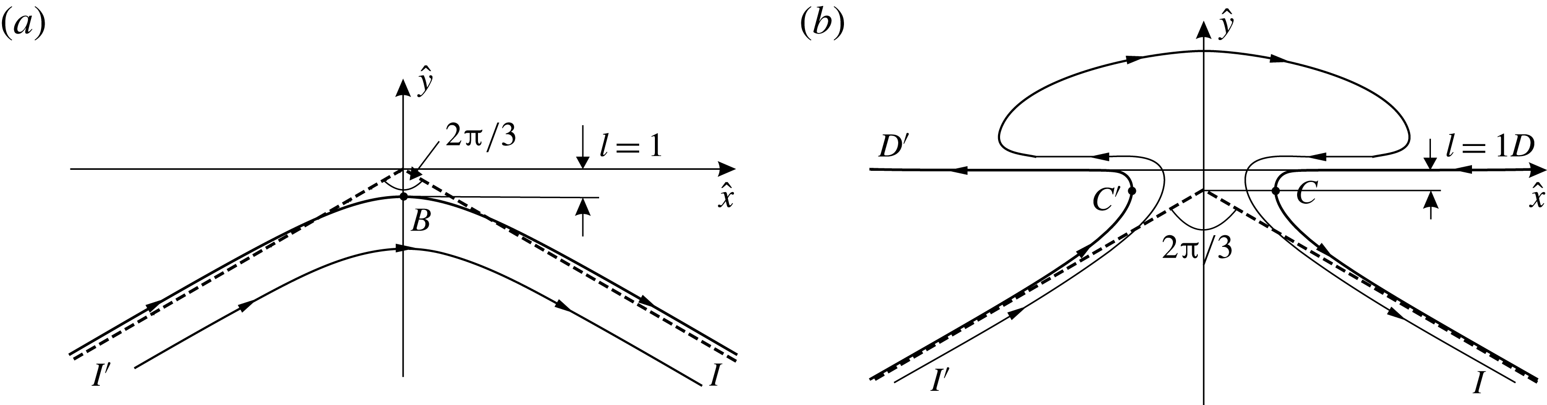
The sketches of the inner solutions for surface and interfacial waves are shown in figure 11. As one can see, these inner solutions are qualitatively different. For surface waves, the flow is similar to that in the angle of $120^{\circ }$ with a rounded apex. For the interfacial wave, the streamlines enter into the slot $C^{\prime }C$ between the inner crests and go out through the same slot; the points $D^{\prime }$ and $D$ at infinity are the stagnation ones with $\unicode[STIX]{x1D703}=\unicode[STIX]{x03C0}$ and $\unicode[STIX]{x1D703}=-\unicode[STIX]{x03C0}$ , respectively. On the streamlines $D^{\prime }C^{\prime }I^{\prime }$ and $DCI$ , the ordinate $y$ decreases monotonically from zero to $-\infty$ . For surface waves, the inner solution forms near the upper crest $B$ ; for interfacial waves, the inner solution does so near the inner crests $C$ and $C^{\prime }$ . It is also worthwhile to mention the difference between the asymptotes:

(6.16a,b ) $$\begin{eqnarray}\displaystyle {\hat{y}}=-\frac{|\hat{x}|}{\sqrt{3}}~\text{(for surface waves)},\quad {\hat{y}}=-\frac{|\hat{x}|}{\sqrt{3}}-1~\text{(for interfacial waves)}. & & \displaystyle\end{eqnarray}$$

For surface waves, the asymptote (6.16a ) was established by Longuet-Higgins & Fox (Reference Longuet-Higgins and Fox1977). For interfacial waves, according to figure 10, the asymptote (6.16a ) seems to be shifted by one unit downwards from the vertical benchmark $h_{0}=c^{2}/2$ . For surface waves, the asymptote always intersects the boundary close to the almost limiting configuration; for interfacial waves, according to figure 10, this seems not to be the case.

However, there exist some general features, namely, the vertical benchmarks for both flows are the same, $h_{0}=c^{2}/2$ ; the formulae for the natural scales are similar. In the dimensional form, they are as follows:

(6.17a,b ) $$\begin{eqnarray}\displaystyle l=\frac{q_{B}^{2}}{2g}~\text{(for surface waves)},\quad l=\frac{(q_{C}^{-})^{2}}{2g(1-\unicode[STIX]{x1D70C})}~\text{(for interfacial waves)}. & & \displaystyle\end{eqnarray}$$

In addition, the boundary conditions on the free surfaces $I^{\prime }BI$ and $I^{\prime }C^{\prime }D^{\prime }DCI$ are absolutely identical: both free surfaces are streamlines on which equation (6.9) of constant pressure is fulfilled.

6.4 Limiting configurations

The results obtained in §§ 6.2 and 6.3 allow us to predict easily the sketch of the limiting interfacial configuration. Indeed, it is evident that, for a fixed $\unicode[STIX]{x1D70C}$ , the limiting configuration takes place when the length $l$ defined by (6.15) is zero. Let $x_{C}$ be the abscissa of the inner crest $C$ . According to the last column of table 2, for the almost limiting interfacial waves $x_{C}\approx 3.7\times l$ . Hence if $l=0$ , then $x_{C}=0$ too. This means that the points $C$ and $C^{\prime }$ in figure 9(a) coincide. Moreover, at $l=0$ , the inner flow, whose sketch is shown in figure 11(b), shrinks to the point $C$ coinciding with $C^{\prime }$ . However, this shrinking conserves the directions of the slope $\unicode[STIX]{x1D703}$ at the infinitely remote points $D^{\prime }$ , $D$ and $I^{\prime }$ , $I$ . This reasoning naturally leads to the conclusion that the sketch of the limiting configuration is as shown in figure 9(b). The mushroom caps of the limiting interfacial configurations are stagnation zones consisting of the particles of the lower fluid.

Evidently, if $s_{C}$ is the arc-abscissa of point $C$ , then for the limiting configurations,

(6.18a-d ) $$\begin{eqnarray}\displaystyle \unicode[STIX]{x1D703}(s_{C}-0)=-\unicode[STIX]{x03C0},\quad \unicode[STIX]{x1D703}(s_{C}+0)=-\unicode[STIX]{x03C0}/6,\quad \unicode[STIX]{x1D703}(-s_{C}+0)=\unicode[STIX]{x03C0},\quad \unicode[STIX]{x1D703}(-s_{C}-0)=\unicode[STIX]{x03C0}/6. & & \displaystyle \nonumber\\ \displaystyle & & \displaystyle\end{eqnarray}$$

Thus for the limiting interfacial configurations, the function $\unicode[STIX]{x1D703}(s)$ is not continuous but has jumps at the points $\pm s_{C}$ . Therefore, the interface is not a smooth curve, proposition 1 is not true any more, and as follows from equations (6.18a,c ), $|\unicode[STIX]{x1D703}|_{max}=\unicode[STIX]{x03C0}$ for the limiting case.

If the density ratio $\unicode[STIX]{x1D70C}=1$ (Boussinesq limit), then the points $(-\unicode[STIX]{x03C0}/2,0)$ and $(\unicode[STIX]{x03C0}/2,0)$ are those of central symmetry for the left and right half of the interface, respectively. The limiting configuration in this case must be as predicted by Grimshaw & Pullin (Reference Grimshaw and Pullin1986, figure 9). The configuration contains a periodic stagnation zone formed by both the upper and lower fluids. The zone is bounded from above and below by the two free surfaces of the highest Stokes waves with angular crests that are oppositely directed and shifted by a half-period with respect to each other.

Figure 12.

(a) The dependences of $c^{2}$ on $H$ for different values of $\unicode[STIX]{x1D70C}$ from table 2. The upper parts of curves 1–3 (b) and 4–6 (c). The points indicate the pairs $(H,c^{2})$ for Holyer’s limiting configurations with $|\unicode[STIX]{x1D703}|_{max}=\unicode[STIX]{x03C0}/2$ (Holyer Reference Holyer1979).

6.5 The dependences of the phase speed on the wave steepness for interfacial waves

It is well known that, for surface waves, the wave steepness $H$ is one of the parameters that define the wave uniquely. As was shown by Grimshaw & Pullin (Reference Grimshaw and Pullin1986) and Turner & Vanden-Broeck (Reference Turner and Vanden-Broeck1986), for interfacial waves this is not the case. In figure 12(a), we demonstrate the dependences of $c^{2}$ on $H$ for different density ratios $\unicode[STIX]{x1D70C}$ . The correspondence between the numbered curves and the density ratios $\unicode[STIX]{x1D70C}$ can be found in table 2. For interfacial waves (numbers 2–14), the end points of all curves correspond to the almost limiting configurations with $\unicode[STIX]{x1D703}_{max}>179.98^{\circ }$ . As one can see, for $\unicode[STIX]{x1D70C}\geqslant 0.03$ , the wave steepness $H$ really does not define the wave uniquely. Another conclusion that can be drawn from figure 12(a) is that, generally, the phase speed $c$ decreases as the parameter $\unicode[STIX]{x1D70C}$ increases, but the fastest waves occur at $0.07\leqslant \unicode[STIX]{x1D70C}\leqslant 0.1$ . For the Boussinesq limit when $\unicode[STIX]{x1D70C}\rightarrow 1$ , the phase speed $c\rightarrow 0$ , and we do not number this graph.

The points in figure 12 correspond to the Holyer (Reference Holyer1979) limiting configurations ( $|\unicode[STIX]{x1D703}|_{max}=\unicode[STIX]{x03C0}/2$ ). Accurate values of the pairs $(H,c^{2})$ for the Holyer limit are presented in table 3.

Let us consider the case of small $\unicode[STIX]{x1D70C}$ in more detail. The upper parts of curves 1–3 of figure 12(a) are shown in figure 12(b). Curve 2 demonstrates that at $\unicode[STIX]{x1D70C}=0.01$ the pair $(H,c^{2})$ defines the wave uniquely, but already at $\unicode[STIX]{x1D70C}=0.03$ (curve 3) the uniqueness disappears. Curves 4–6 of figure 12(c) prove that, for $0.07<\unicode[STIX]{x1D70C}\leqslant 0.1$ , the dependences $c^{2}$ versus $H$ have points of self-intersection, which means that in this range of $\unicode[STIX]{x1D70C}$ there exist waves which have identical values of the wave steepness $H$ and the phase velocity  $c$ but different shapes. Two such waves at $\unicode[STIX]{x1D70C}=0.1$ are displayed in figure 13. For the sake of comparison, the $x$ -axis here is located at equal vertical distances from the crest and trough ( $y_{B}=-y_{A}$ ). The values of the parameters $P$ , $|\unicode[STIX]{x1D703}|_{max}$ , $H$ and $c^{2}$ for these two waves are shown in table 4.

Figure 13.

Two waves with the same $H$ and $c^{2}$ at $\unicode[STIX]{x1D70C}=0.1$ .

Table 3.

The pairs $(H,c^{2})$ for Holyer’s limiting configurations with $|\unicode[STIX]{x1D703}|_{max}=\unicode[STIX]{x03C0}/2$ (Holyer Reference Holyer1979).

Table 4.

The parameters $P$ , $|\unicode[STIX]{x1D703}|_{max}$ , $H$ and $c^{2}$ for two waves of figure 13.

7.1 Comparison with the work by Saffman & Yuen (Reference Saffman and Yuen1982)

Accurate computations of interfacial waves of moderate steepness were carried out by Saffman & Yuen (Reference Saffman and Yuen1982). In table 2 of their paper, these authors presented the values of the phase speed

(7.1) $$\begin{eqnarray}\displaystyle C=c\sqrt{\frac{1+\unicode[STIX]{x1D70C}}{1-\unicode[STIX]{x1D70C}}}=\sqrt{\frac{2(1+\unicode[STIX]{x1D70C})}{k}} & & \displaystyle\end{eqnarray}$$

versus $2\unicode[STIX]{x03C0}H$ for the density ratio $\unicode[STIX]{x1D70C}=0.1$ . As follows from (3.1), $C$ is the dimensionless phase speed non-dimensionalized with respect to the phase speed of infinitesimal waves. In table 5 (second column), we have reproduced the results by Saffman & Yuen (Reference Saffman and Yuen1982). The third to fifth columns present our computations of $C$ at $N=800$ , 1600 and 3200, where $N$ is the number of points which approximate the right half of the interface $L_{2\unicode[STIX]{x03C0}}$ .

Generating the data of table 2, Saffman & Yuen (Reference Saffman and Yuen1982) thoroughly checked their decimals, and as one can see from table 5, their check turns out to be very efficient because all these decimals are correct. In our computations, we consider $N=800$ as a working point number which allows us to compute the interfacial waves for any $0<\unicode[STIX]{x1D70C}\leqslant 1$ in the range $0<|\unicode[STIX]{x1D703}|_{max}\leqslant 179.98^{\circ }$ with an error less than $10^{-8}$ . Table 5 confirms that at $N=800$ we have at least eight correct decimals and at the same time demonstrates an explicit convergence of the algorithm as $N$ increases. The last column of table 5 shows the values of $|\unicode[STIX]{x1D703}|_{max}$ in order to give the reader a representation about the closeness of the waves to the limiting configuration.

At $N=800$ , the time for computing one wave is only several seconds but certainly the time increases with increase of $N$ . Nevertheless, all data of table 5 have been generated for approximately one hour on the notebook HP G1 EliteBook Folio 1040.

Table 5.

Continuation of table 2 from the paper by Saffman & Yuen (Reference Saffman and Yuen1982, S&Y) ( $\unicode[STIX]{x1D70C}=0.1$ ).

7.2 Comparison with the work by Turner & Vanden-Broeck (Reference Turner and Vanden-Broeck1986)

In the paper by Turner & Vanden-Broeck (Reference Turner and Vanden-Broeck1986), the most extensive numerical data were obtained for the case $\unicode[STIX]{x1D70C}=0.1$ . The results were displayed in figure 2 (p. 374) of their paper and a copy of this figure is shown in figure 14(a). In the notation used by Turner & Vanden-Broeck, $s$ is the wave steepness $H$ , and $\unicode[STIX]{x1D707}$ is the squared phase velocity  $c^{2}$ . As one can see from figure 14(a), the authors indicate on the curve five characteristic points:

1. (i) a non-overhanging wave;

2. (ii) the wave for the Holyer limit;

3. (iii) the wave with the greatest overhang;

4. (iv) a wave with a slight overhang; and

5. (v) a non-overhanging wave similar to the wave (ii).

On the basis of these computations, the authors conjectured (p. 371) that ‘an alternation between non-overhanging and overhanging waves continues indefinitely as one proceeds along the solution branch’. We have digitized the graph of figure 14(a) and plotted it together with our results in figure 14(b). As one can see, our computations do not confirm the conjecture by Turner & Vanden-Broeck (Reference Turner and Vanden-Broeck1986), but as was demonstrated in § 6.4, they confirm the conjecture by Saffman & Yuen (Reference Saffman and Yuen1982) that the overhanging waves continue to exist until the interface starts to touch itself.

Figure 14.

(a) A copy of figure 2 from the paper by Turner & Vanden-Broeck (Reference Turner and Vanden-Broeck1986). (b) Comparison of our results with those in (a): the point indicates the Holyer limit; squares correspond to the data of table 5.