


1. Introduction
Vote trading, also commonly known as logrolling, is a cornerstone of the analysis of politicians’ behavior in collective decision making. As a form of hidden cooperation between legislators with typically opposing political views, vote trading is crucial to the legislative process, for better or for worse.
Reciprocity is an obvious aspect of the cooperative behavior in which two legislators engage when voting in favor of each others’ preferred bills to secure the passage of both bills (Cohen and Malloy, Reference Cohen and Malloy2014, Stratmann, Reference Stratmann1992, Reference Stratmann1995). As a logical consequence, vote trading leaves behind reciprocity patterns in voting records (Buchanan and Tullock, Reference Buchanan and Tullock1962; Weingast and Marshall, Reference Weingast and Marshall1988). As we will argue, accounting for such patterns is a necessary condition for any valid estimation of vote trading, a condition that is not properly considered by existing empirical approaches. We propose a conceptual and methodological framework to find and quantify the prevalence of such patterns, facilitating the estimation of vote trading at scale. Our method helps to establish statistically whether a pattern of reciprocity present in the data is sufficient to be considered evidence for a given theory of vote trading. Arguably, quantitatively documenting reciprocal patterns in voting favors is a crucial aspect of providing evidence on vote trading. In addition, our contribution can serve as an independent tool to empirically search for situations in voting data in which vote trading (according to a given theory) is likely to have occurred.
Our proposal is broadly applicable and builds on three well-accepted theoretical principles: (1) traded votes involve legislators’ deviations from their expected voting behavior, (2) these deviations benefit specific legislators (i.e., they are favors to other legislators), and (3) these favors are systematically reciprocated. Building on the concept of reciprocity in directed weighted networks, our framework incorporates these three principles and provides an index quantifying the prevalence of vote trading. In contrast to the existing econometric approaches, the logrolling index works in large-scale contexts where domain knowledge (to specify the regression model) might be difficult or impossible to obtain.
In a few words, the method constructs a network linking the deviating legislators (deviators, i.e., those that would not vote Yes in the absence of a trade) to legislators who exhibit strong preferences for the passage of the respective bill (beneficiaries). Then, it assesses whether the resulting network of directed deviations yields systematic reciprocity. Our approach follows the most prominent previous empirical contributions Cohen and Malloy (Reference Cohen and Malloy2014); Stratmann (Reference Stratmann1992, Reference Stratmann1995) in that it exclusively focuses on trades between pairs of legislators. With this focus, we do not suggest that trades between factions/groups of legislators or trades between more than two individuals (e.g., trades in the form of triads) are less important in legislative politics. It is simply that non-dyadic trade is not the focus of our inquiry and neither the object of the seminal empirical studies on vote trading to which we apply our framework.
We see our contribution as an important addition to the existing literature as it directly builds on its theoretical foundations and is particularly useful to assess the prevalence of vote trading between legislators, which is very challenging due to its “hidden” nature. Strategically offering one’s vote to a fellow legislator with opposing political views may contrast with the expectation of voters and peers, so legislators on both sides of a vote-trading agreement are keen to keep such deals secret.Footnote 1 Hence, quantifying vote trading requires us to measure something that is not directly observable.
Econometric analysis has proven useful to test the existence of vote trading among small sets of votes, given specific prior information about the presence of vote-trading coalitions (qualitatively reported) (Esteves and Mesevage, Reference Esteves and Mesevage2021; Stratmann, Reference Stratmann1992, Reference Stratmann1995). It has also proven useful in the context of broadly applicable theories of vote trading, allowing the consideration of several years of roll call voting across a wide spectrum of policy issues (Cohen and Malloy, Reference Cohen and Malloy2014). The previous empirical studies do not explicitly capture a key theoretical aspect of vote trading: the reciprocal exchange of votes between legislators favoring specific bills. Nevertheless, they agree with the notion that this form of reciprocity is a central aspect of legislative vote trading. Arguably, reciprocity in voting favors is the very essence of vote trading.Footnote 2
We validate the method with an agent-based model of the legislative process. In this setting, we have full control over the propensity to trade votes and can identify true positives in the outcome data, enabling the measurement of the “ground truth”. The proposed logrolling index exhibits a strong correlation with the ground truth and is robust to significant levels of noise in the data as well as sample sizes.
We apply the method to study vote trading in two different, previously investigated, settings: one in the U.S. Senate: Cohen and Malloy (Reference Cohen and Malloy2014), and one in the U.S. House: Stratmann (Reference Stratmann1992). The first application validates Cohen and Malloy (Reference Cohen and Malloy2014)’s theory and empirical findings of vote trading and provides more nuance with regard to its limitations. In the second application, we deploy our method to estimate the prevalence of vote trading across time. In both applications, we find richer, yet consistent evidence of vote trading in U.S. politics.
The paper is structured in the following way. Section 2 discusses the historical relevance of vote trading and the literature on the topic. Section 3 introduces the methodology, and Section 4 validates it. In Sections 5 and 6, we present the two empirical applications. Finally, Section 7 discusses the method’s limitations and provides concluding remarks.
2. Background and literature
Historical anecdotal evidence suggests that vote trading plays an important role in legislative politics (Bordewich, Reference Bordewich2016; Casson, Reference Casson2009; Kingdon, Reference Kingdon1989; Pastor, Reference Pastor1982; Schraufnagel, Reference Schraufnagel2011). For example, Kingdon (Reference Kingdon1989, p. 100) quotes a statement of an anonymous representative regarding their traded vote on a bill deregulating cigarette advertisement:
“This will be sort of a buddy vote. I know cigarettes are harmful and I wouldn’t touch them myself. But a lot of my friends are concerned about this, because tobacco means a lot to the economy of their areas. They do things for me when I need it, and I’ll do this for them. Frankly, it’s just a matter of helping out your friends.”
Historical records mentioning vote trading date back to the first U.S. Congress in 1789 (Bordewich, Reference Bordewich2016).Footnote
3
In the early 19th century, James K. Polk (U.S. President and former Speaker of the House) reportedly “stood against the practice of logrolling, or vote trading, considering it a form of corruption” (Schraufnagel, Reference Schraufnagel2011, p. 170). Reports of recent vote trading in the U.S. Congress often describe these activities in the context of special-interest politics. A well-known example is the (failed) congressional attempt to revise tariffs to trigger an economic boost during the Great Depression. It led President Herbert Hoover to conclude that “[c]ongressional [tariff] revisions [
 $\ldots$
] with all their necessary collateral surroundings in lobbies, logrolling and the activities of group interests, are disturbing to public confidence” (Pastor, Reference Pastor1982, p. 69).
More broadly, the very incentives that make vote trading attractive—that legislators care intensely about policies affecting specific industries, regions, or constituent groups—are themselves well-documented in the literature on economic policymaking and legislative behavior (Carnes and Lupu, Reference Carnes and Lupu2023; Grossman and Helpman, Reference Grossman and Helpman1994; Levitt, Reference Levitt1996; Kalt and Zupan, Reference Kalt and Zupan1984; Peltzman, Reference Peltzman1984). In addition, other accounts of the historical relevance of vote trading in Europe highlight its importance in the context of heterogeneous local interests and catering to the legislators’ electoral districts (see, for example, Casson (Reference Casson2009) for the case of UK railways constructions, and Kriesi and Trechsel (Reference Kriesi and Trechsel2008) for trades between representatives of different Swiss cantons).
Early scientific inquiry into the nature and importance of vote trading dates back to Arthur Bentley’s work (Bentley, Reference Bentley1908). Since then, a substantive theoretical body of literature on the issue has emerged (Bernholz, Reference Bernholz1974, Reference Bernholz1978; Buchanan and Tullock, Reference Buchanan and Tullock1962; Casella et al., Reference Casella, Palfrey and Turban2014; Casella and Palfrey, Reference Casella and Palfrey2019; Haefele, Reference Haefele1970; Mueller, Reference Mueller2003; Riker and Brams, Reference Riker and Brams1973; Shepsle and Weingast, Reference Shepsle and Weingast1981; Tullock, Reference Tullock1970; Wilson, Reference Wilson1969). Studies on vote trading distinguish two particular forms: implicit and explicit trades. Implicit vote trading refers to exchanging favors at the drafting stage of so-called “omnibus bills”, resembling a package of policies favoring different groups and, thereby, ensuring passage of all policies in one vote (“trades” thus take place within the same piece of legislation). Explicit vote trading refers to legislators voting in favor of each other’s preferred bills (or amendments on bills) to ensure minimal winning coalitions in every roll-call involved in the trade. Most empirical studies—as well as our framework—focus on explicit vote trading, whereby legislators trade with each other by voting in favor of each other’s favorite bills.Footnote 4
Empirical studies on vote trading are scarce and can be classified into three types. The first consists of laboratory experiments (Casella et al., Reference Casella, Palfrey and Turban2014; Casella and Macé, Reference Casella and Macé2021; Eckel and Holt, Reference Eckel and Holt1989; McKelvey and Ordeshook, Reference McKelvey and Ordeshook1980). These studies focus on testing the micro-mechanisms that elicit incentives to trade votes in controlled environments. Second, there are interview studies, as well as case studies based on anecdotal evidence (see, e.g., Wright, Reference Wright, Wright, Rieselbach and Dodd1986). Finally, the third type consists of econometric work (Cohen and Malloy, Reference Cohen and Malloy2014; Kau and Rubin, Reference Kau and Rubin1979; Stratmann, Reference Stratmann1992, Reference Stratmann1995). These studies test hypotheses on how roll-call data would look in the absence of vote trading. Several empirical contributions investigate other forms of vote trading. For instance, Akzoy (Reference Akzoy2012) studies implicit logrolling (“within-legislation logrolling”) in the European Union’s Council of Ministers as part of a bargaining process over individual pieces of legislation. Kardasheva (Reference Kardasheva2013), also focusing on E.U. legislative politics investigates intercameral logrolling in the form of package deals framed in exchange between the European Parliament and the Council of Ministers. Most recently, Esteves and Mesevage (Reference Esteves and Mesevage2021) study the specific historical setting of logrolling between parliamentary subcommittees within the issue of the approval of new railway routes in 19th-century Great Britain.
As we have previously mentioned, the existing econometric work is typically conducted on a small scale as it requires extensive contextual knowledge to specify statistical models. Our framework overcomes this limitation by providing a method to estimate the prevalence of vote trading on a large scale, enabling, for example, the temporal study of vote trading. In the next section, we guide the reader through the framework.
3. Methodological framework
Our framework builds on three well-accepted theoretical principles: (1) traded votes involve legislators’ deviations from their expected voting behavior, (2) these deviations benefit specific legislators (i.e., they are favors to other legislators), and (3) these favors are systematically reciprocated (Axelrod, Reference Axelrod1984; Buchanan and Tullock, Reference Buchanan and Tullock1962; Mueller, Reference Mueller2003; Tullock, Reference Tullock1970; Weingast and Marshall, Reference Weingast and Marshall1988). Closely following these theoretical pillars, the core of our framework consists of two types of data. First, we use data on votes that are considered deviations from the usual behavior (first data type) to construct a network linking such deviations to legislators who have signaled strong preferences for the passage of the respective bill (second data type). Second, we assess—statistically—whether the resulting network of directed deviations yields a systematic pattern of reciprocity.
3.1 A networks perspective on vote trading
Before introducing the framework, we fix some notation conventions used throughout the paper. A “tuple”
 $(i,k)$
denotes a legislator
 $i$
and a roll-call
 $k$
, and indicates a relationship between the two (for example, a Yes vote). A tuple of tuples such as
 $((i,k),(j,l))$
represents a pair of such relationships—for example, legislator
 $i$
voting in roll-call
 $k$
and legislator
 $j$
voting in roll-call
 $l$
. Bold capitalized characters denote sets, typically of tuples; hollow capitalized characters denote matrices. The three matrices central to the framework are
 $\mathbb{Q}$
(predicted Yes-vote probabilities, the operational definition of expected behavior),
 $\mathbb{D}$
(deviations from those expectations), and
 $\mathbb{P}$
(revealed preferences over bills); each matrix is defined in turn below.
3.1.1 The empirical problem
The empirical problem of measuring the prevalence of vote trading in roll-call data can be generalized as follows. For a specific legislature, we want to assess whether vote trading can explain some of the voting decisions cast in the
 $K$
roll calls during a given period. The starting point is a set
 $\mathbf{V}$
with all Yes roll-call decisions from
 $N$
legislators voting in
 $K$
roll-calls. We then construct two further sets: a set
 $\mathbf{D} \subseteq \mathbf{V}$
of Yes votes considered deviations from the expected behavior of the corresponding legislators (for example, a legislator voting Yes on a bill their party or constituency would typically oppose), and a set
 $\mathbf{P}$
of tuples
 $(i,l)$
indicating that legislator
 $i$
has revealed strong preferences in favor of bill
 $l$
via, for example, signals such as bill sponsorships.
The key intermediate step is that the empirical model used to construct
 $\mathbf{D}$
implicitly imposes constraints that filter which votes are classified as expected versus deviant. This filtering, combined with the signaling structure embedded in
 $\mathbf{P}$
, delimits which vote pairs
 $((i,k),(j,l))$
can constitute a reciprocal exchange. A trade would appear in the data as a tuple
 $((i,k),(j,l))$
such that
 $(i,k) \in \mathbf{D}$
,
 $(j,l) \in \mathbf{D}$
,
 $(i,l) \in \mathbf{P}$
,
 $(j,k) \in \mathbf{P}$
,
 $(i,k) \notin \mathbf{P}$
, and
 $(j,l) \notin \mathbf{P}$
. That is,
 $i$
deviates on a bill that
 $j$
strongly supports, and vice versa. If no reciprocal patterns are found in the data, none of the observed voting decisions can be explained by vote-trading. If they are found, the question becomes whether the pattern is systematic enough to rule out chance; this is what the logrolling index (Subsection 3.2) formalizes.
Constructing
 $\mathbf{D}$
and
 $\mathbf{P}$
—and deciding which roll calls to consider in the first place—are the three substantive design choices the researcher must make. We discuss each one before turning to the logrolling index itself.
3.1.2 Design choice 1: Identifying deviations (
 $\mathbf{D}$
)

A deviation is a Yes vote that cannot be accounted for by the usual determinants of a legislator’s voting behavior (party, constituency, ideology, and so on). Operationally, “expected” behavior is encoded in a matrix
 $\mathbb{Q}$
of size
 $N \times K$
, where
 $\mathbb{Q}_{ik}$
is the model-implied probability that legislator
 $i$
would vote Yes on roll call
 $k$
in the absence of vote trading.
 $\mathbf{D}$
is then constructed by flagging Yes votes whose corresponding
 $\mathbb{Q}_{ik}$
is low enough to be considered against expectation (we operationalize this in Design choice 3). The framework is agnostic about how
 $\mathbf{D}$
is constructed: one could use an econometric model, a black-box prediction approach from machine learning, or ideal-point estimates such as DW-NOMINATE (Clinton et al., Reference Clinton, Jackman and Rivers2004; Poole and Rosenthal, Reference Poole and Rosenthal1985). A caveat specific to ideal-point scores is that they are fit on the full roll-call matrix, including votes that may themselves reflect trading, so using them as
 $\mathbb{Q}$
risks absorbing trading behavior into the estimated ideal points. In the applications below we embed the econometric specifications of the original studies (Cohen and Malloy, Reference Cohen and Malloy2014; Stratmann, Reference Stratmann1992, Reference Stratmann1995) to maintain direct comparability with their identification strategies. The identification requirement at this step is modest but substantive: variables that themselves operationalize the specific trading mechanism under investigation should be withheld from
 $\mathbb{Q}$
, even at the cost of some predictive accuracy, because including them would absorb the reciprocal behavior that the index is designed to detect. In each application below we state explicitly which covariates are included for this reason and which are withheld.
3.1.3 Design choice 2: Identifying revealed preferences (
$\mathrm{P}$
)

Constructing
 $\mathbf{P}$
requires the researcher to commit to a specific theory of vote trading, because
 $\mathbf{P}$
operationalizes what it means for a legislator to “strongly support” a bill. In practice,
 $\mathbf{P}$
is populated from observable signals of strong preference—such as bill sponsorship or cosponsorship, amendment authorship, or theory-implied alignment with a legislator’s district or state interests—selected to match the theory under investigation. For example, Cohen and Malloy (Reference Cohen and Malloy2014) theorize that U.S. Senators trade votes on bills highly relevant to their states’ major industries—a premise consistent with a large body of evidence that legislators’ roll-call behavior tracks constituency economic interests (Carnes and Lupu, Reference Carnes and Lupu2023; Levitt, Reference Levitt1996; Peltzman, Reference Peltzman1984). There,
 $\mathbf{P}$
records which bills are relevant to which senators’ states. Stratmann (Reference Stratmann1992)’s theory of amendment-based trading among special-interest representatives instead suggests
 $\mathbf{P}$
should record amendment sponsorships. Different theories yield different
 $\mathbf{P}$
s and thus different implied trade structures. This is by design: our framework provides a common architecture for testing theory-specific predictions about reciprocal voting, not a theory-free detector of vote trading.
3.1.4 Design choice 3: Restricting to narrow-outcome votes
Theories of vote trading typically imply that trades occur precisely when an additional Yes vote can plausibly change the outcome—that is, on bills with narrow expected margins (Cohen and Malloy, Reference Cohen and Malloy2014; Stratmann, Reference Stratmann1992). When the theory under investigation carries this implication, the researcher restricts
 $\mathbf{D}$
to deviations occurring in narrow-outcome roll calls. Operationally, this combines two cuts: a model-based cut (
 $\mathbb{Q}_{ik}\lt 0.5$
, so that the legislator was expected to vote No) and an observed-margin cut (the realized vote margin is narrow enough that an additional Yes could plausibly have flipped the outcome). We apply this restriction in both applications.Footnote
5
3.1.5 Relation to regression-based approaches
Previous empirical contributions do not explicitly require reciprocity. They filter
 $\mathbf{V}$
on legislator and bill characteristics and regress voting outcomes on these covariates; a significant coefficient (or combination) is interpreted as evidence consistent with vote trading. This approach is informative about whether vote trading may explain some observed votes, but it does not identify which pairs of legislators are trading. Our framework complements this: it builds the potential trade structure explicitly by linking specific legislators on specific bills and asks whether the resulting network exhibits more reciprocity than chance would predict. The two approaches are compatible. In both applications we embed a regression model (to construct
 $\mathbf{D}$
) inside the network framework, and both applications relate to prior work that relied exclusively on regression-based approaches.
3.1.6 From sets to the networks
Combining
 $\mathbf{D}$
and
 $\mathbf{P}$
, we construct a directed weighted network between legislators, which we call the directed deviation network (DDN). A weighted edge from
 $i$
to
 $j$
indicates that
 $i$
deviated in at least one roll call where
 $j$
explicitly signaled support for the corresponding bill. Whether the DDN exhibits systematic reciprocity—beyond what the data structure alone would produce—is what our index, developed next, quantifies.
3.2 Logrolling index
Let us switch from sets to matrices and define
 $\mathbb{D}$
and
 $\mathbb{P}$
, both of size
 $N \times K$
.
 $\mathbb{D}_{ik}=1$
indicates a deviation of
 $i$
in roll call
 $k$
(zero otherwise) and
 $\mathbb{P}_{jl}=1$
indicates a revealed preference of
 $j$
in favor of bill
 $l$
(zero otherwise). From them, we construct a weighted adjacency matrix
 \begin{equation} \mathbb{W} = \mathbb{D} \bullet \mathbb{P}', \end{equation}
containing counts of directed deviations between legislators.
 $\mathbb{W}$
is the adjacency matrix of the DDN. We treat each contested bill as most strongly preferred by a single legislator.Footnote
6
Building on the concept of reciprocity in directed weighted networks (Garlaschelli and Loffredo, Reference Garlaschelli and Loffredo2004; Squartini et al., Reference Squartini, Picciolo, Ruzzenenti and Garlaschelli2013), we define the level of reciprocity between legislators
 $i$
and
 $j$
as
 \begin{equation} w_{ij}^{\leftrightarrow } = \min \left [\mathbb{W}_{ij} , \mathbb{W}_{ji} \right ] = w_{ji}^{\leftrightarrow }, \end{equation}
and the aggregate proportion of reciprocity across all legislators as
 \begin{equation} r = \frac {\sum _{i}\sum _{j} w_{ij}^{\leftrightarrow }}{\sum _{i}\sum _{j} \mathbb{W}_{ij}}. \end{equation}
A high
 $r$
is not by itself evidence of vote trading: the DDN may be reciprocal simply because it is dense, or because
 $\mathbb{P}$
concentrates attention on a subset of legislators who are active across many bills. Hence, we compare
 $r$
to the reciprocity
 $\bar {r}_0$
expected under a null model that preserves the structural features that are unrelated to trading. The framework is agnostic about the specific null model; it requires only that an ensemble
 $r_{0,1}, \ldots , r_{0,T}$
can be generated, from which
 \begin{equation} \bar {r}_0 = \frac {1}{T} \sum _{t=1}^T r_{0,t}. \end{equation}
The null model should preserve the structural features of the data that are not themselves indicative of vote trading. In practice, this means mirroring the controls used to construct
 $\mathbf{D}$
, so that any reciprocity attributable to those controls is absorbed by the null rather than credited to trading. In both applications we generate random DDNs through a procedure that is consistent with the control structure of the specification used to construct
 $\mathbf{D}$
(see Section 5). The logrolling indexFootnote
7
is
 \begin{equation} \ell = \frac {r - \bar {r}_0}{1 - \bar {r}_0}. \end{equation}
Interpreting
 $\ell$
. The index is bounded above by
 $1$
and behaves, on the positive side, analogously to a correlation coefficient (Garlaschelli and Loffredo, Reference Garlaschelli and Loffredo2004; Squartini et al., Reference Squartini, Picciolo, Ruzzenenti and Garlaschelli2013). A value of
 $\ell = 0$
means the DDN’s reciprocity is no greater than what the null produces; positive values indicate systematically more reciprocal deviations than chance; values close to
 $1$
indicate that almost every favor is repaid in kind. We interpret
 $\ell$
as the tendency of a legislative context to sustain cooperative behavior through vote trading when the opportunity arises—different contexts may produce different numbers of candidate trades (e.g., because the prevalence of narrow-margin votes varies), and
 $\ell$
measures the proportion of those opportunities that are reciprocated rather than the raw count. A context in which vote trading is not a recurrent cooperation mechanism would therefore yield an index close to zero (or even negative), consistent with a deviation structure generated by non-cooperative behavior.
Two caveats follow. First, the index measures prevalence, not incidence: it does not identify which specific dyads traded, only whether the overall pattern of reciprocity exceeds chance.Footnote 8 Second, interpreting a given magnitude requires context—how many deviations there are, when they occur, who produces them, and on what topics—which is why we accompany both applications with descriptive analyses of the reciprocal portion of the DDN.
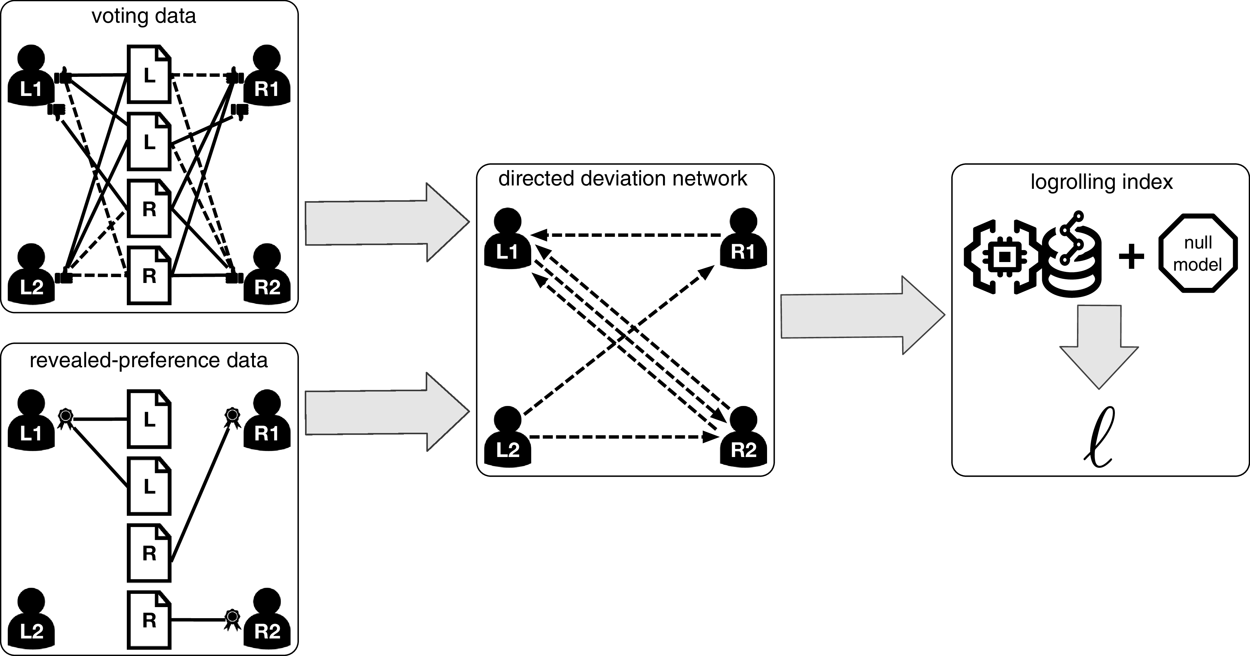
Figure 1 summarizes the full pipeline, from raw voting data through the DDN to the reciprocal component underlying
 $\ell$
.
Pipeline of the methodology.

Figure 1 Long description
Panel A: A network diagram showing voting data with legislators labeled L1, L2, R1, and R2 connected by lines representing voting patterns. Panel B: A network diagram showing revealed-preference data with similar connections. Panel C: A directed deviation network diagram with arrows indicating the direction of voting influence between legislators. Panel D: A logrolling index diagram combining data and a null model to calculate the index.
3.3 Interpretive scope of the logrolling index
Because
 $\ell$
is a statistical measure rather than a direct observation of trades, it is worth stating which processes would be ruled out by a positive value and which ones would not. The null
 $\bar {r}_0$
eliminates reciprocity arising from individual-level heterogeneity in deviation propensities: because null deviations are drawn from
 $\mathbb{Q}$
independently—which absorbs party, constituency, ideology, and the other covariates used to construct
 $\mathbb{D}$
—any reciprocity driven by particular legislators deviating more often is already accounted for.
What the null does not eliminate is reciprocity arising from dyad-level coordination that is not captured by
 $\mathbb{Q}$
. Candidate alternatives include faction- or coalition-based coordination and centralized leadership-mediated matching of reciprocal deviations across bills. Whipping, for example, is a top-down, one-directional process and cannot by itself produce the signal: it would do so only if it also matched specific legislators into pairs whose costly deviations land on each other’s sponsored bills—that is, only if it operated as a dyad-matching mechanism. Under our framework, however, any such process must still produce costly deviations (against the predicted vote), directed specifically at each other’s preferred bills, and systematically reciprocal beyond the null. A process satisfying all three conditions is, from our viewpoint, functionally equivalent to reciprocal favor exchange in voting; it differs from explicit dyadic logrolling only in the coordination mechanism. Accordingly, we interpret
 $\ell$
as measuring systematic reciprocal favor exchange in voting consistent with dyadic logrolling, rather than as a direct identifier of explicit pairwise trades. The next section validates the index against ground-truth vote-trading rates generated by an agent-based model.
4. Validation
Validating our method entails showing that the logrolling index exhibits a strong positive correlation with a direct measurement of vote trading. Furthermore, such a relationship should be robust across different institutional settings, i.e., across different scales and structures of
 $\mathbb{D}$
and
 $\mathbb{P}$
, as well as with varying levels of noise introduced in
 $\mathbb{Q}$
. For this purpose, we develop an agent-based model of vote trading where we control the propensity to trade votes and directly measure the ground truth: the fraction of deviations that are the result of trading votes.
4.1 Model components
The model consists of
 $N$
agents and
 $K$
roll calls that are voted sequentially. Matrix
 $\mathbb{Q}$
encodes the probabilities of each agent voting Yes in each roll call.
 $\mathbb{Q}$
is generated by drawing random numbers from a uniform distribution. Each bill has one agent who reveals its preference for its passage by explicitly supporting it.Footnote
9
This information is encoded in
 $\mathbb{P}$
, where 1 means support and zero otherwise. Note that
 $\mathbb{P}$
is public information, so all agents can see who supports each bill. Matrix
 $\mathbb{P}$
is generated randomly, with every agent having the same probability of supporting a bill. Finally, a Yes vote is considered a deviation only if its corresponding voting probability is
 $\mathbb{Q}_{ik} \lt 0.5$
, so it is encoded as
 $\mathbb{D}_{ik}=1$
. One final setup step ensures consistency between
 $\mathbb{Q}$
and
 $\mathbb{P}$
by ensuring that agent
 $i$
sponsoring a bill
 $k$
has probability of a Yes vote
 $\mathbb{Q}_{ik} = 1$
. As the model proceeds, the agents engage in vote trading and generate random deviations, filling
 $\mathbb{D}$
.
4.2 Model dynamics
To control the amount of vote trading produced by the agents, we specify a parameter
 $\delta \in (0,1)$
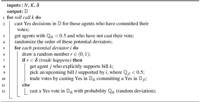
that captures the overall prevalence of this activity. Let us explain the model algorithm to make clear how
 $\delta$
determines the prevalence of vote trading. Each period, a bill
 $k$
is voted. Agent
 $i$
casts a Yes vote if they already committed this vote due to a previously arranged vote trade. If the vote has not been committed and if
 $\mathbb{Q}_{ik}\lt 0.5$
, then agent
 $i$
is a potential deviator in roll call
 $k$
. With probability
 $\delta$
,
 $k$
’s supporter, agent
 $j$
, approaches agent
 $i$
and they arrange a trade where
 $j$
commits a future deviation in a roll call where
 $i$
supports the corresponding bill. If there is no trade, then
 $i$
casts a Yes in roll call
 $k$
with probability
 $\mathbb{Q}_{ik}$
. The pseudocode of the model is provided in Algorithm 1.
Vote-trading model pseudocode

Algorithm 1 Long description
An equation with inputs epsilon ext, epsilon mag, Q, P, D and output new logrolling index. The algorithm iterates over each entry in Q, drawing a random number r between 0 and 1. If r is less than epsilon ext, it generates noise magnitude xi, draws a random number s between -1 and 1, rescales xi, and updates Qik. If Qik is greater than 0.5 and Dik is 1, Dik is set to 0. Finally, the new logrolling index is computed.
One instantiation of the model yields a deviation matrix
 $\mathbb{D}$
. In the real world, one cannot observe
 $\delta$
but only the realized deviations. In the model, we can identify those deviations in
 $\mathbb{D}$
that are the result of vote trading. Hence, once
 $\mathbb{D}$
has been computed, we define the ground truth as the share of deviations that were produced by trading. The validation of the index consists of finding a strong positive association between the logrolling index and the ground truth.
4.3 Validation results
In Figure 2, we present the outcomes of this validation. Each data point corresponds to a single run of the model. A model run takes
 $N$
,
 $K$
, and
 $\delta$
as inputs, generates
 $\mathbb{Q}$
and
 $\mathbb{P}$
randomly, and returns
 $\mathbb{D}$
. Then, the ground truth and the logrolling index are computed. Each panel shows different model runs for random values of
 $\delta$
to generate variation in the ground truth. We present the validation separating parameterizations with different
 $N$
s and
 $K$
s. All panels present a strong positive correlation, which validates the logrolling index. Even in a small-size setting (
 $N=10$
and
 $K=10$
), this relationship holds (higher volatility in the index is expected under a small sample as with every statistical method).
Logrolling index and vote-trading ground truth.

In empirical applications,
 $\mathbb{Q}$
and
 $\mathbb{P}$
are constructed from data following the design choices laid out in Section 3; Sections 5 and 6 provide the specifics for our two cases. Because
 $\mathbb{Q}$
is the component estimated stochastically rather than specified by design, it is the natural target for a sensitivity analysis. Hence we assess how robust the logrolling index is to noise in
 $\mathbb{Q}$
.
When analyzing potential noise in
 $\mathbb{Q}$
, there are two dimensions to be considered: (1) the extent
 $\epsilon _{ext}$
and (2) the magnitude
 $\epsilon _{mag}$
. The noise extent captures how many entries in
 $\mathbb{Q}$
can be noisy. The noise magnitude represents the maximum absolute size of the distortions in
 $\mathbb{Q}$
, which could be positive or negative. To analyze the bias in the logrolling index induced by noise, we use the data generated for Figure 2. More specifically, we take outputs in which
 $\delta \approx 0.5$
for each one of the four cases combining
 $N$
and
 $K$
.
The analysis consists of defining
 $\epsilon _{ext}$
and
 $\epsilon _{mag}$
, generating noise in
 $\mathbb{Q}$
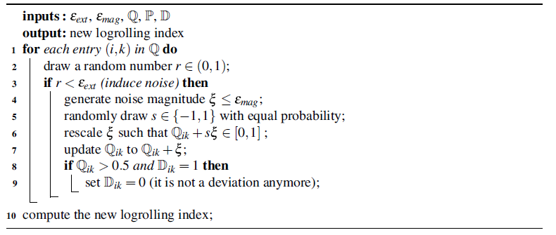
, re-estimating the logrolling index, and computing the bias as the difference between the new index and the one without noise. Algorithm 2 provides the pseudocode of this procedure for a combination of
 $\epsilon _{ext}$
and
 $\epsilon _{mag}$
. For given parameters
 $N$
,
 $K$
, and
 $\delta$
, we generate 20,000 independent realizations of the noise induction protocol, each one with randomly generated
 $\epsilon _{ext}$
and
 $\epsilon _{mag}$
. Then, we map the bias of the logrolling index into the
 $\epsilon _{ext}$
-
 $\epsilon _{mag}$
space.
Noise induction pseudocode

Algorithm 2 Long description
An algorithm updating a matrix to calculate a new logrolling index. It loops through entries, introducing random noise under a specific threshold. It rescales values, updates data, resets deviation markers, and computes the final index.
Figure 3 shows the distribution of the average bias (with a 2-dimensional binning of
 $\epsilon _{ext}$
and
 $\epsilon _{mag}$
) of the logrolling index across the
 $\epsilon _{ext}$
-
 $\epsilon _{mag}$
space. The figure shows the same four cases as in Figure 2 with
 $\delta =0.5$
.Footnote
10
First, as expected, the bias reaches larger magnitudes and can occur with smaller
 $\epsilon _{ext}$
and
 $\epsilon _{mag}$
when the sample size is small (
 $N=10$
and
 $K=10$
). However, for most combinations of
 $\epsilon _{ext}$
and
 $\epsilon _{mag}$
, the bias is close to zero. For larger
 $N$
and
 $K$
, the behavior of the bias becomes more regular, concentrating high values in the upper-right quadrant of the
 $\epsilon _{ext}$
-
 $\epsilon _{mag}$
space.
One way to interpret these results is as follows. If the noise is large, but it affects less than 40% of the deviations, then the bias is expected to be moderate. Conversely, if the noise is widely spread but its magnitude is small, the bias of the logrolling index will be moderate as well. This suggests that omitted-variable errors in the estimation of
 $\mathbb{Q}$
can only have detrimental effects if they are present in a large portion of the population and if they have large magnitudes. Finally, notice that, in most cases, the bias resulting from noisy data is negative, meaning that potential estimation errors in
 $\mathbb{Q}$
would most likely translate in an underestimation of the logrolling index.
Logrolling index bias from noisy data.

In the following section we show how our framework can be applied to two previously studied real-world settings of vote trading in the U.S. Congress. We elaborate on how it complements previous econometric approaches by incorporating empirical models of individual voting decisions to get an estimate of
 $\mathbb{D}$
. The following applications serve as additional validation to show that we find patterns of vote trading where other methods found evidence for vote trading and as an example of the estimation of the logrolling index with real data.
5. Application I: Vote trading in the U.S. Senate
Cohen and Malloy (Reference Cohen and Malloy2014) (CM, in what follows) study a setting that is theoretically favorable for vote trading: U.S. Senators sharing personal ties (e.g., having studied at the same college/university) and their incentives to support economic policies that favor important industries in their states.Footnote 11 CM present convincing evidence in line with this underlying theory, showing that senators tend to vote in favor of bills that particularly matter for colleagues with whom they have personal (school) ties. Yet, it remains unclear whether such favors are systematically reciprocated “in the same currency” (votes), as there is no statistical assessment of reciprocity in favors.Footnote 12
In this section, we show how to investigate the vote-trading theory of CM by combining their empirical strategy and data with our method. Following CM’s general theory, a senator
 $i$
is expected to vote in favor of a bill
 $k$
, explicitly benefiting the major industries in senator
 $j$
’s state, while being explicitly irrelevant for
 $i$
’s state major industries and vice versa for senator
 $j$
in a roll-call
 $l$
that benefits
 $i$
’s state industries. Thus, the theory predicts that (1) there is a systematic reciprocal pattern in roll-call outcomes between senators for whom specific votes are relevant, and (2) senators deviate when they vote Yes if the roll-call is irrelevant to their states’ major industries, holding additional factors constant.
5.1 Deviations and null model
The implied theory, as well as the econometric model and data used by CM, can be easily integrated in our framework. The two ingredients needed to perform such integration are a suitable definition of deviations and a null model. Recall the binary matrix
 $\mathbb{D}$
encoding the deviations (voting decisions that cannot be directly explained by other factors). Let us lay out the conditions (according to CM theory) to encode a deviation as
 $\mathbb{D}_{ik}=1$
. First, suppose we are given the probability that senator
 $i$
votes Yes in a roll call. For all legislators and roll calls, we encode this information in a matrix
 $\mathbb{Q}$
. Then, the first condition is that a Yes vote with a corresponding
 $\mathbb{Q}_{ik} \lt 0.5$
be considered a deviation because senator
 $i$
voted Yes in a bill
 $k$
when they were expected to vote No.Footnote
13
The second condition of CM’s theory corresponds to the narrow-outcome restriction introduced as Design choice 3 in Section 3: vote trading should happen in roll calls where a narrow outcome is expected.Footnote
14
Hence, only deviations in narrow-outcome roll calls are encoded into
 $\mathbb{D}$
.Footnote
15
That is, we count observed Yes votes as deviations if the ceteris paribus prediction of the voting decision was a No, the outcome of the vote was very narrow, and the specific setting/theory would suggest the senator would rather vote No in this roll call (the revealed preference).Footnote
16
Now,
 $\mathbb{Q}$
is the link between the econometric approach put forward by CM and our framework to quantify reciprocal patterns in vote favors. We take the econometric approach and data provided by CM to compute the ceteris paribus propensities of each senator
 $i$
to vote Yes in roll call
 $k$
, which gives us
 $\mathbb{Q}$
.
5.2 Data and specification
The original data prepared by CM combines individual roll-call decisions of U.S. Senators from 1989 to 2008 (101st to 110th congress) collected from the Library of Congress’ Thomas database.Footnote 17 It is combined with data on which bills are either explicitly relevant for a specific industry, irrelevant for specific industries, or not clearly assignable to either of the previous two categories.
We select all observations for which the information of state/bill-specific industry relevance is available, resulting in a sample of 75,608 observations (individual voting decisions). In addition to the roll-call and bill-preference data, the sample contains the main control variables used in CM’s baseline regressions (and indicators for narrow vote outcomes): StateVote, a dummy variable indicating whether the other senator from the same state as senator
 $i$
voted Yes in roll-call
 $k$
, and PartyVote (share or sum), the share (sum) of senators with the same party affiliation as senator
 $i$
voting Yes in roll-call
 $k$
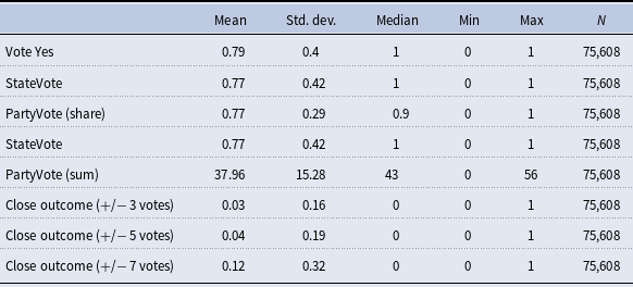
. Table 1 shows summary statistics of the main variables used in the following analysis.
Roll-call voting on state industry issues: description of the main variables

Table 1 Long description
A table with 8 rows and 7 columns summarizing statistics of main variables in U.S. Senate roll-call votes on state industry issues. The columns are labeled Mean, Std. dev., Median, Min, Max, and N. The rows are labeled with different variables: Vote Yes, StateVote, PartyVote (share), StateVote, PartyVote (sum), Close outcome (+/- 3 votes), Close outcome (+/- 5 votes), and Close outcome (+/- 7 votes). Each row provides summary statistics for the respective variable, including the mean, standard deviation, median, minimum, maximum, and the number of observations (N).
This table reports summary statistics of the main variables in our sample of roll-call votes in the U.S. Senate. The sample covers the 20-year period from the 101st to the 110th U.S. Congress. All variables/observations are directly taken from the ready-made original dataset provided by Cohen and Malloy (Reference Cohen and Malloy2014).
We prepare this dataset in order to apply our method as follows. First, based on the information on bill relevance to specific industries, we encode
 $\mathbb{P}$
in line with CM’s underlying theory.
 $\mathbb{P}_{ik}=1$
if a major industry in senator
 $i$
’s state is affected by the bill voted on in roll call
 $k$
and zero otherwise. Second, we estimate different specifications of CM’s baseline linear probability model in order to compute the senators’ propensities to vote Yes and construct
 $\mathbb{Q}$
(see Section 4 for an explanation on
 $\mathbb{Q}$
). Applying the exclusion guideline introduced in Section 3, we control for PartyVote and StateVote—the main observable drivers of expected voting behavior in CM’s setting—but deliberately exclude CM’s main explanatory variable of interest, school-connected votes, because it operationalizes the very trading mechanism we aim to detect and would therefore be absorbed into
 $\mathbb{Q}$
as “expected” voting behavior.Footnote
18
Third, we construct
 $\mathbb{D}$
by identifying Yes votes with a Yes-vote probability below 0.5 that took place in roll calls with narrow outcomes. Table 2 presents the estimation of
 $\mathbb{Q}$
.
Voting on state industry issues in the U.S. Senate

Table 2 Long description
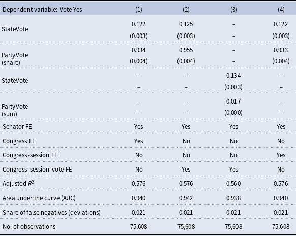
A table with four columns and multiple rows showing regression coefficients for different specifications of a baseline linear probability model. The dependent variable is an indicator equal to 1 if a senator voted Yes. The table includes standard errors clustered at the senator level in parentheses. Row 1: StateVote, 0.122, 0.125, 0.122, (0.003), (0.003), (0.003). Row 2: PartyVote (share), 0.934, 0.955, 0.933, (0.004), (0.004), (0.004). Row 3: StateVote, 0.134, (0.003). Row 4: PartyVote (sum), 0.017, (0.000). The table also includes fixed-effect indicators for Senator FE, Congress FE, Congress-session FE, and Congress-session-vote FE. Additional metrics include Adjusted R-squared, Area under the curve (AUC), Share of false negatives (deviations), and the number of observations, all of which are consistent across the four columns.
This table shows the estimated regression coefficients of different specifications of our baseline linear probability model. The dependent variable is an indicator equal to 1 if a senator voted Yes. Standard errors clustered at the senator level are shown in parentheses.
The estimated regression coefficients are similar to CM’s results, indicating that both StateVote and PartyVote are important predictors of the representatives’ usual voting behavior. In line with their main results, different specifications regarding the granularity of time-fixed effects (congress, session, or vote-specific) change the overall explanatory power of the model only marginally, as the adjusted
 $R^{2}$
s suggest. Similarly, the accuracy of the predictions of Yes/No votes, computed as the area under the ROC curve (AUC), does not vary substantially between the different specifications. The same holds for the share of false negatives (deviations). As the relevant characteristics of the different model specifications do not vary substantially, we use specification 1 to construct
 $\mathbb{Q}$
and
 $\mathbb{D}$
.Footnote
19
For the null model, we construct random networks by generating alternative deviation matrices
 $\mathbb{D}$
from Bernoulli trials of the observed deviations, each one with a probability of success determined by
 $\mathbb{Q}$
. We propagate the uncertainty from the regression estimates to the null model by randomizing the entries in
 $\mathbb{Q}$
according to the standard errors of the predicted probabilities in each entry. First, we create an
 $N \times K$
matrix
 $\mathbb{E}$
where each entry corresponds to the standard errors. In other words, each entry
 $\mathbb{E}_{ik}$
is the standard error of the predicted vote
 $\mathbb{Q}_{ik}$
, given by
 $\mathbb{E}_{ik} = \sqrt {\mathbf{x}_{ik}^{t}\,\mathbb{V}_{\beta }\, \mathbf{x}_{ik}}$
, where
 $\mathbf{x}_{ik}$
is the row of the roll-call-
 $k$
model matrix corresponding to legislator
 $i$
, and
 $\mathbb{V}_{\beta }$
is the variance-covariance matrix of the estimated regression coefficients. These standard errors are used to generate alternative
 $\mathbb{Q}$
s where each entry
 $(i,k)$
is a random draw in the interval
 $[\mathbb{Q}_{ik}-\mathbb{E}_{ik}, \mathbb{Q}_{ik}+\mathbb{E}_{ik}]$
. Each realization of the null model uses one of these randomized
 $\mathbb{Q}$
s.
As part of the null model implementation, alternative mechanisms (unrelated to vote trading) that may generate correlated votes are taken into account in
 $\mathbb{Q}$
(e.g., constituency preferences, sitting next to each other, party, geography, ideology, etc.). That is, the null hypothesis is not responsible for generating alternative DDNs that could emerge from these factors, but rather the method used to construct
 $\mathbb{Q}$
. In practice, the estimation of
 $\mathbb{Q}$
will always be imperfect. However, as we next argue, even if the construction of
 $\mathbb{Q}$
would not fully control for all alternative mechanisms, simple correlations in voting decisions would not constitute a solid alternative to the vote-trading hypothesis. When considering all steps of our approach, any alternative hypothesis aiming to compete with logrolling must explain why it (1) is a deviation, (2) occurs in narrow outcomes, (3) is not accounted for by all the factors explaining usual voting behavior, (4) takes place on bills where someone signaled a strong preference, and (5) is systematically reciprocal. Simultaneously accounting for these features sets a rather high bar when considering alternative mechanisms that may lead to systematically reciprocal deviation patterns.
Finally, to propagate uncertainty to the logrolling index, we construct bootstrap confidence intervals. The procedure consists of resampling (with replacement) the population of legislators in the data. For each resampling, we re-construct all the matrices, re-deploy the null models, and re-compute the logrolling index. The distribution of
 $\ell$
resulting from this procedure provides the basis to construct a confidence interval that can be used to assess if the index is statistically greater than zero, which would provide evidence of significant vote-trading activity. Section C in the appendix provides further details on computing the bootstrap confidence intervals and examines their behavior. The bootstrap intervals converge to the true index as the sample size grows, which is consistent with Monte Carlo confidence intervals that can be estimated through the agent-based model used in the validation section (because with that model one knows the data-generating mechanism).
5.3 Results
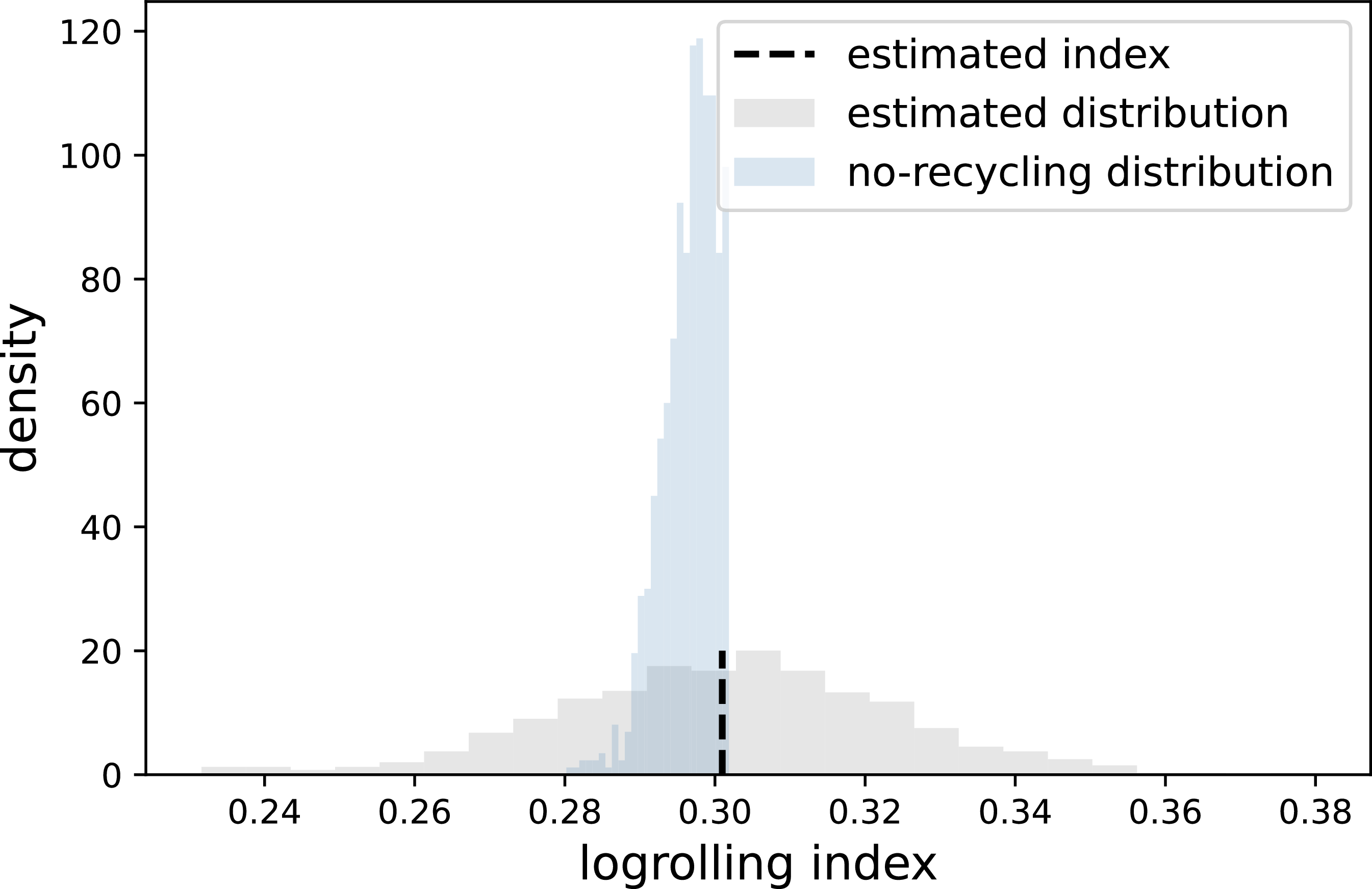
Figure 4 presents the estimated logrolling index and the corresponding bootstrap distribution. As shown by the plot, vote trading is prevalent in the context under study, as the index is approximately 0.3 and its distribution does not contain the zero. In contrast with the case presented in Section 4, CM’s context considers bills with multiple supporters. Therefore, Figure 4 shows the logrolling index assuming that only one supporter is the one potentially engaging in vote trading. We obtain this estimate by generating an alternative matrix
 $\mathbb{P}$
that contains only one supporter (randomly chosen) for each bill. The blue distribution presents the re-estimated logrolling index for a large ensemble of these matrices. We can see that the estimated logrolling index still falls within the distribution of the one-supporter scenario, suggesting that the estimate is robust.
Estimated and corrected logrolling index from the CM data. Distributions generated from 10,000 independent estimations.

These results constitute novel evidence consistent with the theory that senators trade votes on bills that are highly relevant for some states’ major industries. Our findings in this first application suggest that senators exchange favors in the form of vote trading when a bill is particularly relevant for their state’s major industries but irrelevant to the major industries in some of their colleagues’ states.
6. Application II: Trading votes on bill amendments in the U.S. House
The seminal contribution by Stratmann (Reference Stratmann1992) (ST in what follows) tests a logrolling hypothesis on specific votes on five amendments to the Food Security Act of 1985 (i.e., the so-called “Farm Bill” of 1985; H.R. 2100) in the first session of the 99th U.S. House. This is the first quantitative study of vote trading that provides statistical evidence on this type of activity. The study is motivated by qualitative records pointing to the suspicion of vote trading taking place through amendments among specific interest groups.Footnote 20 Using a system of voting regressions at the level of individual legislators’ voting decisions, ST finds statistical evidence of vote trading, considering a reduced number of votes that meet the characteristics of the qualitative reports. Because of the highly contextual knowledge required to identify votes that are susceptible to vote trading, ST’s method cannot be scaled up to estimate the prevalence of vote trading across the entire U.S. House of Representatives.Footnote 21 Therefore, the aim of this application is to estimate the logrolling index in a broader context (still through amendments) and across time in the U.S. House; something that has not been achieved in the literature. Furthermore, we seek to validate ST’s prior on special-interest groups being prone to engage in vote trading.
To consider the broader context, we put forward a generalized vote trading theory that builds on ST’s: representatives with close ties to special interests exchange favors to modify a bill and make it more attractive for all special interests involved in the trade. While ST focuses on reoccurring roll calls that cover agricultural subventions, we expand the sample to all sponsored amendments in the data. Since not every bill is open for amendments, trades between representatives that favor certain amendments might be scarce but recurring The majority leader/speaker of the House controls whether and how amendments are possible when a bill is debated on the floor (via the Rules Committee). Often, the procedural rules are set such that a bill cannot be amended. Such scarcity and recurrence suggest that vote trading via amendments might be particularly prevalent in intermittent (relatively short) periods.
6.1 Data and specification
We collect data on amendment sponsorships by individual representatives as well as the corresponding roll-call records. The roll-call data is obtained from the Office of the Clerk of the U.S. House of Representatives (http://clerk.house.gov). Data on amendment sponsorships is collected from the official bill data published by the Library of Congress (www.congress.gov).Footnote
22
We select a 10-year observation period (97th and the 101th Congress; 1981 to 1990) around the few votes analyzed by ST (votes on the amendments to the 1985 “Farm Bill”). Moreover, we restrict the sample to roll-call outcomes in line with the narrowness criterion applied in ST (
 $\pm 30\%$
). The final dataset consists of roughly 500,000 individual voting decisions in roll calls on bill amendments in the U.S. House. It contains the handful of votes analyzed in ST as well as other cases of votes on bill amendments taking place over the five years prior and posterior to the 1985 “Farm Bill”.Footnote
23
Table B2 in the appendix provides summary statistics of the key variables.
For the econometric model, we use a similar approach as in Section 5.Footnote
24
We model Yes votes as a function of StateVote and PartyVote and include legislator fixed effects and different time-fixed-effect specifications. Consistent with the exclusion guideline in Section 3, we do not include variables that operationalize ST’s amendment-based trading mechanism (amendment-sponsorship alignment between representatives), since these are captured directly by the revealed-preference structure
 $\mathbb{P}$
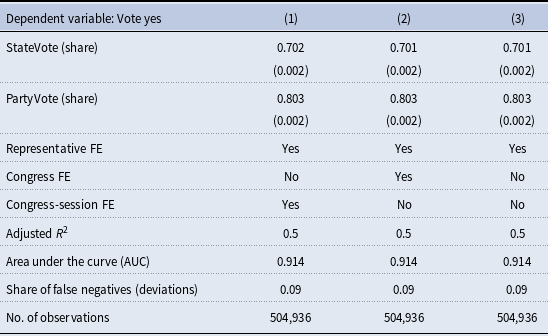
and the reciprocal part of the DDN. Table 3 shows the results of the regression estimates. As in the previous application, a large share of the Yes votes is accurately predicted by these models and, again, the differences between the three alternative specifications with regard to accuracy, predictive power, as well as the resulting share of deviations are minimal. We select specification 3 to compute
 $\mathbb{Q}$
and show that our main results are robust to selecting one of the other specifications (in Section D of the appendix).
Voting on bill amendments in the U.S. House of representatives

Table 3 Long description
The table has 3 columns and 9 rows. Column headers are: Dependent variable: Vote yes, (1), (2), and (3). Row labels are: StateVote (share), PartyVote (share), Representative FE, Congress FE, Congress-session FE, Adjusted R squared, Area under the curve (AUC), Share of false negatives (deviations), and No. of observations. Row 1: StateVote (share), 0.702 (0.002), 0.701 (0.002), 0.701 (0.002). Row 2: PartyVote (share), 0.803 (0.002), 0.803 (0.002), 0.803 (0.002). Row 3: Representative FE, Yes, Yes, Yes. Row 4: Congress FE, No, Yes, No. Row 5: Congress-session FE, Yes, No, No. Row 6: Adjusted R squared, 0.5, 0.5, 0.5. Row 7: Area under the curve (AUC), 0.914, 0.914, 0.914. Row 8: Share of false negatives (deviations), 0.09, 0.09, 0.09. Row 9: No. of observations, 504936, 504936, 504936.
This table shows the estimated regression coefficients of different specifications of our baseline linear probability model, explaining representative’s voting decisions on bill amendments. The dependent variable is an indicator equal to 1 if a representative voted Yes. Standard errors are clustered at the representative level and are shown in parentheses.
In order to provide more nuanced results, we analyze vote trading across time and at different time scales. To achieve this, first, we define a time scale through a window size. Second, we choose an initial point in time and isolate the subsample of consecutive columns in
 $\mathbb{Q}$
,
 $\mathbb{P}$
, and
 $\mathbb{D}$
that fit within the window. Third, we estimate the logrolling index for the subsample. Fourth, we roll the window one period (column) forward in time and repeat the previous steps. We keep rolling the window until the sample period has been covered. The result is the logrolling index across time under the assumption that vote trading occurs in the time span defined by the window. In this application, we focus on window sizes between 2 and 40 roll calls as this is consistent with ST’s vote trading theory on exchanging votes through intermittent amendments not far away from each other.
6.2 Results
Figure 5 shows the (positive) magnitude of the logrolling index across time and window-size specification (periods without a statistically significant index are left blank). First, for smaller window sizes, vote trading through amendments becomes intermittent. This is ST’s context vote-trading theory. Second, the shaded area highlights the roll calls where the votes analyzed in ST took place. Thus, our findings suggest that, during the specific period analyzed in ST, logrolling was likely prevalent, even when the window size is the smallest.Footnote 25
Vote trading in amendments across time. Top panel: average logrolling index across 40 different window sizes. The
 $x$
-axis indicates the initial period of the time window and the Congress number in parenthesis. Bottom panel: positive and significant (at 95%) logrolling indices across the different combinations of initial periods and window sizes. One point in the top panel is computed through the average across rows in the bottom panel (in the same column). The shaded area corresponds to ST’s sample period. The results received the effective-n Bonferroni correction that divides the level of statistical significance (5%) by the ratio of number of bills to the window size of each row in the bottom panel. Hence, the “wholes” in the bottom panel denote false positives that the correction removes. according to the window size and the number of bills.

In a second step, we explore whether the bill amendments voted on in reciprocal deviations tend to be related to special interest politics (both in general as well as specifically for ST’s case of agriculture), as ST’s vote-trading theory suggests. We extend our roll-call dataset with the policy issue categories developed by Peltzman (Reference Peltzman1984) and the issue categorization by Clausen (Reference Clausen1973). With this additional information, we can distinguish four types of roll-calls that are relevant in ST’s hypothesis: votes on issues explicitly related to special interests (Special Interest), votes on issues explicitly related to special interests in the domain of agriculture (Special Interest: Agriculture; nested in Special Interest), votes on issues explicitly related to general interests/the public (General Interest), and all votes not explicitly related to special interests (Other; nests General Interest).Footnote 26
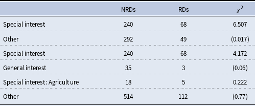
We perform chi-squared tests of independence to assess whether the votes captured in the reciprocal part of the DDN are, overall, systematically more likely to fall into the special interest categories outlined above in comparison to those votes not involved in reciprocal deviations.Footnote 27 Table 4 shows the results.
Frequency counts and
 $\chi ^{2}$
-tests of special interest reciprocal deviations

Table 4 Long description
A table with four rows and three columns comparing frequency counts and chi-squared tests of special interest reciprocal deviations. The columns are labeled NRDs, RDs, and χ². The row labels are Special interest, Other, Special interest, and General interest. Row 1: Special interest, 240, 68, 6.507. Row 2: Other, 292, 49, (0.017). Row 3: Special interest, 240, 68, 4.172. Row 4: General interest, 35, 3, (0.06). Row 5: Special interest: Agriculture, 18, 5, 0.222. Row 6: Other, 514, 112, (0.77). The table shows frequency counts of votes on special interest issues vs non-special interest issues, occurring or not occurring in the reciprocal part of the DDNs. The right-most column presents chi-squared statistics of a test of independence based on the corresponding frequency counts (p-values based on 2,000 bootstrap trials shown in parentheses).
This table shows frequency counts of votes on special interest issues vs non-special interest issues (following Clausen, Reference Clausen1973 and Peltzman, Reference Peltzman1984), occurring or not occurring in the reciprocal part of the DDNs underlying Figure 5. The right-most column presents chi-squared statistics of a test of independence based on the corresponding frequency counts (p-values based on 2,000 bootstrap trials shown in parentheses). NRDs: not reciprocal deviations. RDs: reciprocal deviations.
The results indicate an over-proportional representation of special interest-related amendment votes captured by the reciprocal part of the DDN (when comparing special interest-related issues with all other types of votes). The same picture holds for a comparison with votes explicitly related to general interest policies. However, there is no over-representation of votes related to special interest politics in the domain of agriculture captured by the reciprocal part of the DDN. In sum, our findings are consistent with the generalization of ST’s theory that representatives engage in logrolling when voting on bill amendments related to special interest politics, but cannot confirm whether these types of trades occur in the specific context of agricultural policies, at least not exclusively through amendments.
7. Discussion and conclusions
While broadly covered in the theoretical literature, little is known about the prevalence, variability, and underlying mechanisms of legislative vote trading in the real world. One key challenge for empirical research on the topic is the hidden nature of vote trading. Our approach can be used to find reciprocal voting patterns consistent with specific theories of vote trading, integrating and complementing existing approaches. Our method might therefore allow a broader empirical assessment and understanding of this form of hidden cooperation in politics.
Following the core assumptions about the incentives to trade votes underlying previous empirical contributions (Cohen and Malloy, Reference Cohen and Malloy2014; Stratmann, Reference Stratmann1992, Reference Stratmann1995), our approach builds on three theoretical pillars, characterizing the minimal requirements to consider an observed vote as traded. These pillars are integrated at the heart of the empirical approach and allow combining our framework with econometric approaches. By building on the concept of reciprocity in directed, weighted networks, we can incorporate the micro-structure of reciprocal deviations between individual members of a legislature into a measure for the prevalence of vote trading in roll-call data. As the suggested logrolling index is built from the bottom up, it is straightforward to explore how the statistical evidence of vote trading has emerged based on the underlying individual voting behavior.
Our framework, like the previous ones, has important limitations. It is critical to keep in mind that there might be other forms of vote trading that are not captured by our approach. Two aspects are of particular relevance. First, the two applications of our method (amendment-sponsorships and favored state-specific industrial policies) are, of course, not the only perceivable indication of strong preferences toward bills. As in the previous contributions on which we build these applications, alternative observable indications for policy preferences might also reveal tendencies to trade votes. In such cases, there might be a need for alternative models/methods (and/or controls) to estimate
 $\mathbb{Q}$
as well as a potential adaptation of the DDN null model. Second, it might be that some deals are arranged between groups. In those cases, our method would likely capture the roll calls/bills affected by such trades, but not each individual participating in the deal. This also opens our (and the previous approaches in the literature) to the problem of how we can get and integrate more prior knowledge about which legislators should be considered potential trading partners. By default, the method allows trades between any two legislators in a legislature. Prior knowledge about the specific legislative setting can be incorporated to reduce the number of potential trading partners. A key challenge in this context is the scalability of prior knowledge about potential trades (potential trading partners). We consider this a key area for future research on legislative vote trading and the development of empirical methods to study vote trading.
Related to the previous points, researchers using our method have to carefully contextualize its application. That is to say, comparability of the logrolling index over time and/or across different legislatures hinges on careful tailoring of (i) what counts as a “deviation” and (ii) the null model to each institutional context. When those design choices are justified consistently, the index can be compared across chambers or periods; when they are not, such comparisons would be inappropriate.
Finally, our method can only assess the potential prevalence of trades based on pairs of legislators and not more complex trade constructs such as triads. However, we still consider the exclusive focus on underlying pairwise trades substantially better than not considering reciprocity at all when studying a specific setting of vote trading.
In conclusion, the proposed framework can serve as a valuable tool for future research on vote trading. Taking the important limitations into account, its flexibility and scalability can aid in the discovery and study of vote trading at various levels of government, across time, as well as across different jurisdictions and institutional settings.
Acknowledgements
We thank Patrick Balles, Irene Dávalos, Ben Golub, Bernard Grofman, Roland Hodler, Yarden Katz, Jeffrey Lienert, Eduardo Lopez, Dietmar Maringer, Armando Meier, Reto Odermatt, Sanna Ojanperä, David Parkes, Dennis Quinn, Felix Reed-Tsochas, Matteo Richiardi, Serguei Saavedra, Kurt Schmidheiny, Nicolas Schreiner, Kenneth Shepsle, Michaela Slotwinski, Alois Stutzer. O.A.G. acknowledges the financial support of the Institute for New Economic Thinking at the Oxford Martin School through the grant INET12-9001 and the EPSRC grant EP/N510129/1. U.M. acknowledges a seed grant provided by the University of Basel Research Fund as well as support from the Swiss National Science Foundation (grant 168848).
Supplementary material
The supplementary material for this article can be found at https://doi.org/10.1017/nws.2026.10048.
Competing interests
The authors declare no competing interests.





 x
 χ2


 Open access

