1. Background

As high-performance computing initiatives bring the advent of the exascale era, numerical simulations become capable of providing prediction with high levels of accuracy. In toroidal magnetic confinement fusion devices, the hot plasma dynamics is determined by space–time overlapping multiscale interactions among complex multiscale physics. Calculating these interactions is computationally expensive, especially in the case of total-f gyrokinetic codes, which solve for the motion of particles on turbulence scales and the background scale together without scale separation. XGC (X-point Gyrokinetic Code) is a massively parallel hybrid Lagrangian–Eulerian particle-in-cell-based gyrokinetic code focused on simulating the highly nonlinear, non-equilibrium edge region of fusion devices (Ku et al. Reference Ku, Chang, Hager, Churchill, Tynan, Cziegler, Greenwald, Hughes, Parker and Adams2018). An expensive part of the code is the collision operator acting on the five-dimensional particle distribution functions. XGC uses the nonlinear Fokker–Planck–Landau (FPL) collision operator (Landau Reference Landau1936), seen in (1.1), on a two-dimensional normalized velocity grid, $v_\perp /v_{\textrm {th}},v_\parallel /v_{\textrm {th}}$ (spatial points are independent in the collision operator) (Yoon & Chang Reference Yoon and Chang2014; Hager et al. Reference Hager, Yoon, Ku, D'Azevedo, Worley and Chang2016). At every time step, particles tracked in three-dimensional configuration space and two-dimensional velocity coordinates are histogrammed into velocity particle distribution functions $f$ on regular, two-dimensional velocity grids at each configuration space vertex. An implicit Picard iteration scheme is then used to solve the integro-differential equation involving the collision operator on the two-dimensional velocity grid at each configuration space vertex, with a typical number of configuration space vertices in a simulation of the order of $10^1$–$10^2$ million:

(1.1)\begin{equation} \frac{\textrm{d}f_a}{\textrm{d}t} = \sum_b C_{ab}(\,f_a;f_b') ={-}\sum_b \frac{e_a^2e_b^2ln\varLambda_{ab}}{8{\rm \pi}\epsilon_0^2m_a} \boldsymbol{\nabla}_v \boldsymbol{\cdot} \int \boldsymbol{\mathsf{U}} \boldsymbol{\cdot} \left(\frac{f_a}{m_b} \boldsymbol{\nabla}_v' \,f_b' - \frac{f_b'}{m_a} \boldsymbol{\nabla}_v \,f_a\right)\,\textrm{d}^3v'. \end{equation}

In (1.1), $a$ and $b$ denote separate species, although self-collisions are included in the case that $b = a$. Functions $f_a$ and $f_b$ are the particle distribution functions of the species, $e_{a,b}$ is the charge, $m_{a,b}$ is the mass, $\ln \varLambda _{ab}$ is the Coulomb logarithm and $\boldsymbol{\mathsf{U}}$ is a tensor that is a function of the relative vector $\boldsymbol {u} = \boldsymbol {v} - \boldsymbol {v'}$:

(1.2)\begin{equation} \boldsymbol{\mathsf{U}} = \frac{u^{2}\boldsymbol{I} - \boldsymbol{u}\boldsymbol{u}}{u^{3}}. \end{equation}

The run time for the Picard iteration solver of the collision operator in XGC1 for production runs with electrons turned on is currently $\sim 10\,\%$ of the overall compute time. This number increases in higher-collisionality regimes. The run time for the operator, however, is $O(n^2)$, where $n$ is the number of plasma species. As the XGC1 code begins to attack problems including a larger number of species, such as including impurities like tungsten and its multiple charge states in devices like ITER, the collision operator will become the dominant computation (Dominski et al. Reference Dominski, Chang, Hager, Helander, Ku and Yoon2019).

Deep neural networks have proven successful for many computer vision tasks, including image recognition, as well as text and speech recognition. Given their success, a great deal of effort has been expended in utilizing them to solve complex problems across science and engineering. Specifically in physics, their application is widespread. From learning field theories using a set of training data produced from a physical field (Qin Reference Qin2019), to simulating particles using a graph network by combining an ordinary differential equation integrator with Hamiltonian dynamics (Sanchez-Gonzalez et al. Reference Sanchez-Gonzalez, Bapst, Cranmer and Battaglia2019), to predicting nonlinear, cosmological large-scale structures of the universe (He et al. Reference He, Li, Feng, Ho, Ravanbakhsh, Chen and Póczos2019), neural networks have proven extremely versatile.

Recognizing the importance of efficient partial differential equation (PDE) solvers across the field of physics, a more concerted effort is underway to use neural networks to help solve especially intractable PDEs. Almost always, training of a PDE solver using neural networks depends on minimizing an objective function that is composed primarily of the quadratic residual, also known as mean-squared error or $\ell _2$ loss. Consider a stationary PDE of the form

(1.3)\begin{equation} \left. \begin{gathered} Lu = f, x\in\varOmega,\\ Bu = g, x\in\varGamma\subset\partial\varOmega, \end{gathered} \right\} \end{equation}

where $L$ is a differential operator, $f$ is a forcing function, $B$ is a boundary operator and $g$ are boundary data. Solutions then require the minimization of an objective function composed of the $\ell _2$ loss as follows:

(1.4)\begin{equation} C = \alpha ||L\hat{u} - f||^{2}, \end{equation}

where $\hat {u} = \hat {u}(\theta ,\phi ,\ldots )$ is the ansatz that depends on some number of trainable parameters $\theta$, $\phi$, etc. that can be optimized to minimize (1.4). Here $\alpha$ is some coefficient that can vary and that becomes especially important as other terms are added to the objective function.

While this methodology is common to PDE neural network techniques, the incorporation of boundary conditions, or any constraints in general, varies. Often, these constraints are built into the network itself as ‘hard’ constraints, either directly into the architecture or into a constraint on the ansatz. Some methods attempt to do the former by adding a differentiable PDE layer that enforces spatial constraints (Jiang et al. Reference Jiang, Marcus, Kashinath and Marcus2020) or in the case of a simple governing PDE, the use of an untrainable ‘physics embedded decoder’ that replicates the differential operator and boundary conditions directly (Mohan et al. Reference Mohan, Lubbers, Livescu and Chertkov2017). Others use the boundary conditions to constrain the ansatz itself and then proceed with unconstrained optimization of an objective function like in (1.4) (Berg & Nyström Reference Berg and Nyström2018). One last set of techniques treats the constraints as ‘soft’ and instead incorporates them into the objective function as penalty terms. This is done by adding the boundary conditions directly into the loss function (Sirignano & Spiliopoulos Reference Sirignano and Spiliopoulos2018) or by leveraging the use of a coefficient like $\alpha$ in (1.4) that allows for a relative prioritization of different constraints in the loss function (Beucler et al. Reference Beucler, Pritchard, Rasp, Ott, Baldi and Gentine2019).

This paper employs a technique very similar to the latter. Using a penalization method to optimize ‘soft’ constraints, it aims to learn the nonlinear transformation of the collision operator in (1.1), enabling the XGC code to be accelerated. Since the FPL collision operator can be expressed as solving the collisional change $\Delta f_a = F(\,f_a,f_b,\ldots )$, where $\Delta f_a$ is the same size on the normalized two-dimensional velocity grid as $f_a$, $f_b$, etc. in a non-equilibrium edge plasma, here we use encoder–decoder deep neural networks used in the common computer vision task of semantic segmentation.

2. Machine learning in computer vision

Computer vision has been one of the largest drivers for machine learning algorithm development. During the ImageNet competition, it was quickly noticed that deep convolutional neural networks (CNNs) performed best for image recognition (Alom et al. Reference Alom, Taha, Yakopcic, Westberg, Nasrin and Asari2018). These networks take in an input image and output a set of scores corresponding to a set of possible categories that identify the image. The largest of these scores corresponds to the prediction of the network. Structurally, the input has dimensions $H \times W \times 3$, where $H$ is the number of image pixels vertically, $W$ is the same horizontally and 3 corresponds to the three colour channels, red, green and blue. The output is simply a one-dimensional vector with $C$ elements, where $C$ is the prescribed number of possible identification classes. A CNN contains a variable number of hidden layers which perform convolutions on the input image in an attempt to discern underlying features to aid in identification. At each of these layers, a convolution kernel performs a convolution, or formally a cross-correlation, on the data. For neural networks, this is performed in two dimensions as follows (although the operation generalizes to higher dimensions):

(2.1)\begin{equation} (\,f*g)(i,j) = \sum_{m=0}^{M} \sum_{n=0}^{N} f(m,n)g(i+m,j+n), \end{equation}

where $f$ is the input into the convolution layer $g$. For a function represented by a matrix, as is the case for neural networks, $m$ and $n$ simply iterate over the two dimensions of the matrix, $M$ and $N$, respectively, and $i$ and $j$ are used to index a particular element of the convolution (Kao Reference Kao2017).

Along with these convolutional layers, the data are passed through a nonlinear activation function at each layer, allowing the network the flexibility to learn the nonlinearities associated with many real-world problems. Every few convolutions, the data are passed through a learned filter that ‘summarizes’ the features in the input image. These layers, called pooling layers, reduce the number of parameters in the network. Finally, the CNN ends with a set of fully connected layers that terminate with a linear operation that transforms the final two-dimensional feature map into a vector containing the $C$ class scores. As with any gradient-based optimization problem, a loss function allows for computation of gradients and updating of the weights of the network to attempt to minimize the loss (Kao Reference Kao2017).

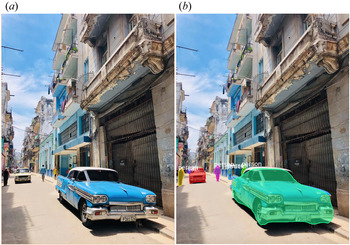
As computer vision networks increased in sophistication, they turned to more complicated tasks like that of semantic segmentation. This involves classifying each pixel in an image, allowing the network to identify every part of an image. An example of an image parsed by a neural network with this goal is shown in figure 1. This framework of making pixel-wise decisions on a input dataset is of great use to a variety of unrelated problems, in particular to accelerating solutions to the equations governing the collision of particles in a tokamak. To understand why, it is necessary once again to consider the spatial arrangement of data that semantic segmentation techniques manipulate.

Figure 1.

Example image of semantic segmentation being used to identify all cars and people in an image. Each object in (b) corresponds to a class prediction by the neural network, for the input image in (a). (Original photograph courtesy of A. Gnaedinger.)

Semantic segmentation is the computer vision task of labelling each pixel with the object class to which that pixel belongs, e.g. marking all pixels that belong to a car in an image. For semantic segmentation, the input is an image of dimensions $H \times W \times 3$. As each pixel receives a class score, the output takes the form $H \times W \times C$. Since the image has $H \times W$ pixels, the output array must contain $H \times W$ vectors of $C$ elements. To do this, the network ‘encodes’ the input image by down-sampling it into a series of arrays that abstracts the features of an image, before ‘decoding’ these features by up-sampling these feature maps back into a an array of dimensions $H \times W \times C$. The classification of a certain object is now made at a pixel level, $H \times W$ times. For each of these pixels, there is an associated cross-entropy loss function from which the total overall loss is computed, which is then used in backpropagation to update the overall gradients.

3. Computer vision technique for collision operator

Semantic segmentation techniques are a good starting point for attacking the collision operator prediction problem, specifically because of the similarities between the hierarchies of convolutions in CNNs and the velocity-space gradients in the FPL collision operator. Numerical gradients involve a local finite difference stencil to calculate derivatives, which CNNs can naturally mimic and learn optimal weights for, as the convolutions are local two-dimensional grid operations. To perform the collision calculation, at every time step, XGC performs particle to mesh interpolation, creating distribution functions on regular two-dimensional velocity grids of size $N_{v_{\textrm {perp}}} \times N_{v_{\textrm {par}}}$ at each configuration grid vertex. This array can be thought of as a set of bins representing the number of particles at particular velocities, both parallel and perpendicular to the magnetic field lines.

XGC creates distribution functions on each mesh vertex for each particle type simulated. In this case, we consider electrons and a single ion species. The collision operator takes in these distribution functions and performs the collision calculation according to the FPL equations and outputs the change in the distribution function of species $a$, labelled $\Delta f_{a,\textrm {col}}$. For example, the ion $\Delta f_{i,\textrm {col}}$ is

(3.1)\begin{equation} \Delta f_{i,\textrm{col}} = \Delta t \boldsymbol{\cdot} C_i(\,f_i,f_e) = \Delta t \boldsymbol{\cdot} \left[ C_{ii}(\,f_i,f_i) + C_{ie}(\,f_i,f_e) \right], \end{equation}

where $\Delta t$ is the XGC ion time-step size. This $\Delta f_{a,\textrm {col}}$ has the same configuration space size as the original distribution function, much like semantic segmentation techniques which preserve, the size of an input image.

One main difference between the collision operator and typical semantic segmentation is that $\Delta f_{a,\textrm {col}}$ is continuous, such that it is a regression problem instead of a classification problem. We use a mean-squared error loss (or $\ell _2$) as part of the loss function:

(3.2)\begin{equation} L_{\ell_2} = \frac{1}{N} \sum_{i=1}^N (\Delta f_{\textrm{XGC}} - \Delta f_{\textrm{ML}})^2 , \end{equation}

where $N$ is the number of configuration space vertices, $\Delta f_{\textrm {XGC}}$ is the result of the typical Picard iteration solver used by XGC and $\Delta f_{\textrm {ML}}$ is the predicted $\Delta f$ from the machine learning neural network. Given that this is the only difference from semantic segmentation frameworks, networks that have proven successful in this area can be directly used to predict the outputs of the Picard iteration solver, with a minor adjustment to the final layers of the network (detailed at the end of § 5) and a loss function appropriate to this problem.

4. Physics-inspired constrained learning

In a general regression problem, the $\ell _2$ loss is sufficient to train a network to minimize the loss of a nonlinear transformation. In this problem, however, we are dealing with a physical system that is constrained by physical laws, namely the laws of particle density, momentum and energy conservation. The $\ell _2$ loss does not directly take into consideration the conservation laws of the collision operator and is often insufficient to ensure these physical constraints are satisfied. For two species, $a$ and $b$, the conservation equations can be summarized as follows (Helander & Sigman Reference Helander and Sigman2002):

(4.1)\begin{equation} \int \phi_a(\boldsymbol{v}) C_{ab}(\,f_a,f_b) \, \textrm{d}^3v ={-}\int \phi_b(\boldsymbol{v}) C_{ba}(\,f_b,f_a) \, \textrm{d}^3v, \end{equation}

where $\phi (\boldsymbol {v}) = \{1,m\boldsymbol {v}, (m v^2)/2\}$ represent particle density, momentum and kinetic energy.

For particle density conservation it can be shown more specifically that

(4.2)\begin{equation} \int C_{ab}(\,f_a,f_b) \, \textrm{d}^3v = 0. \end{equation}

Note also that for self-collisions, $a=b$, equation (4.1) reduces further:

(4.3)\begin{equation} \int \phi_a(\boldsymbol{v}) C_{aa}(\,f_a,f_a') \, \textrm{d}^3v = 0. \end{equation}

4.1. XGC implementation

Details of the FPL collision operator can be found in Yoon & Chang (Reference Yoon and Chang2014) and Hager et al. (Reference Hager, Yoon, Ku, D'Azevedo, Worley and Chang2016). We list here mathematically the conservation properties that XGC uses in the code. For now, we will present continuous, analytical equations and not the detailed numerical implementations (see Hager et al. Reference Hager, Yoon, Ku, D'Azevedo, Worley and Chang2016). Also, we will retain the full 3D–3V notation from § 1, even though XGC is gyrokinetic (3D–2V), and there are a number of differences, but this will suffice to illustrate the main points. We drop the explicit notation inputting the distribution functions into the collision operator ($C_{ab}$), as it is redundant with the subscripts of the collision operator. For simplicity we limit ourselves to the two-species case, electrons (‘$e$’) and a single ion species (‘$i$’).

We use the following moment definitions:

(4.4)\begin{equation} \left. \begin{gathered} n_a = \int f_a \,\textrm{d}^3v, \\ P_a = \int m_a \boldsymbol{v} f_a \,\textrm{d}^3v, \\ E_a = \int \frac{1}{2}m_a v^2 f_a \,\textrm{d}^3v. \end{gathered} \right\} \end{equation}

The conservation properties calculated in XGC are as follows:

(4.5)\begin{equation} \left. \begin{gathered} \Delta n_i = \textrm{d}t \left[\int C_{ii} \, \textrm{d}^3v + \int C_{ie} \, \textrm{d}^3v \right] = 0,\\ \Delta n_e = \textrm{d}t \left[\int C_{ee} \, \textrm{d}^3v + \int C_{ei} \, \textrm{d}^3v \right] = 0,\\ \Delta P_i = \textrm{d}t \left[\int m_i \boldsymbol{v} C_{ii} \, \textrm{d}^3v + \int m_i \boldsymbol{v} C_{ie} \, \textrm{d}^3v \right],\\ \Delta P_e = \textrm{d}t \left[\int m_e \boldsymbol{v} C_{ee} \, \textrm{d}^3v + \int m_e \boldsymbol{v} C_{ei} \, \textrm{d}^3v \right],\\ \Delta E_i = \textrm{d}t \left[\int \frac{1}{2} m_i v^2 C_{ii} \, \textrm{d}^3v + \int \frac{1}{2} m_i v^2 C_{ie} \, \textrm{d}^3v \right],\\ \Delta E_e = \textrm{d}t \left[\int \frac{1}{2} m_e v^2 C_{ee} \, \textrm{d}^3v + \int \frac{1}{2} m_e v^2 C_{ei} \, \textrm{d}^3v \right]. \end{gathered} \right\} \end{equation}

These are combined to form the conservation laws (see (4.1) and (4.5)):

(4.6)\begin{equation} \left. \begin{gathered} \Delta n_i = 0, \\ \Delta n_e = 0, \\ \Delta P = \Delta P_i + \Delta P_e = 0, \\ \Delta E = \Delta E_i + \Delta E_e = 0. \end{gathered} \right\} \end{equation}

Since these are numerical solutions, the terms in (4.6) will not be exactly 0. The quantities in (4.6) when normalized provide a test to determine how close the numerical solver is to satisfying these physical conservation properties. Equation (4.7) gives the conditions for the normalized quantities to satisfy for the algorithm to be considered converged in XGC's numerical Fokker–Planck solver:

(4.7)\begin{equation} \text{converged if} \begin{cases} \left| \dfrac{\Delta n_i}{n_i} \right| & < 10^{{-}10},\\ \left| \dfrac{\Delta n_e}{n_e} \right| & < 10^{{-}10}, \\ \dfrac{|\Delta P_i + \Delta P_e|}{| n_i m_i v_{\textrm{th},i}| + | n_e m_e v_{\textrm{th},e} |} & < 10^{{-}7}, \\ \dfrac{|\Delta E_i + \Delta E_e|}{| E_i + E_e |} & < 10^{{-}7}, \end{cases}\end{equation}

where $v_{\textrm {th},i}$ and $v_{\textrm {th},e}$ are local-average ion and electron thermal speeds, $v_{\textrm {th}} = \sqrt {T/m}$. The average electron momentum is usually negligible compared to the ion momentum. The numerical precision enforced by these criteria at each XGC ion time step is such that the accumulated error throughout the entirety of the XGC simulation is kept below an overall simulation threshold value. The criteria, however, as they are written in (4.7), are overly stringent, and can be relaxed to up to $10^{-6}$ without sacrificing the accuracy of the overall simulation.

4.2. Machine learning implementation

We enforce these physical conservation constraints in our neural network by including them as regularization terms in the loss:

(4.8)\begin{equation} L_{\textrm{cons}} = \sum_{j=1}^3 \lambda_j \sum_{a = \{i,e\}} \frac{\langle \phi_a^j \, \Delta f_{a,\textrm{ML}} \rangle}{A_j}. \end{equation}

This equation incorporates (4.1) into the loss, seeking to minimize the change in these quantities due to the collision operator. Here, $\phi _a^j = \{1,m_a \boldsymbol {v}, (m_a v^2)/2 \}$ and $A_j = \{ n_{i}, | n_i m_i v_{\textrm {th},i}| + | n_e m_ev_{\textrm {th},e} |, | E_i + E_e | \}$ (as in (4.7)) for ion particle density $=$ electron particle density, momentum and energy conservation, and $\langle \rangle$ represents the numerical velocity integral. The quantity $\lambda _j$ represents a hyperparameter scaling factor that allows for modification of how heavily each conservation property is weighed in the overall loss function. This in turn affects how much the network corrects for each of the conservation errors compared to the $\ell _2$ loss. Training results are rather sensitive to changes in these $\lambda _j$. For values too high, the conservation loss decreases too quickly and then plateaus. For values too low, the $\ell _2$ loss dominates optimization. As a result, tuning of these hyperparameters (in conjunction with the learning rate) allowed determination of the optimal values of $\lambda _j$. More sophisticated optimization schemes have been since been implemented. In particular, using an augmented Lagrangian method dynamically updates these hyperparameters, which lessens the burden of manually picking the $\lambda _j$ (Dener et al. Reference Dener, Miller, Churchill, Munson and Chang2020). The overall loss function is simply the sum of $L_{\ell _2}$ (equation (3.2)) and $L_{\textrm {cons}}$ (equation (4.8)).

5. Training set-up and architecture

A dataset of the particle distribution functions $f_i$ and $f_e$ was gathered from XGC, and collision kernel output $\Delta f$ of the existing Picard iteration scheme was generated. These comprised over 2.5 million samples of the $N_{v_\perp } \times N_{v_\parallel } = 32 \times 31$ velocity-space grid distribution functions in the present problem. The data were gathered from a single XGC simulation of shot 79688 of the JET tokamak. The range of the effective collision frequency of the points used is $10^{-2} < \nu ^* < 10$, where $\nu ^*$ is defined as $\nu ^* = ({\nu / \varepsilon ^{3/2}})/({v_{\textrm {th}} / q R})$, where $R$ is the major radius of the machine, $\varepsilon = a/R$ is the inverse aspect ratio and $q$ is the safety factor. The plasma parameters range from electron density $~9\times 10^{19} \ \textrm {m}^{-3}$ in the core to $1 \times 10^{19} \ \textrm {m}^{-3}$ in the near scrape-off layer, and temperature $5\ \textrm {keV}$ in the core to 100 eV in the near scrape-off layer (for this discharge $T_e \approx T_i$). It may eventually be important to ensure the data span a broad enough range of relevant physical parameters. Using the distribution function for both the ions and the electrons allows for calculation of the actual $\Delta f$ within the XGC collision kernel. 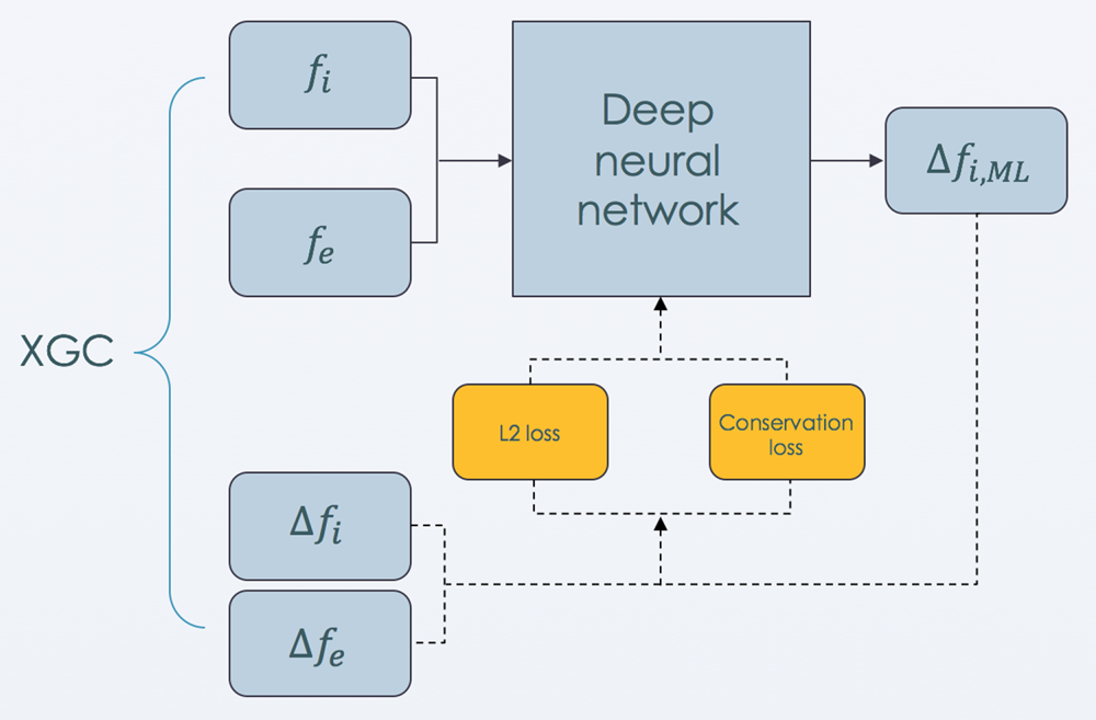The three sets of data, $f_i$, $f_e$ and $\Delta f_i$, can then be used for training the neural network according to the schematic depicted in figure 2. Work is now underway to include $\Delta f_e$ in the training itself, rather than simply using the output $\Delta f_e$ from XGC's collision kernel.

Figure 2.

Schematic of the training processes used for collision prediction.

Before training begins, a few steps are taken to preprocess the data. In the interest of reducing the training time, the training is limited to four toroidal planes. The data from these planes are filtered further to remove points that have non-physical $f$ data and that have target $\Delta f$ that did not converge when passed into the XGC collision kernel. Here, non-physical $f$ implies removing points that have negative values and unconverged points are points that have surpassed the imposed allowed number of iterations in the collision kernel. Once this filtering is done, the entire dataset is divided into three groups: training, validation and testing, comprising 80 %, 10 % and 10 % of the data, respectively. The training data are then split into equal-sized batches before being passed into the neural network.

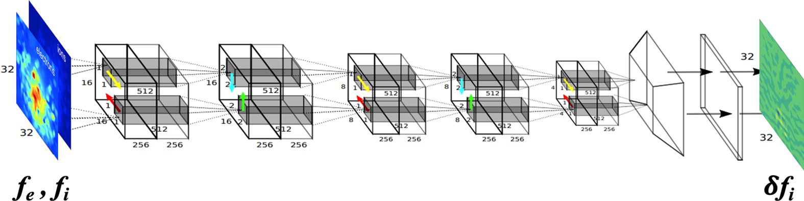
Initial training was begun on U-Net (Ronneberger, Fischer & Brox Reference Ronneberger, Fischer and Brox2015), one of the encoder–decoder networks that performed best on semantic segmentation techniques earlier on. Once initial results were satisfactory, more sophisticated encoder–decoder networks were investigated. In the end, the ReSeg network was chosen, with only a modification to the fully connected linear layer to account for the nature of the problem as regression, not classification (explained in § 3). ReSeg combines CNNs and recurrent neural networks (RNNs) to perform semantic segmentation (Visin et al. Reference Visin, Romero, Cho, Matteucci, Ciccone, Kastner, Bengio and Courville2016). ReSeg begins with a CNN, in this case VGG16 (Simonyan & Zisserman Reference Simonyan and Zisserman2015), which is the encoder for this network (see § 2). This CNN downsamples the input distribution function, producing a grid that is 256 planes deep. ReSeg then stacks two layers of ReNet, each of which is composed of four RNNs that ingest the feature maps sequentially. The decoder consists of two transposed convolution layers, interspersed with ReLU activations, which upsamples the data to a $32 \times 31 \times 100$ grid. For the purposes of this problem, the last layer of the network includes a convolutional kernel of size $1 \times 1 \times 100$ with stride 1, which outputs the desired $32 \times 31 \times 1$ distribution function representing $\Delta f$. For this problem, there are over 2.6 million parameters in the network.

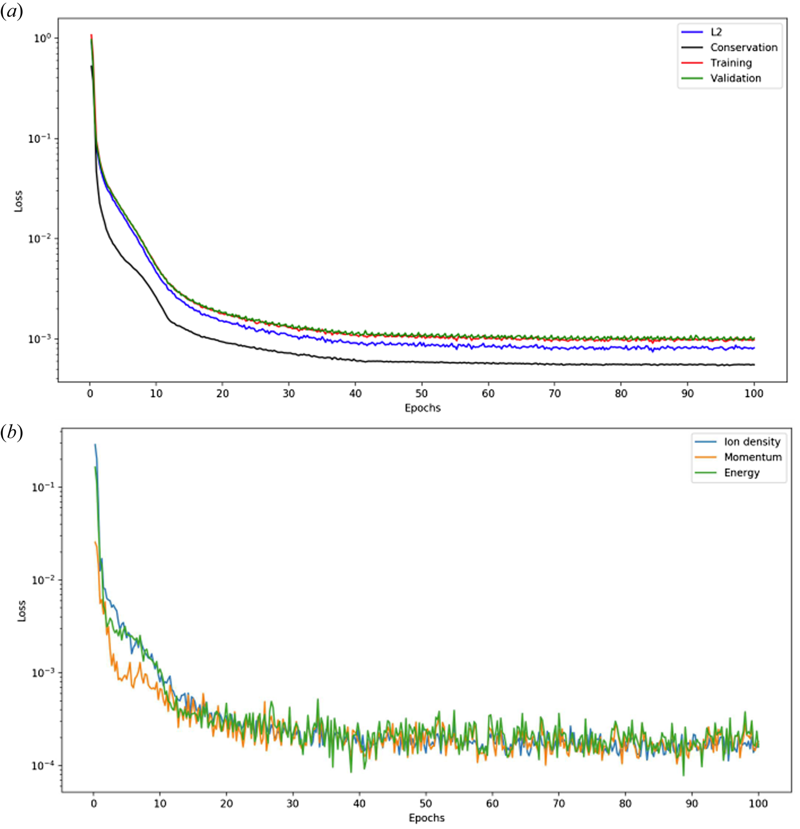
A schematic of the network architecture can be seen in figure 3. Stochastic gradient descent with momentum was used primarily as the optimizer, though RAdam, a variant of Adam that reduces the variance of adaptive learning rates (Liu et al. Reference Liu, Jiang, He, Chen, Liu, Gao and Han2019), also showed success. Training was done for 100 epochs, with a validation set done twice an epoch. The training and validation results are shown in figure 4, with the $\ell _2$ and conservation error shown separately.

Figure 3.

Schematic of ReSeg, a neural network architecture used for semantic segmentation, showing an example input $f_e, f_i$ and output $\delta f_i$. The inputs $f_e$ and $f_i$ are concatenated to form a tensor of depth 2.

Figure 4.

Training results on JET data for 100 epochs and four toroidal planes showing $(a)$ overall training and validation, as well as $\ell _2$ and conservation loss, and $(b)$ the three components of the conservation loss separately.

6. Initial training and validation

Figure 4 shows the training loss over time for 100 epochs of ReSeg training. The learning rate was adjusted using a combination of warm-up and manual learning rate decay every 10 epochs. Note that the ‘training’ and ‘validation’ plots include the $\lambda _j$ from (4.8), while the ‘conservation’ plot does not. It is clear that after around 70 epochs, the loss begins to plateau and learning stagnates. 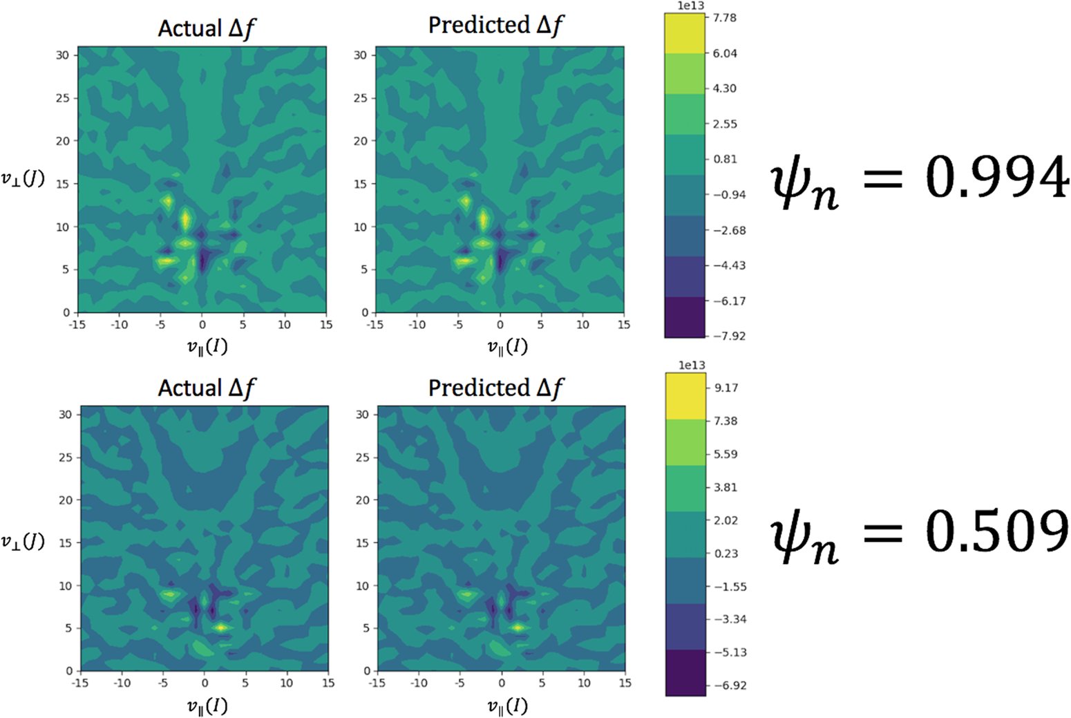This begs a finer tuning of the hyperparameters, or perhaps a revision of the optimization procedure, specifically in the weights assigned to each quantity in the loss function ($\lambda _j$ in (4.8)). Figure 4(b) breaks up the conservation loss into each of three conservation properties: ion particle density, momentum and energy, the three elements of the summation in (4.8). Finally, figure 5 illustrates the difference in learning of the structure of $\Delta f$ for two different $\psi _n$, a normalized radial coordinate, which lie in two different regimes of collisionality. The lower the $\psi _n$, meaning the closer the plasma is to the core, the more Maxwellian the plasma, and so the smaller the resulting $\Delta f$ from the collision operator. Collisions here result in a smaller $\Delta f_{\textrm {col}}$, perhaps making the transformation easier for the network to learn.

Figure 5.

Comparison of $\Delta f_{\textrm {col}}$ prediction in two different regimes of collisionality. The $x$ and $y$ axes represent bins in velocity space (parallel and perpendicular, respectively). The index $I$, representing $v_\parallel$, ranges from $[-15, 15]$, totalling 31 bins in the parallel direction, and the index $J$, representing $v_\perp$, ranges from [0, 31], totalling 32 bins in the perpendicular direction. Plotted $\Delta f_{\textrm {col}}$ actually includes a volume factor related to XGC normalizations not removed here.

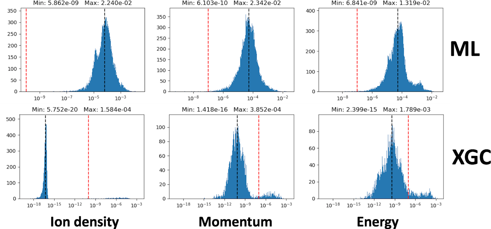
In order to declare success, it is necessary to look at how well the neural network can solve (4.1), i.e. how well it conserves particle density, momentum and energy. Looking at (4.8), we require each of the terms in the sum to be a minimum. Work still must be done to reduce the quantities in figure 6 to the threshold levels in XGC in case there is a drift-type machine learning error propagation in time, but even these results show promise for reaching the precision required for the XGC code. The benefit of course to using the machine learning algorithm is that the time to solution should be much faster compared to the Picard iteration solver. Further work into optimization schemes has demonstrated even more promising results. In particular, an augmented Lagrangian scheme, which will be detailed in a subsequent report, has extended this initial machine learning application down to an accuracy of $10^{-6}$.

Figure 6.

Comparison of conservation properties from XGC and from test set of neural network using machine learning (ML). The black vertical dashed lines represent the median value for the specific quantity. The red ones represent the target value (see (4.7)). Note that the $x$ axes (and $y$ axes) are different in both sets of plots.