II. POWER LAW CREEP MODEL

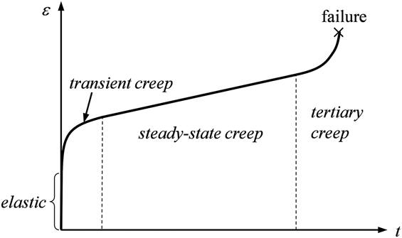
Creep describes the time-dependent response to an applied stress or strain; in this study, creep refers to viscoplastic material behavior. Three stages of creep can be observed in a creep test (Fig. 1). During transient or primary creep the strain rate decreases quickly and approaches a constant value. Has this constant value been reached steady-state or secondary creep has commenced. After a relatively long time, the strain rate begins to increase during tertiary creep until failure.

FIG. 1.

Stages of creep in uniaxial creep test.

The indentation creep test differs from the uniaxial creep insofar as the material is subject to a complex tri-axial stress state, which varies with position and time. Nonetheless, stress–strain rate relations for the two test types are usually formulated in an equal manner to allow direct comparison

(1)$$\eqalign{ & \dot \varepsilon = A\,{\sigma ^m}\;\;\;\;\;\;{\rm{uniaxial\ test}} \cr & \dot \varepsilon = B\,{\sigma ^m}\;\;\;{\rm{indentation\ test\ }}\left( {\sigma = P/{A_{\rm{p}}}} \right)\quad , \cr}$$

where m is the creep exponent, and A and B are creep coefficients ($\dot \varepsilon$ is further temperature-dependent, but this is not discussed here). The value of the creep stress exponent gives some information on the prevailing mechanism; a low m (≤1) indicates diffusion-controlled creep, m ≈ 2 grain boundary sliding-controlled creep and higher m dislocation climb-controlled creep. As the stress beneath the indenter varies with position, an equivalent stress is used, which may be defined as the ratio of indentation load P to projected area A _p (cross-sectional area of the indenter at current depth). Similarly, an equivalent strain rate can be defined as $\dot h/h$, $\dot h/\sqrt A$ or $\dot h/a$ where h, $\dot h = {{{\rm{d}}h} \mathord{\left/ {\vphantom {{{\rm{d}}h} {{\rm{d}}t}}} \right. \kern-\nulldelimiterspace} {{\rm{d}}t}}$ and a are indentation depth, indentation depth rate and impression radius, respectively. However, application of Eq. (1) requires that all deformation be only due to steady-state creep.

Taking in mind that the indentation test is usually a short-time test, transient creep is expected to affect the material behavior. Transient creep can be accounted for by applying the following equivalent stress–strain rate (σ–$\dot \varepsilon$) law^{Reference Ogbonna, Fleck and Cocks27}

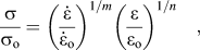(2)$${{\rm{\sigma }} \over {{{\rm{\sigma }}_{\rm{o}}}}} = {\left( \dot \varepsilon \over \dot \varepsilon_{\rm{o}}}}}} \right)^{{1 \mathord{\left/ {\vphantom {1 m}} \right. \kern-\nulldelimiterspace} m}}}{\left( {{{\rm{\varepsilon }} \over {{{\rm{\varepsilon }}_{\rm{o}}}}}} \right)^{{1 \mathord{\left/ {\vphantom {1 n}} \right. \kern-\nulldelimiterspace} n}}}\quad ,$$

where σ_o, ε_o, and $\dot \varepsilon_{\rm{o}}$ are reference stress, reference strain, and reference strain rate, respectively. For n → ∞, the response reduces to that of a material showing no hardening. For m = 1 and n → ∞, the material approaches a linear (Newtonian) viscous creeping material while the limit n → ∞ represents a steady-state creeping solid. The power law creep relation can be expressed in a time-hardening form

(3)$$\dot \varepsilon = C{\sigma ^k}{t^l}\quad ,$$

or a strain-hardening form

(4)$$\dot \varepsilon = {\left\{ {C\sigma _{}^k{{\left[ {\left( {l + 1} \right)\varepsilon } \right]}^l}} \right\}^{{1 \over {l + 1}}}}\quad ,$$

where ε is the cumulative strain, and C, k, and l are (temperature-dependent) creep constants. Physical considerations require that C and k be positive, and −1 < l ≤ 0. After differentiation with respect to time, the time-hardening power law creep relation can be written as^{Reference Ogbonna, Fleck and Cocks27}

(5)$$\dot \varepsilon = {\dot \varepsilon _{\rm{o}}}{\left( {{\sigma \over {{\sigma _{\rm{o}}}}}} \right)^{{{\rm{1}} \over {M{\rm{ + }}N}}}}{\left( {{t \over {{t_{\rm{o}}}}}} \right)^{ - {N \over {M{\rm{ + }}N}}}};\quad {\dot \varepsilon _{\rm{o}}} = \left( {{{{\varepsilon _{\rm{o}}}} \over {{t_{\rm{o}}}}}} \right)\left( {{N \over {M + N}}} \right)\quad ,$$

where ε_o is the strain after time t _o at reference stress σ_o; M (>0) and N (<1) are the reciprocals of m and n in Eq. (2), respectively. Combining Eqs. (3) and (5) yields the following three relations

(6)$$C = {\dot \varepsilon _{\rm{o}}}\sigma _{\rm{o}}^{ - {{\rm{1}} \over {M{\rm{ + }}N}}}\,t_{\rm{o}}^{{N \over {M{\rm{ + }}N}}};\quad k = {1 \over {M + N}};\quad l = - {N \over {M + N}}\quad .$$

To obtain creep coefficient C from the strain-hardening creep relation, we insert Eq. (6) into Eq. (4)

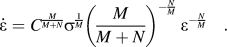(7)$$\dot \varepsilon = {C^{{M \over {M + N}}}}{\sigma ^{{1 \over M}}}{\left( {{M \over {M + N}}} \right)^{ - {N \over M}}}\;{\varepsilon ^{ - {N \over M}}}\quad .$$

As the final goal is to find C and m, we rewrite Eq. (7) in a form that allows direct extraction of these creep parameters

(8)$$\dot \varepsilon = K{\left( {\sigma \;{\varepsilon ^{ - {1 \mathord{\left/ {\vphantom {1 n}} \right. \kern-\nulldelimiterspace} n}}}} \right)^m}\quad ,$$

where

(9)$$K = {C^{{{m + n} \over n}}}{\left( {{{m + n} \over n}} \right)^{{m \over n}}}\quad .$$

In this study, n is assumed to be known. m and K in Eq. (8) can be readily found by plotting $\log \left( {\sigma \,{\varepsilon ^{{{ - 1} \mathord{\left{\vphantom {{ - 1} n}} \right\kern-\nulldelimiterspace} n}}}} \right) - \log \dot \varepsilon$ data and determining the curve's slope (=m) and intercept with the ordinate (=K). C is then calculated by Eq. (9).

III. FE ANALYSIS OF CREEP INDENTATION TEST CONSIDERING TRANSIENT CREEP

Instead of defining global equivalent strain and stress measures, which can hardly represent the complex deformation field beneath the indenter, we use the equivalent Mises strain and stress at a fixed position inside the material (observation point), where the material response is hardly affected by elastic properties so that creep parameters can be obtained accurately. Since subsurface stress–strain data cannot be obtained from real indentation tests and since the approach should be applicable to a large range of materials, we apply FEM as the tool for investigation.

A. FE model

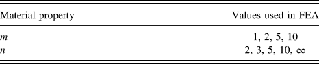
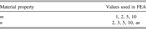
To simulate spherical indentation of a power law-creeping material, a 2D axisymmetric FE model consisting of 4-node axial symmetry elements [CAX4 (Ref. 32)] is used (Fig. 2). Our previous work revealed that the use of eight-node CAX8 elements in Abaqus leads to a discontinuous equivalent plastic strain at the mid-nodes.^{Reference Lee, Lee and Pharr33} The lower degree of the CAX4 shape function is compensated for by using a finer mesh. The inner region, where large deformations and deformation gradients are expected, is highly refined, while the mesh coarsens with distance from the indenter. The mesh around the potential observation point (see Sec. III. B) is densified. Regions of different mesh densities are interconnected by imposing multi-point constraints. This is acceptable because large deformations are confined to the very vicinity of the contact region. The model consists of approximately 16,000 elements. The indenter is modeled as a rigid body, and the contact between indenter and specimen is assumed frictionless. The bottom of the specimen is constrained in z-direction, whereas the right boundary remains unconstrained. The size of the model is chosen so large that influences from the boundaries are negligible. Since it is found to provide better convergence than the CLH test, for the indentation creep test the load is applied with a constant rate of depth as in the CRD test. Table I lists the values of m and n used in the FE analyses (FEAs).

FIG. 2.

FE mesh for creep indentation analysis.

TABLE I.

Values of material properties m and n used in FEA.

B. Equivalent strain rate and observation point

For the evaluation of creep coefficient C and creep exponent m of a material, a point in the FE model is to be determined where throughout loading the strain rate remains on a relatively small level and has low gradients and where the elastic strain is negligible compared with the total Mises strain. The material response at this point is then compared with the response in the uniaxial creep test. Note that the use of an observation point is only practical in FE simulations and cannot be applied to the real indentation test. However, the observation point serves to establish the functions that relate load–depth data from the indentation test to the creep properties C and m.

The total Mises (or equivalent) strain ε_tot can be decomposed into equivalent elastic strain ε_e and equivalent creep strain ε_c

(10)$${\varepsilon _{{\rm{tot}}}} = \sqrt {{2 \over 3}\varepsilon _{ij}^{{\rm{dev}}}\varepsilon _{ij}^{{\rm{dev}}}\,} = {\varepsilon _{\rm{e}}} + {\varepsilon _{\rm{c}}}\quad ,$$

where $\varepsilon _{ij}^{{\rm{dev}}}$ denote the deviatoric strain components. Indentation is performed to h _t/D = 0.1; the total time of load application is t _c = 100 s. We assume a material with m = 5, n = 10, C = 8.73 × 10⁻² MPa^−10/3 s^−2/3, E = 1000 GPa, ν = 0.3, and ε_o = 0.001. The ratio of Young's modulus to yield strength is chosen high so to minimize the effect of ε_e. ε_tot, ε_e and ε_c are obtained at different relative depths l/D along the z-axis (r = 0), where l denotes the vertical distance from the initial material surface and D is the indenter diameter. Figure 3 shows for l/D = 0, 0.1, and 0.2, the change of ε_tot, ε_e and ε_c and their time derivatives ${\dot \varepsilon _{{\rm{tot}}}},{\dot \varepsilon _{\rm{e}}} {\rm{and}} {\dot \varepsilon _{\rm{c}}}$—the derivatives are calculated by dividing each strain increment by the corresponding time increment—with time t. Along the z-axis, the elastic strain is negligible compared with the creep strain, so that we can write ${\varepsilon _{\rm{c}}}\dot = {\varepsilon _{{\rm{tot}}}}$ (the sign $\dot =$ denotes here “approaches the limit”). Similarly, the elastic strain rate is nearly zero, and hence ${\dot \varepsilon _{\rm{c}}}\dot = {\dot \varepsilon _{{\rm{tot}}}}$. The initial strain rate and the final (and more or less constant) strain rate are large at the surface (l/D = 0). Inside the material, the strain rate increases from zero and reaches a peak before it approaches an approximately constant value from above. With increasing l/D, the strain rate peaks and the final values decrease. To avoid too small strain rates for higher l/D, we choose as the point of observation r = 0, l/D = 0.2, a point where the elastic strain amounts to less than 1% of the total strain. Because stress and strain rate at this point are only insignificantly affected by elastic material properties but sensitive to creep properties, creep properties can be obtained accurately from the indentation load–displacement curve.

FIG. 3.

ε_tot, ε_e, ε_c–t curves (a) and $\dot \varepsilon$_tot, $\dot \varepsilon$_e, $\dot \varepsilon$_c–t curves (b) for diverse l/D.

C. Comparison with uniaxial tensile creep test

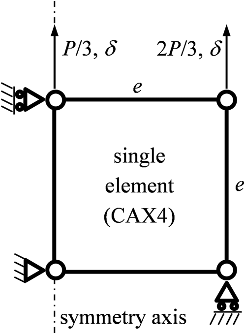
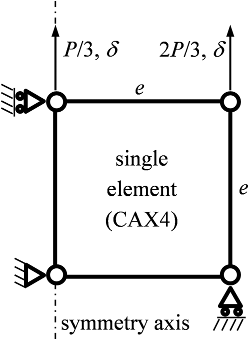
To validate that the observation point is appropriate for extracting uniaxial creep parameters, we perform CRD type and CLH type uniaxial tensile creep tests using an FE model consisting of a single 4-node axisymmetric element (CAX4) of edge length e (Fig. 4), and compare the material response with the one from indentation creep test. The left nodes are constrained in horizontal direction, and the bottom nodes in vertical direction. For CRD creep tensile tests, the top nodes are displaced vertically by δ/e = 1/600 ≈ 0.0167. For CLH creep tensile tests, a load P is imposed on the top surface, so that an equally high tensile displacement δ/e is obtained. As for the indentation test, test duration is set to t _c = 100 s.

FIG. 4.

Single element analysis model.

Using the same material as above, ε_tot, ε_e, ε_c and the corresponding rates are plotted against time t (Fig. 5). In the CLH test, deformation is dominated by creep strains throughout the test so that ${\dot \varepsilon _{\rm{c}}}\dot = {\dot \varepsilon _{{\rm{tot}}}}$, whereas in the CRD test, the strain is in the beginning mainly elastic but becomes increasingly creep-dominated (${\dot \varepsilon _{\rm{e}}} \to 0$). Figure 6 depicts corresponding strain rate-equivalent stress curves. In the CLH test, in accordance with transient creep, the initially high creep strain rate decreases sharply and then seems to approach a constant value. The stress hardly decreases from its initial value of P/(πe ²) ≈ 106.1 MPa. On the contrary, in the CRD test the stress increases relatively slowly with $\dot \varepsilon$ from zero to its final value. In neither test the strain rate has assumed a constant value after t _c = 100 s, which shows that pure steady-state creep has not yet been established.

FIG. 5.

ε_tot, ε_e, ε_c–t curves (a) and $\dot \varepsilon$_tot, $\dot \varepsilon$_e, $\dot \varepsilon$_c–t curves (b) from single element analyses of CRD and CLH type uniaxial tensile tests.

FIG. 6.

Logarithmic $\dot \varepsilon$ −σ curves from single element simulations of CLH (a) and CRD tests (b).

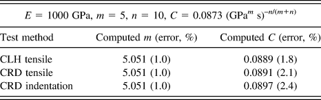
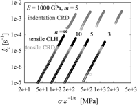
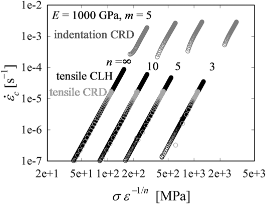
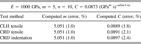
For the materials with m = 5 and diverse n, results from the CLH and the CRD tensile tests are compared with data from the CRD creep indentation analysis, obtained at the point of observation (Fig. 7). Excluding indentation creep test data obtained at very low depths (which are numerically critical), data points from all tests for a certain n value lie on the same straight line. Fitting data to Eq. (8) by the least-squares method, resulting values for m and C are very close to the FEA input values, with a maximum deviation of 1.0 and 2.4%, respectively (Table II). m and C can thus be determined accurately from the indentation analysis stress and strain (rate) data obtained at the observation point. In Sec. IV, we will investigate the influence of material properties m and n on the material response to indentation.

FIG. 7.

Logarithmic $\dot \varepsilon$_c–(σε^−1/n) curves from CRD and CLH tensile tests and CRD indentation test for m = 5 and diverse n.

TABLE II.

Comparison of creep properties from simulated CRD, CLH tensile tests, and CRD indentation test with FE input values.

IV. EVALUATION OF CREEP PROPERTIES

Relying on FEA the material response is investigated at the point of observation by varying the creep parameters as listed in Table I. Two dimensionless variables ξ and ψ are introduced to characterize the material response. The former represents the equivalent strain rate and is defined as

(11)$$\xi \equiv \dot \varepsilon \;t\quad ,$$

where $\dot \varepsilon$ is the equivalent strain rate. The second dimensionless variable, ψ, represents the equivalent stress and is defined by the indentation load P normalized by the nominal force σD ²

(12)$$\psi \equiv {P \over {\sigma {D^2}}}\quad .$$

Note that by contrast with $\dot \varepsilon$ and σ, both ξ and ψ are insensitive to t _c and E. To study the influences of m and n on ξ at the observation point, ξ is plotted against the normalized indentation depth h/D for diverse hardening exponents n and m = const. as well as for diverse creep exponents m and n = const. As in Fig. 8 for the examples m = 1, 10 (variation of n) and n = 3, ∞ (variation of m), ξ increases monotonically with increasing h/D for all combinations of n and m. To convert h/D data to ξ data, we propose the following mapping function

(13)$$\eqalign{ &#x0026; \xi = f_i^\xi \left( {m,n} \right){\left( {{h \over D}} \right)^i} \cr &#x0026; f_i^\xi \left( {m,n} \right) = \alpha _{ij}^\xi \left( m \right)\;{n^{ - j}};\quad \alpha _{ij}^\xi \left( m \right) = \beta _{ijk}^\xi \;{m^{ - k}} \cr &#x0026; i{\rm{\ }} = {\rm{1,}} \ldots ,{\rm{3}};j = {\rm{\ }}0, \ldots ,{\rm{3}};k = 0, \ldots ,{\rm{3}}\quad {\rm{,}} \cr}$$

where summation over indices is implied. The fitting coefficients $\beta _{ijk}^\xi$ are given in Table III. The regression curves, depicted in Fig. 8 as red solid lines, agree well with the FE data. The strain data is obtained by numerically integrating (trapezoidal method) the strain rate over t from zero to the time when $\dot \varepsilon$ is attained

(14)$$\varepsilon = \int_0^t {\dot \varepsilon \,{\rm{d}}t\quad .}$$

FIG. 8.

ξ–h/D data for diverse n and m = 1, 10 (a and b) and for diverse m and n = 3, ∞ (c and d); red lines depict the corresponding regression curves.

TABLE III.

Coefficients $\beta _{ijk}^\xi$ of Eq. (13).

In Fig. 9 we can see how hardening and creep exponents influence the relation between ψ and h/D for m = 1, 10 (variation of n) and for n = 3, ∞ (variation of m). As ξ above, ψ increases with depth and the difference between initial and final ψ values becomes larger for higher m and n. ψ is expressed by

(15)$$\eqalign{ &#x0026; \psi = f_i^\psi \left( {m,n} \right){\left( {{h \over D}} \right)^i} \cr &#x0026; f_i^\psi \left( {m,n} \right) = \alpha _{ij}^\psi \left( m \right)\;{n^{ - j}};\quad \alpha _{ij}^\psi \left( m \right) = \beta _{ijk}^\psi \;{m^k} \cr &#x0026; i{\rm{\ }} = 0, \ldots ,{\rm{2}};j = {\rm{\ }}0, \ldots ,{\rm{3;\ }}k = 0, \ldots ,{\rm{3}}\quad {\rm{,}} \cr}$$

where, again, summation over indices is implied. The coefficients $\beta _{ijk}^\psi$ are listed in Table IV. Red solid lines in Fig. 9 depict the regression curves.

FIG. 9.

Regressed ψ–h/D curves for m = 2 (a and c) and n = 5 (b and d).

TABLE IV.

Coefficients $\beta _{ijk}^\xi$ of Eq. (15).

Since, as noted before, the material response at the observation point is only insignificantly affected by elastic properties and since further β^ξ and β^ψ matrices are derived from parameter studies where m and n are varied over a large range, both matrices can be considered material-independent. Now that the β matrices have been evaluated, indentation load–depth data can be converted to equivalent stress and strain (rate) data at the observation point, which then allow extraction of creep coefficient and exponent.

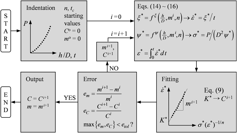
Figure 10 outlines the iterative procedure for the evaluation of creep properties C and m from short-time spherical indentation tests. Indentation load–depth history data, n and t _c enter as input values; starting values for m and C are m ^o = C ^o = 0. First the load–depth history data are converted to stress–strain–strain rate data at the point of observation. To do so, we calculate (temporary) ξ* and ψ* data by means of Eqs. (13) and (15) using the coefficients in Tables III and IV, respectively. These data are then converted to ${\dot \varepsilon ^ * }$, σ*, and ε* is calculated by Eq. (14). Second, from the $\dot \varepsilon - \left( {\sigma {\varepsilon ^{{{ - 1} \mathord{\left{\vphantom {{ - 1} n}} \right\kern-\nulldelimiterspace} n}}}} \right)$ plot, new values for m and C [via K*, Eq. (9)], m ⁱ⁺¹ and C ⁱ⁺¹, are calculated and compared with the values assumed at the beginning of the loop. If the convergence criterion is not met, i.e., if the relative changes of both m ⁱ⁺¹ and C ⁱ⁺¹ with respect to m ⁱ and C ⁱ exceed a specified tolerance (in our case e _tol = 10⁻⁷), m ⁱ⁺¹ and C ⁱ⁺¹ are returned to the start of the loop. The procedure is repeated until the convergence criterion is satisfied; the last m ⁱ⁺¹ and C ⁱ⁺¹ are the sought-for creep parameters of the material.

FIG. 10.

Flow chart for determining C and m (superscript * denotes temporary value).

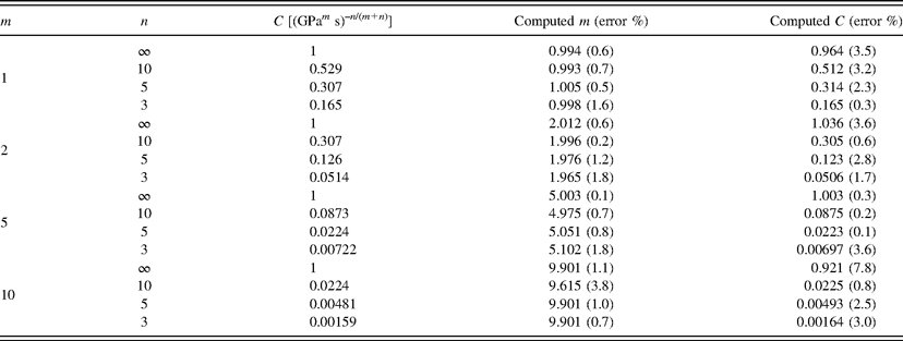
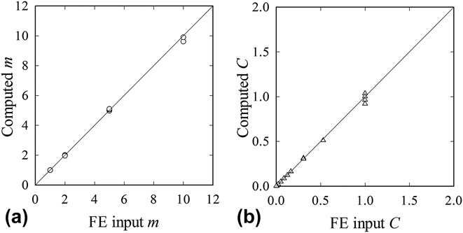
Figure 11 shows the strain rate–stress data computed by the algorithm in Fig. 10 using load–displacement data from indentation; the red curves represent the FE input data. Note that the FE input data are the data that are to be found in actual indentation experiments. Creep exponent m and creep coefficient C are listed in Table V. The properties obtained from the load–depth curve deviate in average less than 1.1% for m and less than 2.3% for C from the FE input values (Fig. 12).

FIG. 11.

Comparison of strain rate–stress data obtained by the algorithm in Fig. 10 with Eq. (8) for all combinations of m and n.

TABLE V.

Comparison of creep properties determined by the algorithm in Fig. 10 with FE input values (=properties to be found) for all combinations of m and n.

FIG. 12.

Comparison of (a) computer m and (b) computer C with FE input values (=properties to be found).

V. CONCLUDING REMARKS

This work provides an efficient way of deriving uniaxial creep parameters from spherical indentation load–depth data and the material’s hardening exponent n. Transient effects are considered through the strain hardening creep law of Ogbonna et al.^{Reference Ogbonna, Fleck and Cocks27} Instead of global equivalent measures, (Mises) equivalent stress and strain are obtained locally at a subsurface observation point where the strain rate–stress behavior is hardly affected by elastic material properties and is in a good agreement with that observed in uniaxial tensile tests which were simulated in parallel. Introducing dimensionless indentation variables (evaluated at the observation point), we then established, based on FE results for a large range of m and n, functions that map the indentation load–depth data (together with indenter diameter, hardening exponent, and creep time) to stress–strain (rate) data. The $\dot \varepsilon - \left( {\sigma {\varepsilon ^{{{ - 1} \mathord{\left{\vphantom {{ - 1} n}} \right\kern-\nulldelimiterspace} n}}}} \right)$ plot then allows determination of C and m in an iterative manner. Finally an algorithm is presented that illustrates the extraction of creep coefficient and exponent from load–depth data. Results acquired by the proposed method agree very well with the sought-for FE input data.