1. Introduction
We study nonlinear (NL) three-dimensional (3D) effects, characterized by spanwise wavelength, on the flapping dynamics of a flag in a uniform fluid flow, allowing for spanwise variations of structural displacement and fluid flow. In this initial study, we consider periodic spanwise variations, ignoring spanwise edge effects. This investigation is fundamental to understanding the full dynamics of a 3D flapping flag. It is also relevant to a wide range of applications involving thin membranes such as the biomechanics of snoring (e.g. Auregan Reference Auregan1995; Huang Reference Huang1995); the performance of printing presses (e.g. Watanabe et al. Reference Watanabe, Suzuki, Sugihara and Sueoka2002); the flow–structure interactions of myriad organisms and their size scale adaptations in aquatic ecosystems (e.g. Nikora Reference Nikora2010); the waving motions induced in flexible blades due to canopy-sized vortices (e.g. Nepf Reference Nepf2012); and novel designs for flow energy harvesters (e.g. Taylor et al. Reference Taylor, Burns, Kammann, Powers and Welsh2001; Michelin & Doaré Reference Michelin and Doaré2013).
The mechanisms and patterns of behaviour of the flag flapping problem continue to generate significant scientific interest as a fundamental problem of fluid–structure interaction. The study of the strictly two-dimensional (2D) flag flapping problem has been the focus of a number of experimental, analytical, and numerical studies. Many of these are motivated by the 2D experiment of Zhang et al. (Reference Zhang, Childress, Libchaber and Shelley2000) where the response of flexible filaments was examined in a flowing soap film. They found two distinct states for a single filament: the stretched-straight state and the self-sustained flapping state. Conducting experiments in water, Shelley, Vandenberghe & Zhang (Reference Shelley, Vandenberghe and Zhang2005) reported that it is much harder to realize flapping, and special treatment was required to bring the membrane mass up to a sufficient value to realize flapping. They found similar results to those of the air experiments for stability, response, and bistability with changing flow velocity, and that the Strouhal frequency is consistent with that of animal locomotion. Connell & Yue (Reference Connell and Yue2007) (hereafter CY) performed an analysis of the flag flapping stability and response for the 2D problem through a combined analytical and numerical investigation. They identify the important parameters in relation to their influence on the system response: the structure-to-fluid mass ratio
 ${\it\mu}={\it\rho}_{s}h/({\it\rho}_{f}L)$
, and the Reynolds number
 $\mathit{Re}_{L}=VL/{\it\nu}$
for a two-dimensional body of length
 $L$
, mass-per-length
 ${\it\rho}_{s}h$
, and bending rigidity
 $EI$
, in a fluid flow of density
 ${\it\rho}_{f}$
, viscosity
 ${\it\nu}$
, and flow speed
 $V$
, both stabilizing for lower values. Using direct numerical simulations, CY found three main regimes of the response: fixed-point stability, limit-cycle oscillation, and chaotic flapping. Shelley & Zhang (Reference Shelley and Zhang2011) presents a review of the recent advances in experiments and theoretical understanding of the 2D flag flapping problem.
There are relatively fewer studies of the 3D aspects of the flag flapping problem. Eloy, Souilliez & Schouveiler (Reference Eloy, Souilliez and Schouveiler2007) considered the stability of a plate with finite span (including edge effects) assuming inviscid flow, obtaining different modes of flutter, and confirmed it by an experimental study in Eloy et al. (Reference Eloy, Lagrange, Souilliez and Schouveiler2008). Kim & Peskin (Reference Kim and Peskin2007) simulated the 3D flag problem using the penalty immersed boundary method, and qualitative observations were made of the mode shapes including the effects of gravity. Using similar computations, Huang & Sung (Reference Huang and Sung2010) studied the nonlinear dynamics of the coupled fluid–flag system after set-in of flapping. They found a significant 3D effect on the vortical structures for smaller span, and its stabilizing influence through a reduction of the pressure difference across the flag. Doare, Mano & Ludena (Reference Doare, Mano and Ludena2011) show that a 2D model always underestimates the critical velocity relative to 3D experimental data. By bounding the flexible plate between two spanwise walls, they are able to quantify the difference due to 3D spanwise effects. For relatively large aspect ratios where span edge effects might be neglected, an analysis assuming periodic boundary condition and discrete spanwise wavelengths can be considered. Argentina & Mahadevan (Reference Argentina and Mahadevan2005) discussed the stabilizing influence of finite 3D wavelengths using a 2D flag model with data from 3D simulation, and show that the instability threshold is higher in the presence of spanwise modes.
The present flag problem possesses a number of distinct features as compared to a cylinder. The 3D deformation of the flag surface (with a non-moving leading edge) is an integral part of the fluid–structure interaction; vortex shedding from a (moving) trailing edge differs qualitatively from the unsteady separation from two sides of a bluff cylinder; and there is no equivalent ‘diameter’ parameter other than the (a priori unknown) trailing-edge amplitude. Furthermore, the (material) mass of the flag is typically much smaller than the added mass, although the former (relative to fluid mass) still plays a critical role. The differences between the behaviour of flag flapping and vortex shedding from cylinders is discussed in a brief communication by Huber (Reference Huber2000).
In the present study, we investigate the effect of 3D spanwise motions on the dynamics of flag flapping. Specifically we consider (periodic) spanwise variations characterized by
 ${\it\gamma}\equiv S/L$
, where
 $S$
is the fundamental spanwise wavelength and
 $L$
is the chord length. We first perform a linear stability analysis of the flag motion, obtaining a stability condition in terms of spanwise and chordwise wavenumbers of the (un)stable mode, and the physical fluid–structural parameters
 ${\it\mu}$
and
 $\mathit{Re}_{L}$
of the problem. To validate the linear analysis and obtain longer time NL evolution, we develop a direct numerical simulation (FSDS3D) for this problem. FSDS3D solves for the 3D fully coupled dynamics of a flag in an incompressible flow with arbitrarily large flag displacements, employing a boundary-fitted moving grid which resolves the boundary layer on the body. A systematic set of FSDS3D simulations are obtained for a range of values of
 ${\it\gamma}$
and
 ${\it\mu}$
, with a chord-based Reynolds number
 $\mathit{Re}_{L}=1000$
. We derive, for use as initial conditions, 3D normal (standing) modes for the flag. We further consider the evolution with and without the presence of a (spanwise) cross-flow.
We investigate a number of unanswered questions regarding the effects of 3D spanwise motions characterized by dimensionless spanwise wavelength
 ${\it\gamma}$
on flag flapping dynamics. How does finite
 ${\it\gamma}$
affect the stability and response of a flag, and what are the underlying cause and mechanism? How does the NL (multi-mode) evolution differ in the absence or presence of cross-flow for different
 ${\it\gamma}$
? What are the characteristics of 3D flapping and wake vortex responses? What governs the lift and drag on the flag under 3D motion? These are some of the key questions we address here.
The paper is organized as follows. Section 2 defines the problem we consider and the relevant system parameters. A description of the FSDS3D direct numerical simulation method is given in § 3, and select validation results are given in appendix A. The linear stability analysis is given in § 4. A systematic set of FSDS3D results validating the linear stability predictions, and elucidating the coupled structural and vortex behaviour of the system, are presented in § 5. Concluding remarks are in § 6.
2. Problem statement
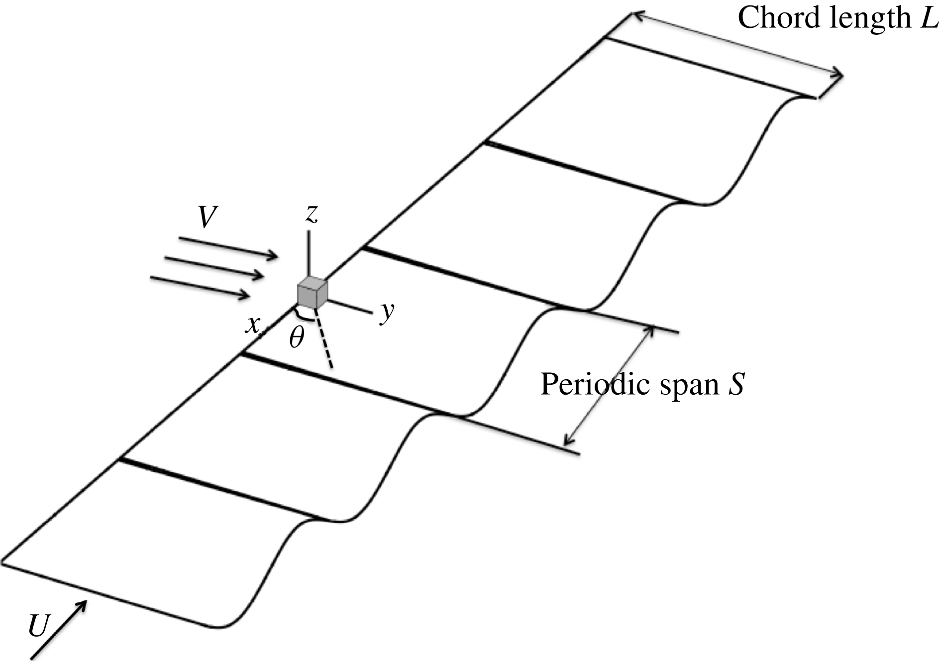
We model a 3D flag as a thin membrane with negligible bending rigidity, pinned at the leading edge (LE) and free at the trailing edge (TE), placed in a uniform incompressible viscous inflow, in the absence of gravity, as shown in figure 1, where
 $x$
,
 $y$
and
 $z$
are respectively the cross-flow span, streamwise chord and flag normal directions. We consider spanwise periodicity of length
 $S$
for the structural motion and fluid flow, and focus on the effect of three-dimensionality measured by the parameter
 ${\it\gamma}\equiv S/L$
, where
 $L$
is the (unstretched) streamwise chord length.
Problem definition: the flapping motion of a 3D flag, with chord length
 $L$
, uniform incoming flow
 $V$
, with spanwise cross-flow component
 $U$
and cross-flow angle
 ${\it\theta}$
and structural motions of fundamental periodic length
 $S$
.

The geometrically nonlinear equation of motion for the 3D flag is
 $$\begin{eqnarray}{\it\rho}_{s}h\frac{\partial ^{2}\boldsymbol{x}}{\partial t^{2}}-\frac{\partial }{\partial s_{1}}\left(T_{1}\frac{\partial \boldsymbol{x}}{\partial s_{1}}\right)-\frac{\partial }{\partial s_{2}}\left(T_{2}\frac{\partial \boldsymbol{x}}{\partial s_{2}}\right)-\frac{\partial }{\partial s_{1}}\left(M\frac{\partial \boldsymbol{x}}{\partial s_{2}}\right)-\frac{\partial }{\partial s_{2}}\left(M\frac{\partial \boldsymbol{x}}{\partial s_{1}}\right)=\boldsymbol{F}_{f},\end{eqnarray}$$
where
 $s_{1}$
,
 $s_{2}$
are the Lagrangian coordinates along the chordwise and spanwise directions respectively, and
 $\boldsymbol{x}$
is the position vector on the flag. Structural parameters are
 ${\it\rho}_{s}$
for the structural density,
 $h$
for the body thickness and
 ${\it\nu}_{s}$
for the Poisson ratio.
 $T_{1}$
,
 $T_{2}$
are the internal tension forces in the
 $s_{1}$
,
 $s_{2}$
directions respectively and
 $M$
is the moment due to shear stresses in the plane of the flag. Note that in (2.1) the bending rigidity is not taken into account. In a spanwise-periodic context, finite extensibility must be included in order for there to be spanwise structural displacements. We therefore include a (small) extensibility, characterized by the spanwise strain due to the variation of
 $T_{2}$
along
 $s_{2}$
.
The fluid-dynamic governing equations and associated forcing to the flag are similar to CY for the 2D problem. Fluid forcing to the body is through the fluid-dynamic stresses given by
 $$\begin{eqnarray}\displaystyle \boldsymbol{F}_{f}={\it\tau}_{ij}\hat{n}_{j}, & & \displaystyle\end{eqnarray}$$
where
 $\hat{n}_{j}$
is the upward normal vector and elements of the stress tensor
 ${\it\tau}_{ij}$
are derived from the fluid dynamics at the surface as
 $$\begin{eqnarray}\displaystyle {\it\tau}_{ij}={\it\nu}{\it\rho}_{f}\left(\frac{\partial u_{i}}{\partial {\it\xi}_{j}}+\frac{\partial u_{j}}{\partial {\it\xi}_{i}}\right)-{\it\delta}_{ij}p. & & \displaystyle\end{eqnarray}$$
The fluid-dynamic solution comes from the Navier–Stokes equations, enforcing conservation of momentum and mass for incompressible flow:
 $$\begin{eqnarray}\displaystyle & \displaystyle \frac{\partial \boldsymbol{v}}{\partial t}+(\boldsymbol{v}\boldsymbol{\cdot }\boldsymbol{{\rm\nabla}})\boldsymbol{v}=-\frac{1}{{\it\rho}_{f}}\boldsymbol{{\rm\nabla}}p+{\it\nu}{\rm\nabla}^{2}\boldsymbol{v}, & \displaystyle\end{eqnarray}$$
 $$\begin{eqnarray}\displaystyle & \displaystyle \boldsymbol{{\rm\nabla}}\boldsymbol{\cdot }\boldsymbol{v}=0. & \displaystyle\end{eqnarray}$$
 $$\begin{eqnarray}\displaystyle \boldsymbol{v}=\partial \boldsymbol{x}/\partial t. & & \displaystyle\end{eqnarray}$$
We impose,
 $\boldsymbol{v}=(U,V)$
, the uniform inflow far upstream, where
 $U=(\neq )0$
in the absence (presence) of cross-flow. These governing equations, coupled by the external forcing to the structure and the kinematic boundary condition of the flow field, describe the complete coupled fluid–flag problem including effects of added mass, viscous drag, and vortex shedding into the wake.
3. The coupled direct numerical simulation model: FSDS3D
For this study, we extend the coupled fluid–structure direct simulation model (FSDS) developed in CY to the 3D problem (FSDS3D) allowing for periodic spanwise motions. The fluid-dynamic solver is a 3D direct numerical simulation of the incompressible Navier–Stokes equation, solved on a grid moving with the structural inner boundary. The 3D structural-dynamic direct simulation (SDS) represents a thin membrane which is geometrically nonlinear, allowing arbitrarily large displacements. The 3D fluid-dynamic solver (FDS) framework is developed in CY; however, a brief discussion of the numerical solver is given to highlight the inclusion of the spanwise dimension in the solution.
3.1. The fluid-dynamic solver (FDS)
The fluid-dynamic direct simulation solver (FDS) is as described in CY, with the inclusion now of a spanwise dimension with periodic boundary conditions. The computational (
 ${\it\xi},{\it\rho},{\it\theta}$
) and physical (
 $x,y,z$
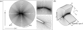
) coordinate directions are depicted in figure 2. The coordinate dependences between these are
 $$\begin{eqnarray}\left.\begin{array}{@{}cc@{}}x({\it\xi}) & {\it\xi}(x)\\ y({\it\xi},{\it\rho},{\it\theta},{\it\tau}) & {\it\rho}(x,y,z,t)\\ z({\it\xi},{\it\rho},{\it\theta},{\it\tau}) & {\it\theta}(x,y,z,t)\\ t({\it\tau}) & {\it\tau}(t),\end{array}\right\}\end{eqnarray}$$
where time is represented in the physical domain by
 $t$
and in the computational domain by
 ${\it\tau}$
. The mappings do not require the inner boundary to be straight or stationary, but the
 ${\it\rho}{-}{\it\theta}$
planes must be parallel and evenly spaced. As the inner boundary moves during a simulation, a two-dimensional elliptical grid solver is used in the
 ${\it\rho}{-}{\it\theta}$
planes, and the associated grid velocities are calculated numerically.
(a) Cross-section of grid. Arrows represent an inflow condition at the outer boundary. (b) Computational grid for the FDS solution shown with cut-out for clarity. The computational (
 ${\it\xi},{\it\rho},{\it\theta}$
) and physical (
 $x,y,z$
) coordinate directions are also indicated. Periodic boundary conditions are applied on the
 $x=0$
,
 $S$
surfaces.

A two-dimensional cross-section shown in figure 2(a) shows a slice of the physical domain with the corresponding computational grid. The increasing resolution of the grid toward the inner boundary of the body represents the importance of accurately solving the flow at the body boundary. The problem of the need for a complicated curvilinear coordinate system is approached by defining a computational domain where the directions are aligned exactly with the grid. The grid lines radiating from the inner body to the outer body are designated the direction
 ${\it\rho}$
, the lines circumscribing the inner cylinder are designated the direction
 ${\it\theta}$
, and the axial direction is designated
 ${\it\xi}$
.
The mapped derivatives are used in solution to the Navier–Stokes equation, non-dimensionalized by the chord length
 $L$
, the incoming flow speed
 $V$
, and the fluid density
 ${\it\rho}_{f}$
. The time integration method used is the second-order backwards difference scheme as discussed in Strikwerda (Reference Strikwerda1997) and Li & Tang (Reference Li and Tang2001). This implicit method offers stability with second-order accuracy, and gives the semi-discrete form
 $$\begin{eqnarray}\displaystyle \frac{3\boldsymbol{v}^{n+1}-4\boldsymbol{v}^{n}+\boldsymbol{v}^{n-1}}{2{\rm\Delta}t}+((\boldsymbol{v}^{n+1}-\boldsymbol{v}_{g}^{n+1})\boldsymbol{\cdot }\boldsymbol{{\rm\nabla}})\boldsymbol{v}^{n+1}=-\boldsymbol{{\rm\nabla}}p^{n+1}+\frac{1}{\mathit{Re}_{L}}{\rm\nabla}^{2}\boldsymbol{v}^{n+1}, & & \displaystyle\end{eqnarray}$$
where
 $\boldsymbol{v}_{g}$
is the velocity of the moving grid. All spatial derivatives are taken as second-order centred differences, excepting those in the convective term which use the third-order upwinding scheme of Kawamura & Kuwahara (Reference Kawamura and Kuwahara1984) (see also Li Reference Li1997). The pressure is found with a Poisson equation obtained with the projection method of Chorin (Reference Chorin1968) (see also Armfield Reference Armfield1991). The solution method and validation study for the FDS model are described in CY, with more details in Connell (Reference Connell2006).
3.2. The structural-dynamic solver (SDS)
We develop a robust nonlinear 3D structural solver capable of simulating a thin flexible membrane with arbitrary orientation and configuration. Following the approach in CY, we derive the equations in global Cartesian coordinates using Hamilton’s principal. The resulting model describes a nonlinear flexible membrane capable of large displacements. For thin membranes with thickness much smaller than transverse displacement, the stresses in the normal direction, and rotational inertia about the tangential directions can all be ignored. In the theoretical formulation (cf. (2.1)), bending stiffness in the flag is considered negligible. In the numerics, however, following e.g. Triantafyllou & Howell (Reference Triantafyllou and Howell1994), a small bending stiffness (
 $K_{B}=EI[{\it\rho}_{f}V^{2}L^{3}]^{-1}=O(10^{-4})$
) is added to smooth out the flag surface whenever positive tension vanishes at some point in the flag.
The equation of motion (including bending rigidity) for the thin, geometrically nonlinear flag is simplified (upon linearization about small thickness and small extensional strain):
 $$\begin{eqnarray}\underbrace{e1\frac{\partial ^{2}\boldsymbol{x}}{\partial t^{2}}}_{{\it\Phi}^{k}}+\underbrace{e2\frac{\partial ^{4}\boldsymbol{x}}{\partial {s_{1}}^{4}}}_{{\it\Phi}_{2D}^{b}}-\underbrace{e3\frac{\partial }{\partial s_{1}}\left(\left(1-\left(\frac{\partial \boldsymbol{x}}{\partial s_{1}}\boldsymbol{\cdot }\frac{\partial \boldsymbol{x}}{\partial s_{1}}\right)^{-1/2}\right)\frac{\partial \boldsymbol{x}}{\partial s_{1}}\right)}_{{\it\Phi}_{2D}^{s}}+\underbrace{{\it\Pi}}_{3D}=\boldsymbol{F},\end{eqnarray}$$
 $$\begin{eqnarray}\displaystyle \underbrace{{\it\Pi}}_{3D} & = & \displaystyle \underbrace{e2\left(2\frac{\partial ^{4}\boldsymbol{x}}{\partial {s_{1}}^{2}\partial {s_{2}}^{2}}+\frac{\partial ^{4}\boldsymbol{x}}{\partial {s_{2}}^{4}}\right)}_{{\it\Phi}_{3D}^{b}}\underbrace{-e3\frac{\partial }{\partial s_{1}}\left(\left[{\it\nu}_{s}\left(1-\left(\frac{\partial \boldsymbol{x}}{\partial s_{2}}\boldsymbol{\cdot }\frac{\partial \boldsymbol{x}}{\partial s_{2}}\right)^{-1/2}\right)\right]\frac{\partial \boldsymbol{x}}{\partial s_{1}}\right)}_{{\it\Phi}_{3D}^{s}}\nonumber\\ \displaystyle & & \displaystyle \underbrace{-\,e3\frac{\partial }{\partial s_{2}}\left(\left[\left(1-\left(\frac{\partial \boldsymbol{x}}{\partial s_{2}}\boldsymbol{\cdot }\frac{\partial \boldsymbol{x}}{\partial s_{2}}\right)^{-1/2}\right)+{\it\nu}_{s}\left(1-\left(\frac{\partial \boldsymbol{x}}{\partial s_{1}}\boldsymbol{\cdot }\frac{\partial \boldsymbol{x}}{\partial s_{1}}\right)^{-1/2}\right)\right]\frac{\partial \boldsymbol{x}}{\partial s_{2}}\right)}_{{\it\Phi}_{3D}^{s}}\nonumber\\ \displaystyle & & \displaystyle \underbrace{-\,e3\frac{1-{\it\nu}_{s}}{2}\left(\frac{\partial }{\partial s_{1}}\left[\left(\frac{\partial \boldsymbol{x}}{\partial s_{1}}\boldsymbol{\cdot }\frac{\partial \boldsymbol{x}}{\partial s_{2}}\right)\frac{\partial \boldsymbol{x}}{\partial s_{2}}\right]+\frac{\partial }{\partial s_{2}}\left[\left(\frac{\partial \boldsymbol{x}}{\partial s_{1}}\boldsymbol{\cdot }\frac{\partial \boldsymbol{x}}{\partial s_{2}}\right)\frac{\partial \boldsymbol{x}}{\partial s_{1}}\right]\right)}_{{\it\Phi}_{3D}^{d}};\end{eqnarray}$$
 $$\begin{eqnarray}e1={\it\rho}h,\quad e2=\frac{Eh^{3}}{12(1-{\it\nu}^{2})},\quad e3=\frac{Eh}{1-{\it\nu}^{2}},\end{eqnarray}$$
where
 ${\it\rho}$
is the structural density,
 $h$
the thickness,
 $E$
the elastic modulus, and
 ${\it\nu}_{s}$
the Poisson ratio. Details of the derivation of the structural governing equations and solution method can be found in Connell (Reference Connell2006).
For later reference, we define the energies associated with the different restorative terms in (3.3), (3.4):
 ${\it\Phi}^{k}$
,
 ${\it\Phi}^{b}={\it\Phi}_{2D}^{b}+{\it\Phi}_{3D}^{b}$
,
 ${\it\Phi}_{s}={\it\Phi}_{2D}^{s}+{\it\Phi}_{3D}^{s}$
, and
 ${\it\Phi}_{3D}^{d}$
respectively as
 ${\it\Xi}_{k}$
(kinetic energy),
 ${\it\Xi}_{b}$
(2D plus 3D bending energy),
 ${\it\Xi}_{2D}^{s}$
(2D extensional energy),
 ${\it\Xi}_{3D}^{s}$
(3D extensional energy), and
 ${\it\Xi}_{d}$
(3D structural dissipation energy) with total energy
 ${\it\Xi}={\it\Xi}_{k}+{\it\Xi}_{b}+{\it\Xi}_{2D}^{s}+{\it\Xi}_{3D}^{s}+{\it\Xi}_{d}$
. For thin membrane (
 $e2/e3\ll 1$
), the bending terms in (3.3), (3.4) are small, and the restorative force is dominated by the extensional terms
 ${\it\Phi}^{s}$
. Comparing the 2D versus 3D extensional terms, assuming
 $\partial /\partial s_{1}\sim L^{-1}$
,
 $\partial /\partial s_{2}\sim S^{-1}$
, we have
 $$\begin{eqnarray}\displaystyle {\it\Phi}_{3D}^{s}/{\it\Phi}_{2D}^{s}\sim {\it\nu}_{s}L/S\sim {\it\nu}_{s}{\it\gamma}^{-1},\quad {\it\Xi}_{3D}^{s}/{\it\Xi}_{2D}^{s}\sim {\it\nu}_{s}(L/S)^{2}\sim {\it\nu}_{s}{\it\gamma}^{-2}, & & \displaystyle\end{eqnarray}$$
as expected. Under the condition of relatively smooth displacement, (3.4) is dominated by
 ${\it\Phi}_{s}^{3D}$
for highly 3D cases.
The equation of motion is solved with an implicit second-order finite-difference formulation, employing an iterative solver to handle the nonlinearity; and a second-order time-integration scheme (consistent with (3.2)). The 3D SDS, differs from the 2D one in appreciable ways, and a description and validation of the solver is given in more detail in appendix A.
3.3. Combining FDS and SDS in a coupled FSDS3D
The simultaneous solution of the fluid and structural numerical solvers in FSDS3D is obtained in an implicit method employing iteration among the solutions of the velocity flow field, the pressure flow field, and the structural displacement. Convergence at a particular time step indicates a consistent solution for the combined system with kinematic coupling through the structural boundary motion and dynamic coupling through the fluid stress tensor on the instantaneous body boundary. FSDS3D represents a significant extension to the 2D solver of CY, and validation of the 3D solver is described in more detail in appendix A.1.
4. Theoretical results: local stability analysis (LSA)
We perform a 3D linear stability analysis (LSA) of the coupled flag–fluid problem following the theoretical framework of Lucey, Sen & Carpenter (Reference Lucey, Sen and Carpenter2003), adopting a local approximation in our analysis wherein reflections from the chordwise leading and trailing edges are neglected (e.g. Peake Reference Peake2001, Reference Peake2003). We assume spanwise periodicity (ignoring edge effects) and analyse the stability of spanwise variations characterized by wavenumber
 $k_{x}L\equiv 2{\rm\pi}L/{\it\lambda}_{x}$
, where
 ${\it\lambda}_{x}$
is the spanwise wavelength of the disturbance, and the analysis is strictly valid for large chordwise wavenumbers
 $k_{y}L\gg 1$
. Furthermore, we prescribe (linear) fluid-induced loading (drag and added mass) without accounting for the wake effect. The insight gained here provides a guide to the numerical study using FSDS3D direct numerical simulations in the next section where NL fully coupled fluid/wake and structural mechanics of the system are accounted for.
We consider, for simplicity, that the streamwise tension is given by the Blasius boundary-layer tension,
 $T_{y}=T_{y}(y)=1.3{\it\rho}_{f}V^{2}L\mathit{Re}_{L}^{-1/2}\sqrt{y/L}$
(independent of the spanwise coordinate
 $x$
); and the spanwise tension comes from the streamwise tension in the flag scaled by the Poisson ratio through Hooke’s law as
 $T_{x}=T_{x}(y)={\it\nu}_{s}T_{y}(y)$
, where
 ${\it\nu}_{s}$
is the Poisson ratio.
The linearized form of (2.1) for vertical displacement given by
 $z={\it\zeta}(x,y,t)$
can be written as
 $$\begin{eqnarray}\displaystyle {\it\rho}_{s}h\frac{\partial ^{2}{\it\zeta}}{\partial t^{2}}-\left(T_{y}\frac{\partial ^{2}}{\partial y^{2}}+T_{x}\frac{\partial ^{2}}{\partial x^{2}}\right){\it\zeta}+{\rm\Delta}P(y;t)=0, & & \displaystyle\end{eqnarray}$$
where
 ${\rm\Delta}P$
, the pressure jump across the flag, represents the hydrodynamic forcing associated with the added mass of the fluid,
 $m_{a}$
. In (4.1), the maximum values of the tension, evaluated at
 $y=L$
, are used to quantify the effect of tension on the fluid dynamics of the system. Following Coene (Reference Coene1992), Shelley et al. (Reference Shelley, Vandenberghe and Zhang2005), we write, assuming small flag displacement (e.g. Lamb Reference Lamb1932, § 232),
 $$\begin{eqnarray}{\rm\Delta}P(y;t)=m_{a}\left(\frac{\partial }{\partial t}+V\frac{\partial }{\partial y}\right)^{2}{\it\zeta}.\end{eqnarray}$$
We rearrange the terms to obtain
 $$\begin{eqnarray}\displaystyle ({\it\rho}_{s}h+m_{a})\frac{\partial ^{2}{\it\zeta}}{\partial t^{2}}+(m_{a}V^{2}-T_{y})\frac{\partial ^{2}{\it\zeta}}{\partial y^{2}}-T_{x}\frac{\partial ^{2}{\it\zeta}}{\partial x^{2}}+2m_{a}V\frac{\partial ^{2}{\it\zeta}}{\partial y\partial t}=0. & & \displaystyle\end{eqnarray}$$
The variables
 $(x,y,{\it\zeta},t)$
of the equation of motion are now non-dimensionalized by
 $L$
and
 $V$
, yielding
 $$\begin{eqnarray}\displaystyle ({\it\mu}+c_{m})\frac{\partial ^{2}{\it\zeta}}{\partial t^{2}}+(c_{m}-1.3\mathit{Re}_{L}^{-1/2})\frac{\partial ^{2}{\it\zeta}}{\partial y^{2}}-(1.3{\it\nu}_{s}\mathit{Re}_{L}^{-1/2})\frac{\partial ^{2}{\it\zeta}}{\partial x^{2}}+2c_{m}\frac{\partial ^{2}{\it\zeta}}{\partial y\partial t}=0, & & \displaystyle\end{eqnarray}$$
where
 $$\begin{eqnarray}\displaystyle {\it\mu}=\frac{{\it\rho}_{s}h}{{\it\rho}_{f}L},\quad c_{m}\equiv m_{a}/{\it\rho}_{f}L. & & \displaystyle\end{eqnarray}$$
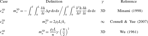
Several approximations of the added mass coefficient
 $c_{m}$
are derived in appendix B (table 3). The effect of the choice of
 $c_{m}$
on the final stability threshold turns out not to be significant. In the 3D context, we hereafter use
 $m_{a}=m_{a}^{3D}$
(B 6), which is a function of both
 $k_{y}$
and
 $k_{x}$
. We consider the mode which is a travelling wave in the streamwise
 $y$
-direction and a standing wave in the spanwise
 $x$
-direction, given by
 ${\it\zeta}=A\text{e}^{\text{i}(k_{y}y-{\it\omega}t)}\cos (k_{x}x)$
following Newman & Karniadakis (Reference Newman and Karniadakis1997), who investigated the flexible cable response using periodic solutions of a vibrating string, where
 $k_{y}$
is the streamwise wavenumber, and
 ${\it\omega}={\it\omega}_{3D}={\it\omega}_{r}+\text{i}{\it\omega}_{i}$
is the complex frequency.
Using this mode in (4.4), we obtain the dispersion relation
 $$\begin{eqnarray}\displaystyle ({\it\mu}+c_{m}){\it\omega}_{3D}^{2}+(c_{m}-1.3\mathit{Re}_{L}^{-1/2})k_{y}^{2}-(1.3{\it\nu}_{s}\mathit{Re}_{L}^{-1/2})k_{x}^{2}-2c_{m}k_{y}{\it\omega}_{3D}=0. & & \displaystyle\end{eqnarray}$$
In 3D, the new term in (4.6), the spanwise tension
 $-(1.3{\it\nu}_{s}\mathit{Re}_{L}^{-1/2})k_{x}^{2}$
, is stabilizing. From (4.6), the modal frequency is found to be
 $$\begin{eqnarray}\displaystyle {\it\omega}_{3D}^{\pm }=\frac{c_{m}k_{y}}{{\it\mu}+c_{m}}[1\pm \mathscr{P}_{3D}(k_{x},k_{y};{\it\mu})^{1/2}], & & \displaystyle\end{eqnarray}$$
where
 $P=\mathscr{P}_{3D}(k_{x},k_{y};{\it\mu})=[-{\it\mu}c_{m}k_{y}^{2}+({\it\mu}+c_{m})(\mathscr{A}(k_{x})+\mathscr{B}(k_{y}))](c_{m}k_{y})^{-2}$
,
 $\mathscr{B}(k_{y})=1.3\mathit{Re}_{L}^{-1/2}k_{y}^{2}$
, and
 $\mathscr{A}(k_{x})=1.3{\it\nu}_{s}\mathit{Re}_{L}^{-1/2}k_{x}^{2}$
. Instability occurs when
 $$\begin{eqnarray}\displaystyle \mathscr{P}_{3D}(k_{x},k_{y};{\it\mu})\leqslant 0,\quad {\it\mu}\geqslant {\it\mu}_{cr}=\frac{c_{m}\mathscr{K}_{3D}}{c_{m}k_{y}^{2}-\mathscr{A}(k_{x})+\mathscr{B}(k_{y})}. & & \displaystyle\end{eqnarray}$$
Consistent with the inviscid flow assumption, (4.7) is invariant to complex conjugation. For motions in the streamwise direction only,
 $k_{x}=\mathscr{A}=0$
, and (4.7) reduces to that for 2D in CY. From (4.7),
 ${\it\omega}_{3D}$
is real when
 $P>0$
, and the instability condition (4.8) is first met when
 $P=0$
. A flapping instability is realized when
 ${\it\mu}$
exceeds a certain critical value
 ${\it\mu}_{cr}$
, corresponding to
 $P\leqslant 0$
, yielding complex
 ${\it\omega}_{3D}$
for real
 $k_{x},k_{y}$
, with imaginary part
 $$\begin{eqnarray}\displaystyle {\it\omega}_{3D}^{i}=(-\mathscr{P}_{3D}(k_{x},k_{y};{\it\mu}))^{1/2}\leqslant {\it\omega}_{2D}^{i}=(-\mathscr{P}_{2D}(k_{y};{\it\mu}))^{1/2}, & & \displaystyle\end{eqnarray}$$
where
 $\mathscr{P}_{2D}=-[{\it\mu}c_{m}+({\it\mu}+c_{m})B(k_{y})]c_{m}^{-2}$
. Equation (4.8) is the condition for the onset of 3D flapping instability obtained with
 ${\it\omega}_{r}^{\pm }\neq 0$
and
 ${\it\omega}_{i}>0$
. For different values of
 $k_{x}L$
, we evaluate the critical mass ratio
 ${\it\mu}_{cr}$
, (4.8), and observe that 3D (
 $k_{x}>0$
) modes are more stable than 2D (
 $k_{x}0=0$
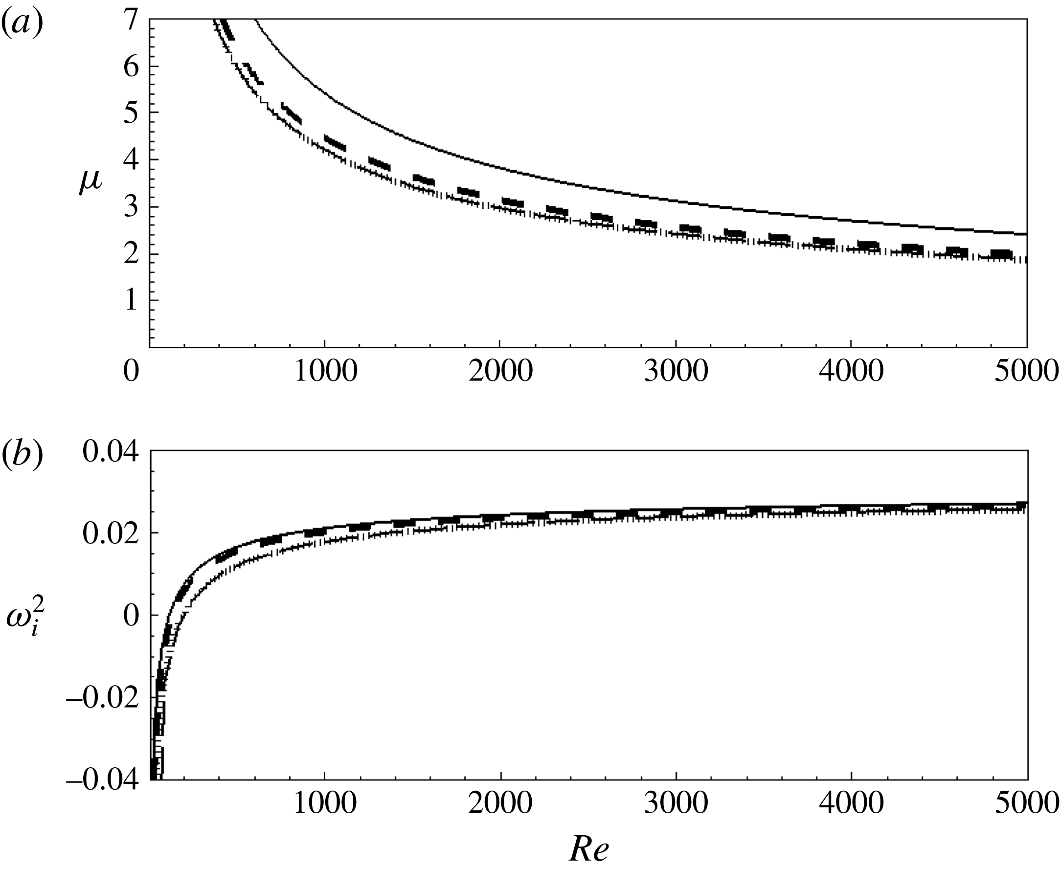
) modes. Figure 3 plots respectively the critical mass ratio
 ${\it\mu}_{cr}$
and the instability growth rate
 ${\it\omega}_{i}^{2}$
as functions of
 $\mathit{Re}_{L}$
for different
 $k_{x}L$
. Generally, the stability threshold is lower for decreasing
 $k_{x}L$
, with the results for very long spanwise variations (say,
 $k_{x}L=0.2$
) approaching that of the 2D case. The effect of Reynolds number is important for relatively smaller values of
 $\mathit{Re}_{L}$
and becomes insensitive for
 $\mathit{Re}_{L}\gtrsim 1000$
.
(a) Critical mass ratio
 ${\it\mu}_{cr}$
from (4.8), and (b) instability growth rate
 ${\it\omega}_{i}^{2}=-\mathscr{P}$
from (4.9); with
 ${\it\nu}_{s}=0.3$
; versus Reynolds number
 $\mathit{Re}_{L}$
, for
 $k_{x}L=0.2$
(——),
 $k_{x}L=0.5$
(– – –),
 $k_{x}L=1.0$
(
 $\cdots \cdots$
) and 2D (–
 $\cdot$
–).

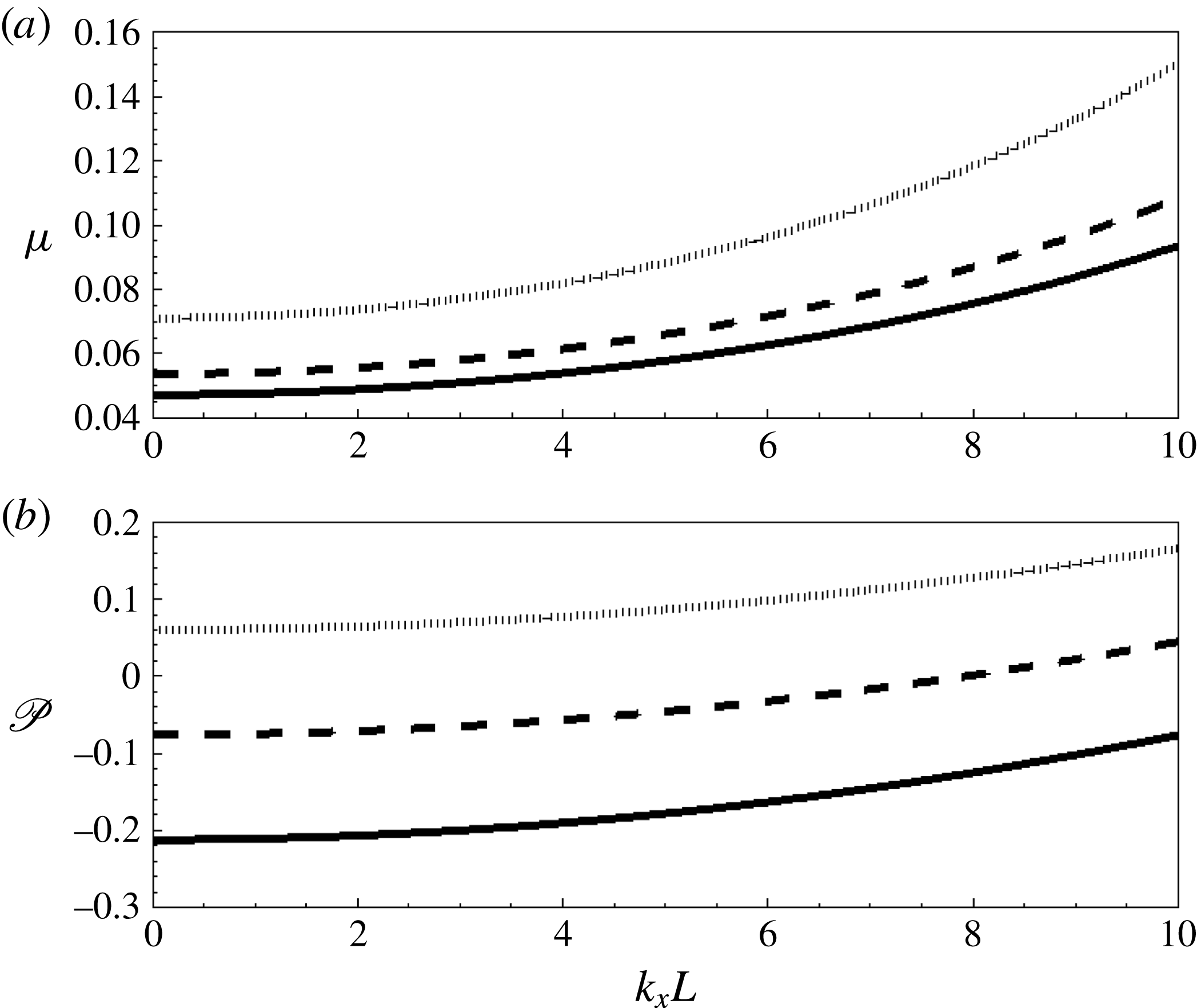
Figure 4 plots the 3D stability limit in the
 ${\it\mu}$
–
 $k_{x}$
plane for a range of
 $Re_{L}$
and in the
 $P$
–
 $k_{x}$
plane from (4.8), for a range of
 ${\it\mu}$
. Note that when the 3D approximation is taken into account,
 $c_{m}^{3D}$
lowers the stable domain as observed by Argentina & Mahadevan (Reference Argentina and Mahadevan2005), but the overall qualitative behaviour is not affected. The critical mass ratios
 ${\it\mu}_{cr}$
corresponding to
 $P=0$
in figure 4(a) show increased stability with increasing
 $k_{x}$
. From
 $\mathscr{A}(k_{x})$
, we note that the additional restoring force associated with the tension scales with
 $k_{x}^{2}$
, as shown in the figure. For
 ${\it\mu}>0.1$
, all modes with
 $k_{x}\leqslant k_{y}$
are predicted to be unstable flapping modes. Figure 4(b), shows the dependence of
 $P$
on
 $k_{x}$
when
 $P\leqslant 0$
makes the flag–fluid system unstable. Note that in all these cases, the ratio of the (real) frequency of the 3D versus 2D unstable flapping is easily given from (4.7):
 $$\begin{eqnarray}{\it\omega}_{3D}^{r}/{\it\omega}_{2D}^{r}=m_{a}^{3D}/m_{a}^{2D}.\end{eqnarray}$$
The (real) frequency of the unstable mode is thus dependent only on the (3D) added mass. A similar simple estimate of the growth rates for 3D versus 2D flapping cannot be obtained from (4.7) in the general case. For small
 $k_{x}/k_{y}$
, however, we have
 $$\begin{eqnarray}\displaystyle & \displaystyle \mathscr{P}_{3D}\sim \mathscr{P}_{2D}+(k_{x}/k_{y})^{2}1.3{\it\nu}_{s}\mathit{Re}_{L}^{-1/2}/c_{m}^{2}, & \displaystyle\end{eqnarray}$$
 $$\begin{eqnarray}\displaystyle & \displaystyle \frac{{\it\omega}_{3D}^{i}}{{\it\omega}_{2D}^{i}}\sim 1-(k_{x}/k_{y})^{2}1.3{\it\nu}_{s}\mathit{Re}_{L}^{-1/2}/(c_{m}\mathscr{P}_{2D}). & \displaystyle\end{eqnarray}$$
(a) Critical mass ratio
 ${\it\mu}$
versus cross-stream wavenumber
 $k_{x}L$
, from (4.8) with
 ${\it\nu}_{s}=0.3$
; plotted for
 $\mathit{Re}_{L}=1000$
(——),
 $\mathit{Re}_{L}=800$
(– – –) and
 $\mathit{Re}_{L}=500$
(
 $\cdots \cdots$
). (b)
 $\mathscr{P}=-{\it\omega}_{i}^{2}$
versus
 $k_{x}L$
, from (4.9) with
 $\mathit{Re}_{L}=1000$
,
 ${\it\nu}_{s}=0.3$
; plotted for
 ${\it\mu}=0.025$
(
 $\cdots \cdots$
),
 ${\it\mu}=0.075$
(– – –) and
 ${\it\mu}=0.125$
(——).

In summary, the 3D effect on stability is governed by
 $\mathscr{P}_{3D}=[-{\it\mu}c_{m}k_{y}^{2}+({\it\mu}+c_{m})(\mathscr{A}(k_{x})+\mathscr{B}(k_{y}))](c_{m}k_{y})^{-2}$
, versus
 $\mathscr{P}_{2D}=[-{\it\mu}c_{m}k_{y}^{2}+({\it\mu}+c_{m})\mathscr{B}(k_{y})](c_{m}k_{y})^{-2}$
in 2D (instability obtains when
 $\mathscr{P}_{3D}$
,
 $\mathscr{P}_{2D}<0$
). In contrast to
 $\mathscr{P}_{2D}$
,
 $\mathscr{P}_{3D}$
contains the additional term,
 $\mathscr{A}(k_{x})=1.3{\it\nu}_{s}\mathit{Re}_{L}^{-1/2}k_{x}^{2}$
, which is positive-definite, and the 3D problem is more stable for all
 $k_{x}>0$
.
5. Numerical results
We perform a targeted set of FSDS3D simulations to investigate the NL coupled dynamics of the flag. Guided by § 4, we consider a range of 3D (periodic) spanwise motions given by
 ${\it\gamma}=S/L=1,2,\ldots ,6$
for three different values of
 ${\it\mu}=0.025,0.075,0.125$
. For specificity, for most of the simulations, we fix the physical parameters
 $K_{B}=0.0001$
,
 ${\it\nu}_{s}=0.3$
and
 $\mathit{Re}_{L}=1000$
. This choice of
 $\mathit{Re}_{L}$
is mainly constrained by the direct numerical simulation computational cost of FSDS3D (although we do obtain some indication of insensitivity to variations of
 $\mathit{Re}_{L}$
around this value, appendix A.1). From LSA (cf. figure 3), the linear instability is also known to not change appreciably beyond Reynolds number
 ${\sim}1000$
.
Based on convergence tests in § 3 and appendix A, for all the simulation results here, the numerical parameters are chosen as: grid numbers
 $N_{x}\times N_{y}\times N_{z}=60\times 60\times 120$
; and time step
 ${\rm\Delta}t=0.001L/V$
. The simulations are typically run until the dynamics have achieved or approached a quasi-steady limit-cycle, typically before 22 convective cycles,
 $tV/L=22$
(except for a single
 ${\it\gamma}=5$
case where we ran up to
 $tV/L=36$
). To minimize transient effects, we specify initial flag displacements (and zero velocity) using the analytic spanwise standing wave (SW) normal modes (derived in appendix C) for a linearized thin elastic membrane subject to clamped–free boundary conditions, assuming negligible bending rigidity and Lagrangian fluid forcing. For simplicity, we include only the first chordwise
 $m=1$
term:
 $$\begin{eqnarray}\displaystyle {\it\zeta}(x,y,0)=\mathop{\sum }_{n}^{N}\text{J}_{n}({\it\alpha}_{n,1}(1-y))(\mathscr{A}_{n}\cos (2{\rm\pi}nLx/S)+\mathscr{B}_{n}\sin (2{\rm\pi}nLx/S)). & & \displaystyle\end{eqnarray}$$
To help elucidate the (expected) interactions among multiple spanwise modes in the NL evolution, we choose a finite (but relatively small, to simplify the modal evolution picture) number of spanwise modes. For most of our simulations, we use
 $N=5$
spanwise SW modes with (small) initial amplitudes
 $\mathscr{A}_{n}=\mathscr{B}_{n}=0.1L$
with
 $n=1,2,\ldots ,5$
. We also conducted simulations with a different number of initial spanwise modes; the results are qualitatively similar, and the (small) quantitative differences do not change the later conclusions.
To investigate the spanwise travelling wave (TW) response as another fundamental response of the flapping fluid–flag system, we conduct a separate set of FSDS3D simulations, where, following Newman & Karniadakis (Reference Newman and Karniadakis1997) and Williamson & Govardhan (Reference Williamson and Govardhan2004), we introduce a cross-flow component
 $(U\neq 0)$
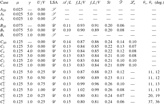
in the uniform fluid inflow. Table 1 lists the representative FSDS3D cases we conducted.
Representative FSDS3D simulations covering a range of
 ${\it\mu}$
and
 ${\it\gamma}$
, with
 $\mathit{Re}_{L}=1000$
,
 $K_{B}=0.0001$
, and
 ${\it\nu}_{s}=0.3$
. Case subscripts correspond to flag 3D parameter
 ${\it\gamma}$
. For comparison, results from the 2D case of CY are also included. Here
 $U/V$
is the strength of the cross-flow;
 $\mathscr{S}$
and
 $\mathscr{U}$
represent stable and unstable regimes according to the LSA. For the FSDS3D unstable flapping cases, limit-cycle values (obtained at
 $tV/L=22$
, except for
 $C_{5}$
at
 $tV/L=36$
) are:
 $f_{s}L/V$
, the flag flapping frequency (of the TE flag displacement);
 $f_{v}L/V$
, the vortex shedding frequency (from the wake longitudinal velocity at
 $y=2L$
,
 $z=L/4$
);
 $\mathscr{A}/L$
, the maximum TE amplitude;
 $St=f_{s}2\mathscr{A}/V$
, the flag flapping Strouhal number;
 $\bar{\mathscr{D}}$
, the time-averaged drag coefficient on the flag;
 $\mathscr{L}_{a}$
, the amplitude of the lift coefficient on the flag. For TW limit-cycle:
 ${\it\theta}_{s}$
, the angle of the TW crest along the flag; and
 ${\it\theta}_{v}$
, the angle of main wake shed from the TE, both measured from the span direction.

5.1. Development of a spanwise standing wave (SW)
In the absence of cross-flow (
 $U=0$
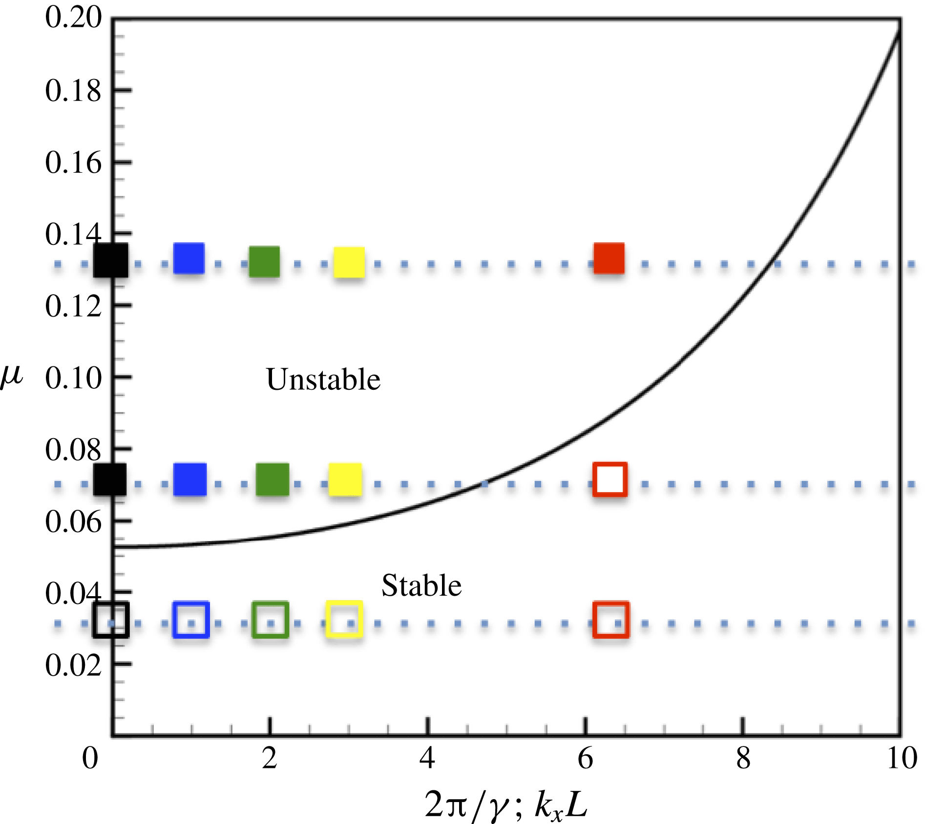
), the unstable flapping develops into SW flapping, identified as one of the fundamental responses of the flapping fluid–flag system. We confirm the LSA by examining the initial response of the fluid–flag system. For each case listed in table 1, we identify from the initial response whether the flag remains stable (the body settles to the steady straight configuration with no displacement of the TE) or becomes unstable and develops into a (3D) flapping motion. This is summarized in figure 5, in the
 ${\it\mu}$
–
 ${\it\gamma}$
parameter space, identifying two distinct regimes of response for all the cases (
 $U=0$
) in table 1. We observe that for the same
 ${\it\mu}$
, the flag becomes stable for larger
 $2{\rm\pi}/{\it\gamma}$
(shorter span); and for a specific
 $2{\rm\pi}/{\it\gamma}$
the flag becomes unstable for larger
 ${\it\mu}$
. For comparison, the
 ${\it\mu}$
–
 $k_{x}L$
stability result from LSA (4.9) is also plotted, which predicts the initial FSDS3D (in)stability.
Regime map of initial stability indication of stable (empty symbols) and unstable (filled symbols) 3D flapping, with
 $\mathit{Re}_{L}=1000$
,
 $K_{B}=0.0001$
and
 ${\it\nu}_{s}=0.3$
; for
 ${\it\mu}=0.025$
, 0.075, 0.125, obtained from FSDS3D for select 2D (black square), and 3D cases with
 ${\it\gamma}=5.0$
(blue square),
 ${\it\gamma}=3.0$
(yellow square),
 ${\it\gamma}=2.0$
(green square) and
 ${\it\gamma}=1.0$
(red square). Also plotted is the LSA prediction (4.8) (black line) (in terms of
 ${\it\mu}$
–
 $k_{x}L$
).

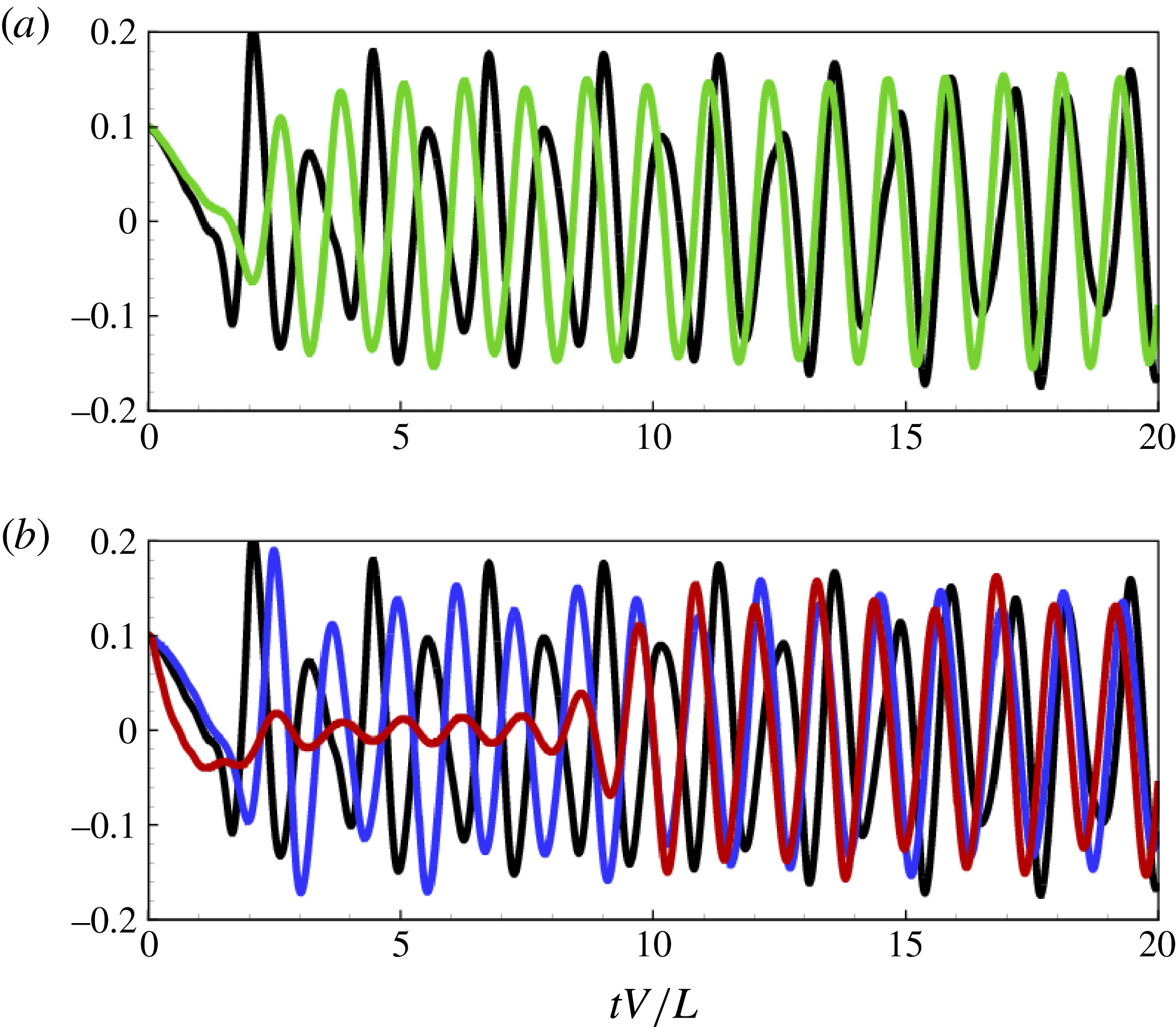
Time histories of the TE flag displacement at the spanwise antinode,
 ${\it\zeta}={\it\zeta}(x_{a},L,t)$
, for cases: (a)
 $C_{2D}$
(black line),
 $C_{2}$
(green line); (b)
 $C_{2D}$
(black line),
 $C_{5}$
(blue line),
 $C_{1}$
(red line).

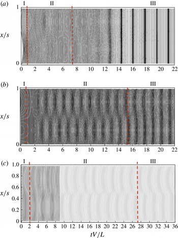
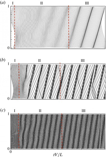
Waterfall plot of TE displacement
 ${\it\zeta}={\it\zeta}(x,L,t)$
for cases: (a)
 $C_{1}$
; (b)
 $C_{2}$
; (c)
 $C_{5}$
. Note that for
 $C_{5}$
it is plotted to time horizon
 $tV/L=36$
.

Time histories of modal amplitude
 $|{\it\zeta}_{n}(t)|$
for spanwise SW modes
 $n=0$
(black line), 1 (red line), 2 (blue line), 3 (green line) for: (a)
 $C_{1}$
; (b)
 $C_{2}$
; (c)
 $C_{5}$
. Note that for
 $C_{5}$
it is plotted to time horizon
 $tV/L=36$
.

For NL evolution, we select three unstable 3D cases,
 $C_{5}$
,
 $C_{2}$
and
 $C_{1}$
, to investigate details of the development of the spanwise standing wave (SW) flapping mode. Figure 6 plots the time histories of the TE flag displacement
 ${\it\zeta}={\it\zeta}(x_{a},y=L,t)$
, at the spanwise antinode
 $x=x_{a}$
, for
 $C_{1}$
,
 $C_{2}$
,
 $C_{5}$
, compared to the 2D case,
 $C_{2D}$
, all unstable to flapping. To depict the spanwise features, figure 7 shows the corresponding time histories of the spanwise TE flag displacement
 ${\it\zeta}(x,L,t)$
. To visualize the spanwise development, we plot
 ${\it\zeta}(x,L,t)$
in a two-dimensional waterfall plot, where
 ${\it\zeta}(x,L,t_{i})$
at successive time
 $t_{i}$
is plotted at
 $t_{i}V/L+c{\it\zeta}(x,L,t_{i})$
.
These plots of the flag TE displacements for different
 ${\it\gamma}$
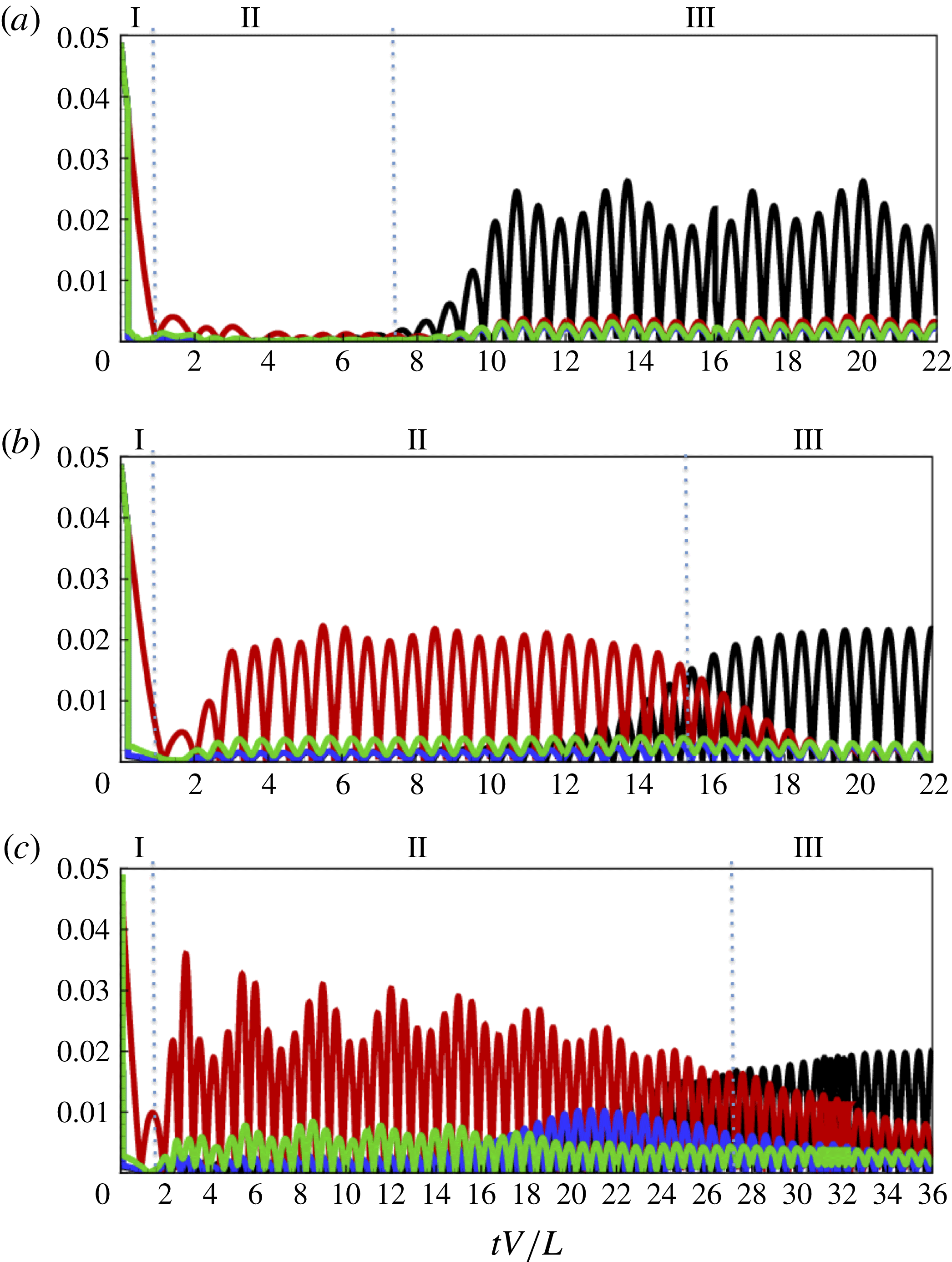
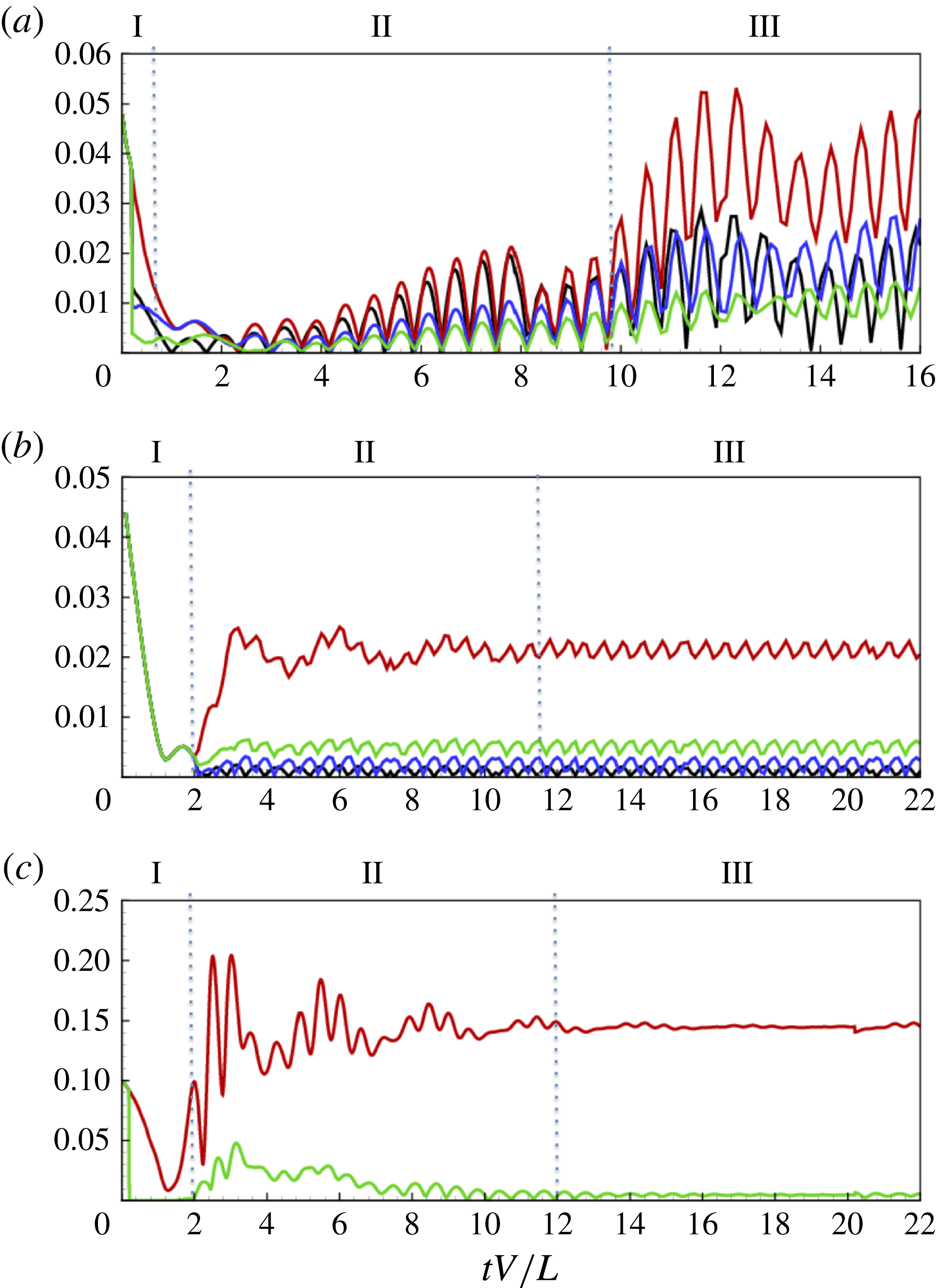
reveal three qualitative, somewhat distinct, phases (hereafter phases I, II and III), in the nonlinear evolution. The initial phase, phase I, is characterized by the initial growth of the unstable flapping modes with the initial condition (with
 $N=5$
in (5.1),
 $C_{1}$
,
 $C_{2}$
,
 $C_{5}$
contains initially 1, unstable SW modes respectively according to LSA), generally dominated by the most unstable fundamental mode. The duration of this unstable growth phase is longer for smaller values of
 ${\it\gamma}$
, which might be expected from LSA, since the growth rate for the fundamental mode for a given flag decreases with
 ${\it\gamma}$
. As the NL evolution continues, we enter phase II which is characterized by the presence and NL interactions of multiple unstable modes (including the 2D mode). Finally, after some time, the flag motion tends towards phase III where the dynamics is a quasi-steady limit cycle characterized by a single (most) dominating mode, which in the SW case corresponds to (almost) 2D flapping (these are clearly seen in the waterfall plots in figure 7). In contrast to phase I, the 2D quasi-steady flapping phase III is reached earlier for smaller
 ${\it\gamma}$
. This can be qualitatively explained, since, relative to the 2D mode, the instability of the most unstable 3D mode for a given flag is weaker for smaller
 ${\it\gamma}$
.
A more quantitative picture of the three evolution phases and the 3D modal dynamics can be obtained by considering the evolution of the spanwise SW modal amplitudes. Writing the TE displacement as
 ${\it\zeta}(x,L,t)=\text{Re}\sum _{n}{\it\zeta}_{n}(t)\exp \text{i}n2{\rm\pi}x/S$
, figure 8 plots the time histories of
 $|{\it\zeta}_{n}(t)|$
,
 $n=0,1,2,3$
for
 $C_{1}$
,
 $C_{2}$
,
 $C_{5}$
. The evolutions (after the initial transients associated with the startup of the flow) show the early unstable growth phase I, most clearly seen in
 $C_{2}$
for all three spanwise modes
 $n=1,2,3$
plotted, dominated by
 $n=1$
. Phase II can be identified with the growth of the 2D
 $n=0$
mode. This occurs later for smaller
 ${\it\gamma}$
, which suggests that the energy of the 2D mode comes from the SW modes through NL interactions and not (initially at least) from the mean flow. Phase III is the quasi-steady response dominated by the (most unstable) 2D mode, in competition with the SW modes. As explained earlier, this is reached earlier for smaller
 ${\it\gamma}$
(at
 $tV/L\approx 10$
, 18 and 36 for
 $C_{1}$
,
 $C_{2}$
and
 $C_{5}$
respectively) where the available unstable SW modes are weaker (and fewer).
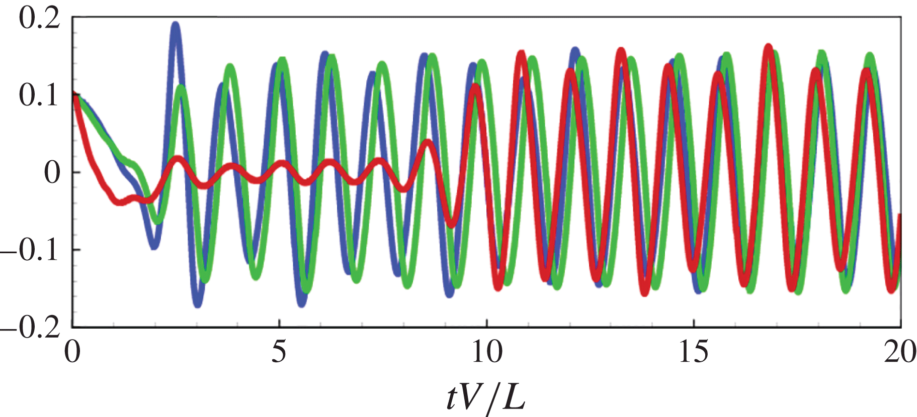
Time histories of the flag: (a) drag coefficient
 $\mathscr{D}=F_{D}/(0.5{\it\rho}_{f}V^{2}SL)$
; (b) lift coefficient
 $\mathscr{L}_{a}=F_{L}/(0.5{\it\rho}_{f}V^{2}SL)$
; (c) total energy
 $E^{T}/({\it\rho}_{f}V^{2}LS)$
for:
 $C_{1}$
(red line);
 $C_{2}$
(green line);
 $C_{5}$
(blue line).

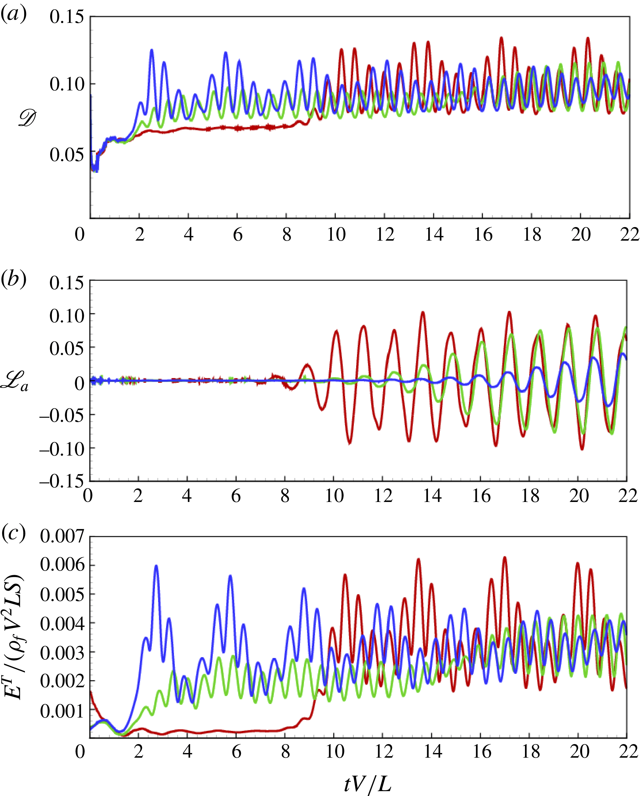
Figure 9(a,b) plots the time histories of the instantaneous drag coefficient
 $\mathscr{D}\equiv F_{D}/(0.5{\it\rho}_{f}V^{2}SL)$
and lift coefficient
 $\mathscr{L}_{a}\equiv F_{L}/(0.5{\it\rho}_{f}V^{2}SL)$
, where
 $F_{D}$
,
 $F_{L}$
are respectively the total drag and lift force on the flag. The behaviour of
 $\mathscr{D}$
and
 $\mathscr{L}_{a}$
is qualitatively different.
For
 $\mathscr{D}$
, the mean drag
 $\overline{\mathscr{D}}$
increases with the (total) flag response, indicated, e.g. by the TE antinode displacement (cf. figure 6). This increase is somewhat monotonic, eventually reaching a quasi-steady asymptotic value. This takes longer for smaller
 ${\it\gamma}$
, and in the
 $C_{1}$
case, it is not reached until Phase III. For later time, say
 $tV/L\gtrsim 10$
,
 $\overline{\mathscr{D}}$
is almost the same for the three cases, and perhaps surprisingly so for
 $C_{2}$
and
 $C_{5}$
, since this is before the quasi-2D phase III. This suggests that the total (mean squared) motion/displacement of the flag is reached in Phase II for
 $C_{2}$
and
 $C_{5}$
and remains relatively unchanged transitioning into Phase III. This is supported by looking at the evolution of the total energy of the flag motion (figure 9
c). The transition to Phase III involves a substantial gain in flag energy for
 $C_{1}$
but not for
 $C_{2}$
,
 $C_{5}$
, suggesting different fluid–structure energy transfer mechanisms between the former and the latter cases in Phases II and III, yet reaching the same asymptotic level for
 $\overline{\mathscr{D}}$
governed by the essentially 2D dynamics.
By symmetry consideration, there is no lift for SW flapping, and
 $\mathscr{L}_{a}$
essentially reflects the presence of the 2D flapping mode. Thus figure 9(b) qualitatively resembles
 $|{\it\zeta}_{0}(t)|$
in figure 8 for all three cases;
 $\mathscr{L}_{a}$
is negligible until the development of the 2D mode. Since this occurs earlier for smaller
 ${\it\gamma}$
, the lift is developed more rapidly for small
 ${\it\gamma}$
.
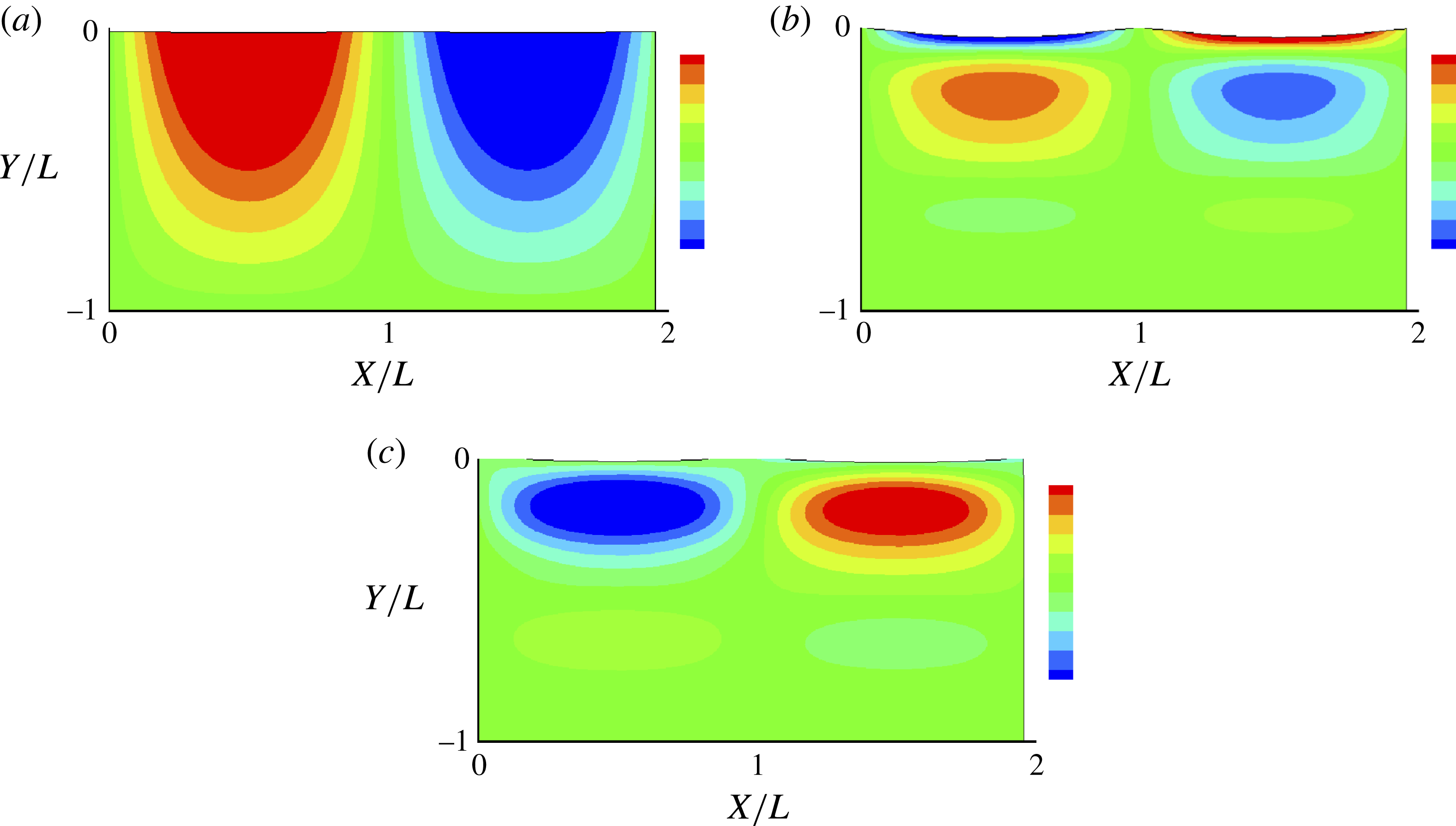
To show the 3D picture of the flag displacements, we plot contours of
 ${\it\zeta}(x,y,t)$
in figure 10 for
 $C_{2}$
(plots of other cases can be found in Banerjee Reference Banerjee2013), at three representative time instants
 $tV/L=2,6,20$
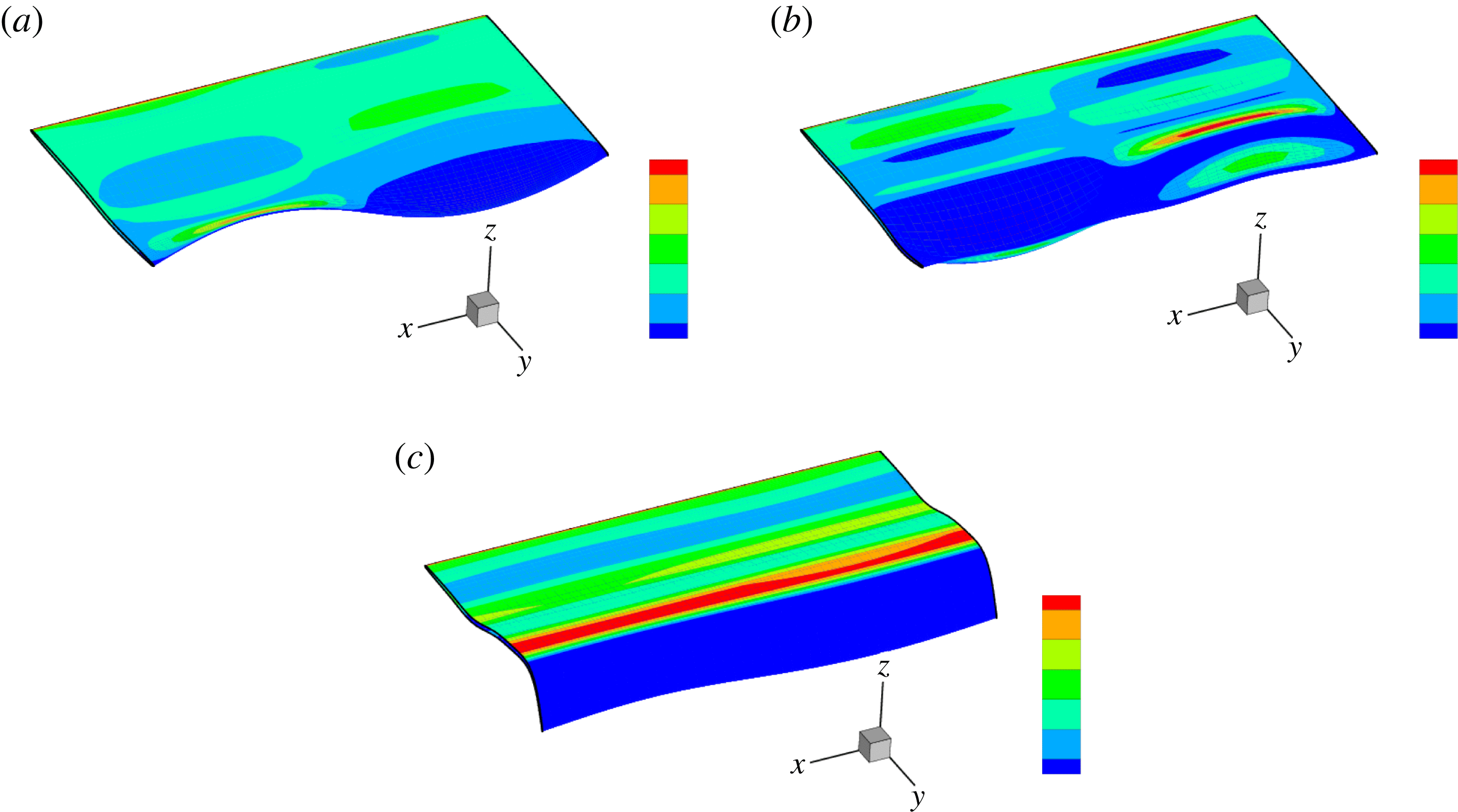
, within phases I, II and III respectively for this case. The contrast between flag displacements dominated by the most unstable 3D fundamental mode in phases I and II, and the almost 2D motion (especially near the TE) in phase III is evident. Figure 11 plots corresponding 3D snapshots showing the flag displacements, with contours of the pressure jump
 ${\rm\Delta}p$
across the flag plotted on the displaced flag surface. As expected,
 ${\rm\Delta}p$
is closely correlated with
 ${\it\zeta}$
, which helps depict the motion features. Together, these features at the three different time instants are characteristic of a 3D fundamental unstable SW mode, multiple SW interacting modes, and a dominant almost 2D mode respectively for phases I, II and III. Movies of figures 10 and 11 evolving in time (showing clearly the spanwise constant or SW motion modulated along the chord as a travelling wave) for
 $C_{1}$
,
 $C_{2}$
,
 $C_{5}$
are available at http://dx.doi.org/10.1017/jfm.2015.516. The evolution we described earlier, i.e. the phase I initial unstable growth (dominated by the most unstable fundamental mode), the phase II more complex evolution (still more or less dominated by the fundamental mode for
 $C_{2}$
at
 $tV/L=6$
cf. figure 8
b), and the phase III development of the (almost) 2D motion, are all clearly seen.
Vertical flag displacement
 ${\it\zeta}(x,y,t)$
(with contours spanning
 $\pm 0.5$
standard deviations of
 ${\it\zeta}$
), at three time instants depicting the respective evolution phases for
 $C_{2}$
: (a)
 $tV/L=2.0$
; (b)
 $tV/L=6.0$
; (c)
 $tV/L=20.0$
.

3D perspective plot of
 ${\it\zeta}(x,y,t)$
with contours of the pressure jump across the flag surface
 ${\rm\Delta}p(x,y,t)$
(with contours spanning
 $\pm 0.25$
standard deviations of
 ${\rm\Delta}p$
) superposed on the displaced flag surface, at three time instants depicting the respective evolution phases for
 $C_{2}$
: (a)
 $tV/L=2.0$
; (b)
 $tV/L=6.0$
; (c)
 $tV/L=20.0$
.

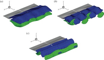
Finally, we show the vortex structure in the wake associated with the SW motion of the flag body. To highlight the 3D effects we consider separately the primary spanwise vorticity
 ${\it\omega}_{x}$
, and the secondary vorticity
 ${\it\omega}_{s}\equiv ({\it\omega}_{y}^{2}+{\it\omega}_{z}^{2})^{1/2}$
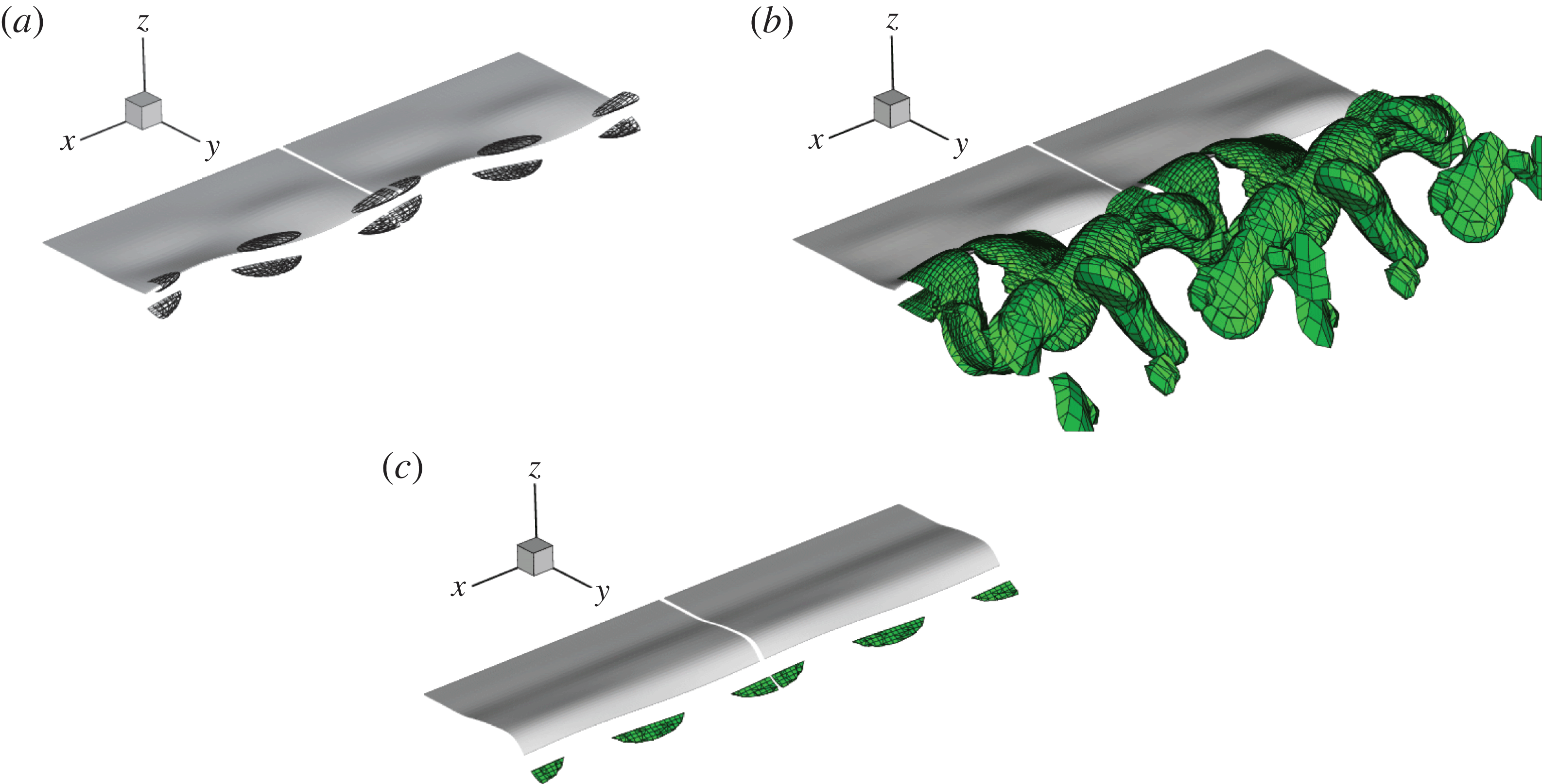
. Figures 12 and 13 plot the isosurfaces of
 ${\it\omega}_{x}$
and
 ${\it\omega}_{s}$
respectively at the three representative instants (note the different isosurface levels) for case
 $C_{2}$
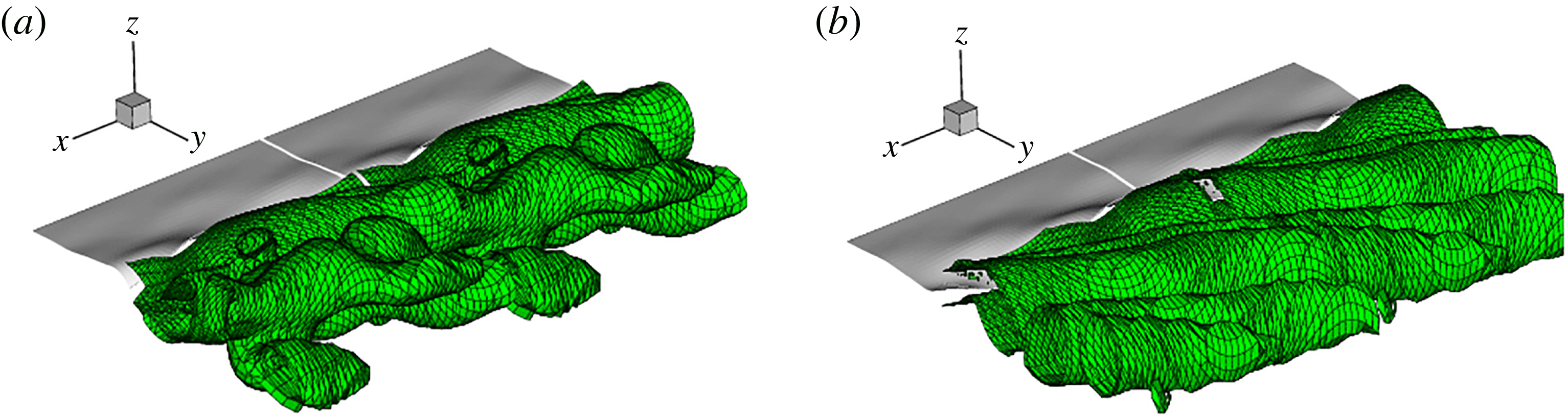
(the vortical structures for the other cases are qualitatively similar and reported in Banerjee Reference Banerjee2013). Figure 12 shows the characteristic braided split vortex (SV) structures for phase I and II associated with spanwise SW motions (e.g. Newman & Karniadakis Reference Newman and Karniadakis1997, for the case of a vibrating cylinder). The primary SV structures are more developed and complex for phase II, showing the presence of secondary SV structures. In phase III, the vortex structure approaches the classical 2D Karman vortex shedding. The qualitative picture is consistent in the
 ${\it\omega}_{s}$
isosurfaces showing that
 ${\it\omega}_{s}$
is present primarily in phase I and II, predominately in II (associated with shorter spanwise modes), and almost absent in phase III. The overall picture is that of a single primary SW mode with SV vortex in phase I, complex multiply modulated SW modes and braided SV in phase II, and almost 2D motion and spanwise uniform vortex structure in phase III.
Isosurfaces of spanwise wake vorticity
 ${\it\omega}_{x}$
for
 $C_{2}$
(from an oblique downstream perspective) at three characteristic time instants: (a–c)
 $tV/L=2.0$
, 6.0, 20.0 within phases I, II and III of the flapping evolution. The isosurfaces plotted are for negative (blue) and positive (green) values of the vorticity corresponding to
 ${\it\omega}_{x}=0.7$
, 1.2 and 1.5 for
 $tV/L=2$
, 6, 20 respectively (the maximum values in the wake at these three instants are
 $|{\it\omega}_{x}|^{max}=6.9$
, 12.1, 15.0).

Isosurfaces of the 3D wake vorticity
 $|{\it\omega}_{s}^{max}|$
(from an oblique downstream perspective) at three characteristic time instants: (a–c)
 $tV/L=2.0$
, 6.0, 20.0 within phases I, II and III of the flapping evolution. The isosurfaces plotted are for negative (blue) and positive (green) values of the vorticity corresponding to
 ${\it\omega}_{s}=0.16$
, 1.03 and 0.02 for
 $tV/L=2$
, 6, 20 respectively (the maximum values in the wake at these three instants are
 $|{\it\omega}_{s}|^{max}=1.6$
, 10.3, 0.2).

The presence of the quasi-steady limit-cycle 2D response in long-time phase III allows us to obtain quantitative measures of the dominant flag flapping motion characteristics. These are given in table 1 for all the unstable SW (
 $U=0$
) cases (note that for cases
 $C_{5}$
and
 $C_{6}$
, phase III has not been fully reached at the end of the simulation at
 $tV/L=22$
, and the values are approximate). For the TE amplitude
 $\mathscr{A}$
, for a given
 ${\it\mu}$
the values are almost the same for different
 ${\it\gamma}$
(and close to the 2D case) indicating that three-dimensionality is no longer in play in phase III. For increasing
 ${\it\mu}$
,
 $\mathscr{A}$
also increases, reflecting greater instability associated with greater mass ratio (a result reported for the 2D case, see CY). The flapping frequency of the flag
 $f_{s}L/V$
is independent of
 ${\it\gamma}$
(as expected), but also of
 ${\it\mu}$
(as in the 2D case), and (again as expected) is closely matched to the vortex shedding frequency
 $f_{v}L/V$
. Since
 $\mathscr{A}$
increases with
 ${\it\mu}$
, the combined result is that the Strouhal number of the vortex shedding
 $St=2\mathscr{A}f_{s}/V$
is lower for smaller
 ${\it\mu}$
.
For the forces on the flag, the lift and drag oscillation frequencies are close to
 $f_{s}$
and
 $2f_{s}$
respectively (cf. Michelin, Smith & Glover Reference Michelin, Smith and Glover2008). Again, the mean drag coefficient
 $\overline{\mathscr{D}}$
and amplitude of lift coefficient
 $\mathscr{L}_{a}$
are somewhat independent of
 ${\it\gamma}$
(except for the cases where phase III is not reached).
 $\mathscr{L}$
somewhat lower than for 2D.
5.2. Development of spanwise travelling waves (TW)
Although SW patterns are common in experimental situations, TW responses have been realized both in laboratory and field experiments on flexible cables, e.g. by Alexander (Reference Alexander1981) and Atta, Gharib & Hammache (Reference Atta, Gharib and Hammache1988). This is confirmed in numerical simulations by using a non-zero spanwise cross-flow
 $U\neq 0$
in the problem (Newman & Karniadakis Reference Newman and Karniadakis1997). To investigate the development of the TW mode in the flag flapping response, we follow Newman & Karniadakis (Reference Newman and Karniadakis1997) and introduce a small uniform cross-flow
 $U$
in FSDS3D (retaining the same SW initial condition (5.1)). We consider a range of
 $U/V$
, and find that, while
 $U/V$
affects the time scale of TW development, the response characteristics and amplitudes are not sensitive to the strength of (small)
 $U/V\lesssim 1$
(see table 1). Hereafter, we discuss the results for
 $U/V=0.25$
.
Time histories of the TE flag displacement at
 $x=0$
,
 ${\it\zeta}={\it\zeta}(0,L,t)$
, for cases
 $C_{1}^{U}$
(red line);
 $C_{2}^{U}$
(green line);
 $C_{5}^{U}$
(blue line).
 $U/V=0.25$
.

Figure 14 plots the time histories of the TE flag displacement at a fixed span position
 ${\it\zeta}={\it\zeta}(0,y=L,t)$
, for three 3D cases,
 $C_{1}^{U}$
,
 $C_{2}^{U}$
and
 $C_{5}^{U}$
. To show the spanwise features, figure 15 gives the TE flag displacement
 ${\it\zeta}(x,L,t)$
in a waterfall plot for the three cases. Figure 16 plots the evolution of the TW spanwise modal amplitudes
 $|{\it\zeta}_{n}(t)|$
of the TE flag displacement
 ${\it\zeta}(x,L,t)$
.
Waterfall plot of TE displacement
 ${\it\zeta}={\it\zeta}(x,L,t)$
(vertical displacement profiles
 ${\it\zeta}(x,L;t)$
shifted horizontally for successive times
 $t$
) for cases: (a)
 $C_{1}^{U}$
with
 $tV/L=[0,16]$
; (b)
 $C_{2}^{U}$
with
 $tV/L=[0,22]$
; (c)
 $C_{5}^{U}$
with
 $tV/L=[0,22]$
, all for
 $U/V=0.25$
.

As expected from LSA, the 3D cases initially develop into SW flapping (phase I). After a short transient, in the presence of cross-flow, distinct TW modes soon develop (phase II), replacing the SW flapping. A quasi-steady limit cycle (phase III) consisting mainly the fundamental spanwise TW mode (with small SW higher harmonics) follows thereafter. Comparing the TE amplitudes for the different
 ${\it\gamma}$
in figure 14 (which plots essentially the TW amplitudes except at the very initial time), and referring to the waterfall plots (figure 15) and the modal evolution (figure 16), we see that, relative to the SW cases, the (single dominant TW mode) phase III develops much earlier for all cases, and in contrast to SW, phase III takes longer to be attained for smaller
 ${\it\gamma}$
. As in the SW case, the phase III displacement amplitudes are of comparable magnitude for the three cases (see table 1).
Time histories of modal amplitudes
 $|{\it\zeta}_{n}(t)|$
for spanwise TW modes
 $n=0$
(black line), 1 (red line), 2 (blue line), 3 (green line) for (a)
 $C_{1}^{U}$
, (b)
 $C_{2}^{U}$
and (c)
 $C_{5}^{U}$
.

The general features of the TW evolution are qualitatively similar for different
 ${\it\gamma}$
. For illustration, we focus hereafter only on the intermediate
 $C_{2}^{U}$
case.
Evolution of the flag drag coefficient
 $\mathscr{D}=F_{D}/(0.5{\it\rho}_{f}V^{2}SL)$
(green line) and total energy
 $E^{T}/({\it\rho}_{f}V^{2}LS)\times 10$
(green dashed line) for
 $C_{2}^{U}$
.

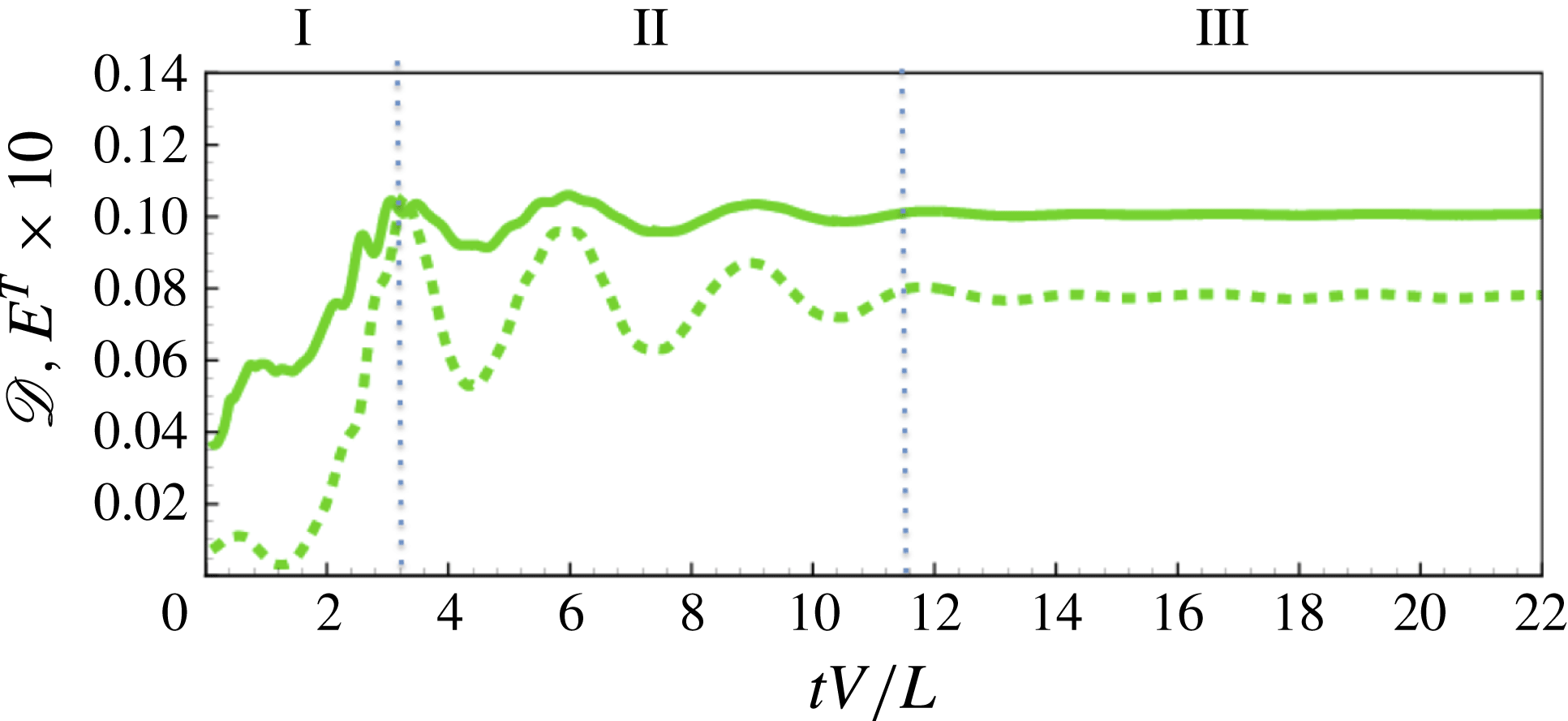
Figure 17 plots the evolution of the flag drag and total energy. In the presence of the cross-flow, the fluctuating drag is stabilized (cf. figure 9 for the SW drag), reaching a constant (instantaneous)
 $\mathscr{D}$
after a relatively short time. With development of the dominant TW mode and vanishing of the SW (and the 2D
 $|{\it\zeta}_{0}|$
),
 $\mathscr{L}_{a}$
is negligible throughout (except during phase I) and is not plotted. The evolution of the flag energy reflects that of
 $\mathscr{D}$
, and the fluctuations observed in the SW response are again absent (cf. figure 9).
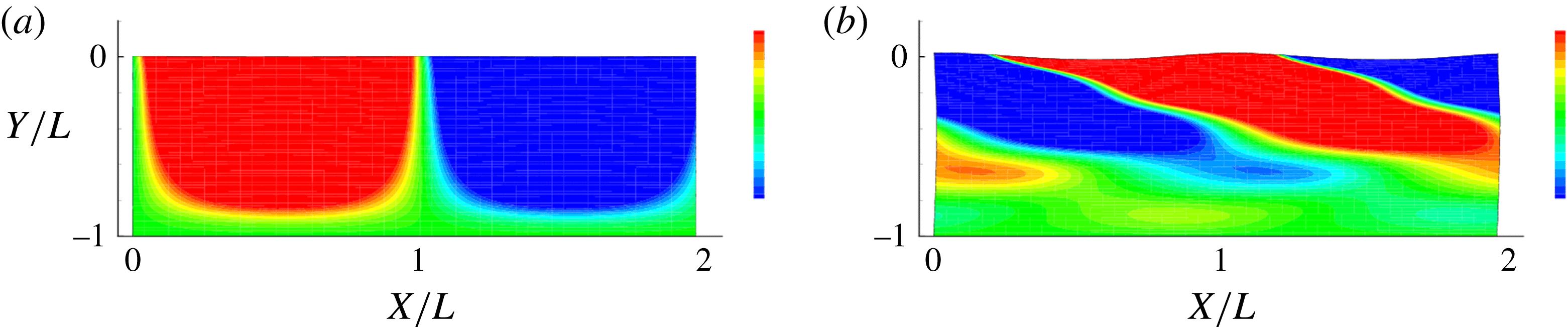
Figure 18 plots contours of vertical flag displacement
 ${\it\zeta}(x,y,t)$
at
 $tV/L=2$
(phase I) and 20 (phase III), showing the growth of the displacement from the LE (where
 ${\it\zeta}=0$
) to the TE. Figure 18 shows clearly the transition from SW-dominated phase I (figure 18
a) to the TW response (dominated by the fundamental mode) in Phase III (figure 18
b). (Movies of
 ${\it\zeta}(x,y,t)$
contour plots, as well as 3D plots of the displaced flag surface superimposed with contours of the pressure jump
 ${\rm\Delta}p$
across the flag surface for
 $C_{2}^{U}$
,
 $C_{5}^{U}$
, see supplementary data.)
Vertical flag displacement
 ${\it\zeta}(x,y,t)$
(with contours spanning
 $\pm 0.25$
standard deviations of
 ${\it\zeta}$
), at two time instants, for
 $C_{2}^{U}$
: (a)
 $tV/L=2.0$
; (b)
 $tV/L=20.0$
.

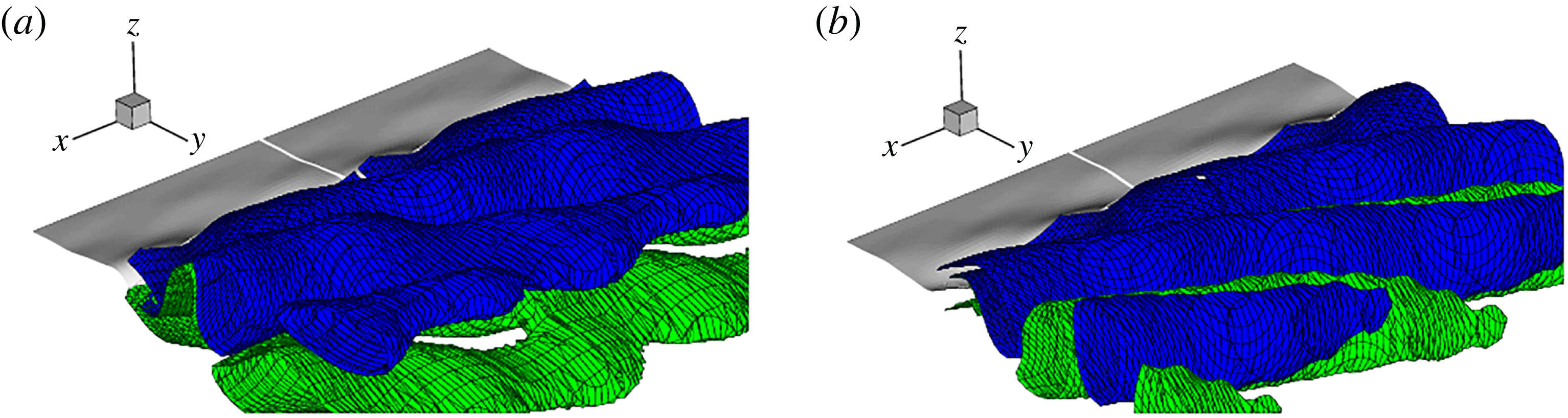
Finally, we show details of the vortex wake associated with TW. Figures 19(a) and 19(b) plot the isosurfaces of
 ${\it\omega}_{x}$
at the two instants in figure 18 respectively. The characteristic braided split vortex (SV) structures at early time are qualitatively similar to those in the SW cases associated with spanwise SW motions. At later time, the SW mode(s) disappear and the TW response develops, and we obtain continuous vortex (CV) structures shed at an oblique angle (
 ${\it\theta}_{v}$
). The CV structure is consistent with and might be expected from the near constant value of
 $\mathscr{D}$
in Phase III (figure 17). The transition from SV SW to CV TW and the persistence of the latter in phase III are consistent with the observations of Newman & Karniadakis (Reference Newman and Karniadakis1997) for flow past a cable. Figures 20(a) and 20(b) plot the isosurfaces of
 ${\it\omega}_{s}$
for TW at the two instants respectively. The attenuation of
 ${\it\omega}_{s}$
with streamwise distance is slower than in the SW case (cf. figure 13). We furthermore provide direct support and an explanation of the presence of lift in the SW case due to the 2D (zeroth) SW mode, which is absent in the TW.
The limit-cycle TW phase III response characteristics can be obtained as before. Table 1 shows limit-cycles values of interest for select cases. For the TE amplitude, we see from the
 $C_{5}^{U}$
cases that
 $\mathscr{A}/L$
is the same for different
 $U/V$
indicating that, while
 $U$
is responsible for the transition from SW to TW, it does not significantly affect the subsequent dynamics. For smaller
 ${\it\gamma}$
,
 $\mathscr{A}/L$
is somewhat larger, although the TE amplitudes are in general quite comparable for all the SW and TW cases. The variations of the flag flapping frequency
 $f_{s}$
and vortex wake frequency
 $f_{v}$
with
 ${\it\gamma}$
(and
 $U/V$
) are relatively small, and these are approximately matched, as would be expected in lock-in regime. While the responses are qualitatively different, the limit-cycle SW and TW frequencies are relatively close, although, with the TE amplitude factored in, the TW Strouhal numbers
 $St$
are generally somewhat higher. As with the SW case, the quasi-steady drag for TW is (slightly) lower for smaller
 ${\it\gamma}$
, while for comparable
 ${\it\gamma}$
,
 $\overline{D}$
is somewhat lower but of comparable magnitude to the SW drag. In contrast to the SW limit-cycle response, however, the phase III TW lift is negligible, indicative of the absence of the zeroth/2D SW mode in the final response.
Isosurfaces of spanwise wake vorticity
 ${\it\omega}_{x}$
for
 $C_{2}^{U}$
(from an oblique downstream perspective) at two characteristic time instants: (a)
 $tV/L=2.0$
, (b)
 $tV/L=20.0$
, within phases I, II and III of the flapping evolution. The isosurfaces plotted are for negative (blue) and positive (green) values of the vorticity corresponding to
 ${\it\omega}_{x}=0.7$
, 2.2 for
 $tV/L=2$
, 20 respectively (the maximum values in the wake at these three instants are
 $|{\it\omega}_{x}|^{max}=7.1$
, 22.8).

Isosurfaces of spanwise wake vorticity
 $|{\it\omega}_{s}^{max}|$
for
 $C_{2}^{U}$
(from an oblique downstream perspective) at two characteristic time instants: (a)
 $tV/L=2.0$
, (b)
 $tV/L=20.0$
, within phases I, II and III of the flapping evolution. The isosurfaces plotted are for negative (blue) and positive (green) values of the vorticity corresponding to
 ${\it\omega}_{s}=0.3$
, 1.0 for
 $tV/L=2$
, 20 respectively (the maximum values in the wake at these three instants are
 $|{\it\omega}_{s}^{max}|=3.2$
, 10.1).

Finally, for the TW response, we look at the oblique angle of the TW flag displacement
 ${\it\theta}_{s}$
, and that of the CV wake
 ${\it\theta}_{v}$
. As expected,
 ${\it\theta}_{s}\approx {\it\theta}_{v}$
(the latter value is somewhat less precise). Since the phase III response is the fundamental mode, the TW frequencies
 $f_{s,v}^{U}$
can be related to that of the 2D response
 $f_{s,v}^{2D}$
through the shedding angles
 ${\it\theta}_{s,v}$
by a simple geometric argument (cf. Williamson Reference Williamson1989) to obtain:
 $f_{s,v}^{U}\approx f_{s,v}^{2D}\cos ({\it\theta})_{s,v}$
. Using the respective values from table 1 for the
 $C_{5}^{U}$
cases, this relationship is satisfied to within 3 %, 5 %, 13 %, 17 % for
 $U/V=0.25$
, 0.5, 0.75, 1 respectively for
 $v$
(comparable values for
 $s$
), reflecting somewhat the effect of the cross-flow magnitude.
We remark finally that the choice of
 $\mathit{Re}_{L}(=1000)$
in this work is mainly constrained by the computational cost of the direct numerical simulation FSDS3D, although we do obtain some indication of insensitivity to variations of
 $\mathit{Re}_{L}$
around this value, see appendix A.1. From LSA (§ 4), the linear instability is also known to not change appreciably beyond Reynolds number
 ${\sim}1000$
. For the somewhat related problem of flow past a long cylinder, Williamson (Reference Williamson1996) found onset of 3D effects above Reynolds number based on diameter of
 $Re_{D}=UD/{\it\nu}\geqslant 150{-}300$
. We do not observe evidence of this in our simulations, and indeed obtain quasi-steady 2D responses (for SW). Using our TE amplitude of
 $2\mathscr{A}/L\sim O(0.3)$
(table 1), our corresponding double-amplitude Reynolds number
 $\mathit{Re}_{2A}$
is
 $O(300)$
, which apparently is still not large enough for the onset of this 3D effect for the present problem.
6. Conclusions
In this paper we have studied the 3D effects in terms of dimensionless spanwise wavelength (
 ${\it\gamma}$
) on the flapping dynamics of a flag in a uniform fluid flow using LSA and nonlinear FSDS3D simulations. LSA obtains that, for a given mass ratio, the stability increases with dimensionless spanwise wavelength, with the purely 2D mode being the most unstable. We perform FSDS3D considering the absence and presence respectively of (small) cross-flow
 $U/V>0$
to obtain distinct characteristic SW and TW responses. Both SW and TW responses show three temporal phases: phase I characterized by initial instability growth; phase II by multiple unstable 3D modes; and a long-time phase III response dominated by a single most unstable transverse mode corresponding to the 2D (
 $n=0$
) mode for SW, and the fundamental (
 $n=1$
) mode for TW. We present the vortex wake structures, at different phases, for SW and TW, characterized respectively by interwoven braided split vortex (SV) and oblique continuous vortex (CV) structures.
The dominant (limit-cycle) flag flapping and vortex shedding frequencies are matched. These frequencies for SW and TW are found to be related, after factoring in the shedding angle of the latter given in terms of dimensionless spanwise wavelength. The drag on the flag generally increases with the evolution, with the SW magnitude somewhat greater than that of the TW. In the presence of cross-flow, the TW lift is always negligible. For SW, the lift is small in phases I and II, but becomes significant in (quasi-2D) phase III with a magnitude comparable to that of the drag.
The present study provides useful insights into the more general dynamics of a large-span flag with continuous spectrum of spanwise modes. A main limitation of this work is the neglect of finite span with edge effects, where linear stability analysis (Eloy et al. Reference Eloy, Souilliez and Schouveiler2007) shows further increase in stability. Our numerical approach can be extended directly to include a flag of limited span with vortex shedding also along lateral edges. This is a matter of future study.
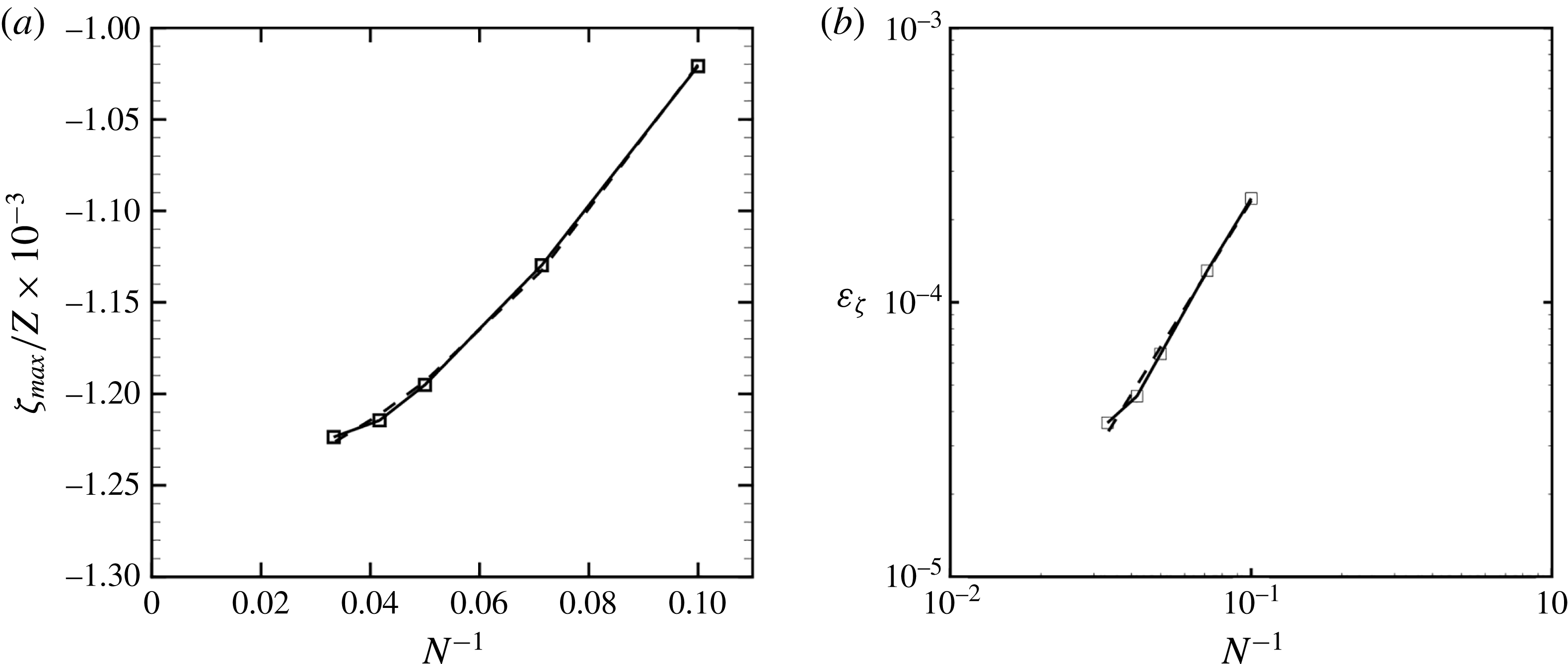
(a) Maximum steady-state displacement
 ${\it\zeta}_{max}/Z$
(–▫–) for a clamped plate under uniform load obtained using an
 $N\times N$
SDS grid with
 $N=(11,15,21,25,31)$
. A quadratic fit (– – –) of the data
 ${\it\zeta}_{max}/Z=-0.00126(1-0.14N^{-1}-17.48N^{-2})$
is plotted. (b) Error
 ${\it\varepsilon}_{{\it\zeta}}$
(–▫–) in the SDS prediction of
 ${\it\zeta}_{max}$
relative to analytical value versus
 $N^{-1}$
. The power-law fit (– – –) yields
 ${\it\varepsilon}_{{\it\zeta}}\sim N^{-1.77}$
.

Acknowledgements
This work is supported financially by the Office of Naval Research. We thank our colleagues G. Tokic and K. Hendrickson for many helpful discussions.
Supplementary movies
Supplementary movies are available at http://dx.doi.org/10.1017/jfm.2015.516.
Appendix A. Validation of the SDS solver
Our interest in this paper is to solve the flag problem (for computational stability we include low bending rigidity); however, we validate our code for the structural solver against the closed-form solution of a plate. We verify the 3D SDS using the case of a square plate, length
 $L$
, under a uniform load
 $q$
. We first compare the numerical prediction to the linearized analytical solution (Shames & Dym Reference Shames and Dym1985) for the maximum displacement (at the plate centre) of a fully clamped plate:
 $$\begin{eqnarray}{\it\zeta}_{max}/Z=0.00126,\quad Z\equiv qL^{4}\left[\frac{Eh^{3}}{12(1-{\it\nu}_{s}^{2})}\right]^{-1}.\end{eqnarray}$$
This problem is solved with SDS on
 $N\times N$
grids with successively increasing
 $N$
to examine the convergence with grid spacing. A plot of
 ${\it\zeta}_{max}/Z$
against
 $N^{-1}$
is given in figure 21(a), where a quadratic fit gives an intercept of
 ${\it\zeta}_{max}/Z=0.00126$
, almost exactly the linearized value in (A 1). The error
 ${\it\varepsilon}_{{\it\zeta}}$
from the theoretical value versus
 $N^{-1}$
is plotted in figure 21(b), which yields the fit of
 ${\it\varepsilon}_{{\it\zeta}}\sim N^{-1.77}$
, indicating the (approximate) second-order convergence with grid spacing expected. If the plate is simply supported, the linearized analytical solution for the natural frequency of the first mode is (Shames & Dym Reference Shames and Dym1985)
 $$\begin{eqnarray}{\it\omega}_{1}/{\it\Omega}=19.9L^{-2},\quad {\it\Omega}\equiv \left[\frac{Eh^{3}}{12(1-{\it\nu}_{s}^{2}){\it\rho}h}\right]^{1/2}.\end{eqnarray}$$
The prediction from SDS using
 $N=25$
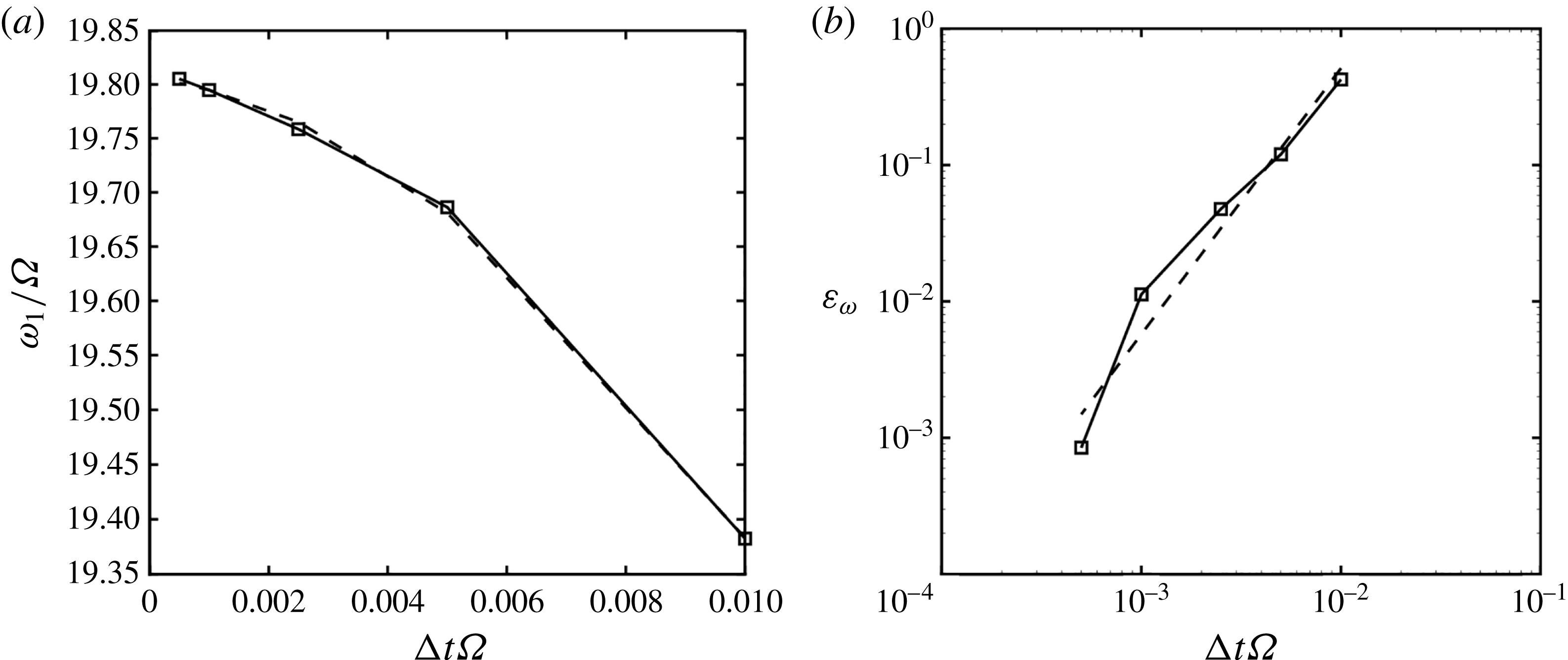
and different integration time steps
 ${\rm\Delta}t$
is given in figure 22(a), where a quadratic fit gives an intercept of
 ${\it\omega}_{1}/{\it\Omega}=19.81$
, a 0.45 % difference from the linear solution. The error
 ${\it\varepsilon}_{{\it\omega}}$
from the theoretical value versus
 ${\rm\Delta}t{\it\Omega}$
plotted in figure 22(b) yields a fit of
 ${\it\varepsilon}_{{\it\omega}}\sim ({\rm\Delta}t{\it\Omega})^{1.95}$
, consistent with the expected second-order convergence with time step. To evaluate the nonlinear prediction of SDS, we compare to the semi-analytical nonlinear solution of Kirby & Yosibash (Reference Kirby and Yosibash2004) for the static displacement of the square plate. For
 $L/h=20$
and
 ${\it\nu}_{s}=0.3$
with uniform load
 $q=26.15[Eh^{3}/(12(1-{\it\nu}_{s}^{2})L^{3})]$
, they found a maximum displacement of
 ${\it\zeta}_{max}/Z=0.02615$
. With such displacement, the magnitude of the restoring tension associated with the nonlinearity is
 ${\sim}16\,\%$
, the magnitude of the bending restoring force for the
 $kL=2{\rm\pi}$
mode. With these parameters in (A 1), the linearized solution differs from the nonlinear value by
 ${\sim}14\,\%$
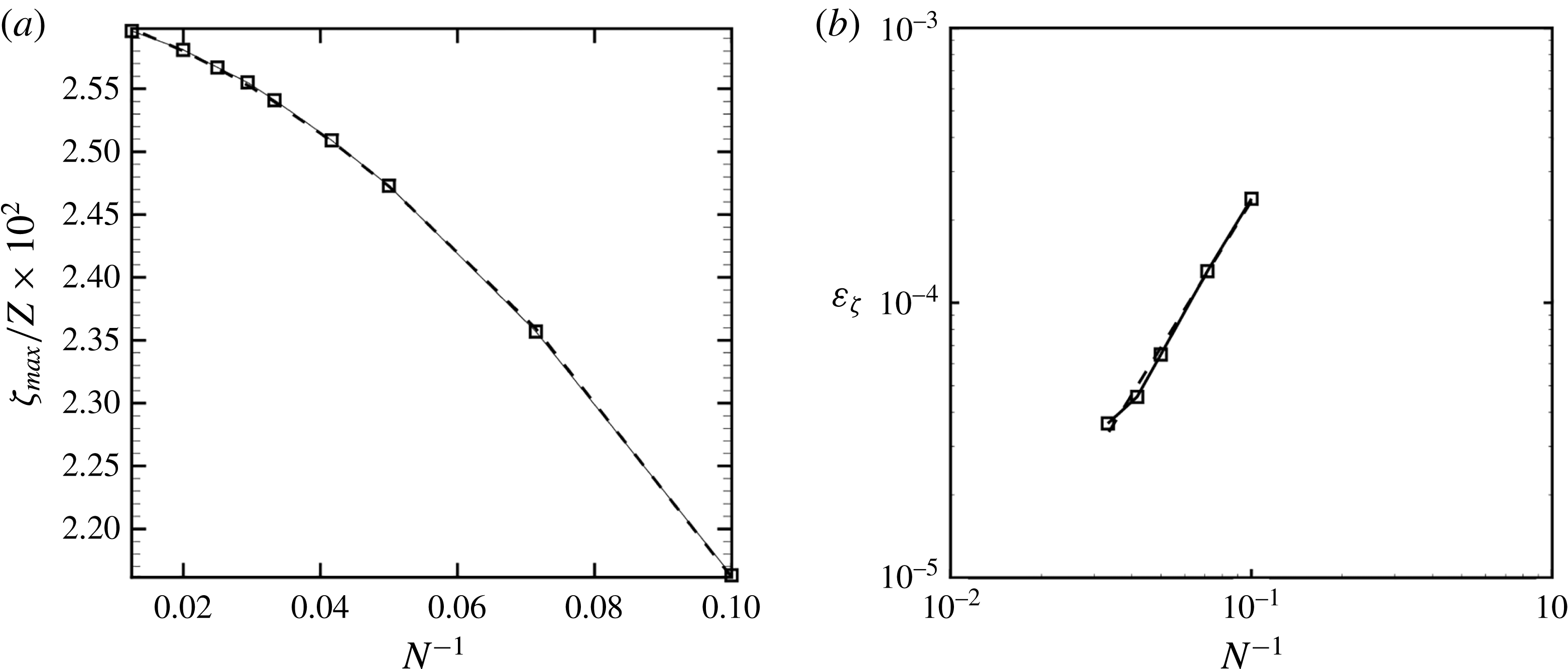
. The SDS prediction of
 ${\it\zeta}_{max}$
using an
 $N\times N$
grid is given in figure 23(a). A quadratic fit gives a predicted value for large
 $N$
of
 ${\it\zeta}_{max}/Z=0.02619$
, a 0.15 % difference from that given by Kirby & Yosibash (Reference Kirby and Yosibash2004). A similar fit as in figure 21 yields an error convergence rate of
 ${\it\varepsilon}_{{\it\zeta}}\sim ({\rm\Delta}x/L)^{1.46}$
, showing some decrease in the convergence with grid refinement associated with the nonlinear stretching terms in (3.4). We provide a final demonstration of SDS for the highly nonlinear problem of a thin membrane with a simply supported edge released from horizontal under the influence of gravity. Using a
 $N=50$
grid and structural parameters of
 $(Eh^{3}/(12(1-{\it\nu}_{s}^{2})))/[{\it\rho}hgL^{3}]=0.01$
,
 $(Eh/(1-{\it\nu}_{s}^{2}))/[{\it\rho}hgL]=100$
,
 ${\it\nu}_{s}=0.3$
, and Kelvin–Voight structural damping of
 $G=0.001$
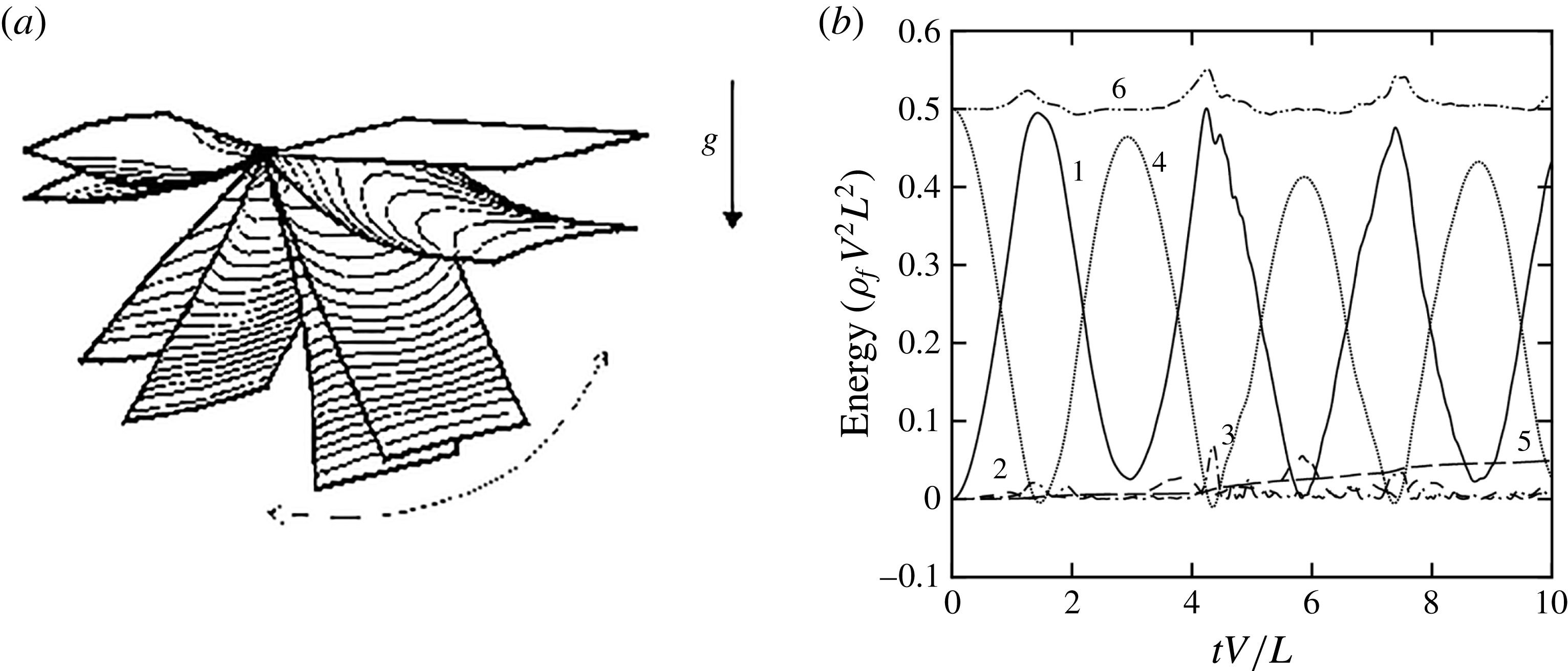
, a SDS simulation is performed. A series of snapshots of the swinging membrane is shown in figure 24(a). The contours of extensional strain indicate the increase in tension at the bottom of the swing. The 3D effects are evident in the curvature of the end and the variation of the strain toward the edges. The energy budget for the simulation is given in figure 24(b), showing satisfactory conservation of the total energy.
(a) Frequency
 ${\it\omega}_{1}/{\it\Omega}$
(–▫–) of the first mode of the simply supported square plate using
 ${\rm\Delta}t{\it\Omega}=(0.01,0.005,0.0025,0.001)$
. A quadratic fit (– – –) of the data
 ${\it\omega}_{1}/{\it\Omega}=19.806(1-0.39({\rm\Delta}t{\it\Omega})^{-1}-174.8({\rm\Delta}t{\it\Omega})^{-2})$
is plotted. (b) Error of the frequency (–▫–) from the
 ${\it\omega}/{\it\Omega}=19.81$
intercept with
 ${\it\varepsilon}_{{\it\omega}}\sim ({\rm\Delta}t{\it\Omega})^{1.95}$
(– – –) curve fit.

(a) Maximum steady-state displacement
 ${\it\zeta}_{max}/Z$
(–▫–) for clamped plate under uniform load with varying grid spacing in the nonlinear regime. For comparison to Kirby & Yosibash (Reference Kirby and Yosibash2004), using
 $L/h=20$
,
 ${\it\nu}_{s}=0.3$
, and
 $q[Eh^{3}/(12(1-{\it\nu}_{s}^{2})L^{3})]^{-1}=26.15$
, on an
 $N\times N$
grid with
 $N=(11,15,21,25,31,35,41,51,81)$
. A quadratic fit (– – –) of the data
 ${\it\zeta}_{max}/Z=-0.02619(1-0.4903N^{-1}-12.564N^{-2})$
is plotted. (b) Error from the
 ${\it\zeta}_{max}/Z=0.02619$
(–▫–) intercept with
 ${\it\varepsilon}_{{\it\zeta}}\sim (N)^{-1.46}$
(– – –) curve fit.

(a) Series of snapshots of the swinging membrane with contours of extensional strain, showing increase in strain at the bottom of the swing, as well as the spanwise variation of the strain. (b) Energy budget of the nonlinear swinging membrane with structural kinetic (1), bending potential (2), stretching (3), gravitational potential (4), dissipated (5), and total (6), energies.

A.1. Validation of the FSDS3D solver
We perform verification of the coupled FSDS3D solution through examining the energy conservation in a problem with an initially displaced flag in an impulsively started flow. We consider a mass ratio
 ${\it\mu}=0.125$
and discrete three-dimensionality parameter
 $k^{S}L/(2{\rm\pi})=0.2$
, fixing the physical parameters
 $\mathit{Re}_{L}=1000$
,
 $K_{B}=0.0001$
, and
 ${\it\nu}_{s}=0.3$
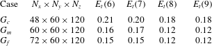
. Table 2 lists a representative set of FSDS3D simulations with different grid numbers
 $N_{x}\times N_{y}\times N_{z}$
and time step size of
 ${\rm\Delta}t=0.001L/V$
. In our simulations, we specify the initial 3D static displacement
 $z={\it\zeta}(x,y,0)$
as in (5.1) with
 $n=1$
and
 $\mathscr{A}_{1}=\mathscr{B}_{1}=0.1L$
.
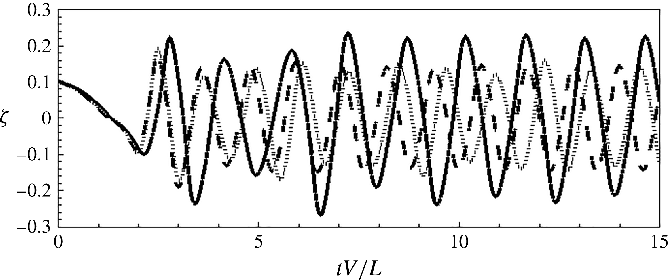
Time history of the cross-stream tail displacement
 ${\it\zeta}={\it\zeta}(x_{a},y,t)$
; for
 $G_{m}$
. Plotted for Reynolds number of (a)
 $\mathit{Re}=500$
(
 $\cdots \cdots$
), (b)
 $\mathit{Re}=800$
(– – –) and (c)
 $\mathit{Re}=1000$
(——).

Upon impulsive release, the system initially experiences a high-frequency oscillation of the spanwise displacement as it settles toward a flow-aligned configuration. Figure 25 plots the time history of
 ${\it\zeta}={\it\zeta}(x_{a},L,t)$
, with
 ${\it\mu}=0.125$
and
 ${\it\gamma}=5.0$
, for different
 $\mathit{Re}_{L}$
, which are all unstable to flapping. The
 ${\it\zeta}$
characteristics do not change significantly with increasing
 $\mathit{Re}_{L}$
, so we choose
 $\mathit{Re}_{L}=1000$
for our simulations. Table 2 clearly shows the conservation of the total energy (comprising the energy of fluid and flag)
 $E_{t}({\it\tau})=(E_{t}({\it\tau})-E_{t}({\it\tau}-1))(E_{t}({\it\tau}))^{-1}$
over five convective periods (
 ${\it\tau}=tV/L$
). For
 $C_{5}$
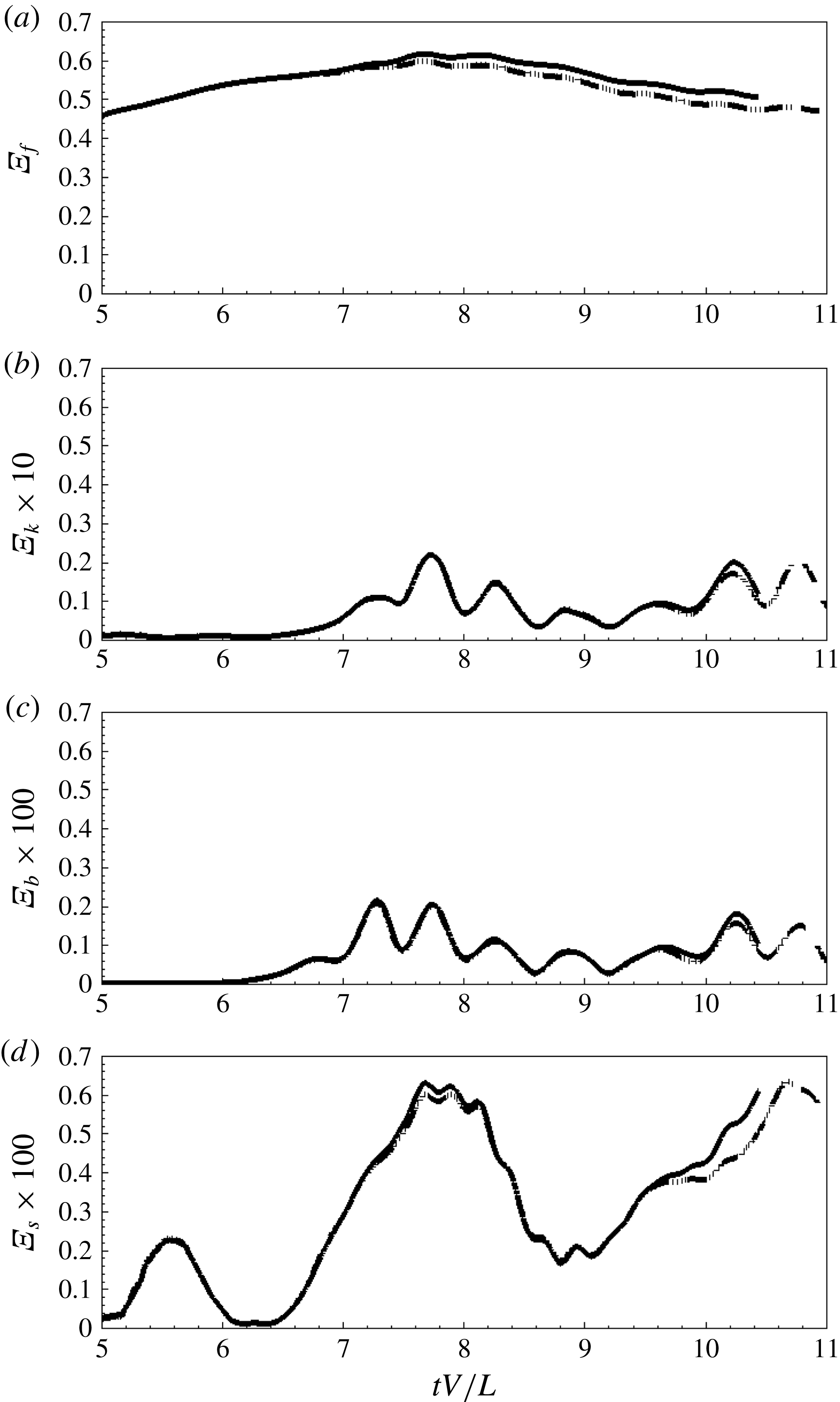
there is significant energy exchange between the fluid and structural domains. Figure 26 plots the evolution of the main components of
 $E_{t}$
, corresponding respectively to the fluid kinetic energy
 ${\it\Xi}_{f}$
, the structural kinetic energy
 ${\it\Xi}_{k}$
, the structural bending energy
 ${\it\Xi}_{b}$
, and the structural extensional energy
 ${\it\Xi}_{s}$
. Figure 26 shows the grid convergence for this problem for the different energy components spanning two orders of magnitude. Based on results such as this, we choose for all later results the
 $G_{m}$
:
 $N_{x}\times N_{y}\times N_{z}=60\times 60\times 120$
grid. Finally, comparing these energy amplitudes, it is clear that the near inextensibility and negligible bending rigidity assumptions hold.
Time history of (a) fluid kinetic energy
 ${\it\Xi}_{f}$
and (b) structural kinetic energy
 ${\it\Xi}_{k}$
(c) structural bending energy
 ${\it\Xi}_{b}$
and (d) structural extensional energy
 ${\it\Xi}_{s}$
. The lines correspond to
 $G_{c}$
(——),
 $G_{m}$
(– – –) and
 $G_{f}$
(
 $\cdots \cdots$
).

FSDS3D grid convergence for the total energy of the system
 ${\sim}$
(
 $-$
energy input
 $+$
fluid energy
 $+$
flag energy),
 ${\it\Xi}_{t}({\it\tau})$
using three different computational grids. The physical parameters used are:
 ${\it\gamma}=5.0$
,
 ${\it\mu}=0.125$
,
 $\mathit{Re}_{L}=1000$
,
 $K_{B}=0.0001$
, and
 ${\it\nu}_{s}=0.3$
.

Appendix B. Determination of the added mass
Following Lamb (Reference Lamb1932) and Yadykin, Tenetov & Levin (Reference Yadykin, Tenetov and Levin2003), the rate of change in time of kinetic energy of any portion of the fluid is equal to the work done by the pressures on the flag surface and is given as
 $$\begin{eqnarray}\frac{\text{d}E}{\text{d}t}=-\iint _{{\it\sigma}}V_{N}{\rm\Delta}p\,\text{d}{\it\sigma},\end{eqnarray}$$
where
 $E$
is the kinetic energy,
 ${\it\sigma}$
is the surface bounding the fluid region and
 $V_{N}$
denotes the velocity of a fluid particle in the direction of the normal
 $N$
. The last integral thus expresses the rate at which the pressure
 ${\rm\Delta}p$
, exerted from outside an element
 ${\it\delta}{\it\sigma}$
of the boundary, is doing work. Assuming the flag to be the fluid–solid interface, White (Reference White1991), (B 1) can be expressed as
 $$\begin{eqnarray}\frac{\text{d}E}{\text{d}t}=-\int _{0}^{S}\int _{0}^{L}\frac{{\it\delta}h}{{\it\delta}t}{\rm\Delta}p\,\text{d}s\,\text{d}x,\end{eqnarray}$$
where
 $\text{d}s=\sqrt{1+(\partial h/\partial x)^{2}}\,\text{d}y$
and
 ${\it\delta}h/{\it\delta}t$
is the velocity of the plate in the normal direction. For sufficiently small oscillations, the flag surface movement is more or less parallel to the
 $y{-}x$
plane, and
 ${\it\delta}h/{\it\delta}t$
approximates the normal velocity quite well. Following the work of Minami (Reference Minami1998), we derive the rate of change of kinetic energy in time of an oscillating flag having a mass per unit area equivalent to the added mass,
 $m_{a}$
, as
 $$\begin{eqnarray}\frac{\text{d}E}{\text{d}t}=m_{a}\int _{0}^{S}\int _{0}^{L}\frac{{\it\delta}^{2}h}{{\it\delta}t^{2}}\frac{{\it\delta}h}{{\it\delta}t}\,\text{d}s\,\text{d}x.\end{eqnarray}$$
Equating (B 2) and (B 3) the expression for
 $m_{a}$
can be derived in the form
 $$\begin{eqnarray}m_{a}=\left.-\int _{0}^{S}\int _{0}^{L}\frac{{\it\delta}h}{{\it\delta}t}{\rm\Delta}p\,\text{d}s\,\text{d}x\right/\!\int _{0}^{S}\int _{0}^{L}\frac{{\it\delta}^{2}h}{{\it\delta}t^{2}}\frac{{\it\delta}h}{{\it\delta}t}\,\text{d}s\,\text{d}x.\end{eqnarray}$$
The fluid loading on a unit area of an infinite flag surface, see Lamb (Reference Lamb1932), is given as
 $$\begin{eqnarray}{\rm\Delta}p=m_{a}\left(\frac{\partial }{\partial t}+V\frac{\partial }{\partial y}\right)^{2}z(y,t),\end{eqnarray}$$
where the fluid has a constant velocity
 $V$
parallel to the
 $y{-}x$
plane;
 $t$
is the time. Following Coene (Reference Coene1992), Connell & Yue (Reference Connell and Yue2007) derived
 $m_{a}^{2D}=2{\it\rho}_{f}L/k_{y}$
. Another estimate of the coefficient of the added mass per unit area,
 $m_{a}^{3D}$
, of a finite length flag can be made following the work of Wu (Reference Wu1961) and is given as
 $$\begin{eqnarray}m_{a}^{3D}=\frac{{\it\rho}_{f}L}{{\rm\pi}}{\it\gamma}\left(\frac{{\rm\pi}}{2}\right)^{2},\end{eqnarray}$$
where
 ${\it\gamma}$
is the aspect ratio of the plate. Table 3 lists the definitions of the added mass for 2D and 3D cases.
Determination of the added mass for various
 ${\it\gamma}$
.

Appendix C. Normal modes of a three-dimensional flag
We start with (2.1), and assume linearly varying streamwise tension and constant spanwise tension, no fluid loading and neglect moment due to shear stress. An estimate of the flow-induced tension force as compared to the magnitude of other forces is made using the physical parameters
 $K_{B}=0.0001$
,
 ${\it\nu}_{s}=0.3$
and
 $\mathit{Re}_{L}=1000$
. For a mode equal to the length of the membrane,
 $k_{y}=2{\rm\pi}$
, we find that the flow-induced tension force scales as
 $1.3\mathit{Re}_{L}^{-1/2}k_{y}^{2}$
, which is an order of magnitude higher than the bending force which scales as
 $K_{B}k_{y}^{4}$
. This predominance of flow-induced tension force persists at
 $\mathit{Re}_{L}=1000$
, for different
 ${\it\gamma}$
, making the assumptions for the derivation of the modes valid. We obtain
 $$\begin{eqnarray}\displaystyle \frac{\partial ^{2}{\it\zeta}}{\partial t^{2}}=c^{2}\left(\frac{\partial ^{2}{\it\zeta}}{\partial y^{2}}-\frac{1}{y}\frac{\partial {\it\zeta}}{\partial y}-\frac{1}{y^{2}}\frac{\partial ^{2}{\it\zeta}}{\partial x^{2}}\right), & & \displaystyle\end{eqnarray}$$
where
 $c^{2}=1.3\mathit{Re}_{L}^{-1/2}/{\it\mu}$
, and it is assumed that the spanwise tension is bounded by the maximum chordwise tension. The analysis of Moretti (Reference Moretti2003) considers in detail the sources and influence of tension in the body, citing the original work of Thoma (Reference Thoma1939) which highlights the importance of dynamically induced tension. They explain that during active flapping, the tension induced by the flapping motion becomes very significant, and Moretti (Reference Moretti2004) hypothesize that it is this dynamically induced tension which limits the flapping amplitude. Consistent with this, we assume inextensibility in the chordwise direction (only), and impose chordwise boundary conditions corresponding to clamped leading-edge and free (bounded) trailing-edge displacements:
 $$\begin{eqnarray}\displaystyle {\it\zeta}(x,0,t)=0,\quad \Vert {\it\zeta}(x,1,t)\Vert <\infty . & & \displaystyle\end{eqnarray}$$
Using separation of variables
 ${\it\zeta}=X(x)Y(y)\cos ({\it\omega}t-{\it\epsilon})$
, a series solution of the boundary value problem (C 1) and (C 2) can be expressed as
 $$\begin{eqnarray}\displaystyle \left(y^{2}\frac{\text{d}^{2}Y}{\text{d}y^{2}}-y\frac{\text{d}Y}{\text{d}y}+\frac{{\it\omega}^{2}}{c^{2}}y^{2}Y\right)=\frac{Y}{X}\frac{\text{d}^{2}X}{\text{d}x^{2}}\equiv n^{2}, & & \displaystyle\end{eqnarray}$$
where
 $n$
is a constant. Assuming spanwise wavenumber
 $k_{x}=2{\rm\pi}n/S$
,
 $n=0,1,2,\ldots ,$
we have
 $$\begin{eqnarray}\displaystyle X=\mathscr{C}\sin (nx-{\it\beta}),\quad Y=\mathscr{A}\text{J}_{n}\left(\frac{{\it\omega}(1-y)}{c}\right)+\mathscr{B}\text{Y}_{n}\left(\frac{{\it\omega}(1-y)}{c}\right), & & \displaystyle\end{eqnarray}$$
where
 $A$
,
 $B$
,
 $C$
are arbitrary constants and
 $\text{J}_{n}$
and
 $\text{Y}_{n}$
are Bessel functions of the first and second kind. From the second condition of (C 2b
), we have
 $\mathscr{B}=0$
. Finally, using the boundary condition
 ${\it\zeta}(x,1,t)=0$
, we obtain
 $$\begin{eqnarray}{\it\zeta}(x,y,t)=\text{J}_{n}({\it\alpha}_{n,m}(1-y))(\mathscr{A}_{n,m}\cos (n2{\rm\pi}/{\it\gamma}x)+\mathscr{B}_{n,m}\sin (n2{\rm\pi}/{\it\gamma}x))\cos (c{\it\alpha}_{n,m}t-{\it\epsilon}),\end{eqnarray}$$
where
 ${\it\alpha}_{n,m}$
denotes the
 $m$
th (positive) root of
 $\text{J}_{n}$
. These normal modes can be used as initial conditions for simulations. Conversely, an arbitrary initial displacement can be decomposed in terms of the normal modes (C 5).