

1. Introduction
Services have become increasingly tradable in recent decades, as sectors, such as business services, no longer require face-to-face proximity for transactions to be carried out. However, despite this recent shift, there remain some service sectors where face-to-face interactions between producers and consumers are necessary. The share of services in international trade volumes has risen, with services now accounting for 20% of global trade. The main drivers of this increase have been technological improvements in the information and communication areas (Bensidoun and Ünal-Kesenci, Reference Bensidoun and Ünal-Kesenci2008). Trends also indicate that this share should rise in the coming decades.
Services cannot be treated in the same way one treats goods. Initially, the main differences between them were identified as lying in services' lack of storability and the need for interactions between the user and the producer (Bhagwati, Reference Bhagwati1984, Reference Bhagwati1985; Sampson and Snape, Reference Sampson and Snape1985). It is important, however, to take into account the diversity among services. For instance, financial and health services differ completely in their nature, in their mode of supply, and in their need for proximity between producer and consumer. Obviously, if trade in goods and trade in services must be differentiated, service barriers will also differ from the goods barriers, not least through the latter's greater reliance on non-tariff barriers such as obligations for joint-ventures to establish a commercial presence, the need for operating licenses, the limited number of visas for key workers, etc. Such barriers are clearly likely to influence firms' trading choices. For example, prohibitive fixed costs of establishment may force foreign suppliers to serve a market through cross-border supply instead of a commercial presence abroad, which may negatively impact the quality and the varieties of services on the market, and may generate welfare losses. In impeding market access to foreign suppliers, barriers to services reduce the efficiency of the services market often by curtailing competition. Markusen and Strand (Reference Markusen and Strand2008) show that liberalizing services leads to large welfare gains due to a more competitive services market, leading to more efficient manufacturing productions in their model, as services are considered as inputs.
The General Agreement on Trade in Services (GATS) was created in 1995 to lead the further multilateral liberalization of services trade, including in negotiations. The first article of the text defines the field by designating services as follows: ‘“services” includes any service in any sector except services supplied in the exercise of governmental authority’. Liberalization in services would generate gains of approximately $130 billion including the larger gains for China (Dee and Hanslow, Reference Dee and Hanslow2000).
The aim of the present paper is to estimate the current degree of restriction in services trade, and to assess the restrictive impacts of regulations on trade in services by sector.
For trade in goods, the importance of distinguishing between products has been clearly shown. The determinants of trade can significantly differ across sectors, and according to Rauch (Reference Rauch1999), Linders (Reference Linders2004), and Möhlmann et al. (Reference Möhlmann, Ederveen, Groot and Linders2009) this product heterogeneity must be considered when assessing the impacts of barriers; it gives rise to sectoral analyses. Along the same lines, services, as well as barriers related to trade in services, are heterogeneous. We therefore conduct a sectoral analysis, which allows consideration of the specificities present in different services. We deal with non-tariff barriers by using a gravity-based approach to calculate tariff equivalents. This method is convenient as it avoids having to weight together different barriers to get an overall total. Because the standard gravity equation is estimated in logs, however, it is necessary to deal with zero flows in the database, especially because at a sectoral level zero flows are more common than in aggregates. Indeed, in our data, zero flows represent approximately 66% of the flows for personal, cultural, and recreational services, and, on average, they account for approximately 45% of flows. Not taking into consideration this important feature would bias the results of the estimation, and thus the estimated tariff equivalents. I opt for the Heckman selection model to handle this issue. The derivations of the tariff equivalents are based on the distribution of the residuals from a gravity model. The barriers identified from trade data, as ours are, relate strictly only to mode 1 (i.e., cross-border supply) but within this category they include both pure cross-border trade (unaffiliated sales) and related-party trade between affiliates.Footnote 1
The structure of the paper is as follows. In the next section, I provide an overview of the different methods used to measure tariff equivalents, followed by a description of my own methodological approach. After presenting the data, the results are documented in Section 5 and conclusions are discussed in Section 6.
2. Review of the literature
Deardoff and Stern (Reference Deardorff and Stern1998) classify the methods used to quantify trade barriers into three categories: frequency and coverage indices, sometimes called the qualitative method, quantity-based measures which rely on gravity models, and price-based measures.
Considering the General Agreement on Trade in Services commitments of each country, Hoekman (Reference Hoekman1995) creates a frequency index of restrictiveness based on the assignment of a numerical value according to the level of restriction. The Hoekman index reflects a strong link between the level of GDP per capita and the number of GATS commitments. Arbitrary weightings are assumed to generate these indices, with both minor and major obstacles having the same weight, which clearly reduces their accuracy as measures of the degree of protection offered. The Hoekman indices are relative indicators, not real indices, and cannot be used as tariff equivalents (Stern, Reference Stern2000). The Australian Productivity Commission (APC) considers several sources to list trade barriers. This permits one to estimate tariff equivalents more accurately. However, each of the APC studies focuses on a single sector: distribution in Kalijaran (Reference Kalirajan2000), maritime transport in McGuire and Schuele (Reference McGuire, Schuele, Findlay and Warren2000), telecommunications in Warren (Reference Warren, Findlay and Warren2000); or on two sectors (telecommunications and financial services) as in Mattoo et al. (Reference Mattoo, Rathindran and Subramanian2006).
Price-based measures depend on differences between domestic and foreign prices to assess the barriers to entry on the national market (Deardoff and Stern, Reference Deardorff and Stern1998). Francois and Hoekman (Reference Francois and Hoekman1999) base their approach on gross operating margins. The margins are a gauge of the relative profitability of the different industries and arguably capture barriers to foreign competition. The APC provides several works deriving from these price-based measures, such as Nguyen-Hong (Reference Nguyen-Hong2000) for engineering services, Trewin (Reference Trewin, Findlay and Warren2001) for telecommunications, or Kalirajan et al. (Reference Kalirajan, McGuire, Nguyen-Hong, Shuele, Findlay and Warren2001) for banking. In addition, relying on a weighting methodology, Dihel and Sheperd (Reference Dihel and Sheperd2007) compute sectoral, aggregate, and then modal trade restrictiveness indices from price-cost margins. A two-stage method is required to estimate the impacts of the existing barriers, given by the price-cost margins. First, the price-cost margins are determined at the firm-level, and then the effects of the trade restrictions on price-cost margins are analyzed at the sectoral level. They apply their methodology to banking and insurance, telecommunications, professional services, and to distribution.
Gravity models have been applied to trade in services. Francois (Reference Francois2001) shows that the standard set of controls used in the gravity equation is significant also for services. To explain bilateral trade in services, Kimura and Lee (Reference Kimura and Lee2006) include country-specific determinants, such as GDPs, remoteness (how far a country is relative to the rest of the world), economic freedom, and country-pair-specific determinants, such as sharing a common language, a common border, and a common trade agreement. All these variables are significant. Moreover, they find that the power of explanation of gravity models is significantly larger for trade in services than for trade in goods.
Francois (Reference Francois2001) is one of the first studies to estimate tariff equivalents from quantity-based measures. The first step consists of estimating a gravity equation using OLS. From these estimates, the bilateral trade flow for each country-pair is predicted. From the comparison between the actual and the predicted trade, the tariff equivalents for the services barriers are derived assuming a constant elasticity import demand function. Francois et al. (Reference Francois, van Meijl and van Tongeren2003) estimate sector-specific gravity equations to obtain services barriers using Global Trade Analysis Project (Gtap) data. Imports in a given sector are explained by the GDP per capita, the population in the importing country, and a dummy for European countries. Using an elasticity of substitution of 4.67, India is the most protected country in the world, while Sub-Saharan Africa and the Netherlands have 0% trade cost equivalents for the four services sectors he considers.
Park (Reference Park2002) follows the Francois (Reference Francois2001) method to calculate the tariff equivalents. He bases his gravity equation on Deardoff (Reference Deardorff1998) and, at least partially, on Anderson and van Wincoop (2003) because the prices are tackled differently. Park (Reference Park2002) uses Gtap data and includes producer price indexes to account for prices. Bilateral trade in services is explained by the GDP of countries, distance, the aggregate wholesale price indices in importing and exporting countries, and a set of dummies (common language, regions). Park derives tariff barriers for seven different services sectors and 62 countries. The level of openness is not homogeneous for every sector of a country, and the level of development is not systematically correlated with a high level of protection. Park (Reference Park2002) finds that, on average, Asian countries are less protected than other countries in the sample.
Walsh (Reference Walsh2008) estimates a specific gravity equation for four sectors (transport, government, other commercial services, and travel). The explanatory variables are close to those used in the previous studies: GDP per capita, population, distance, adjacency, common language, and a dummy for the European Union membership. However, Walsh (Reference Walsh2008) adds sector-specific variables, including government efficiency for the government sector, temperatures for travel, and economic freedom for commercial services. To address biased estimates using OLS, Walsh (Reference Walsh2008) applies the Hausman and Taylor model to services trade. Again, the tariff equivalents come from the difference between actual and predicted trade. Using a similar method as Park (Reference Park2002), but with an elasticity of substitution of 1.95, Walsh (Reference Walsh2008) finds average tariff equivalents ranging from 0% (for Japan, Norway, and Belgium) to 125% (for Indonesia).
In this analysis, I rely on the gravity equation methodology. Taking residuals from gravity equations represents a convenient base to calculate tariff equivalents. An advantage of this method is that it relies on a limited series of easily available data, which allows for its application to a large set of countries without relying on specific data collection. The negatives in using the method range from the sensitivity of the results obtained to the specification of the gravity equation estimated, to the quality of the data and to the sample of countries. In addition, tariff equivalents do not permit one to quantify the effects due to a given policy, but rather provide a global overview of the level of openness in services with all barriers taken together. The information contained in the tariff equivalents by sector is complementary to other services regulation indices such as product market regulation (PMR) indices provided by OECD or the index of bilateral regulatory heterogeneity based on policy items and developed by Kox et al. (Reference Kox, Lejour and Montizaan2004).Footnote 2
Compared with previous studies, attention here is particularly focused on the zero flows issue in the econometric methodology and in the calculation of tariff equivalents. Indeed, when countries do not trade and one could expect them to trade according to their characteristics, we are faced with a sample selection problem. In this context, using sample OLS estimations would lead to biased results, as the observed sample is not representative.
3. Methodology
3.1 The specification of the gravity equation
The gravity equation was introduced into international trade research in Tinbergen (1962) where the international bilateral trade was found to be positively related to the level of the GDP of both countries and negatively related to the distance. The theoretical foundations of the gravity equation have been developed over time. Anderson (Reference Anderson1979) was the first to elaborate a theory using the Armington assumption. Bergstrand (Reference Bergstrand1985) derived price indices in a monopolistic competition framework. Anderson and van Wincoop (Reference Anderson and van Wincoop2003) include multilateral resistance terms (MRTs) to emphasize the idea that bilateral trade depends on the relative trade costs between the two trading partners. Empirically, the MRTs can be estimated using country fixed effects for both the importer and the exporter. Helpman et al. (Reference Helpman, Melitz and Rubinstein2008) develop a model of trade with heterogeneous firms explaining zero flows, asymmetric trade flows, and extensive margins.
Taking into account all the possible theoretical findings, the following gravity equation is estimated. Note that the set of controls used is standard and close to the explanatory variables used by Park (Reference Park2002). In the robustness analysis, other specifications are tested.
 $$\eqalign{\ln X_{ijs} = &\ \alpha _1 + \alpha _2 \ln (GDPpc_i ) + \alpha _{3{\rm}} \ln (GDPpc_j ) + \alpha _4 \ln (Pop_i ) + + \alpha _5 \ln (Pop_j ) \cr & + \alpha _{6{\rm}} \ln (Dist_{ij} ) + \alpha _7 Comlang_{ij} + \alpha _8 Colony_{ij} + \alpha _9 Contig_{ij} \cr & + \alpha _{10} Island_{ij} + \alpha _{11} Landl_{ij} + \alpha _{12} RTA_{ij} + \varepsilon _1} $$
Trade from country i to country j in sector s depends on the GDP per capita, the population of each country, and the distance between them. Some dummies are added such as common language (represented by Comlang ij), common past (Colony ij), common border (Contig ij), a variable to account for membership in the same regional trade agreement (RTA ij), and dummies if either country i or j is an island (Island ij) or is landlocked (Landl ij).
This analysis is based on cross-sectional data using predictions to calculate tariff equivalents. If we included country fixed effects, all the country characteristics of importer and exporter would be captured by the dummies. The R-squared would increase substantially, but the importer-country-specific effect of commercial policy would be absorbed into the importer fixed effect. This would bias the tariff assessments downwards by reducing the residuals to the extent that all of an importer's partners faced the same barriers. Therefore, the methodology recommended by Helpman et al. (Reference Helpman, Melitz and Rubinstein2008) − that is to say that a Heckman sample selection model using a probit and non-linear least squares with controls based on fixed effects coefficients − is not feasible here. The Anderson and van Wincoop (Reference Anderson and van Wincoop2003) recommendation is also not appropriate in this case.
3.2 Zero flows
Until recently, estimating gravity equations did not take into account zero flows. However, this issue has increasingly been considered (see Bikker and de Vos, Reference Bikker and De Vos1992 ; Soloaga and Winters, Reference Soloaga and Winters2001; Rose, Reference Rose2004; Linders and de Groot, Reference Linders and De Groot2006; Helpman et al., Reference Helpman, Melitz and Rubinstein2008). Frankel (Reference Frankel1997) highlights the presence of the zero flows, particularly for small and remote countries. It is noteworthy that 27% of the bilateral trade matrix is empty in Haveman and Hummels (Reference Haveman and Hummels2004).
In the sample considered here, I have to take into consideration zero flows. Indeed, zero flows represent between 12% (transport) and 66% (personal, cultural, and recreational services) of flows depending on the sector. This is a common phenomenon, particularly when a large number of countries is considered or when there is sectoral disaggregation. It is not surprising that Brazil and Croatia do not trade financial services in a given year, for instance.
Among zero flows, there are both missing values and genuinely null trading flows. The latter contain meaningful information. Indeed, it might be interesting to know more about why countries trade in some sectors and why the same country pair does not trade in others. In the database I used, it is possible to differentiate null flows from missing values, because two cases occur: (1) ‘.’ is considered as a missing value and (2) ‘0’ is treated as a null flow in the analysis. I verify the consistency of zero flows by comparing it with the trade of the previous years. Note that the unit is in millions; consequently, if the countries trade less than one million, the bilateral trade will be recorded as zero.Footnote 3
To use the gravity equation in the log-linear form, this problem must be addressed. In dropping zero flows, potential information is removed and it biases the estimated coefficients. Recent literature has acknowledged three main methods to address the issue.Footnote 4
The first method, which is not theoretically founded, consists of an ad hoc solution whereby the ‘0’ is replaced by a very small value for which the log is defined. In the same way, the censored regression model (tobit) accounts for zero flows.Footnote 5 A lower limit is defined, and all the values below this threshold are censored. Because the residuals of censored observations tend to be positive and not necessarily low, Martin and Pham (Reference Martin and Pham2008) underline the inefficiency of this method, as the coefficients of the control variables are biased downward. Furthermore, Linders and de Groot (Reference Linders and De Groot2006) show that the choice of the threshold is important.
The Poisson model is also an option (Santos Silva and Tenreyro, Reference Santos Silva and Tenreyro2003 and Reference Santos Silva and Tenreyro2006). In this methodology, the dependent variable is in levels while the explanatory variables are in logs. Thus, zeros are included in the estimation of a gravity model. All observations are weighted equally. To some extent, no special attention is given to zero flows, assuming that the absence of trade between two countries is not particular. Nevertheless, equal weights can be inappropriate if the reliability of reporting trade flows is not uniform in the sample considered. Indeed, a large reported volume of trade may be more reliable than a small trade volume. Thus, weighting these trade flows equally can be inconsistent.
Because the trading probability can be correlated with some control variables included in the gravity equation, excluding the probability of positive trade flows biases the results. This leads to two distinct questions: ‘Do the countries trade?’ If they do: ‘How intense is the potential bilateral flow?’ Since countries select their trading partners, the Heckman two-stage selection model proposes a convenient and appropriate alternative to account for the zero flows and to deal with these two questions. Martin and Pham (Reference Martin and Pham2008) estimate the gravity equation using several techniques to overcome the large share of zero flows. They find that the Heckman sample selection estimator provides good results to determine bilateral trade in the case of zero flows when a selection variable is included. Linders and de Groot (Reference Linders and De Groot2006) find similar results. One practical disadvantage of this method is the requirement for an excluded variable, which explains the propensity to trade but not the amount.
3.3 Sample selection model
In the Heckman selection model (Heckman, Reference Heckman1979), there are two steps: two latent sub-models using maximum likelihood methodologies. The first stage, using a probit model, estimates the probability that trade occurs between the two countries and that the observation is different from zero in the sample. The second stage corresponds to a least squares estimation of the existing trade with a gravity equation, including the probability to trade based on the probit estimation. It is expected that the explanatory variables play a different role in explaining the existence of a commercial relationship and explaining the volume of trade. The Heckman sample selection is the OLS regression augmented by an otherwise omitted regressor that reflects selection (the inverse Mills ratio). When the inverse Mills ratio is significant, this means that the correction for sample selection in the second stage is needed and that omitting it will lead to bias. Cameron and Trivedi (Reference Cameron and Trivedi2005) demonstrate the efficiency of Heckman sample selection estimator.Footnote 6
The decisions of the firms based on the evaluation of the fixed costs of market entry seem to fit a two-stage procedure. The presence of sunk costs generates potential zero flows. Indeed, Bernard and Jensen (Reference Bernard and Jensen2004) show that the fixed costs represent a significant part of the decision to export, which is viewed as a standard profit-maximizing decision (see also Anderson and van Wincoop, Reference Anderson and van Wincoop2004). In the same way, in Helpman et al. (Reference Helpman, Melitz and Rubinstein2008), zero flows correspond to a situation in which no firm is productive enough in a country to export to another country.
Felbermayr and Kohler (Reference Felbermayr and Kohler2006) promote a combined gravity model to analyze both, arguing that there is no reason why the trading relationship and the volume of trade, if this relationship exists, should be explained by different determinants. Francois and Manchim (Reference Francois and Manchin2007) jointly estimate the probability of trade and the amount of trade. Similarly, I assume that the decision to trade and the decision regarding the volume of trade can be explained by the same variables except for the variable denoting the sharing of a common religion, which I use as a control contained only in the first step.
The empirical strategy can be summed up as follows:
Equation (1) is observed if and only if
 $$\eqalign{\theta _1 + & \theta _2 \ln (GDPpc_i ) + \theta _3 \ln (GDPpc_j ) + \theta _4 \ln (Pop_i ) + \theta _5 \ln (Pop_j ){\rm} \cr & + \theta _6 \ln (Dist_{ij} ) + \theta _7 Comlang_{ij{\rm}} + \theta _8 Colony_{ij} + \theta _9 Contig_{ij} \cr & + \theta _{10} Island_{ij} + \theta _{11} Landl_{ij{\rm}} + \theta _{12} RTA_{ij} + \theta _{13} Exclusion_{ij} + \varepsilon _2 \gt {\rm} 0} $$
The selection equation must contain at least one exclusion variable which is not contained in the gravity equation. In the literature, there is no consensus on an instrumental variable affecting the trading probability but not affecting the level of trade. Helpman et al. (Reference Helpman, Melitz and Rubinstein2008) propose religious ties (interactions between the shares of Protestants, Muslims, and Catholics for the two countries) and regulation costs as instruments. Although some empirical analyses show that sharing similar beliefs has no impact or only a weak impact on international trade (Lewer and Van den Berg, Reference Lewer and Van den Berg2007), there is some evidence of links between trade and measures of religiosity when the view of different cults on trade is taken into account (Helble, Reference Helble2007), through the increase of economic performance (Barro and McCleary, Reference Barro and McCleary2003), or specifically through intra-regional trade (Guo, Reference Guo2007). Guiso et al. (Reference Guiso, Sapienza and Zingales2003) and Guiso et al. (Reference Guiso, Sapienza and Zingales2006) highlight the cultural-based effect on economic growth due to economic behaviors conducive to economic activity (attitudes towards cooperation, respect of legal rules, etc.), and cults can determine economic attitudes to some extent (see Iannoccone, Reference Iannaccone1998; Dark, Reference Dark2000; Welch and Mueller, Reference Welch and Mueller2001, for the linkage between religion and economics). Thus, countries sharing cultural proximity, affinities, and common beliefs are more likely to trade than countries that have dissimilar cultural and religious values. Unlike Helpman et al. (Reference Helpman, Melitz and Rubinstein2008), I allow for more than three cults: Anglicanism, Buddhism, Catholic Church, Evangelicalism, Hinduism, Judaism, Islam, Orthodoxy, Protestantism, Shinto, and Taoism. I generate a dummy variable equal to 1 if the two countries have a common main religion.
3.4 Tariff equivalents
Based on the previous estimation, bilateral trade is predicted for every service sector. I then compute the residuals for each importer and each sector. A crucial assumption is then made: the free-trade country, which I use as the benchmark for a given sector, is defined by the largest positive difference between the predicted and real trade. The difference between a country's residual and this benchmark value corresponds to the level of trade barriers. Although the residuals contain a variety of information, including on commercial policy, the predicted–actual trade ratio has been interpreted as the potential–actual trade ratio by Baldwin (Reference Baldwin1994), Nilsson (Reference Nilsson2000), and Egger (Reference Egger2002). Trade inefficiencies impede bilateral trade and cause actual trade to fall below potential trade. Because the estimated trade potential of a given country refers to the hypothetical situation with fewer barriers, it is defined by the frontier. The benchmark is used to estimate trade resistances and compare trade performances across countries. Obviously, the reliability of the estimation of the tariff equivalents is completely dependent on the quality of predictions, and therefore on the quality of specification of the gravity equation and in particular on the residual that emerges for the benchmark country.
Park (Reference Park2002) and Walsh (Reference Walsh2008) obtain the tariff equivalents from the ratio between predicted and real trade.
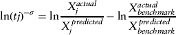 $$ {\ln (tj)^{ - \sigma}} = \ln\displaystyle{{X_j^{actual}} \over {X_j^{^\displaystyle{\,predicted}}}} - \ln\displaystyle{{X_{benchmark}^{actual}} \over {X_{benchmark}^{\,predicted}}} $$
where X j represents the sum of trade over all trading partners of country j. Xactual and Xpredicted are, respectively, the total of the actual and predicted imports of all the partners.Footnote 7
Because the question of interest is how easy it is to have access to a given market for foreign products/services, only imports are logically considered in the assessment of non-tariff barriers, and the level of imports is important to determine the openness of a country. Thus, the question regarding the ease of exporting home products/services (including possible subsidies) is not considered in these analyses. Nevertheless, a reason why foreign suppliers can have difficulty selling in a given market is comparative advantage such that home demand is largely satisfied by national providers at more competitive prices than non-national providers. In this case, a lack of imports does not mean that this country is protected. In considering only imports, the law of comparative advantage is ignored, thus leading to tariff equivalents that do not account for country characteristics and specializations on the production side. According to this formula, if a country has a comparative advantage in a given sector, it will be considered as a non-open country with a high tariff equivalent insofar as the imports are lower than the predicted imports. This does not mean that this country does not participate in international trade. In the presence of a comparative advantage, a country has higher exports than those predicted in a sector.
Consequently, to address this issue, X j in equation (3) represents the total of imports plus exports. Thus, the tariff equivalents obtained reflect policy-imposed measures to discourage foreign providers, natural barriers to trade, and comparative advantage.
Because an overestimated difference between actual and predicted trade leads to a misrepresentation of the degree of openness for these countries, the quality of predictions is crucial. The dependent variable is in logs. However, taking the natural logarithm of the predicted bilateral trade is wrong because the variable of interest is the level of trade and also because exp{E(lnXij)}≠ E(Xij). The back-transformation for the lognormal distribution that I use takes into consideration the correction proposed by Aitchison and Brown (Reference Aitchison and sBrown1957). Assuming the following log-linear model ln(X)=a + b ln(Y) + u, and u ∼ N(0;σ 2), the prediction of X is obtained from the OLS estimates of the parameters a, b, and σ 2:  $X^{\,predicted} = \exp (\hat a + \hat b\,\ln (Y) + \hat{\sigma} ^{2} /2$). In the case of Heckman sample selection, the post-estimation predicted trade uses the inverse of the Mills' ratio, noted λ(y 1′ β 1). According to Cameron and Trivedi (Reference Cameron and Trivedi2005), the predicted trade of importing countries with a positive actual trade is based on the following expression taking into consideration the retransformation issue
 $$E(X_2 |y,X_1 \gt 0) = y_2 \prime \beta _2 + \sigma _{12} \lambda (y_1 \prime \,\beta _1 )$$
where X 1 and X 2 determine respectively whether two countries trade, and the level of trade that is observed if X 1 > 0; y 1 and y 2 are the vectors of regressors of each step. By assumption, the errors are jointly normally distributed and homoskedastic; σ 12 is the covariance parameter.
In Equation (3), total actual and predicted trade of country j across its partners are obtained respectively from the sums of actual and predicted bilateral flows for a given country j. The benchmark country is the country for which the difference between actual and predicted trade is the largest. The tariff equivalent is obtained from the comparison between this ratio for the country itself and that for the benchmark country.
From Equation (3), I obtain the tariff equivalent for the importer, country j
 $$tariff_{j} = t_{j}-1$$
Another essential assumption concerns the elasticity of substitution. The values of tariff equivalents are sensitive to the specification, to the sample considered and to the elasticity of substitution. In the literature, there is no accurate measure for the elasticity of substitution, σ, between services supplied by different countries. Consequently, I follow the previous papers on this topic. Tariff equivalents have been calculated with values of 5.6 as in Park (Reference Park2002) and 1.95 as in Walsh (Reference Walsh2008). Because σ is involved only in the final calculation of the tariff equivalents, not in the estimation of the residuals, the value chosen has a major influence on the magnitude of tariff equivalents but not on the ranking of countries nor the extent to which their trade is estimated to fall short of potential. Consequently, only the results with an elasticity of substitution at 5.6, as in Park (Reference Park2002), are presented here.
4. Data
This analysis is based on cross-border trade in services. Hoekman (Reference Hoekman1995) notes the weaknesses of data on trade in services. Although the GATS has encouraged countries to report data since the 1990s, measuring international trade in services is not a straight-forward statistical task (see Cave, Reference Cave2006; Giovannini and Cave, Reference Giovannini and Cave2007; and Bensidoun and Ünal-Kesenci, Reference Bensidoun and Ünal-Kesenci2008). However, the Manual on Statistics of International Trade in Services (EC et al., 2002), clarifies the nomenclature and correspondence between statistical systems. Lipsey (Reference Lipsey2009) highlights the increasing number of countries reporting exports and imports of services by sector over time. For example, the number of countries reporting exports of communication services doubled between 1993 and 2003. Similarly, Lejour et al. (Reference Lejour, Van Leeuween and ten Gate2008) test the reliability of data on trade in services for the OECD source for the year 2004. They find that the reliability is not homogeneous across sectors and across countries, e.g., data are more available in the travel sector than in the insurance sector. However, as they note, the reliability increases over the years. The Gtap database has been used to calculate tariff equivalents (see Section 2). Gtap version 7.4 provides bilateral flows for 80 countries for a large number of sectors. However, a gravity model has been already used to balance the latest versions of the matrices, so this source is not suitable for our use.
Eurostat statistics provide tables on international trade in services. A very advanced disaggregation is proposed for 2005. In taking the most detailed services flows, more missing values occur. Therefore, to keep the sectoral dimension in the analysis, I utilize the Eurostat ITS database on services with the level of disaggregation used in Brandicourt et al. (Reference Brandicourt, Schwellnus and Wörz2008). This covers the export flows for the year 2005 for 63 countries. The ITS database is complemented with the OECD database for Australia, New Zealand, and Canada. In this paper, the sectors considered are transportation, other business services, travel, communication services, construction, insurance, financial services, royalties and license fees, computer and information services, personal, cultural and recreational services, and government services. Even if the GATS negotiations do not include government services trade, some does exist. This sector is composed of transactions by embassies, consulates, military units, and defense agencies with residents of a country where they are located.
In addition, the CEPII distances database gives the bilateral geographic distance between trading partners (between capital cities in kilometers). It also includes some country-pair features, such as contiguity, common colony, and a common language variable (official language). I also use country-specific variables, such as landlocked. Concerning the GDP per capita and population data, I use the IMF statistics for the period considered. Moreover, a regional variable has been generated: it is equal to 1 if both countries belong to the same regional trade agreement such as the case of the European Union, Mercosur, Asean, Anzcerta, and Nafta. Concerning the religion variable, I use data provided by the CIA World Factbook and consider most of the religions for which I have information. If the most popular cult is the same in both countries, the dummy is equal to 1; otherwise, it is equal to 0.
5. Results
5.1 Estimation results
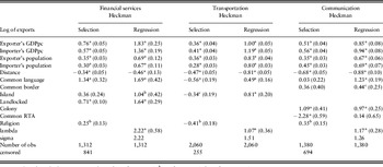
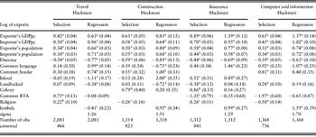
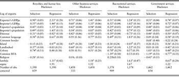
As noted, I estimate the gravity equation sector by sector in using the Heckman selection estimator. The standard control variables used in gravity estimations, such as GDP per capita, distance, language, etc. are significant and have the expected signs.Footnote 8 According to Table 1, distance is significant and negative for every sector, with a more or less important coefficient (lower for finance than for transport). Concerning the decision to trade, the standard determinants generally perform well and in some cases, the variables explain the decision to trade than they do the size of bilateral trade. Nevertheless, the determinants vary in nature and magnitude across sectors in both stages. GDP per capita and population explain both the choice of commercial partners and the trading volume. However, distance matters less for the selection than for the level of trade. For instance, in construction exports, the coefficient of distance is −0.59 for the first step, while it rises absolutely to −0.89 in the second step. In the same way, in Table 1 one can see that sharing a common language has no impact on the decision to trade for communication, insurance, other business services and travel, but significantly affects the amount of trade between partners. Membership of a common RTA impacts significantly trade in services for only one sector. This may be explained by the lack of negotiations on services even within the RTA. Contiguity impacts the trade between two bordering countries in three sectors − communication, travel, and construction − sectors which possibly require a degree of proximity to provide services. Note that contiguity is a significant determinant of the choice of the commercial partner and of the trading amount only for construction. Moreover, while a common past is important for trade only in communication and in government services, it is important for the decision to trade for seven of the 11 sectors. Only communication and government services consider the historic relationship when determining the existence of a commercial relationship and the trading level. Island and landlocked features do not seem to be obstacles to trade in the case of services. The positive sign of the island coefficient in construction is arguably explained by the need to build more in the case of small countries (in terms of area) such as Japan compared with large countries.Footnote 9 In addition, it is important to note that in the sample, countries with the island characteristic include among others Japan, Ireland, United Kingdom. Thus, it is not surprising that the coefficient is positive for some sectors, reflecting the tendency of these economies toward services exports.Footnote 10
Estimation results: financial services/communication/transportation

Notes: Value of standard-errors in parentheses; aSignificant at 1%; bSignificant at 5%; cSignificant at 10%.
The selectivity term, λ, is positive and significant for all sectors except for travel, highlighting the positive link between the two steps of the selection model.Footnote 11
(continued): Estimation results: travel/construction/insurance/computer and information services

Notes: Value of standard-errors in parentheses; aSignificant at 1%; bSignificant at 5%; cSignificant at 10%.
(continued). Estimation results: royalties and license feesl/other business services/personal, cultural and recreational services/government services

Notes: Value of standard–errors in parentheses; aSignificant at 1%; bSignificant at 5%; cSignificant at 10%.
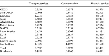
Table 2 displays the mean ratio of actual to predicted trade for different regions using the predictions of the Heckman sample selection. In most of the cases, predicted trade is greater than actual trade. For the three sectors considered in the table, the differences between actual and predicted trade range from 0.11 to 3.18, indicating the heterogeneity of trade barriers across countries and regions.
Mean ratio of actual to potential trade

Note: The predicted trade is based on Heckman sample selection estimates. The benchmark countries are: Hong Kong (transportation); Philippines (communication) and Luxembourg (financial services).
5.2 The level of trade barriers
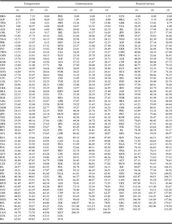
Table 3 and 4 display the estimates of the average tariff equivalents. Table 3 gives the tariff equivalents by country for transportation, communication, and financial services under different estimating methods. Columns (1) and (2) give the tariff equivalents based on Heckman estimations considering first the sum of exports and imports (1) and then imports only (2). Column (3), which I will discuss below, displays tariff equivalents based on the sum of exports and imports using OLS estimation.
Tariff equivalents in% for transportation/communication/financial services

Notes: (1) based on sum of imports and exports using Heckman sample selection postestimations; (2) basedon sum of imports using Heckman sample selection postestimations; (3) based on OLS estimates and on sum of imports and export. The tariff equivalents for the importer with the sum of imports and exports equals to 0 are not available. The sample is composed of: Albania (ALB); Argentina (ARG); Australia (AUS); Austria (AUT); Belarus (BLR); Belgium (BEL); Brazil (BRA); Bulgaria (BGR); Canada (CAN); Chile (CHL); China (CHN); Colombia (COL); Croatia (HRV); Cyprus (CYP); Czech Republic (CZE); Germany (DEU); Denmark (DNK); Egypt (EGY); Estonia (EST); Finland (FIN); France (FRA); Greece (GRC); Hong Kong (HKG); Hungary (HUN); Iceland (ISL); Indonesia (IDN); India (IND); Iran (IRN); Ireland (IRL); Israel (ISR); Italy (ITA); Japan (JPN); Latvia (LVA); Lithuania (LTU); Luxembourg (LUX); Malta (MLT); Malaysia (MYS); Mexico (MEX); Morocco (MAR); Netherlands (NLD); New Zealand (NZL); Nigeria (NGA); Norway (NOR); Philippines (PHL); Poland (POL); Portugal (PRT); Russia (RUS); Singapore (SGP); Slovak Republic (SVK); Slovenia (SVN); South Africa (ZAF); South Korea (KOR); Spain (ESP); Sweden (SWE); Switzerland (CHE); Thailand (THA); Taiwan (TWN); Turkey (TUR); Ukraine (UKR); United Kingdom (GBR); United States (USA); Uruguay (URY); Venezuela (VEN).
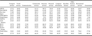
Average tariffs equivalents in% by regions

The ranking in column (2) diverges significantly from that in column (1), indicating the importance of considering both exports and imports as the base for estimating trade barriers. Indeed, in column (2) service exporters appear as protected countries, while the countries that are less involved in international trade in services, such as Uruguay in transportation, come at the top of the ranking.
Although the more open countries appear to be the developed ones, with the exception of the travel, construction, and recreational sectors, tariff equivalents of some developing countries, such as Indonesia or Turkey, are below the average tariff equivalents. Nevertheless, one of the limits of this methodology is that it tends to emphasize the positive difference between actual and predicted trade of countries not likely to trade due to their country characteristics compared with countries whose characteristics would suggest a strong likelihood of trading. By taking into account zero flows in the estimation and in the calculations of tariff equivalents, I have attempted to narrow down this difference.
Table 4 shows that the average of the tariff equivalents is approximately 50%, but it highlights considerable differences in trade barriers across sectors. Note, however, that these differences in average protection between sectors are strongly dependent on the size of the residual for the benchmark (least protected) country and so they need to be treated with some caution. The least protected sector is transportation services (at approximately 28%, on average) and the more protected sectors are financial and recreational services. Higher tariff equivalents in financial services may be explained by more reservations and exceptions in financial services in both multilateral and bilateral trade negotiations; according to the GATS coverage by country provided by the WTO, exemptions for the financial sector are important. They may also reflect scale economies and agglomerations in this sector. The royalties and construction sectors report similar tariff equivalents to finance.
While the precise tariff equivalents depend on both the residual recorded by the benchmark country and the assumed elasticity of substitution, the deviation of actual from predicted trade, and hence the ranking of countries' relative openness, has no such dependence; it depends solely on the residuals from the gravity model. On this basis, the European Union with 15 countries is generally more open than the rest of Europe, although there is still considerable heterogeneity among European countries. Even if non-OECD countries have higher levels of protection than the OECD countries on average, it is not the case that more developed countries are always the more liberal ones, as demonstrated by the relatively low values recorded for various sectors in East Asia and North Africa. In addition, countries do not pursue the same commercial policy for all services sectors. For example, Japan is more open to transportation imports than is the USA, but less open to insurance.
Although the range of the estimated barriers here differs from that in related exercises, some similarities can be found in the results. For example, as in Park (Reference Park2002) and Francois (Reference Francois2001), I find that the Asian region including Indonesia, the Philippines, and Taiwan is particularly liberal for most service sectors. My results, however, are quite different from those of Walsh (Reference Walsh2008), who obtains tariff equivalents of approximately 72% on average at the aggregate level. This can be partly explained by the use of a different specification and also a larger and more disaggregated sample, but most importantly by the fact that Walsh uses a lower elasticity of substitution (σ = 1.95) leading to higher average estimated levels of protection.Footnote 12
5.3 Robustness checks
To test the robustness of the methodology, I experiment with a different estimation method, different specifications, and the use of another selection variable. First, as discussed above, there are several approaches to estimating the gravity model in the presence of significant numbers of zeros, and in Table 3, column (3), I present results using OLS. Overall the Heckman (column (1)) and OLS methodologies provide globally similar pictures of the level of services protection. Indeed, when one method defines a country as open, the other method does not classify it as completely protected. There is no country ranked in the bottom of the distribution according to one methodology and ranked at the top with another.
One material difference between them, however, is that the OLS results overestimate the degree of openness when the country has frequent zero flows and/or only one major trading partner, as, for example, for Albania in financial services. Conversely, the degree of protection of middle and high income countries is amplified, such as for Germany in the case of financial services. The selection effect, λ, is significant at 1% for every sector except travel and government services, which suggests that these differences reflect biases in the OLS estimates. In some cases, e.g., construction, insurance, recreational services, computer and information, and government services sectors, the differences in predictions are quantitatively important, although in others, e.g., business, communication, travel, and royalties, they are less so. The estimates from simple OLS with zeros omitted are similar to the ones using the ad hoc OLS approach (see web Appendix, Table 3), and specifically the rankings are particularly alike when zeros are frequent.Footnote 13 Consequently, we would argue that the correct treatment of zero flows is an important factor in the estimation of trade short-falls and tariff equivalents in services.
Second, I consider the issue of relative prices as my baseline specification does not include fixed effects. Anderson and van Wincoop (Reference Anderson and van Wincoop2003) and Baldwin and Taglioni (Reference Baldwin and Taglioni2006) highlight that by omitting to account for prices, the results are downward biased in gravity estimates. In cross-section estimates, multilateral resistance terms (which reflect differences in the full range of trading costs across countries) can be incorporated through country dummies. Although the signs of controls do not reverse without multilateral resistance terms, magnitudes and statistical significance of explanatory variables can differ when prices are omitted. As noted above, I have chosen not to include the fixed country effect because that will mask the effects of countries trade barriers that do not vary across partners, but, in a partial test, I include measures of remoteness for both countries as an alternative (see Frankel and Wei, Reference Frankel, Wei and Frankel1998; Soloaga and Winters, Reference Soloaga and Winters2001). In the online Appendix, Tables 1 and 2, one can observe that remoteness negatively impacts bilateral trade in services and even the trading decision, as countries far from the global market are less likely to trade. On the other hand, the coefficients on other variables remain rather similar to the original estimates, which suggest that the latter are not biased by the omission of multilateral resistance terms. The new variable increases the absolute levels of some tariff equivalents, but has little effect on their relative rankings.
In the same way, institutional factors may impact trade. De Groot et al. (Reference De Groot, Linders, Rietveld and Subramanian2004), Jansen and Nordås (Reference Jansen and Nordås2004), and Linders et al. (Reference Linders, Slangen, de Groot and Beugelsdijk2005) underline the importance of cultural and institutional distances on international trade. A high institutional quality positively affects trade, particularly when trading partners are close in terms of quality of institutions. As cultural proximity and affinities are already captured with common language, historical ties, and common religion, attention here is focused on institutional factors. Using the Economic Freedom of the World (EFW) Index provided by the Fraser Institute, I test the role of economic freedom on international trade in services.Footnote 14 Like Kimura and Lee (Reference Kimura and Lee2006), I find that economic freedom substantially impacts bilateral trade in some services. The economic freedom in both countries matters more in the level of trade than in the trading decision.
The amount of bilateral trade in services can be limited a fortiori due to the lack of economic freedom. The introduction of institutions as an additional explanatory variable does not generally affect the estimates of tariff equivalents very much, but this is not true of a number of cases, e.g., transportation and communication, in which it causes the exclusion variable religion to lose significance The magnitude of the tariff equivalents are in the same range across estimates, but somewhat higher if I include the remoteness variables, particularly in the case of financial services.
Finally, I experiment with an alternative selection variable. Following Helpman et al. (Reference Helpman, Melitz and Rubinstein2008), I replace religion by regulation costs provided by Djankov et al. (Reference Djankov, La Porta, Lopez-de-Silanes and Shleifer2002). This binary variable combines the number of days, the procedures, and the relative cost to start a business.Footnote 15 Generally, the rankings obtained and even the tariff equivalents resemble those obtained using the variable religion as the exclusion variable. However, for financial services, even if the rankings remain similar, because of a larger difference between the benchmark and the second most open country, the tariff equivalents are higher, on average, with the exclusion variable regulation costs. For recreational services, at the bottom, the ranking differs across estimates.
6. Conclusion
To conclude, this analysis relies on quantity measures to estimate the tariff equivalents of trade barriers in services. Using the Eurostat database, tariff equivalents are calculated for 11 sectors and a large number of countries, taking into consideration a large number of partners. Using a gravity approach, I use the Heckman Sample Selection estimator to allow for the presence of many zero flows, and so hope to avoid serious biases in the estimation. The tariff equivalents are derived from the estimated residuals from the gravity model, using the country with the largest ratio of actual to predicted trade as a ‘free-trade benchmark’ and assuming an elasticity of substitution between difference sources of the same service of over 5. The ratio of actual to predicted trade recognizes both imports and exports to allow for the fact that a country may have low imports of a given service because it has a comparative advantage in the sector (as manifest in high exports) rather than because it has high protection. I argue that these methodological innovations are important to the estimation of tariff equivalents, especially for countries where many potential trade flows are actually zero, I find that services sectors are significantly protected, with average tariff equivalents of around 50%, but that there is a large range over countries within a sector and that few countries have high protection in all sectors. The less protected countries are not always the most developed ones. The results are not perfectly robust to changes in specification, but the identification of more and less liberal importers seems to be fairly much so.