1. Introduction
The aggregation of solid cohesive particles in turbulent flows is ubiquitous across various natural and engineering processes. For instance, flocculation of particles plays a crucial role in effectively removing aggregated particles during water treatment processes (Jarvis et al. Reference Jarvis, Jefferson, Gregory and Parsons2005; Moussa et al. Reference Moussa, Soos, Sefcik and Morbidelli2007; Leiknes Reference Leiknes2009). Besides, aggregates of dust particles, formed by adhesion due to van der Waals forces, are fundamental to first-stage planetary formation (Blum et al. Reference Blum2000). In addition, marine snow, generated through particle coagulation, contributes significantly to the global carbon fixation by sinking from the euphotic zone, thus impacting the Earth’s climate (Takeuchi et al. Reference Takeuchi, Doubell, Jackson, Yukawa, Sagara and Yamazaki2019; Trudnowska et al. Reference Trudnowska, Lacour, Ardyna, Rogge, Irisson, Waite, Babin and Stemmann2021). The properties of the resulting particle flocs, such as the size distribution, shape and compactness, are critical to these processes. For instance, the size distribution and shape of marine snow directly affect its settling velocity, and consequently the rate of global carbon fixation (Burd & Jackson Reference Burd and Jackson2009; Laurenceau-Cornec et al. Reference Laurenceau-Cornec, Trull, Davies, De La Rocha and Blain2015; Hayashi et al. Reference Hayashi, Wada, Seto and Adachi2023). Therefore, understanding the evolution of cohesive particle flocs is essential for gaining insights into natural phenomena and optimising industrial operations.
The evolution of cohesive particle flocs is affected by the interplay between the particle motion, the carrier fluid flow and the inter-particle interactions, which together govern the flocculation, deformation and break-up of the particle aggregates. Initially, suspended particles are brought together by the fluid flow, and their flocculation is determined by the balance between flow-induced and inter-particle forces and torques. Once formed, the particle flocs experience continuous restructuring under the influence of the underlying flow (Soos, Sefcik & Morbidelli Reference Soos, Sefcik and Morbidelli2006; Son & Hsu Reference Son and Hsu2009; Yu et al. Reference Yu, Yu, Mehta, Manning, Khan and Balachandar2023). Meanwhile, these formed flocs can either adhere to form larger flocs or break up into smaller ones, up to the hydrodynamic load exerted on the particles (Bäbler et al. Reference Bäbler, Morbidelli and Bałdyga2008; Zaccone et al. Reference Zaccone, Soos, Lattuada, Wu, Bäbler and Morbidelli2009; De Bona, Lanotte & Vanni Reference De Bona, Lanotte and Vanni2014; Babler et al. Reference Babler2015). Consequently, the size and structure of the flocs evolve with time dynamically. Moreover, the underlying flows are typically turbulent, which can accelerate the flocculation process by enhancing particle collisions (Brunk, Koch & Lion Reference Brunk, Koch and Lion1998; McAnally & Mehta Reference McAnally and Mehta2000; Heinson, Sorensen & Chakrabarti Reference Heinson, Sorensen and Chakrabarti2012; Takeuchi et al. Reference Takeuchi, Doubell, Jackson, Yukawa, Sagara and Yamazaki2019) or lead to breakup of the formed flocs (Bäbler et al. Reference Bäbler, Morbidelli and Bałdyga2008; Saha et al. Reference Saha, Babler, Holzner, Soos, Lüthi, Liberzon and Kinzelbach2016; Yao & Capecelatro Reference Yao and Capecelatro2021).
The physical mechanisms controlling the flocculation process have been explored in some detail and typically classified into three types: Brownian motion, shear and differential sedimentation (McCave Reference McCave1984). Starting with suspended, mono-disperse primary particles, the flocculation process undergoes a transient stage, followed by a statistically steady equilibrium stage (Moussa et al. Reference Moussa, Soos, Sefcik and Morbidelli2007; Wang et al. Reference Wang, Nan, Ji and Yang2018; Zhao et al. Reference Zhao, Vowinckel, Hsu, Köllner, Bai and Meiburg2020, Reference Zhao, Pomes, Vowinckel, Hsu, Bai and Meiburg2021; Yu et al. Reference Yu, Yu, Balachandar and Manning2022b ). In the steady stage, flocculation is dynamically balanced by the break-up of flocs, resulting in an equilibrium size distribution of flocs. Additionally, floc restructuring during the flocculation process is recognised as a crucial step in determining the density and strength of the formed flocs (Selomulya et al. Reference Selomulya, Amal, Bushell and Waite2001; Yu et al. Reference Yu, Yu, Mehta, Manning, Khan and Balachandar2023). The aforementioned physics has been found to be influenced by a variety of factors, including the cohesive strength, particle inertia, particle volume fraction and turbulent shear magnitude (Moussa et al. Reference Moussa, Soos, Sefcik and Morbidelli2007; Soos et al. Reference Soos, Moussa, Ehrl, Sefcik, Wu and Morbidelli2008; He et al. Reference He, Nan, Li and Li2012; Dizaji & Marshall Reference Dizaji and Marshall2017; Chen, Li & Marshall Reference Chen, Li and Marshall2019; Takeuchi et al. Reference Takeuchi, Doubell, Jackson, Yukawa, Sagara and Yamazaki2019; Yu et al. Reference Yu, Yu and Balachandar2022a , Reference Yu, Yu, Balachandar and Manningb , Reference Yu, Yu, Mehta, Manning, Khan and Balachandar2023). Many valuable insights have been gained, including the findings that floc structure is independent of the applied turbulent shear rate (Soos et al. Reference Soos, Moussa, Ehrl, Sefcik, Wu and Morbidelli2008), that stronger cohesive strength results in larger flocs during the equilibrium stage (Zhao et al. Reference Zhao, Pomes, Vowinckel, Hsu, Bai and Meiburg2021), and that the fractal dimension of flocs decreases with the floc size (Yu et al. Reference Yu, Yu and Balachandar2022a ), to name just a few. Building on these findings, numerous flocculation models have been developed to predict the flocculation behaviour of particles (Son & Hsu Reference Son and Hsu2009; Zhao et al. Reference Zhao, Pomes, Vowinckel, Hsu, Bai and Meiburg2021; Yu et al. Reference Yu, Yu, Balachandar and Manning2022b ). For instance, a flocculation model incorporating a variable fractal dimension provides more accurate prediction of the temporal evolution of the floc size (Zhao et al. Reference Zhao, Pomes, Vowinckel, Hsu, Bai and Meiburg2021). While previous studies significantly advance our understanding of the geometric and kinematic characteristics of flocculation, the temporal persistence of flocs remains less explored. The temporal persistence of flocs determines the duration over which chemical and physicochemical processes can occur within and around the flocs. Recent studies have shown that long-lived flocs can persistently influence the surrounding chemical environment, thereby improving pollutant removal efficiency (Zhao et al. Reference Zhao, Wang, Wang, Lu, He and Gao2024). A mechanistic understanding of the factors governing floc lifetime is thus essential for developing physically consistent flocculation models.
The break-up of flocs can be induced by various types of hydrodynamic stresses, including drag, turbulent and rotary stresses (Higashitani, Iimura & Sanda Reference Higashitani, Iimura and Sanda2001; Wengeler & Nirschl Reference Wengeler and Nirschl2007; Saha et al. Reference Saha, Babler, Holzner, Soos, Lüthi, Liberzon and Kinzelbach2016; Breuer & Khalifa Reference Breuer and Khalifa2019; Ruan, Chen & Li Reference Ruan, Chen and Li2020; Yao & Capecelatro Reference Yao and Capecelatro2021). Additionally, collisions of flocs with each other, and particle–floc collisions, can also lead to their break-up (Liu & Hrenya Reference Liu and Hrenya2018; Dizaji, Marshall & Grant Reference Dizaji, Marshall and Grant2019; Chen & Li Reference Chen and Li2020). Two modes of floc break-up have been identified in the literature: erosion of primary particles from the surface of flocs, and fragmentation of flocs into multiple pieces (Parker, Kaufman & Jenkins Reference Parker, Kaufman and Jenkins1972; Vassileva et al. Reference Vassileva, van den Ende, Mugele and Mellema2007; Frungieri & Vanni Reference Frungieri and Vanni2021). Due to the complex nature of flocs and the intricate fluid–particle and inter-particle interactions, the mechanisms behind floc breakage are still not fully understood. The discrete element method can provide information at the particle level and has been proven valuable for advancing the understanding of breakage mechanisms. For instance, Higashitani et al. (Reference Higashitani, Iimura and Sanda2001) employed a modified discrete element method to simulate floc break-up in shear and elongational flows, revealing a power-law relationship between the average number of particles in broken fragments and flow field intensity. Similarly, Ruan et al. (Reference Ruan, Chen and Li2020) investigated the break-up of agglomerates in a shear flow, demonstrating the significant restructuring of dense agglomerates before their breakage. They also proposed a criterion to assess whether a dense agglomerate will break, based on the critical adhesion parameter defined as the ratio of the adhesive stress to shear stress. Yao & Capecelatro (Reference Yao and Capecelatro2021) extended the criterion to the turbulent case, and introduced a critical turbulent adhesion number derived from the adhesive and turbulent stress. However, the flocs used in these investigations have identical fractal dimensions, limiting the applicability of the proposed criteria.
For individual flocs, studies are mostly confined to the cases involving flocs with a finite range of properties, such as flocs with a specific structure (Higashitani et al. Reference Higashitani, Iimura and Sanda2001; Ruan et al. Reference Ruan, Chen and Li2020; Yao & Capecelatro Reference Yao and Capecelatro2021). In contrast, tracking a large number of individual flocs along their trajectories in real turbulent flows from the developing stage all the way to the steady stage provides a novel approach to understanding the dynamics of flocs. Recent work (Zhao et al. Reference Zhao, Pomes, Vowinckel, Hsu, Bai and Meiburg2021) analysed the flocculation process through these stages, and investigated the size and shape of flocs. They found that flocculation proceeds most rapidly during the transient stage when the particle Stokes number based on the Kolmogorov scale is of order unity. Intermediate cohesive forces produce the largest flocs during the developing stage, while stronger cohesion leads to larger flocs in the equilibrium stage. Furthermore, turbulent shear limits the floc size and elongates them before the eventual break-up. However, how floc forms and destructs in these flocculation stages remains an open question. Meanwhile, the way in which particle properties and turbulent shear influence the lifespan of individual flocs also remains unclear. Answering these questions necessitates a clear definition of the formation and destruction events of flocs. By identifying the birth and death of each individual floc, its lifetime can be determined, and its relationship with other key factors can be analysed.
In summary, studying the formation and destruction of flocs and their lifetime can provide further physical insights into the dynamic behaviour governing particle flocculation in turbulence. Motivated by the above questions, we carry out direct numerical simulations with a cohesive discrete element method to investigate the formation and destruction of particle flocs and their lifetime in homogeneous isotropic turbulence. Our results reveal that the modes of floc formation and destruction vary with the flocculation stage and are governed by both turbulent shear and particle properties. When formed under stronger turbulent shear, greater particle inertia, higher particle volume fraction and weaker cohesive strength, flocs generally exhibit shorter lifespans. Additionally, flocs with higher compactness are consistently associated with longer lifetime. These findings deepen our understanding of flocculation dynamics in turbulent flows, and offer valuable guidance for optimising floc characteristics in practical applications.
The remainder of this paper is organised as follows. In § 2, we present the governing equations for the fluid flow and the particle motion, along with a clear definition of the formation and destruction events of flocs. Statistical results are then presented and discussed in § 3. Finally, conclusions are drawn in § 4.
2. Methodology
2.1. Eulerian fluid phase
We carry out direct numerical simulations of homogeneous isotropic turbulence in a triply periodic box, assuming that the carrier phase is an incompressible Newtonian fluid. The governing equations are
 \begin{equation}\begin{aligned} \boldsymbol{\nabla }\boldsymbol{\cdot }\boldsymbol{u} &=0, \nonumber\\ \frac {\partial \boldsymbol{u}}{\partial t} + \boldsymbol{u} \boldsymbol{\cdot }\boldsymbol{\nabla }\boldsymbol{u} &= -\frac {1}{\rho _{\!f}} \boldsymbol{\nabla }p + \nu {\nabla} ^2 \boldsymbol{u} + \boldsymbol{f} + \boldsymbol{f}_{\!P}, \end{aligned}\end{equation}
where
 $\boldsymbol{u}$
represents the fluid velocity,
 $p$
is the pressure, and
 $\rho _{\!f}$
and
 $\nu$
denote the fluid density and kinematic viscosity, respectively. The random forcing term
 $\boldsymbol{f}$
proposed by Eswaran & Pope (Reference Eswaran and Pope1988) is applied to the large-scale modes to sustain the turbulent flow. The forcing
 $\boldsymbol{f}$
is enforced only in the low-wavenumber range, where the amplitude of the wavenumber vector satisfies
 $|\boldsymbol{k}| \lt 2.3k_0$
, with
 $k_0$
the base wavenumber. No forcing is applied at the origin
 $\boldsymbol{k} = 0$
. The intensity of the generated turbulence is determined by the characteristic time scale
 $T_0$
of the random process and its variance
 $\sigma ^2$
. Here,
 $\boldsymbol{f}_{\!P}$
is the particle-induced force, calculated at each Cartesian grid node
 $i$
as
 $\boldsymbol{f}_{\!P} (\boldsymbol{x}_i )=-\sum ^N_{n=1}\!\boldsymbol{F}^f_n \delta _h (\boldsymbol{x}_i - \boldsymbol{x}_{p,n} )$
(Dizaji & Marshall Reference Dizaji and Marshall2017; Chen et al. Reference Chen, Li and Marshall2019; Chen & Li Reference Chen and Li2020), where
 $\boldsymbol{x}_i$
is the position of grid node
 $i$
,
 $\boldsymbol{F}^f_n$
is the hydrodynamic force acting on particle
 $n$
located at
 $\boldsymbol{x}_{p,n}$
, and
 $\delta _h (\boldsymbol{x}_i - \boldsymbol{x}_{p,n} )$
is a regularised delta function. Since inter-particle interactions are also included, the present simulations are four-way coupled. The continuity and momentum equations are solved using a pseudo-spectral method, with time integration performed using a second-order Adams–Bashforth method (Cui & Zhao Reference Cui and Zhao2021).
2.2. Lagrangian particle phase
The particles considered in this study are smaller than the Kolmogorov length scale
 $\eta$
. However, this does not imply that flocs formed from those primary particles must remain smaller than the Kolmogorov scale, as shown in previous numerical studies (Son & Hsu Reference Son and Hsu2009; Chen et al. Reference Chen, Li and Marshall2019; Zhao et al. Reference Zhao, Pomes, Vowinckel, Hsu, Bai and Meiburg2021; Yu et al. Reference Yu, Yu and Balachandar2022a
). Experimental evidence likewise shows that although the primary particles are sub-Kolmogorov, the resulting flocs can grow to sizes exceeding the Kolmogorov scale (Bouyer et al. Reference Bouyer, Coufort, Liné and Do-Quang2005). Hence the mechanisms and trends identified in this study are relevant for both sub- and super-Kolmogorov flocs. Nevertheless, flocs larger than the Kolmogorov scale are more susceptible to break-up under turbulent shear.
The suspended mono-disperse particles with radius
 $a$
are modelled using the cohesive discrete element method. The translational and rotational dynamics of the particles are governed by the Newton–Euler equations as
 \begin{equation} \begin{aligned} m \dot {\boldsymbol{v}} &= \boldsymbol{F}^f + \boldsymbol{F}^c, \\ I \dot {\boldsymbol{\omega }} &= \boldsymbol{T}^f + \boldsymbol{T}^c, \end{aligned} \end{equation}
where
 $m = 4\pi \rho _p a^3/3$
,
 $I = 2 m a^2/5$
represent the mass and moment of inertia of particle, respectively, with
 $\rho _p$
being the particle density. Moreover,
 $\boldsymbol{v}$
and
 $\boldsymbol{\omega }$
denote the translational and angular velocities of the particle, respectively. The influence of the fluid flow on the particle motions is modelled by the corrected Stokes drag
 $\boldsymbol{F}^f$
and the shear torque
 $\boldsymbol{T}^f$
. The particle interaction force
 $\boldsymbol{F}^c$
consist of cohesive force
 $\boldsymbol{F}^{coh}$
, lubrication force
 $\boldsymbol{F}^{\textit{lub}}$
and collision force
 $\boldsymbol{F}^{\textit{col}}$
, while the interaction torque
 $\boldsymbol{T}^c$
arises from the tangential components of lubrication and collision forces. Detailed descriptions of the force and torque models are given in the following, and validations of the point-particle solver are provided in Appendix A.
The Stokes drag accounting for the effects of particle inertia and particle crowding, and the Stokes torque are given by
 \begin{equation} \begin{aligned} \boldsymbol{F}^f &= -6 \pi \mu a f (\boldsymbol{v} - \boldsymbol{u}), \\ \boldsymbol{T}^f &= 8 \pi \mu a^3 \left(\frac {1}{2}\boldsymbol{\varOmega } - \boldsymbol{\omega }\right), \end{aligned} \end{equation}
where
 $\boldsymbol{u}$
and
 $\boldsymbol{\varOmega }$
are the fluid velocity and vorticity sampled at the particle centroid, respectively. The correction factor
 $f$
accounts for the hydrodynamic influence of neighbouring particles (Di Felice Reference Di Felice1994) and is defined as
 \begin{equation} f = \left (1 - \phi \right )^{1 - \zeta }, \quad \zeta = 3.7 - 0.65 \exp \left [-0.5\left (1.5 - \ln Re_p \right ) \right ]\!, \end{equation}
where
 $\phi$
is the local particle volume fraction, evaluated using the concentration blob method (Marshall & Sala Reference Marshall and Sala2013), and
 ${\textit{Re}}_p = 2a|\boldsymbol{u} - \boldsymbol{v}|/ \nu$
is the particle Reynolds number. This formulation can degenerate to the isolated-particle Stokes drag as the local particle volume fraction approaches zero.
The cohesive force
 $\boldsymbol{F}^{coh}$
adopted here follows the model proposed by Vowinckel et al. (Reference Vowinckel, Withers, Luzzatto-Fegiz and Meiburg2019), which incorporates energy conservation derived from the van der Waals forces, based on the classical Derjaguin–Landau–Verwey–Overbeek theory. The cohesive force
 $\boldsymbol{F}^{coh}$
is given by
 \begin{equation} \boldsymbol{F}^{coh}=\left \{\!\!\begin{array}{ll} - \dfrac {A_{H} a_{\textit{eff}}}{\zeta _0 \beta ^3} (\zeta _n^2 - \zeta _n \beta ) \boldsymbol{n},& 0\lt \zeta _n\leqslant \beta, \\ 0 ,& \textrm {otherwise}, \end{array}\right . \end{equation}
where
 $A_{H}$
is the Hamaker constant,
 $a_{\textit{eff}}\!=\!a_pa_q/(a_p+a_q)$
is the effective radius, with
 $a_p$
and
 $a_q$
being the radii of the two interacting spheres,
 $\zeta _n$
represents the normal surface distance between the two spheres,
 $\zeta _0 = 0.0005a$
is the characteristic gap size below which the attractive forces diverge to infinity, and
 $\beta = 0.1a$
represents the range of the cohesive force. The vector
 $\boldsymbol{n} = (\boldsymbol{x}_q - \boldsymbol{x}_p)/\|\boldsymbol{x}_p - \boldsymbol{x}_q\|$
, pointing outwards from the particle surface, represents the direction along the line connecting the centroids of the two particles,
 $\boldsymbol{x}_p$
and
 $\boldsymbol{x}_q$
.
The lubrication force
 $\boldsymbol{F}^{\textit{lub}}$
between two particles consists of the normal and tangential components and is given by (Goldman, Cox & Brenner Reference Goldman, Cox and Brenner1967)
 \begin{align} &\boldsymbol{F}^{\textit{lub}}\nonumber\\& = \left \{\!\!\!\begin{array}{ll} - 6\pi \rho _{\! f} \nu a_{\textit{eff}} \left [ \dfrac {a_{\textit{eff}} }{ \max\!\left ( \zeta _n, \zeta _{ {min}}\right )} \boldsymbol{g}_n + F^*_t \boldsymbol{g}_t + F^*_r( a_p \boldsymbol{\omega }_p \times \boldsymbol{n} + a_q \boldsymbol{\omega }_q \times \boldsymbol{n} ) \!\right ]\!,&\!\!0\lt \zeta _n\leqslant h,\\ 0 ,&\!\! \textrm {otherwise}, \end{array}\right . \end{align}
and the lubrication torque is
 \begin{equation} \boldsymbol{T}^{\textit{lub}}=\left \{\!\!\begin{array}{ll} 8\pi \rho _{\! f} \nu a_{\textit{eff}}^2 \left [ T^*_t \boldsymbol{g}_t + T^*_r ( a_p \boldsymbol{\omega }_p \times \boldsymbol{n} + a_q \boldsymbol{\omega }_q \times \boldsymbol{n}) \right ] \times \boldsymbol{n},& 0\lt \zeta _n\leqslant h,\\ 0 ,& \textrm {otherwise}, \end{array}\right . \end{equation}
where
 $\boldsymbol{g}_n$
and
 $\boldsymbol{g}_t$
represent the relative velocities in the normal and tangential directions between the two particle surfaces at the contact point, respectively,
 $h$
is the range of the lubrication force and torque, and
 $\zeta _{ {min}} = 3\times 10^{-3} a$
is a limiter that prevents the lubrication force from becoming singular as
 $\zeta _n \rightarrow 0$
. The terms
 $F^*_t$
,
 $F^*_r$
,
 $T^*_t$
and
 $T^*_r$
were derived using asymptotic expansions by Goldman et al. (Reference Goldman, Cox and Brenner1967), and later applied by Biegert et al. (Reference Biegert, Vowinckel, Ouillon and Meiburg2017).
The normal component of the collision force is obtained from the equivalent linear spring–dashpot system (Costa et al. Reference Costa, Boersma, Westerweel and Breugem2015):
 \begin{equation} \boldsymbol{F}^{\textit{col}}_n=\left \{\!\!\begin{array}{ll} -k_n \boldsymbol{\delta }_n - \eta _n \boldsymbol{g}_n,& \zeta _n \lt 0,\\ 0 ,& \textrm {otherwise}. \end{array}\right . \end{equation}
Here,
 $\boldsymbol{\delta }_n = (a_p + a_q - \|\boldsymbol{x}_p - \boldsymbol{x}_q\|)\boldsymbol{n}$
is the overlap between the two particles, and
 $k_n$
and
 $\eta _n$
are the normal spring and dashpot coefficients, respectively, given by
 \begin{equation} k_n = \dfrac {m_{\textit{eff}}( \pi ^2 + \textrm {ln} ^2 e_{n,d})}{(N \Delta t)^2}, \quad \eta _n = -\dfrac {2 m_{\textit{eff}} \ln e_{n,d}}{N \Delta t}, \end{equation}
where
 $m_{\textit{eff}}=m_p m_q/(m_p + m_q)$
is the reduced mass of the particles, and
 $e_{n,d}$
is the restitution coefficient, defined as the ratio of rebound velocity to impact velocity. The defined normal spring and dashpot coefficients imply that collisions between particles are resolved within a time span
 $N \Delta t$
. Similarly, the tangential component of collision force is expressed analogously to the normal component but incorporates a Coulomb friction model to account for the sliding relative motion (Costa et al. Reference Costa, Boersma, Westerweel and Breugem2015):
 \begin{equation} \boldsymbol{F}^{\textit{col}}_t=\left \{\!\!\begin{array}{ll} \min \bigl(\|{-k_t} \boldsymbol{\delta }_t - \eta _t \boldsymbol{g}_t\|,\,\bigl\|{-\mu _c} \boldsymbol{F}^{\textit{col}}_n\bigr\| \bigr)\, \boldsymbol{t},& \zeta _n \lt 0,\\ 0 ,& \textrm {otherwise}. \end{array}\right . \end{equation}
Here,
 $\boldsymbol{\delta }_t$
is the tangential displacement at the contact point,
 $\mu _c$
is the friction coefficient, and
 $\boldsymbol{t} =-(k_t \boldsymbol{\delta }_t + \eta _t \boldsymbol{g}_t)/\|k_t \boldsymbol{\delta }_t + \eta _t \boldsymbol{g}_t\|$
is the unit vector in the direction of the tangential force. The coefficients
 $k_t$
and
 $\eta _t$
read
 \begin{equation} k_t = \frac {m_{\textit{eff}, t}( \pi ^2 + \ln ^2 e_{t,d})}{(N \Delta t)^2}, \quad \eta _n = -\frac {2 m_{\textit{eff}, t} \ln e_{t,d}}{N \Delta t}, \end{equation}
where
 $e_{t,d}$
is the restitution coefficient in the tangential direction,
 $m_{\textit{eff}, t}=(1+1/K^2)^{-1}m_{\textit{eff}}$
is the reduced mass of the system, and
 $K$
is the normalised particle radius of gyration (
 $K=\sqrt {2/5}$
for a solid sphere particle).
The present study employs the Derjaguin–Muller–Toporov (DMT) model (Derjaguin, Muller & Toporov Reference Derjaguin, Muller and Toporov1975) (see validation for using the DMT framework in Appendix B) with the rolling resistance torque neglected. It is indicated that the rolling resistance torque has only a minor influence when the surface energy is small, consistent with the range used in the present study (Huang et al. Reference Huang, Zhao, Zhang, Pei, Zhao and Bai2025). However, Huang et al. (Reference Huang, Zhao, Zhang, Pei, Zhao and Bai2025) also demonstrated that when the surface energy is much larger, the deformation of flocs differs markedly depending on whether rolling resistance moment is included. Therefore, neglecting the rolling resistance torque is appropriate for the weak cohesion considered in this study, whereas it should be incorporated when surface energy is high.
A multiscale time-stepping scheme is used in the simulations (Zhao et al. Reference Zhao, Pomes, Vowinckel, Hsu, Bai and Meiburg2021). The fluid motion is advanced with a time step
 $\Delta t$
that satisfies the requirement
 $\textrm {CFL} \leqslant 0.5$
. The particle motion is updated with a smaller step
 $\Delta t_p = \Delta t/15$
, and particle interactions are resolved with a finer step
 $\Delta t_c = \Delta t/150$
. This hierarchical scheme provides sufficient resolution of particle interactions while keeping the computations efficient.
2.3. Parameters
By selecting the characteristic scales of length
 $L_0$
, velocity
 $U_0$
and mass
 $M_0$
, all variables in the simulations are non-dimensionalised. The characteristic length is the edge length of the cubic computational domain
 $L_0=250a$
or
 $L_0=714a$
(
 $a = 2.5\,{\unicode{x03BC}}\textrm{m}$
) and the characteristic velocity is
 $U_0=8\,\rm {m\;s^{-1}}$
, which are consistent with values used in previous studies (Chen et al. Reference Chen, Li and Marshall2019; Zhao et al. Reference Zhao, Pomes, Vowinckel, Hsu, Bai and Meiburg2021). The characteristic mass scale is defined as
 $M_0=\rho _{\!f} L_0^3$
. The corresponding characteristic time scale is given by
 $T_0 = L_0/U_0$
. The turbulence intensity, which reflects the magnitude of turbulent shear experienced by flocs, can be characterised by the Taylor Reynolds number
 ${\textit{Re}}_\lambda = u_{\textit{rms}}\lambda /\nu$
, where
 $u_{\textit{rms}}$
is the root mean square velocity, and
 $\lambda$
is the Taylor length scale. The smallest length and time scales are defined by the Kolmogorov length scale
 $\eta$
and the Kolmogorov time scale
 $\tau _\eta$
. Another important parameter influencing the flocculation of particles is the Kolmogorov-scale Stokes number
 ${\textit{St}}_\eta =\tau _p/\tau _\eta$
, where
 $\tau _p=2\rho _s a^2/(9\nu )$
is the particle response time, with
 $\rho _s$
representing the particle-to-fluid density ratio. In addition, the Hamaker constant
 $A_{H}$
measures the amplitude of the van der Waals cohesion force, which depends on particle and fluid properties. Following Zhao et al. (Reference Zhao, Pomes, Vowinckel, Hsu, Bai and Meiburg2021), the cohesive number
 ${\textit{Co}}$
, defined as the maximum cohesive force to the characteristic inertial force, is expressed as
 \begin{equation} Co=\frac { \max \big(\big\|\boldsymbol{F}^{coh}\big\|\big)}{U_0^2 L_0^2 \rho _{\!f}}=\dfrac {A_{H} a}{8 \beta \zeta _0}\frac {1}{U_0^2 L_0^2 \rho _{\!f}}, \end{equation}
and is used to characterise the cohesive strength between particles. In summary, cohesive strength, particle inertia and turbulent shear are characterised by the cohesive number
 ${\textit{Co}}$
, Stokes number
 ${\textit{St}}_\eta$
and Reynolds number
 ${\textit{Re}}_\lambda$
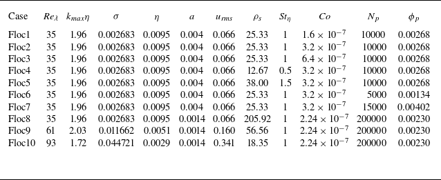
, respectively. We conducted 10 simulations to explore the effects of these factors on the evolution of flocs. The dimensionless parameters of simulations are listed in table 1.
Dimensionless parameters of simulations:
 ${\textit{Re}} \! = \! L_0U_0/\nu$
is the reciprocal of dimensionless kinematic viscosity, which is set to
 ${\textit{Re}}=5000$
;
 $N_p$
is the number of primary particles introduced into the flow field; and
 $\phi _p$
is the particle volume fraction. The resolution
 $k_{ {\textit{max}}} \eta$
exceeds 1.5 in all cases, satisfying the criterion for adequately resolving the smallest scales.

2.4. Identification and tracking of flocs
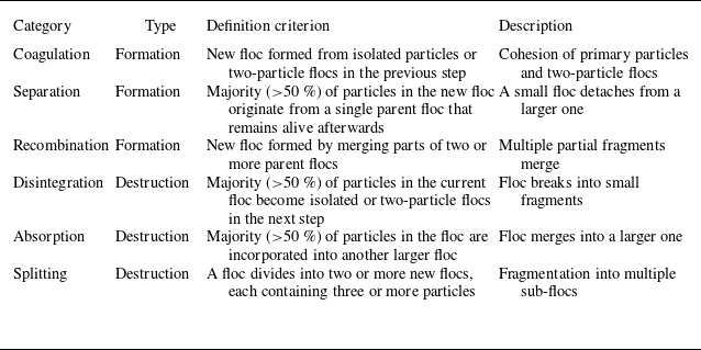
Primary particles are randomly introduced into the flow field after the flow has become statistically stationary. Two primary particles are considered as part of the same floc if their surface distance is smaller than half the range of the cohesive force (Zhao et al. Reference Zhao, Pomes, Vowinckel, Hsu, Bai and Meiburg2021). Throughout the paper, each individual primary particle is regarded as the smallest floc. However, to ensure a meaningful analysis, only formation and destruction of flocs composed of three or more primary particles are included in the evaluation.
The time interval between successive time steps is set to
 $0.5\tau _\eta$
, which is significantly shorter than that used by Zhao et al. (Reference Zhao, Pomes, Vowinckel, Hsu, Bai and Meiburg2021), and is sufficient to capture the detailed evolution of flocs. Following the approach of analysing clusters of non-cohesive particles in turbulence (Liu et al. Reference Liu, Shen, Zamansky and Coletti2020), two flocs in consecutive time steps are identified as successive realisations of the same floc if the fraction of shared particles exceeds 0.5 in both forward-in-time and backward-in-time connections. This is illustrated in figure 1(b): floc C shares two-thirds of its particles with floc E, and floc E shares all of its particles with floc C, resulting in forward and backward connection fractions 0.67 and 1, respectively. In contrast, floc C shares only one-third of its particles with floc D, and floc D shares all of its particles with floc C, yielding the forward and backward connection fractions between flocs C and D as 0.33 and 1, respectively. As a result, flocs C and E are identified as the same floc, meaning that the floc is considered ‘alive’ across these two time steps.
Schematic illustration of different types of formation of flocs: (a) coagulation, (b) separation, (c) recombination. The blue colour indicates the member particles at the previous time step, while the yellow colour represents the current time step. The analysis is limited to the formation of flocs comprising three or more primary particles.

Schematic illustration of different types of destruction of flocs: (a) disintegration, (b) absorption, (c) splitting. The blue colour indicates the member particles at the previous time step, while the yellow colour represents the current time step. Only the destruction of flocs containing at least three primary particles is analysed.

According to this tracking rule, the formation of flocs can originate from three types of events: coagulation, separation and recombination, as illustrated in figure 1. Specifically, coagulation refers to the formation of a new floc from individual primary particles or two-particle flocs in the previous time step, as seen with flocs A and B in figure 1(a). Separation refers to the case where a single parent floc contributes more than half of the particles in the newly formed floc, as in the case of floc D separating from floc C in figure 1(b). Recombination describes the merging of parts of multiple parent flocs to form a new one, as demonstrated by floc F in figure 1(c). Analogously, the causes of the destruction are categorised into three types: disintegration, absorption and splitting. Disintegration occurs if the majority of the particles from a floc become isolated parimary particles or two-particle flocs in the next time step, as seen with flocs G and H in figure 2(a). Absorption refers to a floc destructing when the majority of its particles are absorbed by another particle floc, such as floc I in figure 2(b). Splitting refers to the case where a floc divides into multiple new flocs, such as floc L in figure 2(c). To illustrate these processes further: in figure 1(b), floc D forms through the separation of floc C, which remains alive in the next time step. In contrast, in figure 2(b), floc I is absorbed by floc J and ceases to exist thereafter. It is also important to distinguish the focus of different subfigures. In figure 1(c), the emphasis is on the formation of floc F, which has just emerged. In comparison, figure 2(b) highlights the destruction of floc I through absorption. Although the processes shown in figures 1(b) and 2(c) are similar in nature, the former focuses on the formation of floc D, while the latter emphasises the destruction of floc L through splitting.
Finally, the lifetime of an individual floc,
 $t_{\mathit{life}}$
, is defined as the duration between its formation and subsequent destruction. For clarity, table 2 summarises the criteria to classify different types of floc formation and destruction events.
Definition and identification criteria for different types of floc formation and destruction events.

3. Results
In this section, the effects of cohesive strength, particle inertia, turbulent shear and particle volume fraction on various aspects of flocs – including the statistical properties of the formed flocs, the types of their formation and destruction, and their corresponding lifetimes – are analysed. The analysis is performed throughout the entire flocculation process, from the developing stage to the steady state.
3.1. Statistics of flocs
Temporal evolution of the number of flocs
 $N_{\! f}$
(normalised by the respective number of primary particles for each case) under different conditions: (a) varying cohesive number
 ${\textit{Co}}$
, with
 ${\textit{St}}_\eta = 1$
,
 ${\textit{Re}}_\lambda =35$
and
 $\phi _p = 0.00268$
; (b) varying Reynolds number
 ${\textit{Re}}_\lambda$
, with
 ${\textit{St}}_\eta = 1$
,
 ${\textit{Co}}=2.24\times 10^{-7}$
and
 $\phi _p = 0.00230$
; (c) varying Stokes number
 ${\textit{St}}_\eta$
, with
 ${\textit{Re}}_\lambda =35$
,
 ${\textit{Co}}=3.2\times 10^{-7}$
and
 $\phi _p = 0.00268$
; (d) varying particle volume fractions
 $\phi _p$
, with
 ${\textit{Re}}_\lambda =35$
,
 ${\textit{St}}_\eta = 1$
and
 ${\textit{Co}}=3.2\times 10^{-7}$
.

First, the effects of various factors on the temporal evolution of the number of flocs
 $N_{\! f}$
are depicted in figure 3. Since each primary particle is considered the smallest floc, the initial number of flocs equals the total number of primary particles. Across all conditions, the flocculation process consistently proceeds in two distinct stages: an rapid initial reduction in the number of flocs, followed by a gradual levelling off. This behaviour indicates that starting with individual primary particles, the flocculation process transitions through a developing stage before reaching a statistically steady stage, consistent with findings from previous studies (Moussa et al. Reference Moussa, Soos, Sefcik and Morbidelli2007; Wang et al. Reference Wang, Nan, Ji and Yang2018; Zhao et al. Reference Zhao, Vowinckel, Hsu, Köllner, Bai and Meiburg2020, Reference Zhao, Pomes, Vowinckel, Hsu, Bai and Meiburg2021; Yu et al. Reference Yu, Yu and Balachandar2022b
).
In figure 3(a), particles with stronger cohesive strength lead to a lower number of flocs, indicating that each floc contains more primary particles. In other words, flocs with stronger cohesive strength are more resistant to the turbulent shear imposed by the flow field, allowing them to grow to a larger size. Consequently, flocs with the same cohesive strength but exposed to higher turbulent shear will be smaller, as indicated by the increase in the number of flocs with increasing Reynolds number in figure 3(b). The use of a relatively low
 ${\textit{Re}}_\lambda =35$
follows Zhao et al. (Reference Zhao, Pomes, Vowinckel, Hsu, Bai and Meiburg2021), in which the calibrated flocculation model based on simulation results showed a good agreement with experimental results. This allows physically meaningful parametric studies at an affordable computational cost. Although a higher
 ${\textit{Re}}_\lambda$
turbulent flow enhances floc break-up, an additional test at
 ${\textit{Re}}_\lambda =93$
demonstrates that increasing the cohesion number can still sustain the population of larger flocs, indicating that flocculation is not completely suppressed at relatively high Reynolds numbers. A particularly interesting outcome is observed in figure 3(c), where particles with weak inertia tend to form larger flocs at steady state (Zhao et al. Reference Zhao, Pomes, Vowinckel, Hsu, Bai and Meiburg2021). A plausible explanation for this phenomenon is that particles with weak inertia can follow the fluid motion more faithfully, enabling them to remain together and grow in size. Zhao et al. (Reference Zhao, Pomes, Vowinckel, Hsu, Bai and Meiburg2021) reported that flocs composed of particles with Stokes number
 ${\textit{St}}_\eta =1$
exhibit the fastest growth during the early development stage when using a three-way coupling framework. This behaviour arises because particles with
 ${\textit{St}}_\eta =1$
experience the most intense preferential accumulation (Wang & Maxey Reference Wang and Maxey1993; Balachandar & Eaton Reference Balachandar and Eaton2010), which enhances clustering and promotes adhesion. When four-way coupling is adopted, the particle feedback on the fluid alters the local flow structures and reduces the strength of preferential concentration. As a result, the rapid early growth observed at
 ${St}_\eta =1$
under three-way coupling no longer appears.
Figure 3(d) illustrates how particle volume fraction influences the temporal evolution of the total number of flocs. As the particle volume fraction increases, the number of flocs systematically decreases, and the system approaches its equilibrium state more rapidly. This behaviour stems from the higher particle concentration, which directly increases the likelihood of particle–particle collisions, thereby accelerating the flocculation process. As a result, more frequent early-stage flocculation not only reduces the final number of flocs, but also leads the system to reach a statistically steady state in less time.
Probability density functions (PDFs) of the number of primary particles
 $n_{\!f}$
contained in individual flocs at steady state under different conditions are illustrated in figure 4. It can be observed that a significant number of primary particles remain at steady state, while the number of flocs decreases as their size increases, a trend that aligns with previous investigations (Zhao et al. Reference Zhao, Pomes, Vowinckel, Hsu, Bai and Meiburg2021; Yu et al. Reference Yu, Yu, Balachandar and Manning2022b
). As discussed earlier with respect to figure 3(a), particles with stronger cohesive strength tend to form larger flocs, as also demonstrated in figure 4(a). Similarly, particles with weaker inertia or those exposed to weaker turbulent shear tend to form larger flocs, as shown in figures 4(b) and 4(c). In addition, higher particle volume fraction facilitates the formation of larger flocs, as shown in figure 4(d). Yu et al. (Reference Yu, Yu, Balachandar and Manning2022b
) observed that the equilibrium floc size distribution has an asymmetric shape with a peak, a feature not seen in the current simulation results. This suggests that the equilibrium floc size distribution is highly dependent on the properties of particles and the characteristics of the underlying flow field.
The PDFs of the numbers of primary particles contained in flocs at steady state under different conditions: (a) varying cohesive number
 ${\textit{Co}}$
, with
 ${\textit{St}}_\eta = 1$
,
 ${\textit{Re}}_\lambda =35$
and
 $\phi _p = 0.00268$
; (b) varying Reynolds number
 ${\textit{Re}}_\lambda$
, with
 ${\textit{St}}_\eta = 1$
,
 ${\textit{Co}}=2.24\times 10^{-7}$
and
 $\phi _p = 0.00230$
; (c) varying Stokes number
 ${\textit{St}}_\eta$
, with
 ${\textit{Re}}_\lambda =35$
,
 ${\textit{Co}}=3.2\times 10^{-7}$
and
 $\phi _p = 0.00268$
; (d) varying particle volume fractions
 $\phi _p$
, with
 ${\textit{Re}}_\lambda =35$
,
 ${\textit{St}}_\eta = 1$
and
 ${\textit{Co}}=3.2\times 10^{-7}$
.

The PDFs of the averaged fractal dimensions of individual flocs throughout their lifetime under different conditions: (a) varying cohesive number
 ${\textit{Co}}$
, with
 ${\textit{St}}_\eta = 1$
,
 ${\textit{Re}}_\lambda =35$
and
 $\phi _p = 0.00268$
; (b) varying Reynolds number
 ${\textit{Re}}_\lambda$
, with
 ${\textit{St}}_\eta = 1$
,
 ${\textit{Co}}=2.24\times 10^{-7}$
and
 $\phi _p = 0.00230$
; (c) varying Stokes number
 ${\textit{St}}_\eta$
, with
 ${\textit{Re}}_\lambda =35$
,
 ${\textit{Co}}=3.2\times 10^{-7}$
and
 $\phi _p = 0.00268$
; (d) varying particle volume fractions
 $\phi _p$
, with
 ${\textit{Re}}_\lambda =35$
,
 ${\textit{St}}_\eta = 1$
and
 ${\textit{Co}}=3.2\times 10^{-7}$
.

We then examine the compactness of the formed flocs at the steady state. The compactness is quantified by the fractal dimension
 $d_{\!f}$
of floc, given by (Zhao et al. Reference Zhao, Pomes, Vowinckel, Hsu, Bai and Meiburg2021)
 \begin{equation} d_{\!f} = \frac {\log n_{\! f}}{\log ({D_{\!f}}/{D_{\!p}})}, \end{equation}
where
 $D_{\!p}$
is the diameter of the primary particle, and
 $D_{\! f}$
is the characteristic diameter of the floc, defined as
 \begin{equation} D_{\!f} = 2 \max(\|\boldsymbol{x}_{p,i}-\boldsymbol{x}_{c}\|)+D_{\!p}, \quad 1 \leqslant i \leqslant n_{\!f}. \end{equation}
In this expression,
 $\boldsymbol{x}_{p,i}$
represents the position of the centre of primary particle
 $i$
, and the centre of mass of floc is calculated as
 $\boldsymbol{x}_{c} =\sum _{ i=1}^{n_{\!f}}\boldsymbol{x}_{p,i}/n_{\!f}$
. A dense, nearly spherical floc typically has fractal dimension close to
 $d_{\! f} \approx 3$
, while a linear, chain-like floc has a much lower value,
 $d_{\! f} \approx 1$
. In principle, the fractal dimension of flocs ranges from 1 to 3, with higher values corresponding to more compact and tightly packed structures. Note that the fractal dimension here is employed as an indicator to characterise the compactness of flocs, regardless of large flocs of many member particles or small flocs consisting of only a few (e.g. 3–4) particles.
The PDFs of the averaged fractal dimensions of individual flocs throughout their lifetime (denoted by the angle bracket
 $\left \langle \right \rangle$
) are displayed in figure 5. The statistics for the fractal dimension are conducted only for flocs containing three or more primary particles. The range of fractal dimension aligns with the ranges reported in previous studies (Chen et al. Reference Chen, Li and Marshall2019; Zhao et al. Reference Zhao, Pomes, Vowinckel, Hsu, Bai and Meiburg2021). The PDF distribution clearly exhibits two distinct peaks at values 1.0 and 1.4, indicating two characteristic floc structures, as will be discussed further below. In figure 5(a), under identical turbulent shear and particle inertia, flocs with stronger cohesive strength are more likely to attain higher fractal dimension values, reflecting a more compact structure. As indicated in figure 4(a), particles with stronger cohesive strength can form larger flocs. This is because more compact flocs can better withstand turbulent shear and maintain their size, and serve as building blocks for the formation of even larger flocs. Similarly, particles with weaker inertia or those subjected to lower turbulent shear tend to form flocs with a more compact structure (figures 5
b,c). Figure 5(d) further indicates that changing the particle volume fraction produces distributions that are nearly identical, with the only noticeable difference being a slightly more compact structure in the case with a higher particle volume fraction. These findings suggest that factors such as cohesive strength, particle inertia and turbulent shear can be adjusted to achieve flocs with desired compactness.
Averaged numbers of primary particles contained in flocs, conditioned on the average fractal dimension, under different conditions: (a) varying cohesive number
 ${\textit{Co}}$
, with
 ${\textit{St}}_\eta = 1$
,
 ${\textit{Re}}_\lambda =35$
and
 $\phi _p = 0.00268$
; (b) varying Reynolds number
 ${\textit{Re}}_\lambda$
, with
 ${\textit{St}}_\eta = 1$
,
 ${\textit{Co}}=2.24\times 10^{-7}$
and
 $\phi _p = 0.00230$
; (c) varying Stokes number
 ${\textit{St}}_\eta$
, with
 ${\textit{Re}}_\lambda =35$
,
 ${\textit{Co}}=3.2\times 10^{-7}$
and
 $\phi _p = 0.00268$
; (d) varying particle volume fractions
 $\phi _p$
, with
 ${\textit{Re}}_\lambda =35$
,
 ${\textit{St}}_\eta = 1$
and
 ${\textit{Co}}=3.2\times 10^{-7}$
.

To further clarify the peaks in the PDFs of the fractal dimension of flocs, the average number of primary particles contained in the flocs, conditioned on the average fractal dimension, is presented in figure 6. Interestingly, the conditioned average number of particles exhibits a noticeable dip at the fractal dimension values corresponding to the peaks in the PDF distribution. The valley at fractal dimension value 1.0 corresponds to an average number of three particles, indicating a linear structure of flocs consisting of three particles. Meanwhile, the valley at fractal dimension 1.4 corresponds to a narrow range of average particle numbers between 3.0 and 4.5, which suggests small flocs with a planar distribution structure. These results indicate that typical floc sizes are associated with some characteristic structures. Furthermore, larger fractal dimensions are generally associated with larger flocs, confirming that flocs with a more compact structure tend to grow more easily in size. In conclusion, weaker turbulent shear, lower particle inertia and stronger cohesive strength all contribute to the formation of larger and more compact flocs.
3.2. Formation and destruction of flocs
In this subsection, we delve into the different types of floc formation and destruction to better understand the underlying dynamics of flocculation. The rapid initial reduction stage before the system enters the equilibrium stage in § 3.1 is further divided into two stages, i.e. the early flocculation stage and the transition stage. Therefore, three distinct stages are identified here: the early flocculation stage, the transition stage and the equilibrium stage. This classification of stages is illustrated in figure 1(a), where the dashed line marks the separation between the stages. This refined classification can provide more detailed insights into the dynamics of flocculation process (Wang et al. Reference Wang, Nan, Ji and Yang2018).
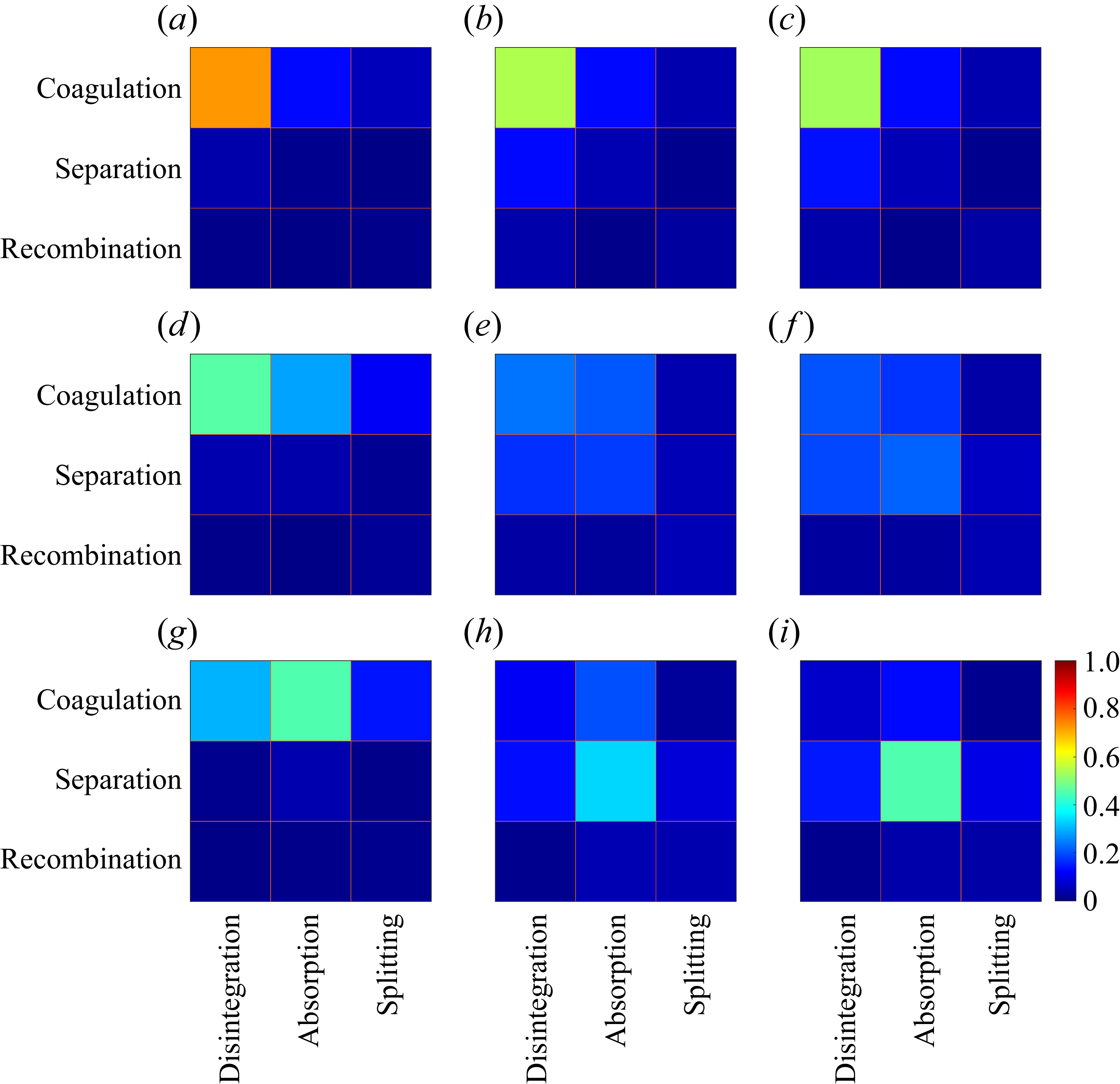
Probability of different floc formation and destruction types at various stages under different cohesion numbers: (a,b,c)
 ${\textit{Co}}=1.6\times 10^{-7}$
, (d,e, f)
 ${\textit{Co}}=3.2\times 10^{-7}$
, (g,h,i)
 ${\textit{Co}}=6.4\times 10^{-7}$
. Early flocculation stage in (a,d,g); transition stage in (b,e,h); equilibrium stage in (c, f,i). The Stokes number is
 ${St}_\eta =1.0$
, the Reynolds number is
 ${\textit{Re}}_\lambda =35$
, and the particle volume fraction is
 $\phi _p = 0.00268$
.

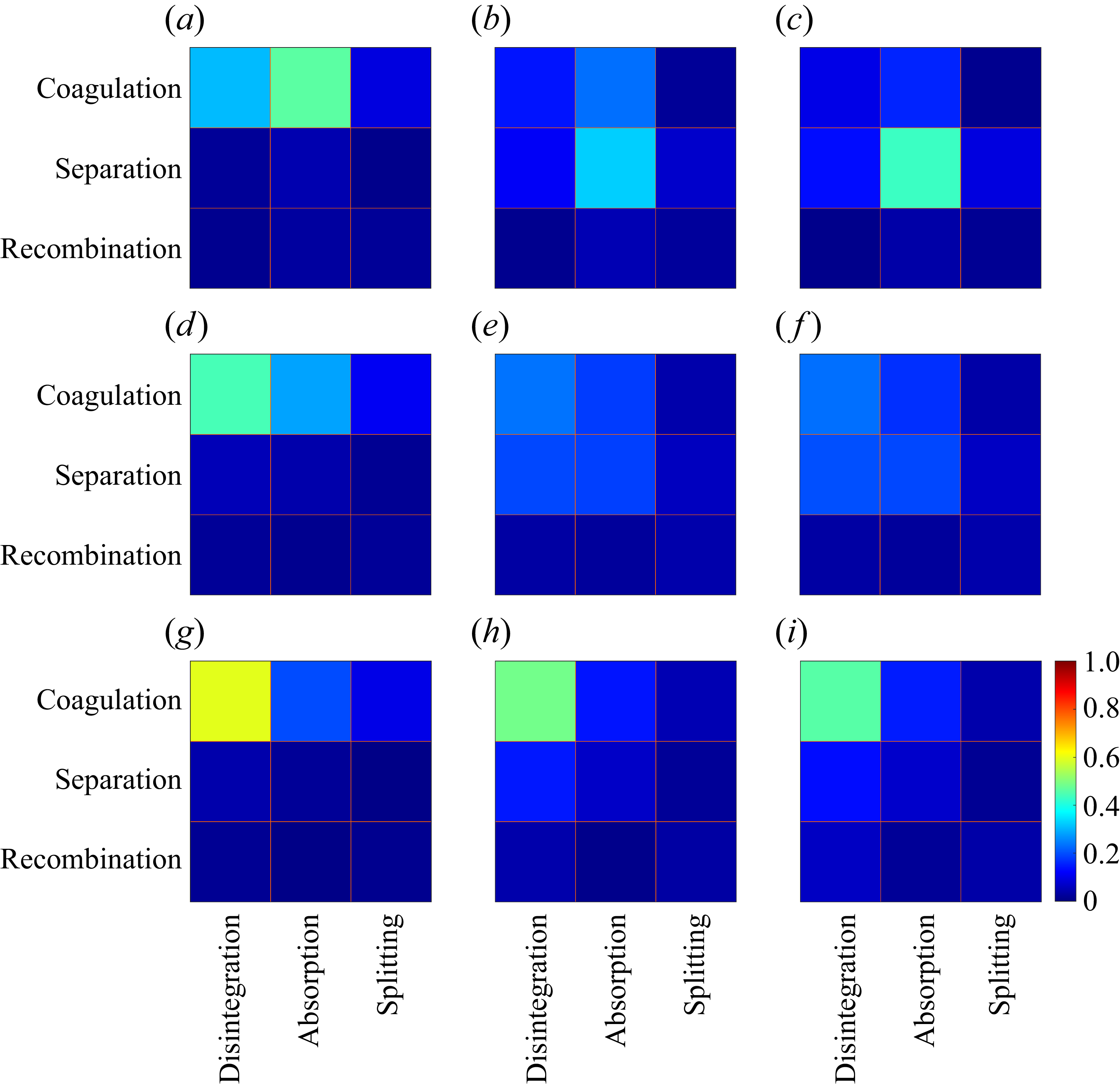
Probability of different floc formation and destruction types at various stages under different Reynolds numbers: (a,b,c)
 ${\textit{Re}}_\lambda =35$
, (d,e, f)
 ${\textit{Re}}_\lambda =61$
, (g,h,i)
 ${\textit{Re}}_\lambda =93$
. Early flocculation stage in (a,d,g); transition stage in (b,e,h); equilibrium stage in (c, f,i). The cohesive number is
 ${\textit{Co}}={6.4\times 10}^{-7}$
, the Stokes number is
 ${St}_\eta =1.0$
, and the particle volume fraction is
 $\phi _p = 0.00230$
.

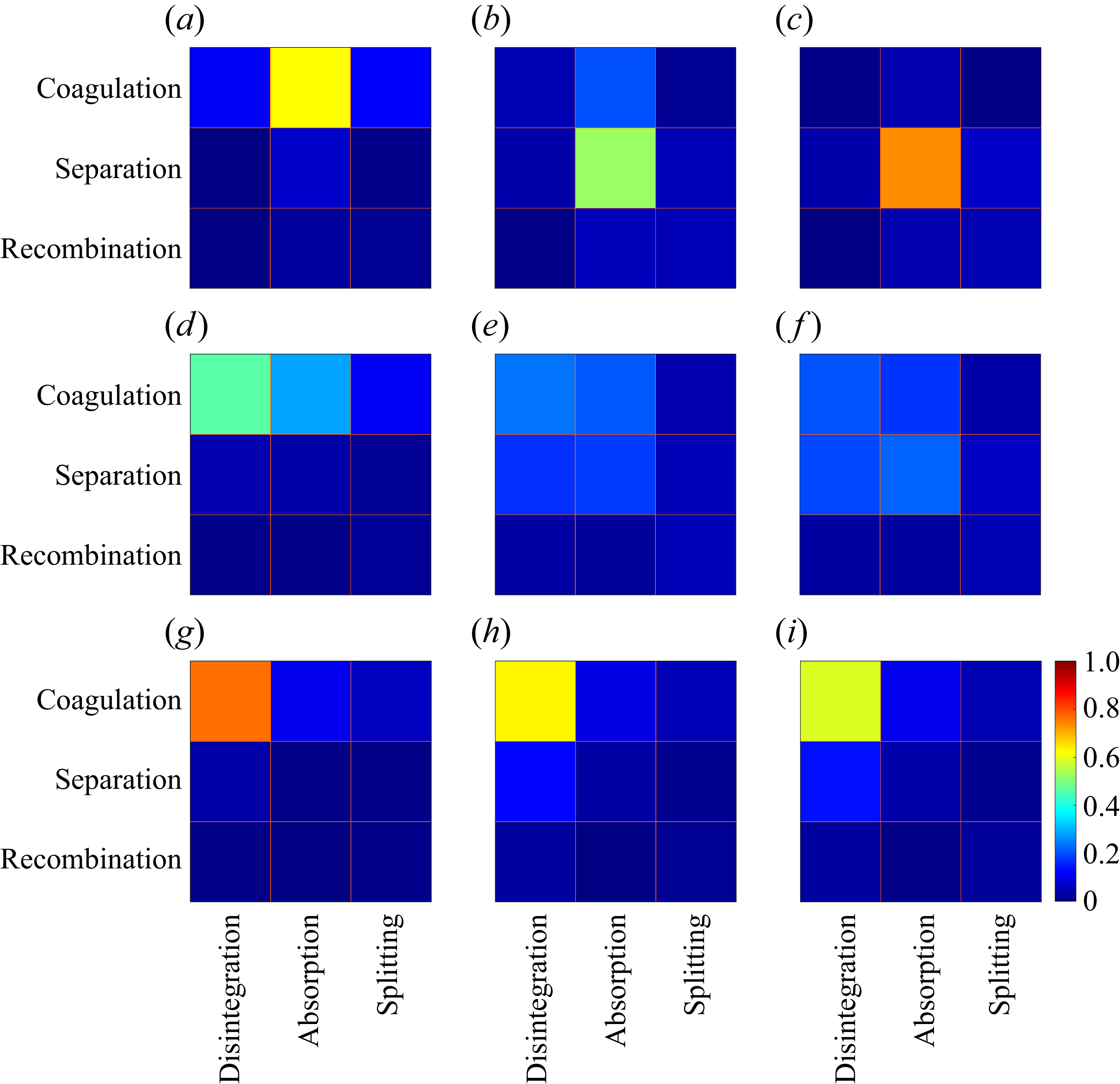
Figure 7 illustrates the probabilities of various combinations of floc formation and destruction types across different stages at various cohesion numbers. It is evident that the types of floc formation and destruction change with the cohesive strength at different flocculation stages. Regardless of the cohesive strength, flocs initially form through coagulation, as most particles not belonging to any flocs in the previous time step begin to aggregate at the early flocculation stage. This is because the flocculation process begins with individual primary particles. As time progresses, however, the dominant mode of floc formation changes and is dependent on the cohesion number. When the cohesive strength is relatively weak, most flocs continue to form through coagulation, with only a small fraction forming through separation. In contrast, as cohesive strength gradually increases, floc formation by separation becomes more prominent during the transition stage, and ultimately dominates during the equilibrium stage (see figure 7 i). Regarding the destruction process, flocs are mainly eliminated by disintegration across all stages when the cohesive strength is relatively weak, but through absorption when the cohesive strength is strong enough. For the intermediate cohesive strength, the mode of destruction shifts from a combination of disintegration and absorption at the early flocculation stage to absorption during the equilibrium stage. These shifts in the types of floc formation and destruction can be explained as follows. Flocs with weak cohesive strength cannot resist the turbulent shear and thus disintegrate into particles during the early flocculation stage, with mostly primary particles acting as building blocks for flocs across all stages. In contrast, flocs with strong cohesive strength are better able to withstand turbulent shear, allowing them to serve as building blocks for larger flocs via absorption. When flocs grow beyond a certain size, further growth is limited by turbulence. Due to the strong cohesion, they do not undergo splitting into multiple smaller flocs; instead, only relatively small flocs can detach from their surface, resulting in separation (Frungieri & Vanni Reference Frungieri and Vanni2021). This also suggests that modes of absorption and separation are interrelated, with absorption as a prerequisite for the occurrence of separation. Statistically, separation tends to occur only when absorption events are sufficiently frequent, because absorption promotes the growth of parent flocs from which daughter flocs can detach.
Probability of different floc formation and destruction types at various stages under different Stokes numbers: (a,b,c)
 ${St}_\eta =0.5$
, (d,e, f)
 ${St}_\eta =1.0$
, (g,h,i)
 ${St}_\eta =1.5$
. Early flocculation stage in (a,d,g); transition stage in (b,e,h); equilibrium stage in (c, f,i). The cohesive number is
 ${\textit{Co}}={3.2\times 10}^{-7}$
, the Reynolds number is
 ${\textit{Re}}_\lambda =35$
, and the particle volume fraction is
 $\phi _p = 0.00268$
.

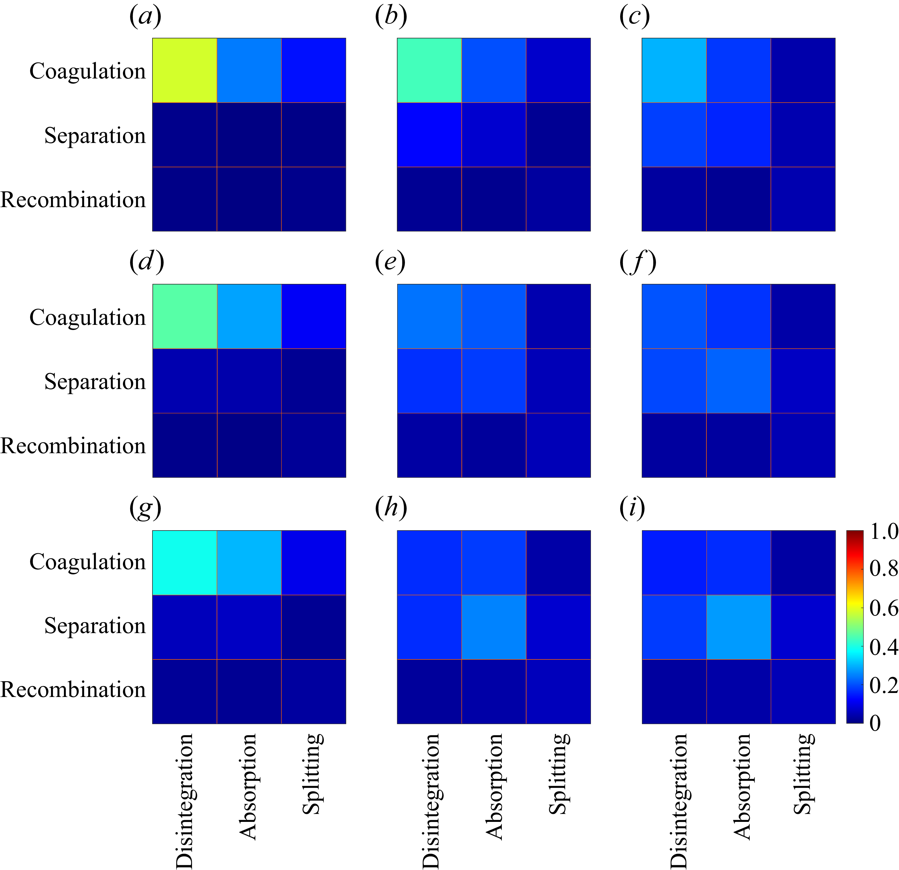
The probabilities of various combinations of formation and destruction types for flocs at different stages and under varying Reynolds numbers are shown in figure 8. Similar to the observations in figure 7, flocs are initially formed through coagulation at the early flocculation stage, irrespective of the Reynolds number. When the Reynolds number is low, the formation of flocs gradually shifts from coagulation to separation over time. However, for high Reynolds numbers, flocs continue to form predominantly through coagulation from individual primary particles, in line with the size distribution observed in figure 3(b). The dependence of formation of flocs on Reynolds number suggests that flocs in lower Reynolds number turbulence persist longer and grow larger in size. This is further supported by the floc destruction: flocs are primarily eliminated through absorption at low Reynolds numbers, indicating that small flocs can further aggregate into larger flocs; however, flocs mainly disintegrate at high Reynolds numbers, resulting in only small flocs. Furthermore, these observations confirm that absorption is a prerequisite for the occurrence of separation, as illustrated in figures 8(a,b,c). Therefore, stable and compact small flocs are essential for the formation of larger flocs.
Figure 9 illustrates the probabilities of floc formation and destruction types at varying Stokes numbers. We can observe that flocs tend to form through coagulation at the early stage, and later shift to separation at the equilibrium stage, at small Stokes number. In contrast, for large Stokes number, flocs are mainly formed through coagulation throughout the entire process. This observation suggests the longer lifetime and larger size of flocs composed of less-inertial particles in turbulent flows. The destruction of flocs further supports this observation, with flocs primarily breaking up through absorption for small Stokes numbers, and through disintegration for large Stokes number. Similarly, as the particle inertia increases, there is a noticeable shift from absorption to disintegration in the destruction mode of flocs. In addition, a similar trend is observed with increasing the turbulent shear and particle inertia (figures 8 and 9).
Probability of different floc formation and destruction types at various stages under different particle volume fractions: (a,b,c)
 $\phi _p=0.00134$
, (d,e, f)
 $\phi _p=0.00268$
, (g,h,i)
 $\phi _p=0.00402$
. Early flocculation stage in (a,d,g); transition stage in (b,e,h); equilibrium stage in (c, f,i). The cohesive number is
 ${\textit{Co}}={3.2\times 10}^{-7}$
, the Stokes number is
 ${\textit{St}}_\eta =1$
, and the Reynolds number is
 ${\textit{Re}}_\lambda =35$
.

Figure 10 shows the probabilities of different floc formation and destruction types at various stages under different particle volume fractions. As particle volume fraction increases, these probabilities transition in a pattern similar to that observed with increased cohesion strength (see figure 7), but the effect is weaker. Figure 10 also indicates that a higher particle volume fraction increases the frequency of particle–particle encounters, altering the dominant formation and destruction mechanisms during the steady stage.
In summary, the types of floc formation and destruction vary across different flocculation stages, and are influenced by cohesive strength, turbulent shear, particle inertia and particle volume fraction. At the early stage, flocs consistently form through coagulation. In contrast, during the equilibrium stage, both coagulation and separation contribute to floc formation. Coagulation is favoured under conditions of weak cohesive strength, strong turbulent shear, large particle inertia and small particle volume fraction, while separation tends to dominate under the opposite conditions. The destruction of flocs may occur through disintegration or absorption, with these modes either remaining constant or changing across stages depending on the conditions. Under weak cohesive strength, high particle inertia, strong turbulent shear or small particle volume fraction, the destruction of flocs occurs mainly through disintegration across all stages. In contrast, with increasing cohesive strength, decreasing particle inertia, decreasing turbulent shear or increasing particle volume fraction, floc destruction shifts to absorption. Importantly, there exists a competing effect among cohesive strength, turbulent shear and particle inertia in governing the formation and destruction of flocs, with a similar trend observed between the particle inertia and turbulent shear.
A comparison with the non-cohesive particle cluster dynamics reported by Liu et al. (Reference Liu, Shen, Zamansky and Coletti2020) reveals some interesting similarities. They found that the most common scenarios for particle clusters are the birth by coagulation and the death by disintegration, while birth by recombination and death by splitting occur less frequently. These patterns are also observed for flocs at the equilibrium stage (figures 7(c), 8(i) and 9(i)). However, formation by separation and destruction by absorption are also prevalent for the flocculation dynamics (figures 7(i), 8(c) and 9(c)), indicating that cohesive bonds between primary particles play a significant role in influencing the dynamics of the system. This distinction is expected to result in differences in the lifetime of flocs compared to clusters, which are discussed in the next subsection.
3.3. Lifetime of flocs
This subsection investigates the lifetime of flocs,
 $t_{\mathit{life}}$
, defined as the duration between its formation and subsequent destruction, as described in § 2.4.
The PDFs of the floc lifetime for different cases: (a) varying cohesive number
 ${\textit{Co}}$
with
 ${\textit{St}}_\eta = 1$
,
 ${\textit{Re}}_\lambda =35$
and
 $\phi _p = 0.00268$
; (b) varying Reynolds number
 ${\textit{Re}}_\lambda$
with
 ${\textit{St}}_\eta = 1$
,
 ${\textit{Co}}=2.24\times 10^{-7}$
and
 $\phi _p = 0.00230$
; (c) varying Stokes number
 ${\textit{St}}_\eta$
with
 ${\textit{Re}}_\lambda =35$
,
 ${\textit{Co}}=3.2\times 10^{-7}$
and
 $\phi _p = 0.00268$
; (d) varying particle volume fractions
 $\phi _p$
with
 ${\textit{Re}}_\lambda =35$
,
 ${\textit{St}}_\eta = 1$
and
 ${\textit{Co}}=3.2\times 10^{-7}$
.

Figure 11 shows the PDFs of floc lifetime for the different cases. It is evident that these PDFs exhibit an exponential decay as
 $t_{\mathit {life}}$
increases. This suggests the difficulty for particle flocs to survive for a long time in turbulence. From figure 11(a), it can be observed that the floc lifetime increases with the cohesion number
 ${\textit{Co}}$
. This is attributed to the stronger cohesive bonds to resist the floc break-up, thereby extending the existence of flocs. Conversely, figure 11(b) shows that floc lifetime decreases with
 ${\textit{Re}}_{\lambda }$
, owing to the intensified turbulent shear that promotes floc disruption.
A similar decay in persistence has also been studied for non-cohesive particle clusters. For instance, Liu et al. (Reference Liu, Shen, Zamansky and Coletti2020) investigated the lifetime of non-cohesive particle clusters, and found increased cluster lifetime as the Stokes number rises. This is because particles with larger inertia are less responsive to turbulent fluctuations, and once brought into proximity, tend to remain close to one another due to their own inertia, leading to longer-lived clusters. In contrast, as shown in figure 11(c), an opposite trend is observed for floc lifetime, which decreases with increasing Stokes number. This opposite trend arises from both the different definitions and different physical mechanisms governing clusters and flocs. While clusters are identified based on spatial proximity alone, flocs are defined by the presence of cohesive bonds between particles. Although inertial particles may stay close to each other, the cohesive bonds between them are more easily broken due to stronger relative motion. Consequently, flocs formed under high-inertia conditions are more prone to bond breakage, leading to shorter lifetime despite the particles remaining nearby.
The effect of particle volume fractions on the PDFs of floc lifetime is presented in figure 11(d). The floc lifetime decreases as the particle volume fraction
 $\phi _p$
increases, a trend that may seem counterintuitive. Although a larger particle volume fraction leads to the formation of larger floc sizes, as shown in figure 4(d), and larger flocs generally exhibit longer lifetimes under different parameters (figures 11
a–c), increasing
 $\phi _p$
introduces two opposing effects. First, more particles result in a higher encounter frequency, promoting the formation of larger, more compact flocs, as supported by the conditional average fractal dimension discussed later. These features tend to increase the typical floc size, and would favour longer-lived flocs. Second, intensified particle interactions increase the frequency of collisions, facilitating the exchange of primary particles among flocs, and in turn, more fragmentation events that end the lifetime of existing flocs and generate new ones. As
 $\phi _p$
increases, these disruptive events become more frequent, offsetting the stabilising effect associated with the formation of large and compact flocs. Thus although the system contains larger flocs on average, the lifespan of individual flocs is shortened because the higher collision frequency accelerates floc destruction.
The averaged floc lifetime for each combination of different types of floc formation and destruction at the steady stage for different cases: (a,b,c) varying cohesive number
 ${\textit{Co}}$
, with
 ${\textit{St}}_\eta = 1$
,
 ${\textit{Re}}_\lambda = 35$
and
 $\phi _p = 0.00268$
; (d,e, f) varying Reynolds number
 ${\textit{Re}}_\lambda$
, with
 ${\textit{St}}_\eta = 1$
,
 ${\textit{Co}} = 6.4\times 10^{-7}$
and
 $\phi _p = 0.00230$
; (g,h,i) varying Stokes number
 ${\textit{St}}_\eta$
, with
 ${\textit{Re}}_\lambda = 35$
,
 ${\textit{Co}} = 3.2\times 10^{-7}$
and
 $\phi _p = 0.00268$
; (j, k,l) varying particle volume fraction
 $\phi _p$
, with
 ${\textit{Re}}_\lambda = 35$
,
 ${\textit{St}}_\eta = 1$
and
 ${\textit{Co}} = 3.2\times 10^{-7}$
. The averaged floc lifetimes are normalised by the maximum across all combinations.

Averaged characteristic diameter of flocs conditioned on the floc lifetime for different cases: (a) varying cohesive number
 ${\textit{Co}}$
, with
 ${\textit{St}}_\eta = 1$
,
 ${\textit{Re}}_\lambda =35$
and
 $\phi _p = 0.00268$
; (b) varying Reynolds number
 ${\textit{Re}}_\lambda$
, with
 ${\textit{St}}_\eta = 1$
,
 ${\textit{Co}}=2.24\times 10^{-7}$
and
 $\phi _p = 0.00230$
; (c) varying Stokes number
 ${\textit{St}}_\eta$
, with
 ${\textit{Re}}_\lambda =35$
,
 ${\textit{Co}}=3.2\times 10^{-7}$
and
 $\phi _p = 0.00268$
; (d) varying particle volume fraction
 $\phi _p$
, with
 ${\textit{Re}}_\lambda =35$
,
 ${\textit{St}}_\eta = 1$
and
 ${\textit{Co}}=3.2\times 10^{-7}$
.

Another notable difference between the lifetimes of flocs and clusters is that cohesive bonds can significantly extend the lifetimes of flocs. As shown in figure 11, the lifetimes of flocs are typically of the order of hundreds of Kolmogorov time scales, whereas for clusters, the lifetimes are generally of the order of tens of Kolmogorov time scales (Liu et al. Reference Liu, Shen, Zamansky and Coletti2020). This longer time scale for floc lifetime is consistent with the findings of Frungieri et al. (Reference Frungieri, Bäbler, Biferale and Lanotte2023). They introduced aggregates into turbulence and tracked their trajectories, recording the total hydrodynamic stress along the path of each aggregate. They assumed that aggregates would break up intermediately when the hydrodynamic stress exceeded a predefined critical value. The time between the release of the aggregate and its break-up was defined as the exit time, which can be considered as the lifetime of the aggregates. They observed that the exit time is approximately exponentially distributed and of the order of hundreds of Kolmogorov time scales, consistent with the findings of the present study. Owing to the use of the same Lagrangian framework in Babler et al. (Reference Babler2015) and Frungieri et al. (Reference Frungieri, Bäbler, Biferale and Lanotte2023), and the close agreement between Frungieri et al. (Reference Frungieri, Bäbler, Biferale and Lanotte2023) and the present simulations, our findings indirectly support the claim by Babler et al. (Reference Babler2015). Specifically, floc break-up occurs when local hydrodynamic stress is proportional to the square root of the energy dissipation, and break-up rates can be inferred from tracking the temporal evolution of the aggregate number.
The exponential decay observed in the PDFs of floc lifetime resembles that reported for the lifetime of vortex filaments in homogeneous isotropic turbulence (Biferale, Scagliarini & Toschi Reference Biferale, Scagliarini and Toschi2010). However, there is no evidence of a causal connection between these two processes. The heavy particles under current study exhibit preferential sampling in strain-dominated regions rather than vortex filaments. Moreover, the lifetime of flocs spans several hundreds of
 $\tau _\eta$
, which is much longer than typical vortex-filament lifetime. Additionally, these two lifetimes also exhibit opposite Reynolds number dependence: long-lived vortex filaments are more probable at higher
 ${\textit{Re}}_\lambda$
, while flocs survive longer at lower
 ${\textit{Re}}_\lambda$
. These observations indicate that the exponential lifetime statistics of flocs arise from mechanisms different from those of vortex-filament dynamics.
Figure 12 shows the conditional-averaged floc lifetimes for all combinations of formation and destruction types during the statistically steady stage across the different cases. Flocs formed through separation and destroyed by splitting generally exhibit long lifetimes. Similarly, the combinations of coagulation with splitting, and recombination with absorption, can also lead to long lifetimes. The combination of recombination and absorption behaves differently with respect to cohesive strength and particle inertia. Specifically, increasing the cohesive strength results in longer lifetimes for this combination, whereas increasing particle inertia leads to shorter lifetimes.
Averaged fractal dimension of flocs conditioned on the floc lifetime for different cases: (a) varying cohesive number
 ${\textit{Co}}$
, with
 ${\textit{St}}_\eta = 1$
,
 ${\textit{Re}}_\lambda =35$
and
 $\phi _p = 0.00268$
; (b) varying Reynolds number
 ${\textit{Re}}_\lambda$
, with
 ${\textit{St}}_\eta = 1$
,
 ${\textit{Co}}=2.24\times 10^{-7}$
and
 $\phi _p = 0.00230$
; (c) varying Stokes number
 ${\textit{St}}_\eta$
, with
 ${\textit{Re}}_\lambda =35$
,
 ${\textit{Co}}=3.2\times 10^{-7}$
and
 $\phi _p = 0.00268$
; (d) varying particle volume fraction
 $\phi _p$
, with
 ${\textit{Re}}_\lambda =35$
,
 ${\textit{St}}_\eta = 1$
and
 ${\textit{Co}}=3.2\times 10^{-7}$
.

As shown in figure 12, the lifetimes of flocs are also found to be associated with how they are formed and destructed. Since other floc properties are also correlated with these specific combinations, it is anticipated that floc lifetime will be related to other floc properties as well, particularly the floc size and compactness. Figure 13 shows the average characteristic diameter of flocs conditioned on their lifetime for different cases. Clearly, stronger cohesive strength, weaker turbulent shear and low particle inertia lead to larger conditional average flocs. More importantly, no definite correlation between the conditional average characteristic diameter of flocs and their lifetime is observed. It is observed from figure 13(a) that the floc size and lifetime are positively correlated for the case with
 ${\textit{Co}}=6.4\times 10^{-7}$
, while they are negatively correlated for the case with
 ${\textit{Co}}=1.6\times 10^{-7}$
. However, Liu et al. (Reference Liu, Shen, Zamansky and Coletti2020) observed a positive correlation between cluster size and lifetime. This discrepancy between flocs and clusters further emphasises the significant role of cohesive bonds between primary particles in shaping the dynamics of the system. This also implies that the characteristic diameter of flocs is not a reliable indicator of their lifetime.
Figure 14 shows the average fractal dimension of flocs conditioned on the lifetime of flocs in the different cases. The dependence of the average fractal dimension on the cohesion number, Reynolds number, Stokes number and particle volume fraction exhibits the same tendency as observed in figure 5. Specifically, stronger turbulent shear, larger particle inertia, weaker cohesive strength and smaller particle volume fraction lead to less compact flocs (figure 5 a–c). When conditions such as cohesion number, particle inertia or turbulent shear favour floc formation, two consistent trends emerge: longer-lived flocs tend to be more compact, and these conditions also yield greater compactness when conditioned on a given lifetime. By contrast, increasing particle volume fraction also promotes floc formation by raising the frequency of particle encounters, but conditional statistics indicate only slightly higher compactness at a given lifetime, while overall floc lifetime decreases. This occurs because more frequent particle encounters both contribute to floc compaction and increase the likelihood of break-up. More importantly, it is evident that the average fractal dimension of flocs is positively correlated with their lifetime across all cases, although there is considerable scatter for long lifetime due to the limited samples. This positive relationship can be explained by the fact that more compact flocs are better able to resist break-up and thus have longer lifetime. Therefore, the fractal dimension, which reflects the compactness of flocs, can serve as a more reliable indicator for estimating the magnitude of floc lifetime.
4. Conclusions
In this study, we conducted direct numerical simulations coupled with a cohesive discrete element method to investigate the evolution of cohesive particle flocs in homogeneous isotropic turbulence. The discrete element method accounts for interactions among primary particles, including cohesion, lubrication and collision. The primary focus was on the effects of cohesive strength, particle inertia, turbulent shear and particle volume fraction on the properties and lifetime of flocs.
Our results confirm that the flocculation process consists of two distinct stages: an initial rapid flocculation stage, followed by a steady equilibrium stage. At equilibrium, statistical analysis shows that larger turbulent shear, greater particle inertia and weaker cohesive strength result in smaller flocs. Additionally, flocs with stronger cohesive strength exhibit a more compact structure. Also, particles with smaller inertia or higher volume fraction, or those subjected to weaker turbulent shear, tend to form more compact flocs. These observations are consistent with the findings of Zhao et al. (Reference Zhao, Pomes, Vowinckel, Hsu, Bai and Meiburg2021), reinforcing previous insights into the characteristics of flocs under different conditions. Furthermore, It is observed that some typical floc sizes are associated with some characteristic structures.
Beyond these findings, our study reveals several novel aspects of the flocculation process. We show that the formation and destruction of cohesive particle flocs are found to be different across various flocculation stages and conditions. At the early stage, flocs form predominantly through coagulation, regardless of the cohesion number, Reynolds number, particle volume fraction or Stokes number. However, flocs primarily form through separation under conditions of strong cohesion, low inertia, weak turbulence or high volume fraction at the equilibrium stage. Under these same conditions, floc destruction typically occurs through absorption. Conversely, disintegration becomes the dominant destruction type with increasing cohesive strength, decreasing particle inertia, decreasing turbulent shear or decreasing volume fraction. Similar to non-cohesive particles, the most common scenario for particle flocs is birth by coagulation and death by disintegration. However, formation by separation and destruction by absorption is also common for flocs.
Another key finding is that the probability distribution of the floc lifetime follows an exponential decay, suggesting that long-lived flocs are relatively rare in turbulence. We further demonstrate that flocs formed under conditions of larger turbulent shear, greater particle inertia and weaker cohesive strength systematically exhibit shorter lifetime. Increasing the particle volume fraction enhances both floc formation and break-up. Although a higher concentration facilitates the development of larger and more compact flocs, it also results in markedly shorter floc lifetimes due to the rising destruction. Notably, cohesive bonds significantly extend floc lifetime compared to non-cohesive particle clusters. Additionally, the lifetimes of flocs are found to be associated with the combination of formation and destruction types. Finally, we highlight the importance of the fractal dimension as a reliable indicator of the floc lifetime. The compactness of flocs, characterised by the fractal dimension, is positively correlated with their lifetime, suggesting that more compact flocs are more resistant to break-up and thus tend to persist longer.
These findings contribute to a deeper understanding of the statistical evolution of cohesive particle flocculation in turbulence. They also provide insights into how various parameters, such as cohesive strength, particle inertia and turbulent shear, influence the structure, lifetime and dynamics of flocs in turbulent flows. These are crucial for applications involving particulate matter in turbulent environments. An interesting direction for future work concerns the conditions under which the balance between flocculation and break-up may collapse, allowing flocs to grow without bound and potentially reach a percolated or gel-like state. Our results suggest that very strong cohesion combined with sufficiently weak turbulent shear would favour such behaviour, in contrast to the dynamically balanced regime explored here. Identifying the onset of this terminal state would require dedicated simulations at more extreme parameter combinations, and offers a promising avenue for future study.
Funding
This work is supported by the Natural Science Foundation of China (grant nos 12532011, 12388101, 12472224 and 12302285).
Declaration of interests
The authors report no conflict of interest.
Appendix A. Validation of the particle solver
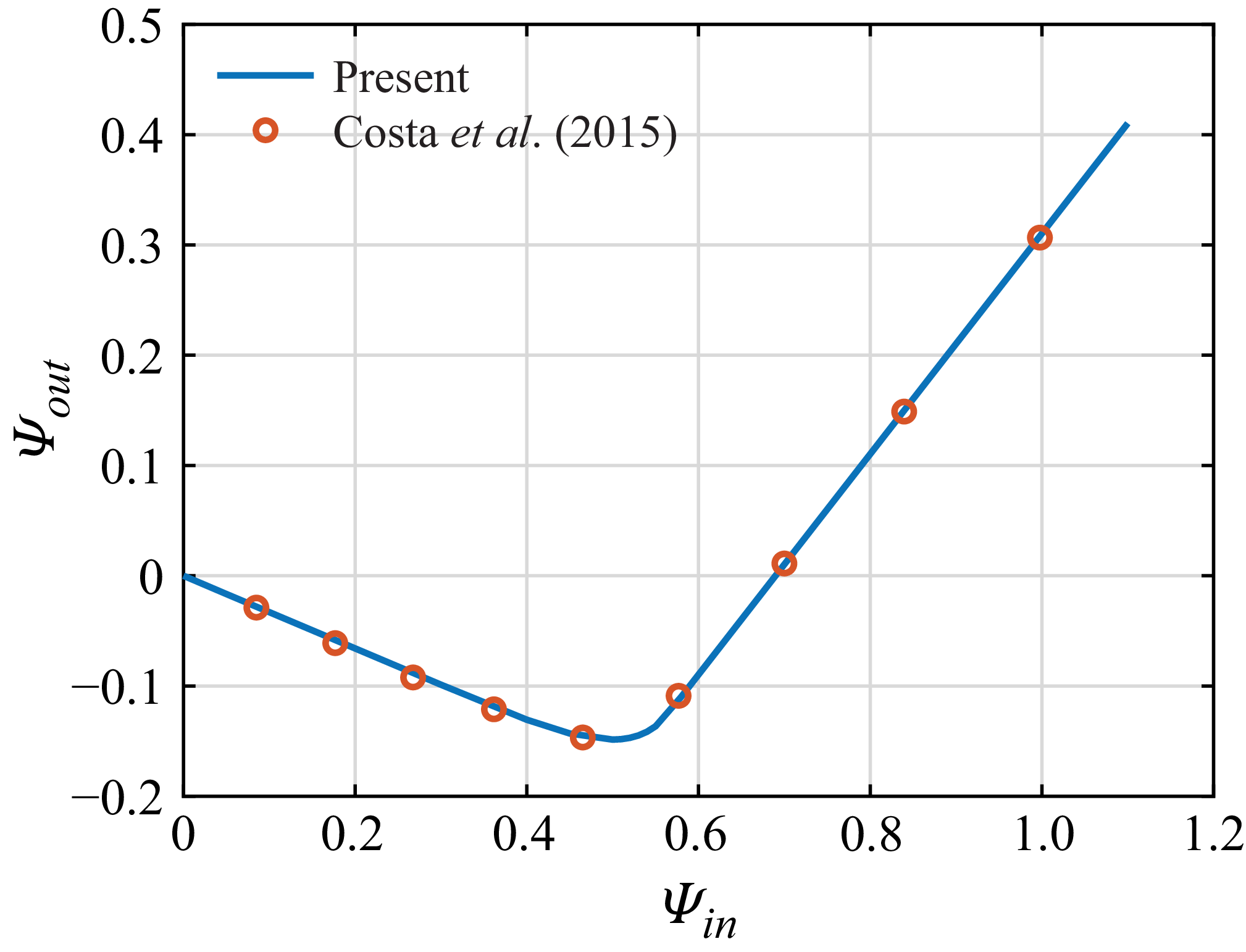
This appendix presents the validation of the point-particle solver, where each interaction model component is validated individually. Specifically, the first case validates the cohesive force model and the normal component of the lubrication force. The second case focuses on validating the tangential component of the lubrication force and the lubrication torque. The third case validates the collision force and torque.
The first case considers particles in a Taylor–Green vortex flow, described by the velocity components
 \begin{equation} u_{\!f} =\frac {U}{\pi } \sin \left (\frac {\pi x}{L}\right ) \cos \left (\frac {\pi y}{L}\right ), \quad v_{\!f} =-\frac {U}{\pi } \cos \left (\frac {\pi x}{L}\right ) \sin \left (\frac {\pi y}{L}\right ), \end{equation}
where
 $L$
and
 $U$
represent the characteristic length and velocity scales of the vortex flow. Two particles are positioned symmetrically to the left and right of the stagnation point at
 $(1,1)$
, with initial positions at
 $(0.94875, 1.0)$
and
 $(1.05125, 1.0)$
, respectively. These positions correspond to a surface distance where the cohesive force reaches its maximum. The particle parameters are
 $D_{\!p} = 0.1$
,
 $\rho _s = 1$
,
 ${\textit{St}} = 0.1$
, where the Stokes number is
 ${\textit{St}}=U\rho _sD^2_{\! p}/(18L\nu )$
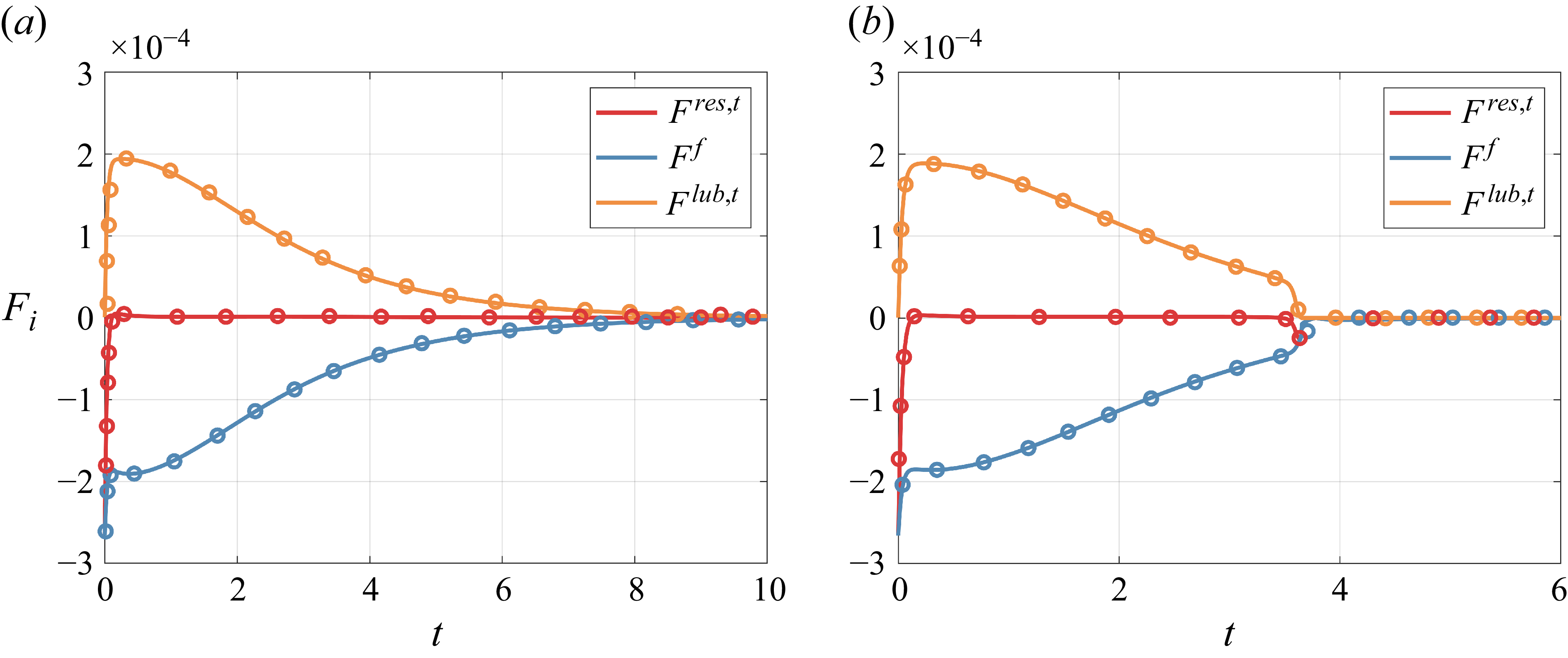
. Readers can refer to Zhao et al. (Reference Zhao, Vowinckel, Hsu, Köllner, Bai and Meiburg2020) for more details on the case set-up. Figure 15 presents the temporal evolution of the various forces acting on the particle to the left of the stagnation point. It can be observed that the present results align perfectly with the reference results from Zhao et al. (Reference Zhao, Vowinckel, Hsu, Köllner, Bai and Meiburg2020), thereby validating the cohesive force model and the normal component of the lubrication force within the particle solver.
Transient forces on the particle to the left of the stagnation point during binary interaction. The simulation parameters are
 $D_{\! p}=0.1$
,
 $\rho _s=1$
and
 ${\textit{St}}=0.1$
, for: (a) aggregation,
 ${\textit{Co}}=1\times 10^{-3}$
; (b) breakage,
 ${\textit{Co}}=2\times 10^{-4}$
. The reference results, denoted by circles, are from Zhao et al. (Reference Zhao, Vowinckel, Hsu, Köllner, Bai and Meiburg2020). The line represents the calculated results.

Transient tangential forces acting on particle
 $p$
during binary interaction. The simulation parameters are
 $D_{\! p}=0.1$
,
 $\rho _s=1$
and
 ${\textit{St}}=0.1$
, for: (a) aggregation,
 ${\textit{Co}}=4\times 10^{-4}$
; (b) breakage,
 ${\textit{Co}}=2\times 10^{-4}$
. The circles represent the reference results from private communication with Zhao K. The line represents the calculated results. The normal vector is directed from particle
 $p$
to particle
 $q$
, and the tangential vector is obtained by rotating the normal vector
 $90 ^\circ$
anticlockwise.

The second case also considers particles in the Taylor–Green vortex flow described by (A1). The two particles are initially positioned at
 $(1.0-0.05125\sqrt {2}/2, 1.0+0.05125\sqrt {2}/2)$
and
 $(1.0+0.05125\sqrt {2}/2, 1.0-0.05125\sqrt {2}/2)$
, denoted as
 $p$
and
 $q$
, respectively. The particle parameters are
 $D_{\!p} = 0.1$
,
 $\rho _s = 1$
,
 ${\textit{St}} = 0.1$
. Figure 16 presents the temporal evolution of the various forces acting on particle
 $p$
. It can be seen that the present results are in perfect agreement with the reference results, confirming the accuracy of the tangential component of the lubrication force and the lubrication torque within the particle solver.
Normalised incidence and rebound angles obtained from oblique particle–wall collisions in a dry system. The red circles represent results from Costa et al. (Reference Costa, Boersma, Westerweel and Breugem2015), while the line represents the present calculated results.

Finally, to validate our implementation of the collision force and torque model, we consider an oblique particle–wall collision in a dry system. The collisional properties of the particles, along with other physical parameters used in the simulations, are consistent with those in Costa et al. (Reference Costa, Boersma, Westerweel and Breugem2015). The effective angles of incidence and rebound are defined as
 \begin{equation} \varPsi _{\textit{in}}=\frac {u_{\textit{in}, t}}{u_{\textit{in}, n}}, \quad \varPsi _{\textit{out}}=\frac {u_{\textit{out}, t}}{u_{\textit{in}, n}}, \end{equation}
where
 $u_{\textit{in}, n}$
,
 $u_{\textit{in}, t}$
,
 $u_{\textit{out}, n}$
and
 $u_{\textit{out}, t}$
are the normal and tangential components of the incident and rebound velocities, respectively. Figure 17 compares the normalised incidence and rebound angles obtained from oblique collisions for steel spheres. The simulations show excellent agreement with the reference data from Costa et al. (Reference Costa, Boersma, Westerweel and Breugem2015) across the full range of incidence angles, thereby validating the collision force and torque model.
Appendix B. Elastic deformation and choice of cohesive model
The cohesive contact between elastic spheres can be described within two classical theoretical frameworks. The first is the DMT model (Derjaguin et al. Reference Derjaguin, Muller and Toporov1975), in which the cohesive and elastic forces are treated as additive because particle deformation during contact is negligible. The second is the Johnson–Kendall–Roberts (JKR) model (Johnson, Kendall & Roberts Reference Johnson, Kendall and Roberts1971), which accounts for significant elastic flattening at the contact area, leading to the cohesive forces scaling with the contact area. The applicability of either framework is typically assessed using the dimensionless Tabor parameter
 $\mu _T$
, which quantifies the relative importance of elastic deformation compared to the range of surface forces (Tabor Reference Tabor1977):
 \begin{equation} \mu _T=\left ( \frac { R_{ij}\left (\Delta \gamma \right )^2}{E^{*2}z_0^3} \right )^{1/3}. \end{equation}
Here,
 $R_{ij}=D_p/4$
is the reduced radius,
 $\Delta \gamma$
is the work of adhesion, and
 $E^*=E/(2-2\nu _T^2)$
is the combined elastic modulus of the two spheres with elastic modulus
 $E$
and Poisson ratio
 $\nu _T$
. The equilibrium separation distance is estimated as
 $z_0 = (9\pi \gamma R_{ij}^2/E)^{1/3}$
(Chen et al. Reference Chen, Li and Marshall2019), and the surface energy is given by
 $\gamma =A_H/(24\pi \delta ^2)$
, with characteristic length
 $\delta =0.165\ \textrm {nm}$
(Marshall & Li Reference Marshall and Li2014; Yao & Capecelatro Reference Yao and Capecelatro2021).
In the present simulations, the particle diameter is fixed at
 $D_p=5\ {\unicode{x03BC}} \textrm{m}$
, while the Hamaker constant
 $A_H$
ranges from
 $2.0\times 10^{-20} \, \textrm {J}$
to
 $2.74\times 10^{-19} \, \textrm {J}$
, corresponding to surface energies between
 $0.012 \ {\textrm{J}\ \textrm{m}^{-2}}$
and
 $0.134 \ {\textrm {J}\ \textrm{m}^{-2}}$
. Under these conditions, the estimated Tabor parameter remains below 0.03 for natural sediment materials (table 3). Even when the elastic modulus and Poisson ratio vary widely (
 $E \gt 0.1$
GPa and
 $0 \lt \nu _T \lt 1$
), the resulting
 $\mu _T$
values stay below 0.1 due to the small contact radius and adhesion energy. According to the Johnson–Greenwood transition mapping (Johnson & Greenwood Reference Johnson and Greenwood1997), the pull-off force varies smoothly from the DMT prediction for
 $\mu _T \lt 0.1$
to the JKR prediction for
 $\mu _T\gt 5$
. Therefore, the conditions considered in this study clearly fall within the DMT regime, justifying the assumption that cohesive and collision forces can be treated as additive.
Representative values of the Tabor parameter
 $\mu _T$
for natural sediments with particle diameter
 $D_p = 5\,{\unicode{x03BC}} \textrm{m}$
and surface energies in the range
 $\gamma = 0.012 {-} 0.047\ {\textrm {J}\ \rm m^{-2}}$
. The corresponding elastic and Poisson parameters are from Hamilton (Reference Hamilton1971).

Appendix C. Effect of collision time scale on the results
To validate the usage of a linear spring model, a few simulations were performed with different temporal resolutions
 $N\Delta t$
for resolving particle collisions. Figure 18 shows essentially identical results concerning the temporal evolution of the floc number
 $N_{\!f}$
and the PDFs of floc lifetime. This confirms that the time scale associated with collision physics, which is much smaller than the particle–fluid interactions, has a negligible effect on the flocculation dynamics in the present study. Based on these tests,
 $N=2$
is selected for all simulations.
Results for different time spans
 $N\Delta t$
used to resolve the particle collisions: (a) temporal evolution of the number of flocs
 $N_{\!f}$
; (b) PDFs of floc lifetime. The Reynolds number is
 ${\textit{Re}}_\lambda =35$
, the cohesive number is
 ${\textit{Co}}=3.2\times {10}^{-7}$
, and the Stokes number is
 ${St}_\eta =1$
.