2 Experimental procedure

Measurements were performed in the University of Southampton’s suction wind tunnel. The working section of this tunnel is 0.9 m  $\times$  0.6 m  $\times$  4.5 m. Free-stream turbulence was generated by a $11\times 7$ active grid placed at the inlet of the working section. The use of an active grid was inspired by Sharp et al. (Reference Sharp, Neuscamman and Warhaft2009) who used a similar set-up. The active grid is composed of 55.9 mm  $\times$  55.9 mm square wings mounted to round rods that are actuated by stepper motors in the style of Makita (Reference Makita1991). 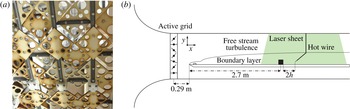The square wings have round holes that remove 25 % of the square’s surface area (figure 1 a); see Dogan et al. (Reference Dogan, Hanson and Ganapathisubramani2016) for more details on the active grid. The boundary layer was formed on an artificial floor beginning 0.29 m downstream of the grid. A trailing edge flap and the height of the artificial floor were used to position the stagnation point on the tip of the leading edge of the artificial floor and to create an approximately zero pressure gradient. A ‘zig-zag’ roughness strip, located just downstream of the leading edge, was used to trip the boundary layer. For each test, the centre of the cube was located 2.7 m downstream from the leading edge of the artificial floor. A schematic of the set-up is provided in figure 1(b).

Figure 1.

Experimental design: (a) active grid wings and (b) schematic of measurement apparatus.

Four test cases with increasing free-stream turbulence intensity ( $u_{\infty }^{\prime }/U_{\infty }$ ) were investigated for constant $h/\unicode[STIX]{x1D6FF}\approx 0.47$ and $Re_{x}\approx 1.83\times 10^{6}$ ( $U_{\infty }\approx 10~\text{m}~\text{s}^{-1}$ ). One of the primary effects of FST on a TBL for constant $Re_{x}$ is that $\unicode[STIX]{x1D6FF}$ grows (table 1). As such, the size of the cube was varied with $u_{\infty }^{\prime }/U_{\infty }$ in order to keep $h/\unicode[STIX]{x1D6FF}$ approximately constant. The size of each cube is provided in table 1 along with $\unicode[STIX]{x1D6FF}$ , which was estimated as $\unicode[STIX]{x1D6FF}_{0.99}$ from the region at least $3h$ upstream of the cube. The values of $h/\unicode[STIX]{x1D6FF}$ and $Re_{x}$ for each case are also provided in table 1 along with the Reynolds numbers based on the velocity at the cube height, $Re_{h}=U_{h}h/\unicode[STIX]{x1D708}$ , and the momentum thickness, $Re_{\unicode[STIX]{x1D703}}=U_{\infty }\unicode[STIX]{x1D703}/\unicode[STIX]{x1D708}$ , for comparison to other studies. Castro & Robins (Reference Castro and Robins1977) found that there were no discernible Reynolds number effects for turbulent incoming conditions if $Re_{h}>4000$ and the present measurements exceed this $Re_{h}$ by an order of magnitude. Additionally, we have used a trip that is most like that which produced the ‘standard’ canonical results in Marusic et al. (Reference Marusic, Chauhan, Kulandaivelu and Hutchins2015), and $Re_{\unicode[STIX]{x1D703}}>2000$ for all cases which is within the range where the influence of the tripping conditions are negligible according to Schlatter & Örlü (Reference Schlatter and Örlü2012).

Table 1.

Free-stream and incoming flow conditions for all test cases. Free-stream turbulence statistics were measured by the hot-wire probe at $y=212$  mm, which is ${>}2\unicode[STIX]{x1D6FF}$ for all cases. The boundary layer thickness, $\unicode[STIX]{x1D6FF}=\unicode[STIX]{x1D6FF}_{0.99}$ , and the turbulent statistics at the cube height were measured with PIV. The incoming $\unicode[STIX]{x1D6FF}$ and $L_{u}$ were assessed at least $3h$ upstream of the cube.

The four tests of table 1 have increasing free-stream turbulence intensity: $u_{\infty }^{\prime }/U_{\infty }=0.5\,\%$ , 3.7 %, 7.1 % and 8.9 %. The lowest turbulence intensity case, A, represents a canonical TBL with approximately no FST. This flow was generated without the active grid and is typically excluded from comparison to the other cases because its shear and velocity profile differ significantly from the others. However, it is presented as a canonical baseline. The $u_{\infty }^{\prime }/U_{\infty }=3.7\,\%$ case, B, was generated with the active grid in place, but held in a static position with half the wings perpendicular to the mean flow direction and the other half parallel to the mean flow direction, in an alternating pattern. The two higher turbulence intensity cases, C and D, were generated with the active grid operating in the ‘fully random’ mode described by Hearst & Lavoie (Reference Hearst and Lavoie2015) with each motor receiving its own random top-hat distribution of time between updating motor commands (0.05 s ${\leqslant}t\leqslant 2.5$  s), wing acceleration (50 Hz/s ${\leqslant}\unicode[STIX]{x1D6FC}\leqslant 200~\text{Hz}~\text{s}^{-1}$ ) and wing velocity ( $5~\text{Hz}\leqslant \unicode[STIX]{x1D714}\leqslant 15~\text{Hz}$ for case C, and $1~\text{Hz}\leqslant \unicode[STIX]{x1D714}\leqslant 3~\text{Hz}$ for case D).

For the PIV measurements, the flow was seeded with smoke droplets (diameter ${\sim}1~\unicode[STIX]{x03BC}\text{m}$ ). Two pulsed Litron Nd-YAG lasers (532 nm, 200 mJ) were used simultaneously to create an extended laser sheet in the streamwise/wall-normal plane along the cube’s axis of symmetry (centreline). Three adjacent LaVision ImagerProLX 16 mega-pixel cameras equipped with Sigma DG 105 mm lenses were oriented along the streamwise direction to capture the upstream flow and the wake of the cube. The resulting field-of-view (FOV) was 200 mm high, and 700 mm long. Vector fields were computed with DaVis 8.2.2 on graphical processing units using multiple passes beginning with a coarse grid (64 pixels  $\times$  64 pixels) and refined to a fine grid (24 pixels  $\times$  24 pixels). Using an overlap of 50 %, the distance between two adjacent vectors is approximately 0.7 mm. The characteristic dimension of the cube, $h$ , is described by a minimum of 28 vectors for the worst case. Two thousand image pairs were acquired at an acquisition frequency of 0.25 Hz, which resulted in all vector fields representing independent samples.

Hot-wire anemometry measurements were performed with an automated traverse and a Dantec StreamLine constant temperature anemometer. A single-wire probe (5  $\unicode[STIX]{x03BC}\text{m}$ diameter tungsten wire; 1 mm sensing length), made in-house and mounted to Dantec-style prongs, was used to perform the measurements. The wire was calibrated in situ using a 12 point variable exponent King’s Law. Data were acquired for 7 min at a sampling frequency of $f_{s}=70.2$  kHz with an analogue filter set at $f_{c}=30.0$  kHz. This resulted in a minimum of 40 000 boundary layer turn overs, which is ample data to converge the spectra and second-order statistics in both the free stream and the boundary layer. Hot-wire measurements were performed at five wall-normal locations $2h$ downstream of the cube: $y/h=0.75$ , 1.0, 1.5, 2.0 and at a fixed free-stream position ( $y=212$  mm), which is approximately equidistant from the top wall and the artificial floor, and greater than $2\unicode[STIX]{x1D6FF}$ in all cases. The post-processing used here is described in detail by Hearst & Lavoie (Reference Hearst and Lavoie2014). Gradient quantities were estimated from the hot-wire data using a sixth-order centred-difference scheme, which offers a good balance between accuracy and high-frequency filtering for hot-wire measurements (Hearst et al. Reference Hearst, Buxton, Ganapathisubramani and Lavoie2012).

Figure 2.

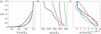
Profiles of the incoming turbulent flow: (a) incoming mean velocity, (b) incoming turbulence intensity and (c) incoming Reynolds shear stress. Cases: (♢) A, (▫) B, (○) C and (▵) D.

3 Incoming flow conditions

The incoming mean velocity ( $U_{i}$ ), turbulent fluctuations ( $u_{i}^{\prime }$ ) and Reynolds shear stress ( $u^{\prime }v_{i}^{\prime }$ ) profiles measured with PIV are given for each case in figures 2(a), 2(b) and 2(c), respectively (subscript $\cdot _{i}$ denotes incoming conditions). As $u_{\infty }^{\prime }/U_{\infty }$ was increased, $\unicode[STIX]{x1D6FF}$ increased (table 1) and the boundary layer became fuller. In addition, as the FST was increased, the turbulence intensity profile had less variation and a higher turbulence intensity was achieved closer to the wall (figure 2 b). Figure 2(c) shows that the greatest magnitude Reynolds shear stress at the cube height occurred for the canonical case, and that it monotonically decreased with increasing $u_{\infty }^{\prime }/U_{\infty }$ . The changes in $u^{\prime }v_{i}^{\prime }$ between cases are marginal and the effect of them on the wakes is investigated in the subsequent section. The difference in the profile for case B is likely related to the high static blockage of the unactuated grid. However, as will be shown, $u^{\prime }v_{i}^{\prime }$ does not have a significant impact on the wake flow. For the three test cases with added FST (B, C, D), the relative velocity and mean shear at the cube height changed marginally, $0.92\leqslant U_{h}/U_{\infty }\leqslant 0.94$ and $0.09\leqslant \hat{\unicode[STIX]{x1D70F}}_{h}\leqslant 0.11$ , respectively (table 1). Furthermore, the non-dimensional momentum in the mean profile beneath the cube height, $\int _{0}^{1}(U/U_{\infty })\,\text{d}(y/h)$ , was between 7.6 and 7.9 for cases B, C and D, compared to 6.7 for case A. The FST cases experienced an increase in local turbulence intensity of $6.3\,\%\leqslant u_{h}^{\prime }/U_{h}\leqslant 9.0\,\%$ with increasing $u_{\infty }^{\prime }/U_{\infty }$ (table 1). Thus, there are three cases (B, C, D) with roughly $U_{h}/U_{\infty }\approx 0.93$ , $\hat{\unicode[STIX]{x1D70F}}_{h}\approx 0.1$ and a similar degree of incoming momentum, but a range of $u_{h}^{\prime }/U_{h}$ , allowing us to comment on the effect of $u_{h}^{\prime }/U_{h}$ independently of mean velocity profile characteristics. In contrast, case A has a normalised shear level that is a factor of 2 different from the FST cases and as such it is not directly included in the turbulence intensity comparison.

Table 1 also includes estimates of the incoming integral length scale at the cube height ( $L_{h}$ ) estimated from PIV at least $3h$ upstream of the cube. Here, $L$ is estimated by integrating the autocorrelation to the first zero-crossing. The zero-crossings of the correlations were similar to those reported by Ganapathisubramani et al. (Reference Ganapathisubramani, Hutchins, Hambleton, Longmire and Marusic2005). Despite the jump to higher $L_{h}/h$ for cases A and B relative to C and D, $L_{h}/h\leqslant 0.4$ for all cases, which is within the range that previous studies observed no significant effect of $L$ (Hillier & Cherry Reference Hillier and Cherry1981; Li et al. Reference Li, Hu and Yan2014).

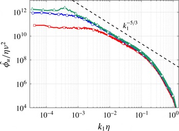
Figure 3 shows the one-dimensional velocity spectra in wavenumber space, $\hat{\unicode[STIX]{x1D719}}_{u}(k_{1})$ , normalised by Kolmogorov variables for the three FST cases; $\unicode[STIX]{x1D702}=\unicode[STIX]{x1D708}^{3/4}/\langle \unicode[STIX]{x1D716}\rangle ^{1/4}$ is the Kolmogorov microscale where $\langle \unicode[STIX]{x1D716}\rangle =15\unicode[STIX]{x1D708}\langle (\unicode[STIX]{x2202}u/\unicode[STIX]{x2202}x)^{2}\rangle$ is the dissipation rate of turbulent kinetic energy assuming isotropy. For the hot-wire, Taylor’s frozen flow hypothesis was employed, that is $(\unicode[STIX]{x2202}/\unicode[STIX]{x2202}t)=U(\unicode[STIX]{x2202}/\unicode[STIX]{x2202}x)$ . The velocity wavenumber spectra show a near, but not exact, $k_{1}^{-5/3}$ range for the FST cases that spans a larger wavenumber space and better approximates $k_{1}^{-5/3}$ as $Re_{\unicode[STIX]{x1D706},\infty }=u_{\infty }^{\prime }\unicode[STIX]{x1D706}_{\infty }/\unicode[STIX]{x1D708}$ is increased, where $\unicode[STIX]{x1D706}^{2}=\langle u^{2}\rangle /\langle (\unicode[STIX]{x2202}u/\unicode[STIX]{x2202}x)^{2}\rangle$ is the square of the Taylor microscale. This result is in agreement with previous active grid studies (Mydlarski & Warhaft Reference Mydlarski and Warhaft1996; Hearst & Lavoie Reference Hearst and Lavoie2015), and validates that there is a fully developed turbulent free stream above the TBL.

Figure 3.

Kolmogorov variable normalised free-stream wavenumber spectra for turbulent cases: (▫) B, (○) C and (▵) D.

Figure 4.

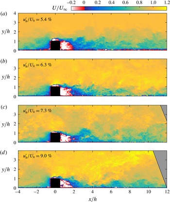
Sample instantaneous streamwise velocity fields for each test case.

4 Spatial characteristics of the wake

Representative instantaneous streamwise velocity fields from the PIV measurements are shown in figure 4. This figure provides the first insight into the flow phenomenology, and the differences and similarities between cases. A similarity between all three cases is that the flow appears to be attached to the top surface, at least near the trailing edge. Key indicators of this are the positive streamwise velocity after the negative separation bubble on the top surface of the cube, and the lack of a distinct shear layer leaving the downstream top edge of the cube. Also visible is the difference in the incoming flow field between the cases. In particular, the canonical case differs in that there is a larger momentum deficit upstream of the cube instantaneously than the more turbulent cases, which is supported by the profiles provided in figure 2. Lastly, in the wakes, the deficit region appears to be closer to the cube for increasing $u_{h}^{\prime }/U_{h}$ . It thus seems relevant to both consider the mean velocity fields as well as compare the statistics of the flow fields with the incoming profile removed in order to ascertain how rapidly the flow returns to its upstream state. Furthermore, with respect to the attachment of the flow to the top surface, statistics are required to adequately interpret the flow state on the top surface of the cube.

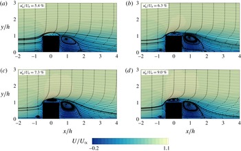
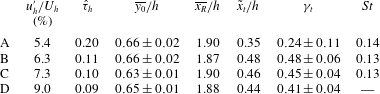
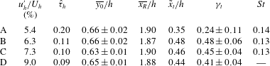
The mean flow field obtained from the PIV measurements is shown for each case in figure 5, where mean streamlines are superimposed on the mean streamwise velocity fields. In general, the flow structure in the immediate proximity of the cube is not strongly dependent on the incoming flow conditions investigated here. From the mean streamline figures, a stagnation point ( $y_{0}$ ) on the front face of the cube was observed at an approximate mean height $\overline{y_{0}}/h\approx 0.65$ for all cases (within uncertainty), and thus did not show a strong dependence on either $u_{h}^{\prime }/U_{h}$ or $\hat{\unicode[STIX]{x1D70F}}_{h}$ (table 2). Downstream of the cube, the flow was characterised by a recirculation region. The mean reattachment point of this region was estimated from the streamline plot, and was $\overline{x_{R}}/h=1.9$ for all cases (table 2), which is also independent of $u_{h}^{\prime }/U_{h}$ and $\hat{\unicode[STIX]{x1D70F}}_{h}$ ; this is $1.4h$ downstream of the rear face of the cube. This location is consistent with that observed in the wake of a cube in channel flow (Hussein & Martinuzzi Reference Hussein and Martinuzzi1996), and the relative independence of its position with changing turbulence intensity is supported by the measurements of Ballio et al. (Reference Ballio, Bettoni and Franzetti1998).

Figure 5.

Mean streamwise velocity fields for each case with superimposed mean streamlines.

Above the cube, a recirculation bubble forms due to the separating shear layer at the leading edge. The separated flow attaches to the top surface of the cube intermittently. The ‘reattachment’ of the shear layers formed on a cube was previously observed for cubes immersed in a turbulent flow (Castro & Robins Reference Castro and Robins1977; Meinders et al. Reference Meinders, Hanjalic and Martinuzzi1999), although we use the terminology ‘attach’ to the top surface to distinguish this phenomenon from that in the wake and because the flow was not initially attached to the top surface. The intermittency of attachment to the top surface is one of the first signs of the effects of varying the incoming conditions. The intermittency for each case is provided in table 2 with uncertainty estimates that vary with the resolution ( $\unicode[STIX]{x1D6FE}_{t}=0$ implies the flow always attaches to the top surface). For cases B, C and D at the same $\hat{\unicode[STIX]{x1D70F}}_{h}\approx 0.1$ , the flow more frequently attaches to the top surface, and thus the intermittency decreases, with increasing $u_{h}^{\prime }/U_{h}$ . This corresponds to the median point of attachment to the top surface ( $\tilde{x}_{t}/h$ ), which approaches the leading edge of the cube as the intermittency drops and $u_{h}^{\prime }/U_{h}$ increases. This agrees with observations of the separation and attachment on a thick flat plate subjected to FST (Saathoff & Melbourne Reference Saathoff and Melbourne1997). We attribute the significant differences in intermittency between the canonical case A, and the FST cases to the difference in $\hat{\unicode[STIX]{x1D70F}}_{h}$ .

The same technique as Pearson, Goulart & Ganapathisubramani (Reference Pearson, Goulart and Ganapathisubramani2013) was employed to determine the reattachment location in the wake of the cube, as well as the attachment location and intermittency on the top surface. Our particular application of this technique was to look for the first position where instantaneously $U<0$ against the boundary while scanning from a downstream position towards an upstream position. This is similar to how mean recirculation was determined in previous studies with hot-wires or tufts (Antoniou & Bergeles Reference Antoniou and Bergeles1988). The intermittency was inferred from assessing the percentage of samples in which an attachment point was found on top of the cube.

Table 2.

Characteristics of the flow in the immediate proximity of the wall-mounted cubes. The uncertainties in position are the same for $\overline{y_{0}}/h$ , $\overline{x_{R}}/h$ and $\tilde{x}_{t}/h$ .

Upstream of the cubes, a horseshoe vortex forms. The centre location of the horseshoe vortex also appears to show some dependence on the incoming conditions. For canonical case A, the horseshoe vortex is centred near $(x/h,y/h)=(-0.8,0.04)$ , while for the three FST cases it is centred near $(x/h,y/h)=(-0.8,0.1)$ . The latter is similar to the horseshoe vortex core location reported by Lim, Thomas & Castro (Reference Lim, Thomas and Castro2009) for LES of a TBL immersed cube. Furthermore, for turbulent incoming conditions, Baker (Reference Baker1980) found that the centre of the horseshoe vortex occurred near $x/h=-0.8$ and that its position was independent of Reynolds number. The rising of the horseshoe vortex core away from the wall for increased turbulence was also observed by Vinuesa et al. (Reference Vinuesa, Schlatter, Malm, Mavriplis and Henningson2015) in their DNS comparing incoming Blasius profile boundary layers to canonical TBLs interacting with the lower part of a square cylinder. However, we note that for our three cases with approximately constant $\hat{\unicode[STIX]{x1D70F}}_{h}$ , but increasing $u_{h}^{\prime }/U_{h}$ , the core does not appreciable change location, suggesting its movement is linked to mean shear rather than turbulence intensity.

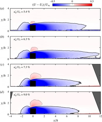
Figure 6 shows the streamwise velocity field with the incoming profile (figure 2) removed for all cases. Contours at $|(U-U_{i})/U_{\infty }|=0.05$ are included in figure 6. This threshold was chosen as a relative indicator of mean wake length, and in general the conclusions are not sensitive to the choice of threshold. It was also chosen to be at approximately $u_{h}^{\prime }/U_{h}$ of the lowest turbulence intensity case (case A). First, consider the three cases at the same normalised shear $\hat{\unicode[STIX]{x1D70F}}_{h}\approx 0.1$ (B, C, D). The two higher $u_{h}^{\prime }/U_{h}$ cases (C and D) both have a smaller deficit region upstream of them relative to case B. Downstream of the cube, the longest wake (with respect to the mean streamwise velocity deficit) occurs for case B. For B, the $-0.05$ contour level extends to a maximum streamwise location of $x/h=11.8$ compared to 8.6 for C and 8.2 for D. This illustrates a monotonic reduction in the wake length relative to case B of 27 % and 31 % for cases C and D, respectively, at fixed $\hat{\unicode[STIX]{x1D70F}}_{h}\approx 0.1$ . These are substantial changes given the turbulence was only increased by 1 % between case B and C and 2.7 % between B and D. This wake reduction also corresponds to a reduction in $\unicode[STIX]{x1D6FE}_{t}$ with $u_{h}^{\prime }/U_{h}$ .

Figure 6.

Mean streamwise velocity field with the incoming profile removed. Contour lines at: (dashed)  $+0.05$ and (solid)  $-0.05$ .

The difference between cases B and C is markedly more substantial than that between cases C and D. This may suggest that the ability of the turbulent fluctuations to facilitate wake recovery saturates beyond a certain turbulence intensity. There are at least two possible causes of this. First, it is possible that there is a balance between the turbulence level at the height of the obstacle and the turbulence generated by the obstacle in its wake. Therefore, beyond a certain level it might not be possible to alter the entrainment in the wake any further, resulting in a system of diminishing returns as $u_{h}^{\prime }/U_{h}$ is increased. Alternatively, the significant difference may be related to the size of the incoming large scales at the cube height, which is $L_{h}/h=0.34$ for case B, but $L_{h}/h\approx 0.19$ for cases C and D. While these are all below the threshold for which no significant effects were noted for the separation bubbles and drag forces in previous studies (Saathoff & Melbourne Reference Saathoff and Melbourne1997; Li et al. Reference Li, Hu and Yan2014), it is possible that the 1.5 times larger large scales for case B relative to cases C and D results in less frequent transport of high-speed fluid into the wake relative to $h$ . Regardless, of the above, the results are significant in that they show a monotonic decrease in the mean wake deficit region with increasing $u_{h}^{\prime }/U_{h}$ .

Figure 7.

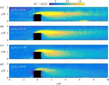
Streamwise velocity fluctuations compared to the incoming velocity fluctuation profile.

In figure 6, the canonical case A has a shorter wake than B. This is attributable to the significant difference between $U_{h}/U_{\infty }$ and $\hat{\unicode[STIX]{x1D70F}}_{h}$ for A compared to B. In particular, case B has a much fuller profile at the cube height, with $U_{h}/U_{\infty }=0.92$ , compared to $U_{h}/U_{\infty }=0.85$ . For this range, the turbulence intensity varies by less than $1\,\%$ between them. Thus, the distance required to recover the upstream velocity for case B is longer and the evidence suggests the turbulence intensity is of insufficient magnitude to facilitate wake recovery. In addition, the magnitude of $\hat{\unicode[STIX]{x1D70F}}_{h}$ for case A is nearly twice that of B, because of the shallower slope of the velocity profile at the cube height (figure 2). This also indicates that there is lower incoming momentum for case A over the characteristic dimension $h$ , and thus, for a similar amount of turbulent kinetic energy, the wake recovers to the same low flow state over less distance.

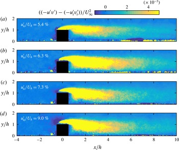
Figure 7 shows the normalised streamwise velocity fluctuation deficit relative to the incoming turbulence intensity profile. These maps allow for visualisation of the ratio of increase or decrease in the fluctuations compared to the incoming flow at each wall-normal position. Figure 7 highlights that the fluctuations recover to their original state closer to the cube for increasing $u_{h}^{\prime }/U_{h}$ , in agreement with the results for the mean velocity. These results are suggestive that the increase in turbulence intensity at the cube height facilitates the transport of high momentum fluid into the wake, thus decreasing the wake length. This is corroborated in figure 5 by the strong downward velocity after the recirculation region in the wake of the cube that deflects the streamlines downward and that likely acts to entrain faster moving fluid into the wake from above. The increased turbulence intensity below $h$ for increasing $u_{h}^{\prime }/U_{h}$ suggests a similar mechanism would move high momentum fluid laterally into the wake as well.

Maps of the mean Reynolds shear stress are provided in figure 8. The disturbance to the incoming $u^{\prime }v^{\prime }$ profile extends beyond the measurement range of the present set-up although $u^{\prime }v^{\prime }$ is clearly recovering at the end of the FOV. The wakes of the three cases at $\hat{\unicode[STIX]{x1D70F}}_{h}\approx 0.1$ do not substantially differ with respect to $u^{\prime }v^{\prime }$ , while canonical case A with $\hat{\unicode[STIX]{x1D70F}}_{h}=0.2$ has a smaller $u^{\prime }v^{\prime }$ deficit region in its wake. This suggests that the $u^{\prime }v^{\prime }$ recovery is primarily dependent on mean shear rather than turbulence intensity. Despite the marginally differing incoming $u^{\prime }v^{\prime }$ profiles highlighted in figure 2(c), the wake appears to scale with this difference if $\hat{\unicode[STIX]{x1D70F}}_{h}$ is maintained thus marginalising the importance of the incoming $u^{\prime }v^{\prime }$ profile for such cases.

Figure 8.

Mean Reynolds shear stress fields with the incoming mean Reynolds shear stress profile removed.

5 Time series in the wake

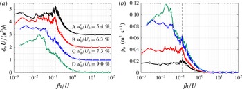
In the context of bluff bodies immersed in approximately homogeneous FST, increased turbulence intensity appeared to correlate with a reduction in the strength of vortex shedding motions (Blackburn & Melbourne Reference Blackburn and Melbourne1996; Rind & Castro Reference Rind and Castro2012). A similar phenomenon is investigated here with hot-wire anemometry measurements in the wake. The frequency domain velocity spectra, $\unicode[STIX]{x1D719}_{u}(f)$ , normalised by large-scale variables, are shown in figure 9(a) at $(x/h,y/h)=(2.5,0.75)$ for all cases; this wall-normal position was chosen to ensure the probe was completely immersed in the wake. Given that $\overline{x_{R}}/h$ is approximately fixed for all cases, the probe is in the same position relative to the primary wake circulation region. Note that the origin of the $x$ -axis is at the centre of the cube, so this position is $2h$ downstream of the rear face of the cube. In figure 9(a), a dominant non-dimensional shedding frequency is apparent for the lower turbulence intensity cases, A and B, at a local Strouhal number of $St=fh/U\approx 0.13$ . This is similar to the dominant shedding peak at $St\approx 0.1$ observed in experiments (Wang & Zhou Reference Wang and Zhou2009; Sattari, Bourgeois & Martinuzzi Reference Sattari, Bourgeois and Martinuzzi2012) and DNS (Vinuesa et al. Reference Vinuesa, Schlatter, Malm, Mavriplis and Henningson2015) of a variety of square cylinders, and $St=0.145$ observed by Hussein & Martinuzzi (Reference Hussein and Martinuzzi1996) for a cube in turbulent channel flow. This peak must be related to flow induced by the presence of the cube because there is no peak near $St=0.13$ in the incoming flow.

Figure 9.

Frequency space velocity spectra at $(x/h,y/h)=(2.5,0.75)$ for all cases: (a) normalised by large-scale variables and (b) no normalisation. Dashed line is at $St=0.13$ . Cases A, B and C are offset by $+3$ , $+2$ and $+1$ , respectively, in (a).

The shedding peak observed here has diminishing prominence and is less broadband with increasing $u_{h}^{\prime }/U_{h}$ . Here, we use the word prominence to describe the magnitude of the shedding peak relative to (or above) the energy content of the other frequencies in the normalised spectra (figure 9 a). The unnormalised wake spectra are shown in figure 9(b). From this figure it is apparent that the increased turbulence intensity results in higher energy levels at all scales $fh/U<1$ , including those surrounding the shedding frequency, thus reducing the prominence of the shedding peak relative to the background flow. This also correlates to a reduction in the intermittency of the recirculation bubble on top of the cube for the FST cases (table 2). Regardless of whether the shedding is masked or eliminated by increasing $u_{h}^{\prime }/U_{h}$ , the results suggest a suppression of the shedding motions at the $St$ prevalent in the low turbulence cases. The existence of the $St=0.13$ peak for case B and its diminishing presence for the higher cases suggests the shortening of the wake region for cases C and D is related to a reduction in the strength of the dominant shedding motions.

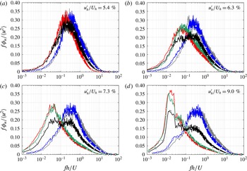
The pre-multiplied frequency spectra, $\unicode[STIX]{x1D719}_{u}(f)$ , from the $y/h$ scan are shown in figure 10 for each test case. The pre-multiplied spectrum identifies the frequencies that carry the majority of the energy in the flow. Dogan et al. (Reference Dogan, Hanson and Ganapathisubramani2016) demonstrated that the FST imposes its own shape for $\unicode[STIX]{x1D719}_{u}$ on the outer regions of the boundary layer, and this spectral shape persists until nearly $y^{+}=100$ , which is of order ${\sim}0.1\unicode[STIX]{x1D6FF}$ . This is well below $h$ in the present experiment. Thus any change to $\unicode[STIX]{x1D719}_{u}$ as one descends through the boundary layer and below $h$ must be a result of the presence of the cube.

Figure 10.

Pre-multiplied frequency spectra $2h$ downstream of the cube for all cases; (♢)  $y/h=0.75$ , (○)  $y/h=1.0$ , (▿)  $y/h=1.5$ , (▫)  $y/h=2.0$ , (▵) free-stream station.

Case D in figure 10 is a strong illustrative example of the physics at play as one enters the cube wake. The frequencies that carry the majority of the energy outside of the boundary layer are set by the FST and are identified by a peak near $fh/U=10^{-2}$ . This peak is present at $y=2h=0.92\unicode[STIX]{x1D6FF}$ and $4.4h=2\unicode[STIX]{x1D6FF}$ , and in the flows of Sharp et al. (Reference Sharp, Neuscamman and Warhaft2009) and Dogan et al. (Reference Dogan, Hanson and Ganapathisubramani2016) persisted all the way to the near-wall region. However, in the present experiment, this energy is redistributed to frequencies near $fh/U=St=0.13$ as one descends into the cube wake ( $y/h=0.75$ and 1.0). At $y/h=1.5$ , a clear transition between the two regions is apparent and the spectrum exhibits both the outer peak and the wake peak. The other three cases follow the same trend as D. That is, the FST imposes a shape and an outer peak on the spectra, but as one moves down through the boundary layer into the wake of the cube, the spectrum of the wake dominates the flow, regardless of the outer layer spectrum. The spectra in the cube wake are remarkably similar despite having transitioned from entirely different incoming conditions. This supports the observation from the present and previous studies that the downstream reattachment point is not significantly influenced by the upstream flow if it is turbulent.