Considered systems

Three different systems are considered for this study spawning a large range of complexity:

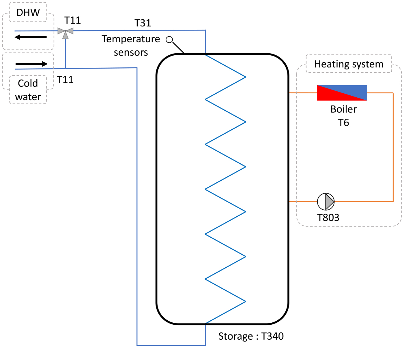
• • Configuration 1 consists of a 763 L stratified water tank connected to an electric (resistive) heating system (see Fig. 2).

• • Configuration 2 uses the same water tank powered by a heat pump (HP)

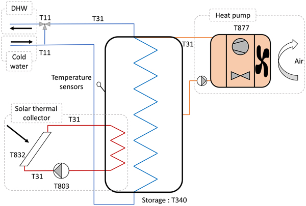
• • Configuration 3 is identical to configuration 2 with an additional solar thermal collector (STC) as an auxiliary power source (see Fig. 1).

Note that in Figures 1 and 2, Ti refers to the component of type i used in TRNSYS software.

Fig. 1.

Heat production system with solar thermal collector and heat pump.

Fig. 2.

Heat production system with electrical resistance.

Description of real consumption measurement data sets

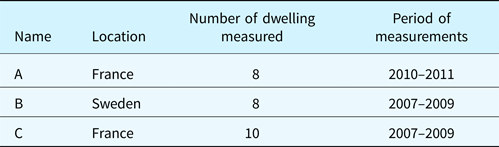
A total of 26 data sets are used to perform forecast and simulation. These real data are issued from three different locations in France and Sweden and have been gathered during the CombiSol EuropeanFootnote ⁴ and French SCHEFFFootnote ⁵ projects. The use of measurement coming from distant location ensures that the model accuracy does not depend much on the location of the dweller (and thus on their habit). These data sets will be denoted as A, B, and C, respectively, and are presented in Table 1. Each data set measures the hot water needs in liters for a real domestic dwelling. DHW consumption measurements have been performed every 6 min. Missing values generally concern <5% of the data. Linear interpolation has been performed if the time window of missing data is shorter than 3 h to complete the time series. Otherwise, the time window is not considered for the analysis.

Table 1.

List of measured dwelling grouped by project

Description of the simulation setup

All the three TRNSYS setups are derived from the core simulation setup developed for MacSheep European project provided by Chèze et al. (Reference Chèze, Bales, Betak, Broum, Heier, Heinz and Poppi2015). This setup is the most complete and energetically efficient one. The heating system comprises an HP connected to a vertical borehole heat exchanger as well as an STC. These devices are connected to a stratified water tank through double ports or heat exchangers from which hot water is drawn for domestic use.

Since STC can provide a large part of the required DHW in summer almost for free (only a pump to flow water through the collector is required), limited energy savings are expected in this configuration. However, this kind of system is not extensively used today. Thus, a second system has been designed without STC. Except the STC, this setup is perfectly equivalent to the first one. Since these two systems are not representative of what can be found as DHW heating systems, a third system has been simulated consisting of the same water tank connected to an electric boiler. The electric heater is simulated thanks to type 6 unit of TRNSYS with a maximum heating rate of 8000 kJ/h and a perfect efficiency. Although this efficiency is not relevant, it does not call into question conclusions since they will be based on relative savings considering the same system parameters with and without the forecast.

There are two different control strategies according to whether or not forecast is taken into account, that is, reactive and anticipative. Without forecasting, the control strategy is a traditional one, in other words the water is heated at the set point temperature (50°C in this case, as recommended by the European and US institutions) all the time. This is achieved using a thermostat with a hysteresis of ±2°C.

In the case where we account for the forecast, the available energy in the tank at time t is compared with the forecast quantity of energy that will be consumed during the next coming hour. If sufficient energy is stored, the heating system remains off or is switched on otherwise. A hysteresis controller is also added in this case with a dead band of at least the equivalent of 10 L of hot water or 10% of the required energy for the next hour.

Description of the forecast algorithm

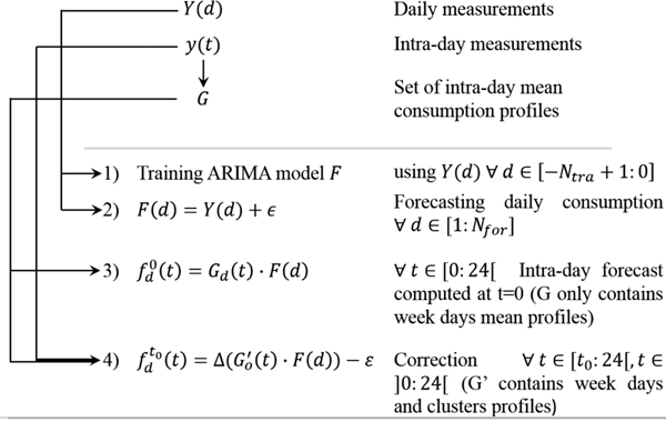
The detail of the algorithm can be found in Lomet et al. (Reference Lomet, Suard and Chèze2015). However, we briefly describe it here for convenience. The procedure is broken down into four steps that are illustrated in Figure 3 where Y(d) and F(d) are the measured and forecast daily consumption, respectively, y(t) and f(t) are the measured and forecast intra-day consumption profiles, respectively. d is the day index and t is the time index within a day (in hours), G is the pool of mean intra-day consumption profiles, N _tra and N _for are the number of days used for training and forecasting time series, respectively.

Fig. 3.

Algorithm scheme.

ARIMA modeling of daily consumption

To forecast DHW consumption, the algorithm only needs the record of the 3 last months of consumption ($Y_{\rm d}{\rm \;} \forall \; d\in {\rm \;} \lsqb {-N_{{\rm tra}} + 1:0} \rsqb $ in Fig. 3). The input for the self-learning process is thus a discrete time series of consumption in liters. The total consumption per day is modeled using an ARIMA function (Box et al., Reference Box, Jenkins and Reinsel2013). A training window of N _tra = 84 days is used to estimate the values of coefficients during the learning stage. This is the step 1 in Figure 3. Forecast is performed over a period of 1 year that follows the training window. The formula is shown in Eqs (1) and (2).

(1)$$X_{\rm t} = \mathop \sum \limits_i {\rm \varphi} _i{\rm X}_{{\rm t}-i} + \mathop \sum \limits_i \theta _i\varepsilon _{{\rm t}-i} + \varepsilon _{\rm t}\comma \,$$

(2)$$\forall \; t\in {\rm \;\ {\opf Z} }\comma \,{\rm \;} {\rm X}_{\rm t} = \nabla ^{\rm d}Y_{\rm t}\comma \,$$

where Y _t is the forecast, the parameters φ_i and θ _i are the linear coefficients, ε _t is the white noise, i ∈ {1, 2, 7}, and d is the degree of differencing. This auto regressive part is formed by a linear combination of the consumption of the two preceding days and the same day of the previous week (denoted by i ∈ {1, 2, 7}). The moving average part is also based on the error made on these days. This form of the model is fixed for all dwellings. This allows faster computation for model training, which is a great asset for embedding into the water tank. This form has been chosen so that it fits best the 26 dwellings. However, the differentiation degree is calculated independently for each dwelling in order to build the model on a stationary time series. This is the second step in Figure 3.

Intra-day consumption modeling

After forecasting the daily consumption, intra-day cumulative consumption is forecast. The method consists in building a set of normalized and representative daily load curves. Then the cumulative consumption within each day is assumed to conform to the most appropriate load curve picked from the curve set. For each day, the final forecast is obtained by scaling the normalized curve with the ARIMA forecast.

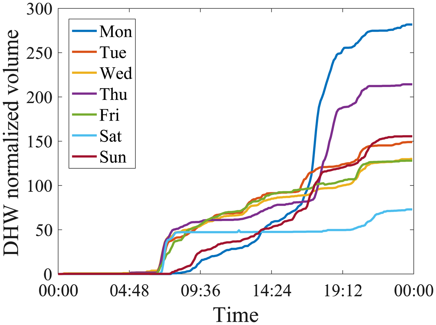
A first set of curves is built based on the day of the week. That is, each and every load curve of the same day of the week measured during the training test is gathered. The representative curve is then obtained by computing the average of the curves. This is the third step in Figure 3. As an example, intra-day profiles for dwelling A1 are plotted in Figure 4.

Fig. 4.

Intra-day DHW consumption profile of dwelling A1 for each day of the week.

Each average curve is then modeled using a sum of sigmoid functions. It enables having smoother profiles and requires less memory for embedding. Combining ARIMA forecast with the corresponding week day average cumulative consumption yields a first continuous forecast for the entire year. This is the fourth step in Figure 3.

Performance comparison protocol

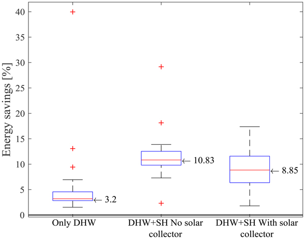
To compare the performance yield by each experiment, the energy savings after 1 year of consumption are calculated. Energy savings are the difference of the electrical energy consumed by the system that accounts for the forecast (anticipative system) and the one that does not (reactive system, which is considered as the baseline). Further results (Figs. 5, 6, 10 and 11) are shown in relative scale. These relative energy savings are computed using the formula shown in Eq. (3), where E _s is the energy saved, E _r and E _a are the energy consumed by reactive and anticipative systems, respectively.

(3)$$E_{\rm s} = \displaystyle{{E_{\rm r}-E_{\rm a}} \over {E_{\rm r}}}100.$$

Fig. 5.

Relative energy savings using the perfect forecast on the 26 dwellings depending on the considered system.

In order to have a relevant comparison between experiments, the discomfort due to missing hot water should be taken into account. To do so, energetic penalties are added to the total electrical energy consumption of the system whenever hot water is missing, according to the standard penalty function calculation given by the IEA (Haller et al., Reference Haller, Dott, Ruschenburg, Ochs and Bony2013). The penalty is calculated as the missing energy multiplied by a yield factor of 1.5. The equation is recalled here for convenience:

(4)$$E_{{\rm pen}} = 1.5 \times E_{{\rm miss}}\comma \,$$

where E _pen is the penalty energy and E _miss is the total energy that had not been delivered due to missing hot water in the tank. This penalty function can be considered as the extra energy that would be consumed by a hypothetical auxiliary system to compensate for the missing heat.

Sterling and Collins (Reference Sterling and Collins2012) emphasized the need for a relevant basis to enable proper comparison between systems. The use of the penalty function to ensure that point has been reported by Chèze et al. (Reference Chèze, Bales, Betak, Broum, Heier, Heinz and Poppi2015) and Chèze et al. (Reference Chèze, Bales, Betak, Broum, Heier, Heinz and Poppi2015).

Energy savings

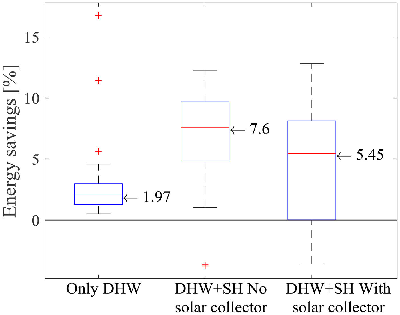
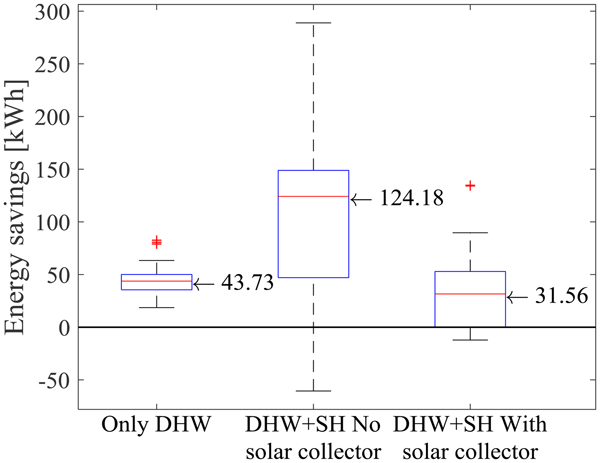
Energy savings made using forecasts are shown in Figures 5–7 using the perfect forecast and the ARIMA forecast obtained with our algorithm, respectively. Perfect forecasts are used here to show the upper limit in terms of energy savings, no matter how precise the forecast is. It is not an absolute upper limit since it does not address the issue of forecast and system control interfacing. For each system configuration, all the 26 profiles have been used to simulate savings. Overall savings are comprised between −3.6% and 17.4% of the total energy consumed. These figures show that the overall saving amount depends on the system but also on the dwelling (and thus the dwellers’ habits) since boxes spread is not negligible.

Fig. 6.

Relative energy savings using ARIMA forecast on the 26 dwellings depending on the considered system.

Fig. 7.

Absolute energy savings using ARIMA forecast on the 26 dwellings depending on the considered system.

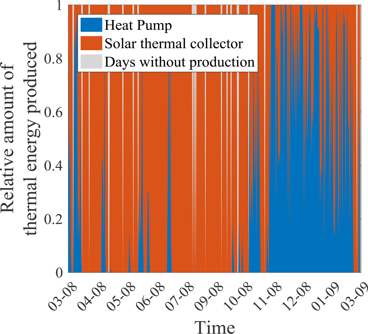
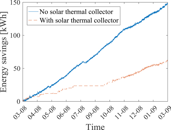
The results also suggest that a solar collector reduces the effectiveness of the technique. Indeed, in summer, a significant part of the energy is provided by the solar collector almost for free (neglecting the energy for a pump). Considering systems without solar collector, heat is provided thanks to HP or resistive devices that are less efficient. Figures 8 and 9 illustrate that point on a particular dwelling. Figure 8 shows that in summer, almost no energy comes from HP when STC is in operation. The consequence on energy saving is shown in Figure 9. No extra savings are achieved during the summer if STC is working while savings steadily increase in the other case.

Fig. 8.

Relative contribution of each source to the thermal energy.

Fig. 9.

Cumulated savings using the HP system with and without STC (configurations 2 and 3).

Even though the efficiency of the resistive system is lower than the others, the energy gains observed using forecast are less important than the case of HP systems. We could expect the gain to be greater (at least) since the production system consumes more energy. Figures 5–7 show that this intuition is neither verified in relative scale nor in absolute. The explanation is that, since the production behavior is very different, the thermal inertia is different; thus, the way the system accounts for forecasts might be less appropriate and yields less savings.

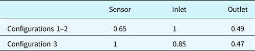
More precisely, in this case, the pipes inlet and outlet positions of the heat production loop and the temperature sensor position are responsible for the thermal inertia discrepancy between systems. These positions are summarized in Table 2 and can be observed in Figures 1 and 2.

Table 2.

Relative position of sensor and pipe/tank connections (1 and 0 are the top and the bottom of the tank, respectively)

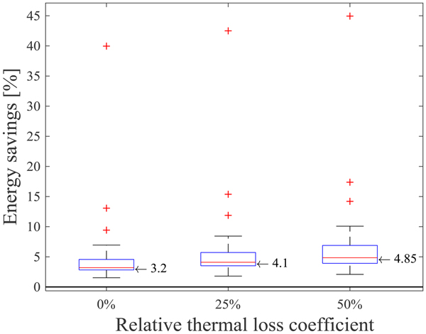
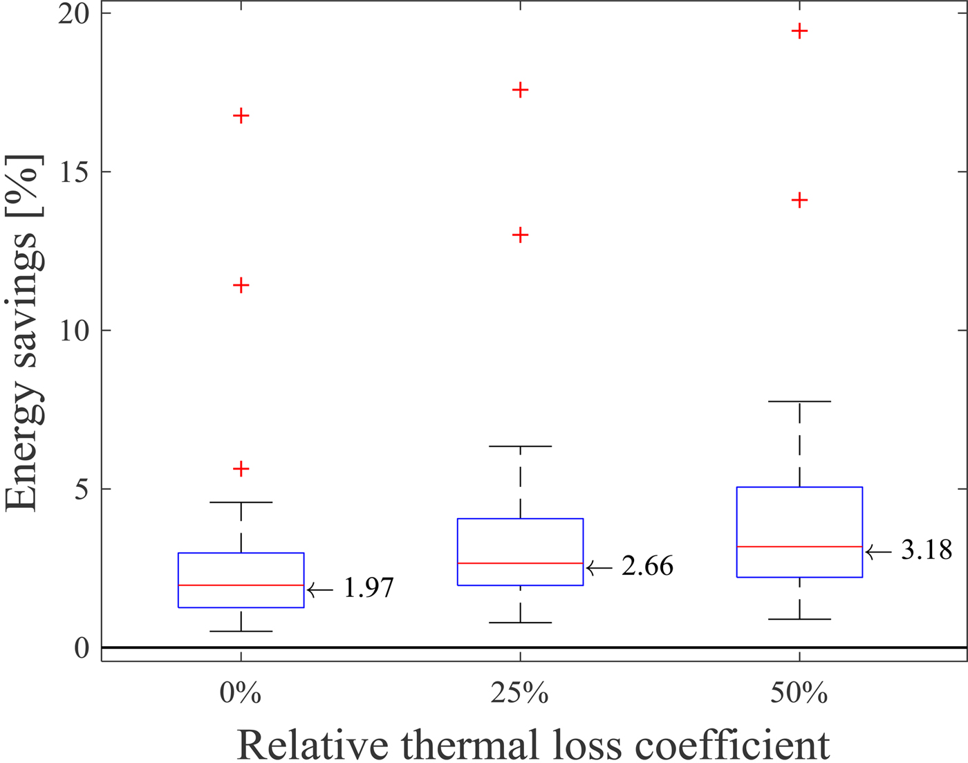
The consequence is that the configuration 1 has short operating cycles that heat a smaller volume of water than configurations 2–3 (the sensor being placed higher). Thus, if DHW is regularly tapped, the average energy of the tank is lower and so is the thermal dissipation compared with configurations 2–3. This is why energy savings are lower in configuration 1. However, this does not hold anymore if there are long periods of absence (>10 days). In this case, which occurs sparsely in our data, without forecast, configuration 1 ends up by heating the whole tank (since DHW is not tapped) and energy losses become as high as in configuration 2. The energy yield is lower in configuration 1, where the anticipative system allows larger savings since it enables shutting down the boiler when no DHW is tapped during the day. The main result to point out is that the characteristics of the boiler can have an impact on how much savings the anticipative system can yield. The algorithm can be tuned to be more efficiently adapted to the boiler. For example, the forecast horizon can be extended or shrunk to adapt to the effective inertia of the boiler and the amplitude of consumption peaks. The effect of thermal insulation of the tank has been studied as well. The reference system has a thermal loss coefficient of 1.08, 10.12, and 2.41 kJ/(h.K) at the top, side, and bottom of the tank, respectively. More information can be found in Bales et al. (Reference Bales, Betak, Broum, Chèze, Cuvillier, Haberl, Hafner, Haller, Hamp, Heinz, Hengel, Kruck, Matuska, Mojic, Petrak, Poppi, Sedlar, Sourek, Thissen and Weidingern.d.). Figures 10 and 11 show the results obtained with the 26 dwellings simulated with different thermal insulations. As a result, poorer insulation allows more savings using the forecast. Indeed, if the tank is well insulated, hot water can be stored longer without suffering from extra dissipation. Thus forecasting the consumption becomes less relevant in terms of energy gain.

Fig. 10.

Relative energy savings using perfect forecast depending on insulation, considering system with resistive heating device. Insulation varies from nominal value (0%) down to 50% less efficiency.

Fig. 11.

Relative energy savings using ARIMA forecast depending on insulation, considering system with resistive heating device. Insulation varies from nominal value (0%) down to 50% less efficiency.

Figures 10 and 11 show that relative savings using consumption forecast are increased by 52% of the baseline value when the insulation is halved. In other words, the relative energy savings increase by 1.65. The effects of the insulation coefficient are slightly exacerbated using ARIMA (up to 61% increase of the baseline value of relative energy saving when the insulation is halved) but the difference might not be significant (relative energy savings increases up to 1.21). So an anticipative strategy is much more adapted with higher energy loss.

Performance of the algorithm and energetic efficiency

Relation between model accuracy and energy savings

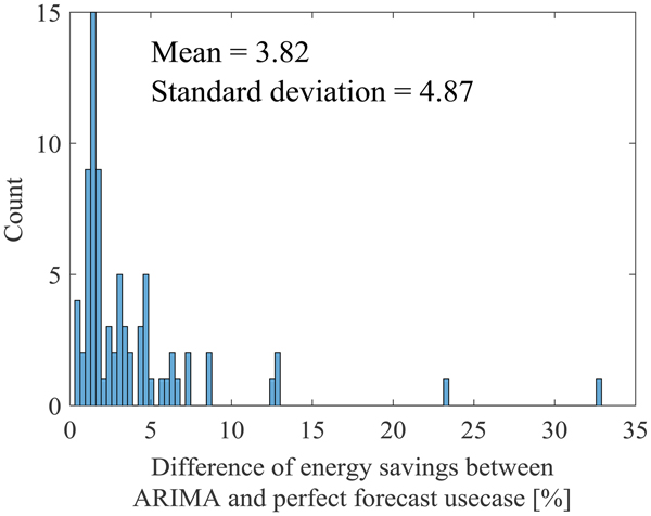
All previous results showed that energy savings depend strongly on the system. It does also depend on the prediction accuracy since using exact forecast yields better results than using ARIMA in Figures 10 and 11. To gain a better insight into the relations between forecast error and energy savings, the energy saving discrepancies observed using ARIMA and perfect forecast are plotted in Figure 12. Energy gain using a perfect forecast is significantly better than using ARIMA forecast. Thus a better accuracy of the model can still improve the energy savings up to 3.8% on average.

Fig. 12.

Distribution of energy savings discrepancies observed using perfect forecast and ARIMA, calculated over the 26 dwellings with the different configurations.

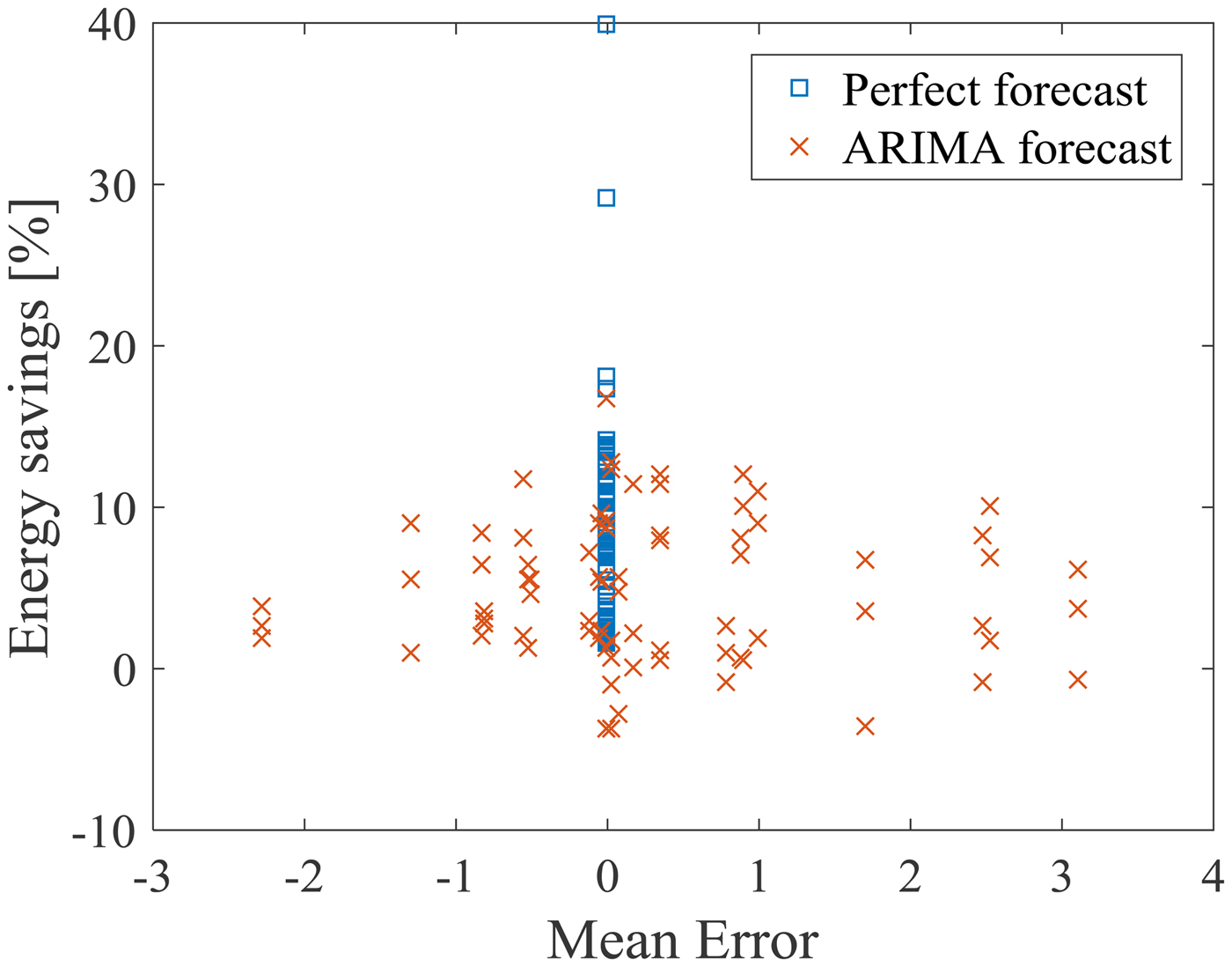
The model mean error (ME) is computed over each simulated year and plotted against energy savings in Figure 13, for each simulated configuration of system and dwelling, using ARIMA and perfect forecast. Errors are computed on the cumulative consumption forecast for the next hour using formula 5,

(5)$${\rm ME} = \displaystyle{1 \over N}\mathop \sum \limits_{t = 1}^N F_t-Y_t$$

where Y _t and F _t denote the observations and forecasts, respectively, with t covering the simulated year. Figure 13 shows that the ME is homogeneously spread around 0 and that a high ME value does not imply lower savings. However, we have seen that the difference between savings using perfect forecast and ARIMA is significantly positive. The conclusion is thus threefold:

• Lower forecast accuracy reduces energy savings

  Fig. 13.

  Energy savings against model mean error.

  

• The system type affects the yield as much as the forecast accuracy

• ME indicator cannot be used as a quantitative estimator of the energy savings.

Considering the interface between forecasts and the control system, the implemented strategy consists in evaluating at each time step the available energy stored in the tank and comparing it with the cumulative consumption forecast over an H hour horizon. The stored energy is adjusted whenever some is missing by turning the production system on. Available energy is computed using four sensors spread along the top half section of the tank. If the stored water is below T _min, then its energy is not taken into account, since this water would not be hot enough if drawn. In our case, H = 1 h and T _min = 48°C. However, depending on the thermal inertia of the system, these parameters could be modified consequently improving or degrading the energy gain obtained using forecast.

Effect of model drift on model accuracy and energy savings

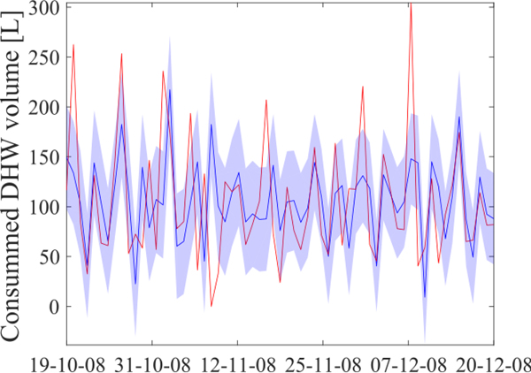
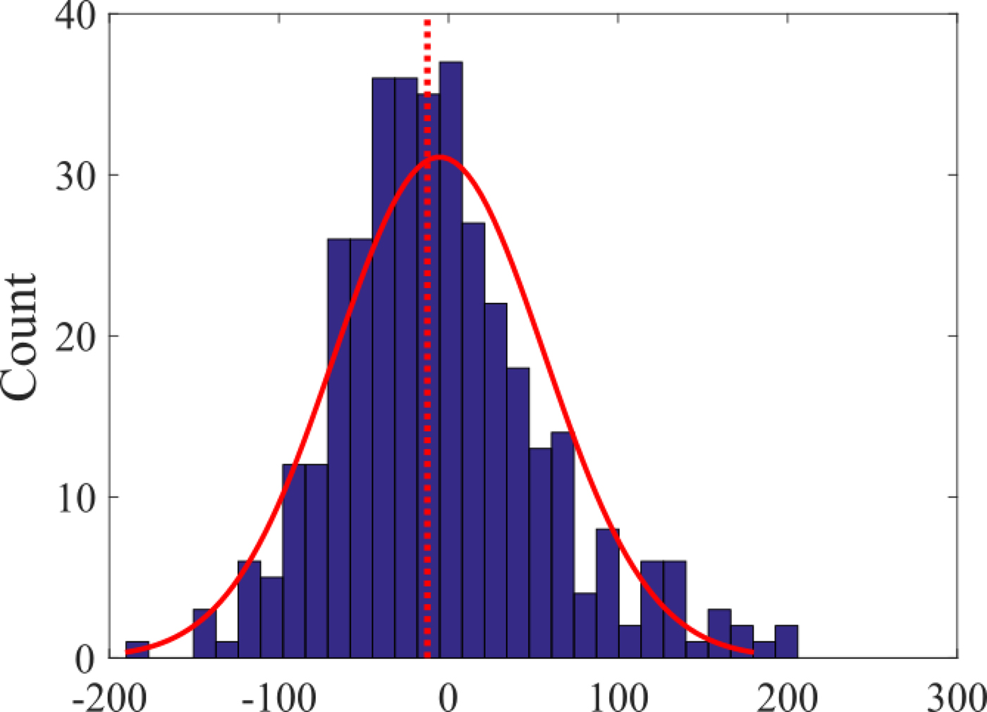
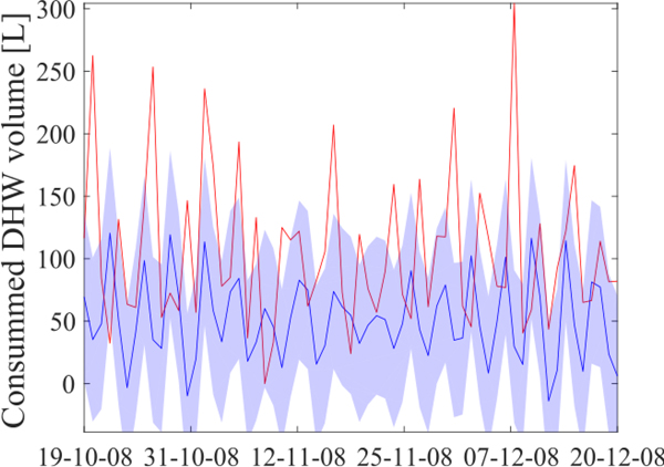
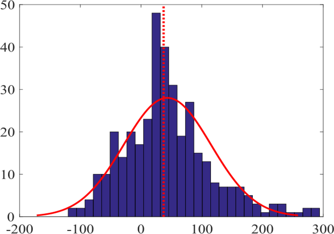
A statistical model trained on a particular data set is suited to forecast consumption of the dwelling from which the training set has been measured. However, nothing ensures that this model would be fitted for another dwelling since it is occupied by other inhabitants with different habits. Moreover within the same dwelling, dwellers can change with time, compromising the fitness of the model. This problem is referred as concept drift. To investigate the amplitude of the error caused by concept drift, models trained on specific dwellings have been used to forecast other dwelling consumptions. Figures 14–17 show the forecasts obtained for dwelling D6 using the models calibrated using DHW consumption of dwelling D6 and D9. The model trained with dwelling D6 is representative of the different models trained with the 26 dwellings (ARIMA coefficients are the closest to coefficient means). The error observed using the model calibrated on D6 to forecast the dwelling D9 consumptions is representative of the errors observed using the same model to forecast all the other dwellings. The figure shows that the concept drift can add a serious bias in the forecast. In this case, the forecast is systematically underestimated. Even though we have seen that large ME is not the most affecting factor on energy gain, the problem of concept drift should be kept in mind and dealt with.

Fig. 14.

Dwelling D6 DHW consumption measured (red lines) and forecast (blue lines) using model calibrated on D6.

Fig. 15.

Histogram of model error Y(d)-F(d) with model calibrated on D6.

Fig. 16.

Dwelling D6 DHW consumption measured (red lines) and forecast (blue lines) using model calibrated on D9.

Fig. 17.

Histogram of model error Y(d)-F(d) with model calibrated on F(d) with model calibrated on D9.

Discussions and guidelines

Improving the energy efficiency of an individual DHW production system using forecast is a challenging task for many reasons. The first challenge not in the scope of this study is to use efficiently a statistical model for DHW forecast through the control. For example, we consider a single dwelling rather than a full district or a town (i.e. for the case of urban heating network) which is easier to forecast thanks to the aggregation of consumptions. Moreover DHW consumption fluctuates over time and is hard to predict since it does not necessarily depend on external factors such as external temperature (Lomet et al., Reference Lomet, Suard and Chèze2015) compared with SH production. This has been studied and published in previous papers (Lomet et al., Reference Lomet, Suard and Chèze2015; Lomet et al., Reference Lomet, Denis, Suard and Chèzen.d.).

However, we focus here on considerations about model embedding into production systems. The study sheds some light about the difficulties of saving energy within anticipative systems (i.e. that uses forecast). First of all, anticipative systems yield greater savings using the tank with poorer insulation than our study case. Second, there is no direct relationship between the initial efficiency of the system and the energy gain that one can expect using forecast. In particular, using STC brings energy to the tank during summer almost for free, thus restricting the gain made using forecast compared with systems without STC. However, the energy gains are even more restricted considering a simple resistive system to produce DHW, whose efficiency is lower than HP systems with and without STC. This has been attributed to the compatibility between forecasts and the system, through the control strategy and the system's characteristics itself. For example, the position of the pipes inlet and outlet and the thermal sensor has been pointed out as being responsible for shorter heating cycles in the system configuration 1 leading to lower energy stored and thus less dissipation for most of the dwellings. Thus the production system characteristics have a large impact on energy savings. Finally the energy gain also strongly depends on the dwelling considered and dwellers habits. Thus no pledge about the saving amount can be held without knowing the DHW production system and the dwellers habits, with the strategy we used to interface forecasts and the control system.

The strength of this forecast model, compared with the state of the art presented earlier, is that it is lightweight and thus embeddable in the production system. Moreover, it does not depend on external parameters and only needs the history of DHW consumption to be able to run, making it flexible and easily embeddable. Another model, more sophisticated, provides greater accuracy but in this work we have shown that the accuracy of our model is not the main lever to save more energy with anticipative systems. However, attention must be paid to production system characteristics and how the forecast is integrated within the DHW production management system. Moreover the period of learning data set should be representative of global usage.