Implications
The availability of genomic information demands proper assessment of its impact on practical horse breeding programs. Accuracies of conventional breeding values do not increase significantly until a stallion is aged 8 to 12 years and his progeny enters competition. We showed that additional genomic information considerably increases the accuracy of breeding values estimated for foals, young horses without own performance, and horses without progeny performance. Therefore, genomic selection (GS) enables selection at an earlier stage, shortening generation intervals and opening room for increased genetic progress. Our results indicate that horse breeding organizations could likely benefit from the application of GS.
Introduction
Sport horse breeding programs are characterized by long generation intervals and suboptimal selection intensities (Philipsson et al., Reference Philipsson, Árnason and Bergsten1990; Niemann, Reference Niemann2009) because of the lack of efficient selection criteria early in life. Estimated breeding values (EBVs) including information on own performance and on progeny performance are generally not available until a horse is 8 to 12 years old (German Equestrian Federation, 2008).
Genomic selection (GS) has the potential to substantially improve existing breeding strategies. The notion of GS was formulated by Meuwissen et al. (Reference Meuwissen, Hayes and Goddard2001) and is being implemented in dairy cattle breeding programs (Hayes et al., Reference Hayes, Bowman, Chamberlain and Goddard2009). The benefit of GS to conventional breeding programs has been demonstrated for dairy cattle (Schaeffer, Reference Schaeffer2006; König et al., Reference König, Simianer and Willam2009) and for pigs (Simianer, Reference Simianer2009). A substantial increase in genetic gain was found for breeding programs characterized by long generation intervals, and those focusing on lowly heritable, functional traits (König et al., Reference König, Simianer and Willam2009). Both findings support the demand to evaluate the potential of GS for horse breeding programs.
The aims of our study were to: (i) evaluate the impact of genomic breeding values (GEBVs) on the accuracy of EBVs and on the relative selection response by applying selection index theory; (ii) develop a strategy to address the practical problem of how to combine different types of EBVs (e.g. GEBV and EBVs available from different countries) in an overall breeding goal.
Material and methods
The methodology of combining phenotypic observations (y) and the single nucleotide polymorphism (SNP) genotype as a marker trait (m) via selection index theory was developed by Dekkers (Reference Dekkers2007). Application of this methodology was put into practice by König and Swalve (Reference König and Swalve2009) to evaluate genomic breeding strategies in dairy cattle breeding programs. The present study, this method was extended to specific scenarios relevant for selection decisions in horse breeding programs. Evaluation criteria were the correlation between aggregate genotype and selection index, referred to as accuracy of the EBV (rTI ), as well as the relative selection response (RSR), which was calculated applying the formula

with ΔG being the selection response per generation. In order to assess the impact of GS on practical situations, all scenarios were investigated for a lowly heritable, functional trait and a trait of high heritability. As an example for a lowly heritable trait, susceptibility to osteochondrosis (OC), with a heritability of 0.15 (Pieramati et al., Reference Pieramati, Pepe, Silvestrelli and Bolla2003; Schober, Reference Schober2003), was chosen. OC can cause disorders of chondral growth. When diagnosed, it reduces the horse's sales value considerably (Van Hoogmoed et al., Reference Van Hoogmoed, Snyder, Thomas and Harmon2003; Stock and Distl, Reference Stock and Distl2007). The quality of trot (h 2 = 0.52; Jaitner and Reinhardt, Reference Jaitner and Reinhardt2008) is highly correlated to the other gaits and to the rideability (Schade, Reference Schade1996; Thorén Hellsten et al., Reference Thorén Hellsten, Viklund, Koenen, Ricard, Bruns and Philipsson2006), and therefore represents an important high heritability trait not only for dressage horses.
Scenario I: Genotyped young horse without own performance
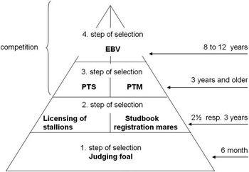
Scenario I was designed considering animals without own performance according to the first step of selection in the breeding scheme of the German Riding Horse (Figure 1). At the age of 6 months, foals are inspected by the breeding associations. Many breeders decide whether or not to castrate the young stallion based on these first results, even though the correlations between results of foal inspection and subsequent studbook inspections are low (Schorm, Reference Schorm1983). A high proportion of male foals is castrated at a very young age, resulting in low selection intensities in subsequent steps of selection (Philipsson et al., Reference Philipsson, Árnason and Bergsten1990; von Lengerken and Schwark, Reference von Lengerken and Schwark2002). Scenario I is also valid to achieve improvements in selection of young mares without own performance, for example, to select mares as potential donors for embryo transfer (ET). Hence, we constructed a scenario for the genomic era where the SNP genotype of the foal, as well as the performances of the dam and of the sire, was used as information sources in the index.
Pyramid structure of the breeding program of the German Riding Horse. EBV = estimated breeding value; PTS = performance test stallions; PTM = performance test mares.

The (co)variance matrix P of index sources was

The first line of P refers to the marker genotype of the foal, the second line refers to the phenotypic performance of the sire and the third line corresponds to the phenotypic performance of the dam. According to Lynch and Walsh (Reference Lynch and Walsh1998), the heritability of the SNP genotype was fixed to a value of 1, which entails identical values for both phenotypic and genetic variance of the marker trait ( ). Variances for m were calculated using equation (1):

where rmg
denotes the correlation between the breeding value estimated from the SNP genotype and the true breeding value (= accuracy of GEBV), and  is the additive-genetic variance of the trait.
 is the phenotypic variance of the trait. The covariance σam
between marker genotype m and phenotype y is described by the general equation (2):

with aij being the coefficient of relationship between animal i used in the index and animal j in the aggregate genotype. For this scenario, the coefficient of relationship between foal i and its dam and sire j was 0.5.
Covariances between traits in the index and traits in the breeding goals were included in matrix G, which was defined as

The first line of G refers to the marker genotype of the foal, the second line refers to phenotypic performance of the sire and the third line represents the phenotypic performance of the dam. The columns correspond to the GEBV estimated from the marker genotype m and to the conventional breeding value of the phenotypic trait y. Matrix C was the matrix for variances and covariances of breeding values, that is,

As the SNP genotype was considered as an auxiliary trait, the economic weight was put on the phenotypic performance, which resulted in vector w being

The variance of the aggregate genotype (T) was  , and the variance of the index (I) was
 . These variances are essential to calculate
 .
Scenario II: Genotyped horse with own performance
In scenario II, the selection index was extended for a genotyped horse with own performance, but without progeny information. Such a scenario corresponds to step 3 of selection (Figure 1), that is, to young stallions or mares at the age of 4 to 7 years, which have accomplished performance testing. Information for the dam and for the sire was considered as done in scenario I. Matrix P of phenotypic (co)variances was

and matrix G was written as

Equations (1) and (2) were applied to calculate variance and covariance components for matrices P and G. The vector w of economic weights and the (co)variance matrix C for breeding values were identical to w and C in scenario I.
Scenario III: Genotyped horse with own performance and performance of progeny
The fourth step of selection in a conventional breeding program is the estimation of breeding values (Figure 1). In order to estimate highly reliable EBVs, progeny records are needed. Therefore, this scenario corresponds to stallions at the age of 8 to 12 years. As a consequence, five index sources were considered in this scenario: records of a varying number of progeny (5, 50 or 100, respectively), the SNP genotype of the stallion, the own performance of the stallion and again the performance of the dam and the sire. Hence, matrix P was

and matrix G was

Again, the vector w of economic weights and the (co)variance matrix C for breeding values were identical to w and C in scenario I.
Scenario IV: Combination of breeding values into a combined index
Scenarios I to III were constructed to evaluate the potential of additional SNP information in terms of rTI or relative selection response. The following approach addresses the question how to combine different EBVs with different accuracies and different correlations among each other into a combined index, which is constructed to match an overall breeding goal. This would be of use, for example, in case EBVs from different countries were available for a stallion. Another application would include the merging of conventional EBVs with GEBVs or joining EBVs measured at different stages of the horse's life, as was assumed in this scenario. Methodology is also based on selection index calculations, but using EBVs rather than phenotypic observations.
In this scenario, a combined index (T), illustrating an overall breeding goal, is composed of three different EBVs (TBVs), which are considered as traits of T. Hence, the overall index of an animal k was

According to selection index theory, b-values were calculated as

with matrices P and G as explained below.
For each TBV, a separate type of EBV is available as information source: (1) an integrated breeding value (IEBV) incorporating all available information on relatives of a stallion, as well as progeny information, which commonly has a high accuracy (rTI ) and in this example is arbitrarily set to 0.85 for all runs. Because progeny information is considered, IEBVs are only available later in life; (2) an EBV including the result of the stallion's performance test as well as the results of its performance tested male relatives (stallion estimated breeding value, SEBV). Due to less information and estimation earlier in life, the accuracy of SEBVs is generally lower than for IEBVs, and therefore we have chosen the values of 0.5 and 0.8, respectively; and (3) a GEBV with accuracy varying from 0.1 to 0.9. The correlation between IEBV and SEBV was set to 0.95, and for all TBVs equal economic weights per genetic standard deviation were assumed. In a second run, the correlation between IEBV and SEBV was reduced to 0.5. Notations for matrices were chosen in analogy to index calculations used above. The standard deviation of the EBV for a trait i was

where  denotes the standard deviation of the breeding value TBVi
, which was used in the overall index and
 is the correlation between EBVi
and TBVi
, or in other words the accuracy of the
 . The correlation between an EBVi
and an EBVj
is

This information is needed to compute matrix P, the variance–covariance matrix for n EBVs:

Covariances between an EBVi and an EBVj were calculated using the following formula:

Matrix C, the quadratic variance–covariance matrix for m TBVs in the overall index, was

Covariances between TBVi and TBVj were calculated by using the following formula:

Matrix G of dimension n × m is the covariance matrix between the n EBVs used in the index and the m TBVs used in the aggregate genotype (= breeding goal):

Those covariances in G were calculated by using the formula:

Hence, the individual weighting factor b of an EBVi for an animal in the overall breeding goal depends on the accuracy of this EBV. Correlations among TBVs in the breeding goal, as well as economic weights w, are equal for all groups of animals.
The accuracy of Tk was

Results and discussion
Estimation of SNP effects within a calibration group, and transferring those estimates to animals in the whole population, is the key feature of GS methodology. The availability of 50-K SNP chip technology, as well as the recent release of the horse genome sequence (Wade et al., Reference Wade, Giulotto, Sigurdsson, Zoli, Gnerre, Imsland, Lear, Adelson, Bailey, Bellone, Blöcker, Distl, Edgar, Garber, Leeb, Mauceli, MacLeod, Penedo, Raison, Sharpe, Vogel, Andersson, Antczak, Biagi, Binns, Chowdhary, Coleman, Della Valle, Fryc, Guérin, Hasegawa, Hill, Jurka, Kiialainen, Lindgren, Liu, Magnani, Mickelson, Murray, Nergadze, Onofrio, Pedroni, Piras, Raudsepp, Rocchi, Røed, Ryder, Searle, Skow, Swinburne, Syvänen, Tozaki, Valberg, Vaudin, White and Zody2009), provides the framework to estimate highly reliable GEBVs analogous to dairy cattle (e.g. VanRaden et al., Reference VanRaden, Van Tassel, Wiggans, Sonstegard, Schnabel, Taylor and Schenkel2009). The extent of linkage disequilibrium (LD) was analyzed by Corbin et al. (Reference Corbin, Blott, Swinburne, Vaudin, Bishop and Woolliams2010) for the Thoroughbred horse. Owing to the high LD, the authors concluded that GS could be applied in the observed population. However, strength of LD as a function of the effective population size (N e) may be lower in European sport horse breeds compared with the Thoroughbreds (N e = 100). For example, in the Hanoverian Warmblood, N e was estimated to be 372 (Hamann and Distl, Reference Hamann and Distl2008). Wade et al. (Reference Wade, Giulotto, Sigurdsson, Zoli, Gnerre, Imsland, Lear, Adelson, Bailey, Bellone, Blöcker, Distl, Edgar, Garber, Leeb, Mauceli, MacLeod, Penedo, Raison, Sharpe, Vogel, Andersson, Antczak, Biagi, Binns, Chowdhary, Coleman, Della Valle, Fryc, Guérin, Hasegawa, Hill, Jurka, Kiialainen, Lindgren, Liu, Magnani, Mickelson, Murray, Nergadze, Onofrio, Pedroni, Piras, Raudsepp, Rocchi, Røed, Ryder, Searle, Skow, Swinburne, Syvänen, Tozaki, Valberg, Vaudin, White and Zody2009) found unusually high LD in Thoroughbreds compared with other horse breeds. Nevertheless, GS should be feasible, because strength of LD across several horse breeds (Wade et al., Reference Wade, Giulotto, Sigurdsson, Zoli, Gnerre, Imsland, Lear, Adelson, Bailey, Bellone, Blöcker, Distl, Edgar, Garber, Leeb, Mauceli, MacLeod, Penedo, Raison, Sharpe, Vogel, Andersson, Antczak, Biagi, Binns, Chowdhary, Coleman, Della Valle, Fryc, Guérin, Hasegawa, Hill, Jurka, Kiialainen, Lindgren, Liu, Magnani, Mickelson, Murray, Nergadze, Onofrio, Pedroni, Piras, Raudsepp, Rocchi, Røed, Ryder, Searle, Skow, Swinburne, Syvänen, Tozaki, Valberg, Vaudin, White and Zody2009) is comparable to LD in Holstein cattle (Qanbari et al., Reference Qanbari, Pimentel, Tetens, Thaller, Lichtner, Sharifi and Simianer2010), where GS was implemented successfully. First practical investigations in terms of estimation of GEBVs in horses are carried out for Franches-Montagnes horses in Switzerland (Hasler et al., Reference Hasler, Flury, Menet, Haase, Leeb, Simianer, Poncet and Rieder2011).
Scenario I: Genotyped young horse without own performance
Owing to insufficient sources of information at this stage of selection, accuracies of breeding values estimated for young horses are particularly low, especially for low heritability traits. Selection of foals at this early point in time reduces generation intervals, but is associated with a higher risk for practical breeders. Model calculations by Schade (Reference Schade1996) showed that genetic gain is reduced by 70% if stallions are used for matings before being performance tested. This is probably due to the fact that the phenotype itself, that is, riding quality, cannot be tested at this early point in time. Particularly with regard to castrating, there is a high risk of unfortunate selection decisions as long as there is no information on own performance available.
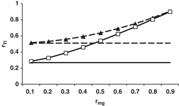
Only including phenotypic records from the sire and the dam of the foal in the index results in rTI
= 0.27 for OC (Figure 2). As known from selection index theory, additional information from further close relatives of the foal would increases rTI
only marginally. In contrast, a distinct gain of accuracies can be achieved when including the SNP genotype in addition to the sire's and dam's performance, even for low accuracies of GEBVs (rmg
) in combination with a low heritability (Figure 2). For rmg
= 0.3, the additional information of the SNP genotype increases rTI
to 0.39. Extremely high rmg
of 0.8, or even higher, enable similar rTI
for the low and the high heritability trait (rTI
= 0.81 to 0.91). However, when referring to other species, for example, dairy cattle, accuracies of GEBVs are substantially higher for production traits compared with fertility, somatic cell score or longevity (VanRaden et al., Reference VanRaden, Van Tassel, Wiggans, Sonstegard, Schnabel, Taylor and Schenkel2009). Nevertheless, on the basis of results from simulation studies or deterministic predictions (Calus et al., Reference Calus, Meuwissen, de Roos and Veerkamp2008; Daetwyler et al., Reference Daetwyler, Pong-Wong, Villanueva and Woolliams2010), a correlation of rmg
= 0.5 should be feasible also for GS for functional traits in horses. Such a crucial value doubles rTI
at this very early point of selection (Figure 2) compared with the accuracy of the conventional index. When additionally considering economical aspects, even rmg
lower than 0.5 enable additional gain in terms of return of investment for pig breeding programs (Simianer, Reference Simianer2009), or in terms of breeding profit for dairy cattle breeding programs (König et al., Reference König, Simianer and Willam2009). Thus, pre-selection of genotyped foals can be used for the identification of promising selection candidates very early and therefore helps to avoid improper castrating decisions. Until further testing, the issue of temporary breeding permissions may contribute to shorten generation intervals and is already practised by several organizations. Those breeding permissions are valid from the stallion's licensing carried out at the age of  years and allow a limited number of matings until the stallion is performance tested at the age of 3 or 4 years. However, the accuracy and effectiveness of this practice could be improved by considering GEBVs as additional information source.
Correlation between index and aggregate genotype (rTI ) in dependency of accuracy of GEBV (rmg ) for a genotyped horse without own performance (Scenario I). Dashed line with black triangles: trot (h 2 = 0.52); solid line with white squares: OC (h 2 = 0.15). Parallel lines to x-axis: conventional accuracies not including GEBVs in the index, that is, dashed line for trot and solid line for OC. GEBV = genomic estimated breeding value; OC = osteochondrosis.

According to Schaeffer (Reference Schaeffer2006), more accurate breeding values on the dam side of selection can be achieved when genotyping females. This can be of economic importance when choosing young females without own performance as donors for ET, which still is an expensive biotechnology. New commercial reproductive technologies such as ET have been adopted by some horse breeding associations. Long et al. (Reference Long, Walker, Wang and Westhusin2003) focused on two examples, the American Quarter Horse Association and the United States Polo Association. Advantages of ET will increase with decreasing generation intervals, provided that sufficiently reliable EBVs of young mares are available. For this specific case in horse breeding, the combination of both reproduction technologies and molecular genetic tools is a powerful approach to further increase selection response (e.g. Spelman and Garrick, Reference Spelman and Garrick1998).
Scenario II: Genotyped horse with own performance
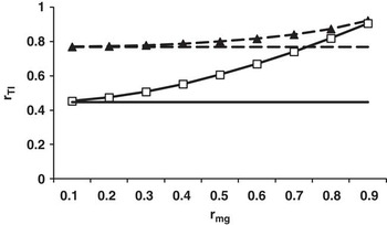
The higher the basic result for rTI without considering genomic information, the lower the gain in rTI when including additional SNP information in the index (comparison of Figures 2 and 3).
Correlation between index and aggregate genotype (rTI ) in dependency of accuracy of GEBV (rmg ) for a genotyped horse with own performance and performance of parents (Scenario II). Dashed line with black triangles: trot (h 2 = 0.52); solid line with white squares: OC (h 2 = 0.15). Parallel lines to x-axis: conventional accuracies not including GEBVs in the index, that is, dashed line for trot and solid line for OC. GEBV = genomic estimated breeding value; OC = osteochondrosis.

The conventional index sources own performance, performance of sire and performance of dam result in rTI = 0.45 for h 2 = 0.15 (Figure 3). Including additionally a GEBV with rmg = 0.5 in the index, rTI increased by 40%. For rmg = 0.9, relative selection response (not shown) is doubled to a value of 2.03. Hence, in scenario II, the benefit of GS in terms of gains in rTI is substantial, in particular for the lowly heritable, functional trait.
Generally, rTI cannot drop below rmg (König and Swalve, Reference König and Swalve2009). As a practical consequence, provided that rmg is 0.7 or higher, rTI reaches at least the same level as can be obtained by running performance testing. For example, for rmg = 0.8 and h 2 = 0.15, rTI for the combination of the SNP genotype and own performance is 0.82. Formulas developed by Stricker and Fernando (Reference Stricker and Fernando2008) or by Daetwyler et al. (Reference Daetwyler, Villanueva and Woolliams2008 and Reference Daetwyler, Pong-Wong, Villanueva and Woolliams2010) can be used to derive rmg dependent on the number of genotyped animals.
However, reliable phenotypes are an essential pre-requisite to derive reliable SNP effects. The most effective source of data for genetic evaluation of young stallions and their parents is phenotyping carried out in the form of performance tests on station (Gerber Olsson et al., Reference Gerber Olsson, Árnason, Näsholm and Philipsson2000; Thorén Hellsten et al., Reference Thorén Hellsten, Viklund, Koenen, Ricard, Bruns and Philipsson2006). Continuous phenotyping in this format and frequent re-estimation of SNP effects within a calibration group are required because the accuracy of GEBVs is declining over generations as shown in simulation studies by Habier et al. (Reference Habier, Fernando and Dekkers2007). This is due to a decreasing relationship between calibration group and selection candidates, as well as due to decay in LD between SNP-markers and surrounding quantitative trait loci caused by recombination events (Sonesson and Meuwissen, Reference Sonesson and Meuwissen2009). In addition, as priorities in breeding goals change or new assessment techniques become available, from time to time new phenotypes (e.g. König von Borstel et al., Reference König von Borstel, Euent, Graf, König and Gauly2011) may be introduced into the breeding program, requiring estimation and calibration of SNP effects for these new traits.
In order to keep generation intervals as short as possible, breeding organizations should encourage the use of young stallions. The accuracy of EBVs of performance tested stallions can still be enhanced by including genomic information.
Scenario III: Genotyped horse with own performance and performance of progeny
Generally, for the estimation of highly reliable EBVs, the availability of progeny records is of major importance. This implies that stallions are at the age of 8 years or even older once their EBVs reach high accuracies of 0.92 to 0.99 (German Equestrian Federation, 2008). Dubois and Ricard (Reference Dubois and Ricard2007) focused on the problems of long generation intervals due to extended progeny testing systems, and they encouraged breeders to use younger stallions with a reduced number of progeny as a compromise.
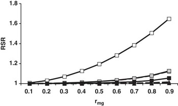
Additional gain in rTI from GEBV is relatively low when performance of parents, own performance and progeny records are available as index sources. This finding is illustrated by the relative selection response (Figure 4). For the highly heritable trait and 50 or 100 progeny records, the value of RSR is, independent from rmg , close to 1. This implies negligible gain when considering the GEBV as additional index information. For the lowly heritable trait and 50 or 100 progeny records, and for the highly heritable trait and five progeny records, RSR ranged from 1.06 to 1.13 for rmg = 0.9. Substantial gain in rTI in scenario III was found only for the lowly heritable trait and five offspring, leading to an RSR of 1.65.
Relative selection response for a genotyped horse with own performance, performance of parents, and a different number of progeny in dependency of accuracy of GEBV (rmg ). Dashed lines with triangles: trot (h 2 = 0.52); solid lines with squares: OC (h 2 = 0.15). White triangles or squares: five progeny; gray triangles or squares: 50 progeny; black triangles or squares: 100 progeny. GEBV = genomic estimated breeding value; OC = osteochondrosis.

Methodology developed for scenario III can additionally be used to derive the optimal number of progeny records to achieve a pre-defined rTI . Additional progeny records contribute to realize a high rTI for an index considering lowly heritable traits and genomic information with moderate rmg in the range from 0.4 to 0.7.
A crucial point for the practical implementation and ultimate success of GS will be the acceptance of GEBV by practical breeders, as well as the additional cost component for genotyping sport horses. Applied selection strategies in horse breeding programs traditionally have a strong focus on phenotypic performances rather than EBVs (Koenen et al., Reference Koenen, Aldridge and Philipsson2004). Beyond dressage and show jumping, breeders have the opportunity to use GEBVs of health traits, for example, OC, for selection decisions. Van Hoogmoed et al. (Reference Van Hoogmoed, Snyder, Thomas and Harmon2003) showed that radiographic findings of OC severely reduce the sales value of a horse. Some further studies, for example, Stock and Distl (Reference Stock and Distl2007) investigated the correlations between radiographic findings and performance traits in warmblood riding horses. They concluded that riding horse performance will likely benefit from the reduction of prevalence of radiographic findings. Hence, all available tools should be applied to reduce incidence of disorders.
Scenario IV: Combination of breeding values into a combined index
Application of scenarios I to III is appropriate for such situations where detailed information for selection index calculations are available, for example number of animals within selection groups, phenotypic parameters and genetic parameters. In general, availability of those parameters is guaranteed within an own breeding program or on the national scale. A major requirement for the practical implementation of GS in sport horse breeding programs is the setup of a calibration group for the estimation of SNP effects. For achieving adequate accuracies of the GEBV, it will be beneficial for breeding organizations to cooperate in this matter, like exemplified by the European breeding organizations of Holstein–Friesian cattle (Lund et al., Reference Lund, de Roos, de Vries, Druet, Ducrocq, Fritz, Guillaume, Guldbrandtsen, Liu, Reents, Schrooten, Seefried and Su2010). A calibration group composed of animals being registered in different breeding organization would be justified by the extensive genetic exchange between breeding populations within Germany, as well as between European countries (Koenen et al., Reference Koenen, Aldridge and Philipsson2004). Scenario IV could be applied for the combination of single breeding values from different countries in an index constructed to match an overall breeding goal. There is also the possibility to use stallions from, for example, Sweden or the Netherlands in German breeding programs, and those stallions have different sources of EBVs. Hence, addressing the question of an optimal combination of EBVs is important.
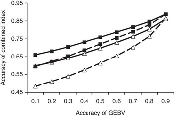
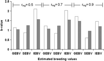
Results in terms of  and weighting factors (b-values) for the combination of GEBV, IEBV and SEBV by altering rmg
are depicted in Figures 5 and 6, respectively. Independently of the accuracy for SEBV, that is, 0.8 v. 0.5, accuracy of the combined index substantially increases with increasing rmg
. For different accuracies of SEBV, the gap in accuracies for the combined index decreases with increasing rmg
(Figure 5). This is due to the impact of highly accurate GEBVs explaining most of the genetic variance of the aggregate genotype. Hence, for high accuracies of GEBVs, further correlated information sources only marginally improve the accuracy of the aggregate breeding value.
Accuracy of the combined index including GEBV, IEBV and SEBV in dependency of accuracies of GEBV (rmg ) for equal economic weights per genetic s.d. (solid lines: correlation between SEBV and IEBV = 0.95; dashed lines: correlation between SEBV and IEBV = 0.50; black squares: accuracy of SEBV = 0.8; white triangles: accuracy of SEBV = 0.5; accuracy of IEBV = 0.85 for all scenarios). GEBV = genomic estimated breeding value; IEBV = integrated estimated breeding value; SEBV = stallion estimated breeding value.

Weighting factors (b-values) for the combination of GEBV, IEBV and SEBV in a combined index in dependency of accuracies of GEBV (rmg ) for equal economic weights per genetic s.d. (white bars: accuracy of SEBV = 0.5; black bars: accuracy of SEBV = 0.8; accuracy of IEBV = 0.85 for all scenarios). The correlation between IEBV and SEBV was 0.95. GEBV = genomic estimated breeding value; IEBV = integrated estimated breeding value; SEBV = stallion estimated breeding value.

However, in reality accuracies of GEBVs will not be high enough to justify the complete abolishment of own-performance testing within horse breeding programs, such as the performance test for stallions. Moreover, performance testing provides phenotypic data that are of major importance for the re-estimation of marker effects in genomic breeding programs. For those reasons, the most likely breeding strategy remains a combination of both GS and performance testing. Considerable, earlier selection of male and female animals for breeding is possible because of the estimation of GEBVs for animals without phenotypic data.
Conclusions
On the basis of our results, application of GS can contribute to well-founded selection decisions within several selection stages of equine breeding programs particularly with regard to lowly heritable (e.g. functional) traits. For animals with a large number of progeny records available, additional gain in accuracy from GEBV is small. Accurate selection of genotyped young horses without own or progeny performance leads to a considerable reduction in generation intervals, and thereby increases the genetic response.
In order to apply GS in practice, breeding organizations will have to convince horse breeders that GS can be a valuable tool to increase selection response.
Acknowledgments
We would like to thank the German Ministry of Education and Research for the financial support of the program FUGATO + brain, which is also supported by the five horse breeding associations for Hanoverian, Trakehner, Oldenburger, Holsteiner and Westfalian horses.