2.1. The point vortex model

The Hamiltonian point vortex model describes the motion in $\mathscr{D}$ of $N$ vortices of infinitesimal size with circulations ${\it\Gamma}_{i}$  ( $i=1,\ldots ,N$ ). Here, we will be mainly concerned with the case of a neutral vortex gas, satisfying

(2.1) $$\begin{eqnarray}\displaystyle \mathop{\sum }_{i=1}^{N}{\it\Gamma}_{i}=0, & & \displaystyle\end{eqnarray}$$

this being the system of most relevance to numerical simulations of 2D turbulence. Many of the results below can be generalised to the non-neutral case, i.e. flows with non-zero circulation, but the results are more complicated and will be reported elsewhere. The vortex locations $\boldsymbol{x}_{i}=(x_{i}\;y_{i})^{\text{T}}\in \mathscr{D}$ evolve according to Hamilton’s equations (e.g. Newton Reference Newton2001)

(2.2a,b ) $$\begin{eqnarray}\displaystyle {\it\Gamma}_{i}\,\frac{\text{d}x_{i}}{\text{d}t}=-\frac{\partial H}{\partial y_{i}},\quad {\it\Gamma}_{i}\,\frac{\text{d}y_{i}}{\text{d}t}=\frac{\partial H}{\partial x_{i}},\quad i=1,\ldots ,N, & & \displaystyle\end{eqnarray}$$

where the Hamiltonian (Lin Reference Lin1941a ) is given by

(2.3) $$\begin{eqnarray}H(\boldsymbol{x}_{1},\ldots ,\boldsymbol{x}_{N})=-\frac{1}{2}\mathop{\sum }_{i=1}^{N}\mathop{\sum }_{j=1,\,j\neq i}^{N}{\it\Gamma}_{i}{\it\Gamma}_{j}G(\boldsymbol{x}_{i},\boldsymbol{x}_{j})-\frac{1}{2}\mathop{\sum }_{i=1}^{N}{\it\Gamma}_{i}^{2}g(\boldsymbol{x}_{i},\boldsymbol{x}_{i}).\end{eqnarray}$$

Here $G(\boldsymbol{x},\boldsymbol{x}^{\prime })$ is the Green’s function of the first kind of the Laplacian operator in $\mathscr{D}$ , satisfying

(2.4a,b ) $$\begin{eqnarray}{\rm\nabla}^{2}G(\boldsymbol{x},\boldsymbol{x}^{\prime })={\it\delta}(\boldsymbol{x}-\boldsymbol{x}^{\prime }),\quad G(\boldsymbol{x},\boldsymbol{x}^{\prime })=0\quad \text{on}~\partial \mathscr{D},\end{eqnarray}$$

where the Laplacian ${\rm\nabla}^{2}$ acts on $\boldsymbol{x}$ only, $\partial \mathscr{D}$ denotes the boundary of $\mathscr{D}$ , and

(2.5) $$\begin{eqnarray}\displaystyle g(\boldsymbol{x},\boldsymbol{x}^{\prime })=G(\boldsymbol{x},\boldsymbol{x}^{\prime })-\frac{1}{2{\rm\pi}}\log |\boldsymbol{x}-\boldsymbol{x}^{\prime }|. & & \displaystyle\end{eqnarray}$$

Note that the terms involving $g$ in (2.3) only require the evaluation of the so-called Robin function $r(\boldsymbol{x})=g(\boldsymbol{x},\boldsymbol{x})$ in which the position arguments of $g$ are set to be equal. The Robin function describes the interaction of each individual vortex with the domain boundary, and in some domains it can be expressed as the streamfunction induced by one or more ‘image’ vortices outside the domain, evaluated at the location of the vortex itself. A solitary vortex in $\mathscr{D}$ will move along a path with $r(\boldsymbol{x})=\text{const}$ .

The statistical mechanics of the system (2.2) will be discussed next.

2.2. Microcanonical statistical mechanics

Provided that $\mathscr{D}$ has no continuous symmetries, for example $\mathscr{D}$ is not a circle, a periodic channel or a doubly periodic domain, the Hamiltonian $H$ is the only known conserved quantity of the motion. Provided ergodicity can be assumed, an aspect that will be discussed briefly in § 4.2 below (see also Weiss & McWilliams Reference Weiss and McWilliams1991), the relevant statistical ensemble for the dynamical system (2.2) is the microcanonical ensemble consisting of all vortex configurations with a fixed energy $H=E$ . Hereafter, angle brackets will be used to denote the microcanonical ensemble average, e.g.  $\langle {\it\omega}(\boldsymbol{x})\rangle$ for the average of the vorticity distribution

(2.6) $$\begin{eqnarray}{\it\omega}(\boldsymbol{x})=\mathop{\sum }_{i=1}^{N}{\it\Gamma}_{i}{\it\delta}(\boldsymbol{x}-\boldsymbol{x}_{i}).\end{eqnarray}$$

Thermodynamic quantities can be obtained using the density-of-states function, i.e. the classical measure of the number of microstates occupying each energy shell, which for given vortex circulations ${\it\bf\Gamma}=({\it\Gamma}_{1},\ldots ,{\it\Gamma}_{N})^{\text{T}}$ is defined as

(2.7) $$\begin{eqnarray}W_{{\it\bf\Gamma}}(E)=\frac{1}{A^{N}}\displaystyle \int _{\mathscr{D}^{N}}{\it\delta}(E-H(\boldsymbol{x}_{1},\ldots ,\boldsymbol{x}_{N}))\,\text{d}\boldsymbol{x}_{1}\cdots \text{d}\boldsymbol{x}_{N},\end{eqnarray}$$

where $A$ is the area of $\mathscr{D}$ . A key insight (see Onsager Reference Onsager1949) is obtained from the fact that phase space has a finite volume (equal to $A^{N}$ ). It follows that $W_{{\it\bf\Gamma}}(E)$ must have a maximum at some value $E=E_{0}$ , and decay to zero as $E\rightarrow \pm \infty$ . A schematic illustration of $W_{{\it\bf\Gamma}}(E)$ is given in figure 1. Entropy $S_{{\it\bf\Gamma}}(E)$ and inverse thermodynamic temperature ${\it\beta}_{{\it\bf\Gamma}}(E)$ are formally defined from $W_{{\it\bf\Gamma}}(E)$ (setting Boltzmann’s constant to be unity here without loss of generality),

(2.8a,b ) $$\begin{eqnarray}S_{{\it\bf\Gamma}}(E)=\log W_{{\it\bf\Gamma}}(E),\quad {\it\beta}_{{\it\bf\Gamma}}(E)=S_{{\it\bf\Gamma}}^{\prime }(E)=\frac{{W_{{\it\bf\Gamma}}}^{\prime }(E)}{W_{{\it\bf\Gamma}}(E)}.\end{eqnarray}$$

It is immediately apparent from figure 1 that, depending on the energy $E$ , ${\it\beta}_{{\it\bf\Gamma}}$ can be positive or negative. It is well known (e.g. Onsager Reference Onsager1949) that the sign of ${\it\beta}_{{\it\bf\Gamma}}$ reveals much about the qualitative behaviour of the associated dynamics. Strongly positive ${\it\beta}_{{\it\bf\Gamma}}$ indicates that the vortex gas will be dominated by dipoles of opposite-signed vortices, whereas strongly negative ${\it\beta}_{{\it\bf\Gamma}}$ indicates that clusters of like-signed vortices will form.

Figure 1.

Schematic of the density-of-states function $W_{{\it\bf\Gamma}}(E)$ . (The plotted curve is in fact obtained from a numerical evaluation of $W({\it\varepsilon})$ for a uniform neutral gas in domain A – see § 3.1.)

A useful starting point for any statistical theory is to describe the behaviour of $W_{{\it\bf\Gamma}}(E)$ as $N\rightarrow \infty$ . Note that, in this limit, it can be expected that the $N$ self-interaction terms in (2.3) will be dominated by the $N(N-1)$ interactions between vortices. We will return to this point below. An important theoretical result concerning the $N\rightarrow \infty$ limit, proved by Campbell & O’Neil (Reference Campbell and O’Neil1991) for periodic, rectangular or trapezoidal domains, is that, under mild restrictions on ${\it\bf\Gamma}$ ,

(2.9) $$\begin{eqnarray}\lim _{N\rightarrow \infty }N{\it\Gamma}_{0}^{2}W_{{\it\bf\Gamma}}(N{\it\Gamma}_{0}^{2}{\it\varepsilon})=W({\it\varepsilon}).\end{eqnarray}$$

The limiting form $W({\it\varepsilon})$ is a function of a rescaled energy ${\it\varepsilon}=E/N{\it\Gamma}_{0}^{2}$ , which is an energy per unit vortex sometimes referred to as the thermodynamic energy. Here the r.m.s. vortex circulation ${\it\Gamma}_{0}$ has the standard definition

(2.10) $$\begin{eqnarray}{\it\Gamma}_{0}=\left(\frac{1}{N}\mathop{\sum }_{i=1}^{N}{\it\Gamma}_{i}^{2}\right)^{1/2}.\end{eqnarray}$$

Statistical sampling of phase space, for values of $N$ in the range 10–160, was used by Campbell & O’Neil (Reference Campbell and O’Neil1991) to produce convincing numerical evidence that $W_{{\it\bf\Gamma}}(E)$ indeed converges according to (2.9). An important point is that (2.9) holds even if the r.m.s. circulation ${\it\Gamma}_{0}$ depends on $N$ . Different authors have followed different conventions. For example, in order to specify the domain-integrated vorticity of each sign, EAM13 chose ${\it\bf\Gamma}\sim N^{-1}$ . By contrast, Dritschel, Lucia & Poje (Reference Dritschel, Lucia and Poje2015) chose ${\it\bf\Gamma}\sim N^{-1/2}$ , which has the advantage that it leads to convergence of $W_{{\it\bf\Gamma}}(E)$ with respect to the original energy $E$ . All such scaling choices for the circulations are (trivially) equivalent to a rescaling of the time variable in (2.2) and therefore have no influence on the statistics of the system.

EAM13’s main results are for the uniform neutral vortex gas, which consists of $N$ vortices, exactly half having positive circulation ${\it\Gamma}_{i}=1/N$ and half negative ${\it\Gamma}_{i}=-1/N$ . For the uniform neutral gas set-up, EAM13 used the cumulant expansion method to obtain an explicit expression for $W({\it\varepsilon})$ , in the form of an inverse Fourier integral, generalising a result of Pointin & Lundgren (Reference Pointin and Lundgren1976) for the doubly periodic domain. Here, we aim to obtain an analytic expression for the limiting form $W({\it\varepsilon})$ for as general a distribution of vortices as possible, using a new method. Not only will EAM13’s results be generalised, and the scaling result (2.9) of Campbell & O’Neil (Reference Campbell and O’Neil1991) generalised to arbitrary domains, but also the new methodology will allow the explicit calculation of probability density functions (p.d.f.s) of various quantities in the microcanonical ensemble, which can then be verified against DNS.

2.3. Modes of variability of an ideal 2D fluid in a bounded domain

To obtain point vortex statistics in a general domain $\mathscr{D}$ , it is useful first to define an orthogonal basis that captures the modes of variability of the point vortex distribution in $\mathscr{D}$ . The method to generate such a basis is to solve the hydrodynamic (e.g. Flucher & Gustafsson Reference Flucher and Gustafsson1999) eigenvalue problem for the Laplacian

(2.11) $$\begin{eqnarray}{\rm\nabla}^{2}{\it\Phi}=\frac{{\it\beta}}{A}{\it\Phi}\quad \text{in}~\mathscr{D},\end{eqnarray}$$

subject to boundary conditions

(2.12a,b ) $$\begin{eqnarray}{\it\Phi}=\text{const. on}~\partial \mathscr{D},\quad \oint _{\partial \mathscr{D}}\boldsymbol{{\rm\nabla}}{\it\Phi}\boldsymbol{\cdot }\boldsymbol{n}\,\text{d}s=0.\end{eqnarray}$$

Solutions of (2.11) consist of an infinite set of eigenvalues $\{{\it\beta}_{j}\}$ and associated eigenfunctions $\{{\it\Phi}_{j}(\boldsymbol{x})\}$   $(j=0,1,2,\ldots )$ . Note that ${\it\beta}$ has been deliberately chosen to label the eigenvalue parameter because the eigenvalues $\{{\it\beta}_{j}\}$ can be interpreted as inverse temperatures (see EAM13 and below). It is important to emphasise that the problem (2.11)–(2.12) is uniquely determined, and in general gives a different spectrum and set of basis functions compared to the more familiar Neumann ( $\boldsymbol{{\rm\nabla}}{\it\Phi}\boldsymbol{\cdot }\boldsymbol{n}=0$ on $\partial \mathscr{D}$ ) and Dirichlet ( ${\it\Phi}=0$ on $\partial \mathscr{D}$ ) eigenvalue problems.

The boundary condition (2.12) is natural if ${\it\Phi}$ is interpreted as a streamfunction of a vorticity field that integrates to zero in $\mathscr{D}$ . In that case, because there can be no flow through $\partial \mathscr{D}$ , ${\it\Phi}$ must be constant there, although the value of the constant need not be specified. The integral condition in (2.12) follows from the 2D divergence theorem, because the domain integral of the vorticity field ${\rm\nabla}^{2}{\it\Phi}$ remains zero at all times. The lead eigenvalue ${\it\beta}_{0}$ of (2.11) is evidently zero, with corresponding eigenfunction ${\it\Phi}_{0}=\text{constant}$ in $\mathscr{D}$ . An energy argument reveals that the remaining eigenvalues $\{{\it\beta}_{j}\}$ ( $j\geqslant 1$ ) are strictly negative. Note that the $1/A$ factor in (2.11) ensures that the $\{{\it\beta}_{j}\}$ are invariant under a rescaling of the domain size. Since (2.11) satisfies the conditions for the Hilbert–Schmidt theorem (e.g. Debnath & Mikusiński Reference Debnath and Mikusiński2005), it follows that the remaining eigenfunctions $\{{\it\Phi}_{j}\}$ are orthogonal, both to each other and to ${\it\Phi}_{0}$ . Using square brackets $[\cdot ]$ to denote the domain average of a function $f(\boldsymbol{x})$ ,

(2.13) $$\begin{eqnarray}[\,f]=\frac{1}{A}\int _{\mathscr{D}}f(\boldsymbol{x})\,\text{d}\boldsymbol{x},\end{eqnarray}$$

the eigenfunctions satisfy, following normalisation,

(2.14a,b ) $$\begin{eqnarray}\displaystyle [{\it\Phi}_{j}]=0\quad (j\geqslant 1),\quad [{\it\Phi}_{j}{\it\Phi}_{k}]={\it\delta}_{jk}\quad (j,k\geqslant 1), & & \displaystyle\end{eqnarray}$$

where ${\it\delta}_{jk}$ denotes the Kronecker delta. The orthogonality properties (2.14) are of central importance to our approach below.

The relevance of the set of eigenfunctions $\{{\it\Phi}_{j}\}$ is not restricted to the point vortex system. The set $\{{\it\Phi}_{j}\}$ are in fact a natural basis for describing the variability of any ideal flow with vorticity in $\mathscr{D}$ . In fact, Chavanis & Sommeria (Reference Chavanis and Sommeria1996) identified the same eigenvalue problem as central to their study of the Miller–Robert–Sommeria mean-field statistical mechanics predictions (Miller Reference Miller1990; Robert Reference Robert1991) for the outcome of vortex patch flows in rectangular and circular domains. Their formulation of (2.11) appears rather different,

(2.15a,b ) $$\begin{eqnarray}{\rm\nabla}^{2}{\it\Phi}^{\prime }=\frac{{\it\beta}}{A}({\it\Phi}^{\prime }-[{\it\Phi}^{\prime }]),\quad {\it\Phi}^{\prime }=0,\quad \text{on}~\partial \mathscr{D},\end{eqnarray}$$

although (2.15) is easily shown to be equivalent to (2.11) under the transformation ${\it\Phi}={\it\Phi}^{\prime }-[{\it\Phi}^{\prime }]$ . Taylor et al. (Reference Taylor, Borchardt and Helander2009) classified the eigenfunctions of (2.15) into type I (with $[{\it\Phi}^{\prime }]=0$ ) and type II ( $[{\it\Phi}^{\prime }]\neq 0$ ). Examining the rather simpler hydrodynamic formulation of (2.11), however, this distinction is seen to be somewhat artificial in general, with the existence of type I solutions being dependent upon symmetries of $\mathscr{D}$ (e.g. rectangles have three times as many type I eigenfunctions as type II).

Figure 2.

(a) Domains A–D; (b) leading three eigenfunctions of domain C; (c) leading three eigenfunctions of domain D.

For the purposes of comparison with DNS (see § 4.1), and with statistics obtained by sampling of phase space (see § 4.2), four conformal domains (A–D) shown in figure 2 have been chosen for detailed study. These shapes may appear somewhat arbitrary. However, there is a good reason for avoiding: (a) the unit circle, because its statistical mechanics are complicated by the fact that angular momentum is conserved (e.g. Bühler Reference Bühler2002); (b) the doubly periodic domain, which conserves linear impulse (e.g. Weiss & McWilliams Reference Weiss and McWilliams1991); and (c) rectangular domains, because the Green’s function then requires relatively expensive evaluations of the Weierstrass ${\it\sigma}$ -function (e.g. Kunin, Hussain & Zhou Reference Kunin, Hussain and Zhou1994). Domains A–D have the advantage that (2.2) can be transformed to the circle domain in which the Hamiltonian is closely related to that of the unit circle itself (Newton Reference Newton2001).

Domains A–D are defined by a two-parameter $(q,s)$ map from the unit circle ( $|Z|\leqslant 1$ ),

(2.16) $$\begin{eqnarray}z=aZ/((1-q^{2}Z)(1-\text{i}sZ)).\end{eqnarray}$$

Here $a=a(q,s)$ is a normalising constant calculated to fix the area ( $A={\rm\pi}$ ), and $(q,s)$ for each domain are (A)  $(0.8,0)$ , (B)  $(0.3,0)$ , (C)  $(0.55,0.65)$ and (D)  $(0.55,0.5)$ . When $s=0$ the map is the ‘Neumann oval’ (see e.g. Richardson Reference Richardson1981).

Figure 2 shows the four domains (A–D) and contours the leading three eigenfunctions for domains C and D (for domains A and B, see figures 3 and 4 of EAM13). The eigenfunction calculations are effected by transforming to the unit circle domain, and using a standard spectral method with a Chebyshev polynomial representation in the radial direction and a Fourier representation in the azimuthal direction (e.g. chapters 9 and 11 of Trefethen (Reference Trefethen2000) and appendix C of EAM13). For the results illustrated, a grid of 51 radial $\times$ 100 azimuthal points was used. Domains C and D exhibit an interesting switch in the ordering of eigenfunctions, the consequences of which will be explored in § 4.1 below.

2.4. The fixed-ratio neutral vortex gas and its continuum limit

The results to follow use the CLT and are therefore obtained formally by passage to a limit in which the number of vortices $N\rightarrow \infty$ . For definiteness, it is helpful to be specific about how exactly the distribution of circulations ${\it\Gamma}_{i}$ ( $i=1,\ldots ,N$ ) of the vortices behave as the $N\rightarrow \infty$ limit is taken, while nevertheless keeping the treatment as general as possible.

With the above in mind, a ‘fixed-ratio neutral vortex gas’ is defined as follows. A fixed ratio ${\it\alpha}_{k}$ of the vortices is assumed to have a constant circulation $\bar{{\it\Gamma}}_{k}$ , where $k=1,\ldots ,K$ and $K<\infty$ is the number of different vortex populations. Evidently $\sum _{k=1}^{K}{\it\alpha}_{k}=1$ . As discussed above, because of time rescaling, the $\bar{{\it\Gamma}}_{k}$ can be constants or, provided their ratios are fixed, can multiply an arbitrary function of $N$ without affecting the argument below. The neutrality condition is then

(2.17) $$\begin{eqnarray}\displaystyle \mathop{\sum }_{k=1}^{K}{\it\alpha}_{k}\bar{{\it\Gamma}}_{k}=0 & & \displaystyle\end{eqnarray}$$

and the r.m.s. circulation introduced above is

(2.18) $$\begin{eqnarray}\displaystyle {\it\Gamma}_{0}=\left(\mathop{\sum }_{k=1}^{K}{\it\alpha}_{k}\bar{{\it\Gamma}}_{k}^{2}\right)^{1/2}. & & \displaystyle\end{eqnarray}$$

Note that the uniform neutral vortex gas, defined in § 2.2 above, is an example of a fixed-ratio gas with $K=2$ , ${\it\alpha}_{1,2}=1/2$ and, in the treatment of EAM13, $\bar{{\it\Gamma}}_{1,2}=\pm 1/N$ .

To describe the continuum limit of the fixed-ratio neutral vortex gas, we introduce ${\it\alpha}({\it\gamma})$ to describe the fractional density of vortices with circulation ${\it\gamma}$ . A sufficient condition for our results below to hold, which will apply in all practical situations, is that vortex circulations are bounded above by a maximum value ${\it\gamma}_{m}$ (i.e.  ${\it\alpha}({\it\gamma})=0$ for $|{\it\gamma}|>{\it\gamma}_{m}$ ). The neutrality condition and r.m.s. circulation are then

(2.19a,b ) $$\begin{eqnarray}\int _{-{\it\gamma}_{m}}^{{\it\gamma}_{m}}{\it\gamma}{\it\alpha}({\it\gamma})\,\text{d}{\it\gamma}=0,\quad {\it\Gamma}_{0}=\left(\int _{-{\it\gamma}_{m}}^{{\it\gamma}_{m}}{\it\gamma}^{2}{\it\alpha}({\it\gamma})\,\text{d}{\it\gamma}\right)^{1/2}.\end{eqnarray}$$

The continuum case is particularly interesting because universal scaling laws have been proposed for distributions of vortex sizes in decaying 2D turbulence (Dritschel et al. Reference Dritschel, Scott, Macaskill, Gottwald and Tran2008).

2.5. Sums of ${\it\chi}^{2}$ random variables

Many of the results below will be expressed in terms of functions that arise as a result of summations of ${\it\chi}^{2}$ random variables. Here, some useful results and definitions are given, which will serve to simplify the exposition below.

A starting point is the standard result that, if $X\sim \mathscr{N}(0,1)$ is a Gaussian random variable, then $Y=X^{2}-1$ is ${\it\chi}_{1}^{2}$ -distributed with p.d.f.

(2.20) $$\begin{eqnarray}p(y)=\left\{\begin{array}{@{}ll@{}}{\displaystyle \frac{1}{\sqrt{2{\rm\pi}}}}{\displaystyle \frac{\exp (-(y+1)/2)}{(y+1)^{1/2}}} & y>-1,\\ 0 & y\leqslant -1.\end{array}\right.\end{eqnarray}$$

Notice that $\mathbb{E}(Y)=0$ and $\text{Var}(Y)=1$ . Next suppose that we are interested in finding the p.d.f. of the summation

(2.21) $$\begin{eqnarray}S_{M}=\mathop{\sum }_{j=1}^{M}\frac{Y_{j}}{2w_{j}}\end{eqnarray}$$

in the limit $M\rightarrow \infty$ . Here $\{Y_{j}\}$ are independent and identically distributed (iid) with distribution (2.20), and the $\{w_{j}\}$ are an infinite set of monotonically increasing positive constants. The $\{w_{j}\}$ are assumed to increase sufficiently rapidly so that (a) CLT results for weighted sums (e.g. Lyapunov CLT) do not hold, and (b)  $S_{\infty }=\lim _{M\rightarrow \infty }S_{M}$ is well defined. It turns out that $w_{j}\sim j$ at large $j$ is sufficient for both (a) and (b).

Denote the p.d.f. of $S_{M}$ by $F^{\boldsymbol{w}^{M}}(s)$ where $\boldsymbol{w}^{M}=(w_{1},w_{2},\ldots ,w_{M})^{\text{T}}$ . Using the convolution theorem, the Fourier transform of $F^{\boldsymbol{w}^{M}}(s)$ is given by

(2.22) $$\begin{eqnarray}\hat{F}^{\boldsymbol{w}^{M}}(k)=(2{\rm\pi})^{(M-1)/2}\mathop{\prod }_{j=1}^{M}\hat{p}\left(\frac{k}{2w_{j}}\right),\end{eqnarray}$$

where

(2.23) $$\begin{eqnarray}\hat{p}(k)={\displaystyle \frac{1}{\sqrt{2{\rm\pi}}}}{\displaystyle \frac{\exp (\frac{1}{2}\text{i}(2k-\tan ^{-1}(2k)))}{(1+4k^{2})^{1/4}}}\end{eqnarray}$$

is the Fourier transform of $p(y)$ . Taking the limit $M\rightarrow \infty$ , and using $\boldsymbol{w}$ in place of $\boldsymbol{w}^{\infty }$ , after some working it follows that

(2.24) $$\begin{eqnarray}F^{\boldsymbol{w}}(s)=\frac{1}{2{\rm\pi}}\int _{-\infty }^{\infty }A^{\boldsymbol{w}}(k)\exp (\text{i}ks+\text{i}{\it\phi}^{\boldsymbol{w}}(k))\,\text{d}k,\end{eqnarray}$$

where the amplitude and phase functions $A^{\boldsymbol{w}}$ and ${\it\phi}^{\boldsymbol{w}}$ are real-valued and defined by

(2.25a,b ) $$\begin{eqnarray}\displaystyle A^{\boldsymbol{w}}(k)=\mathop{\prod }_{j=1}^{\infty }\left(1+\frac{k^{2}}{w_{j}^{2}}\right)^{-1/4},\quad {\it\phi}^{\boldsymbol{w}}(k)=\frac{1}{2}\mathop{\sum }_{j=1}^{\infty }\left(\frac{k}{w_{j}}-\tan ^{-1}\left(\frac{k}{w_{j}}\right)\right). & & \displaystyle\end{eqnarray}$$

The function $F^{\boldsymbol{w}}(s)$ will be used repeatedly below. A notational device we will use in several places is to write $\boldsymbol{w}(i_{1},i_{2},i_{3})$ to denote the sequence $\boldsymbol{w}$ with the terms at $j=i_{1},i_{2},i_{3}$ omitted (e.g.  $\boldsymbol{w}(1)=(w_{2},w_{3},\ldots )^{\text{T}}$ etc.).

Unfortunately, there is no known analytical method for inverting the transform (2.24), or indeed to sum (2.21) by other means (e.g. Bausch Reference Bausch2013, and references therein). As a consequence a numerical approach must be taken. Direct numerical quadrature of (2.24) using the trapezium rule, with $\boldsymbol{w}$ truncated at a few hundred terms, converges fairly rapidly with element size, provided that $s\lesssim 2(\sum _{j}w_{j}^{-2})^{1/2}$ (roughly four standard deviations of the resulting distribution). For larger $|s|$ , convergence rapidly becomes computationally expensive and then impossible. An ingenious direct numerical pairwise method of summation of (2.21) by Bausch (Reference Bausch2013), which is very accurate and efficient for $s<0$ , has been used to cross-validate our calculations.

3.1. Statistics of the uniform ensemble

A natural starting point is to formulate a description of the statistics of the uniform ensemble. The uniform ensemble p.d.f.  $p_{0}(q)$ of a quantity $Q(\boldsymbol{x}_{1},\ldots ,\boldsymbol{x}_{N})$ that depends on the vortex positions is defined to be

(3.1) $$\begin{eqnarray}p_{0}(q)=\frac{1}{A^{N}}\int _{\mathscr{D}^{N}}{\it\delta}(Q(\boldsymbol{x}_{1},\ldots ,\boldsymbol{x}_{N})-q)\,\text{d}\boldsymbol{x}_{1}\cdots \text{d}\boldsymbol{x}_{N}.\end{eqnarray}$$

In other words, $p_{0}(q)$ is the p.d.f. of $Q$ when the vortices are arranged at random in $\mathscr{D}$ under uniform measure. Certainly, the uniform ensemble bears no relation to the statistics of quantities calculable from dynamical simulations of (2.2), which are governed by the microcanonical ensemble (see below). However, the density-of-states function $W_{{\it\bf\Gamma}}(E)$  (2.7) is simply the p.d.f. of the Hamiltonian under the uniform ensemble. Other important thermodynamic quantities are defined from $W_{{\it\bf\Gamma}}(E)$ (see (2.8)). The main aim in this section is to determine the limiting behaviour of $W_{{\it\bf\Gamma}}(E)$ as $N\rightarrow \infty$ and to establish related results that allow us to address the statistics of the microcanonical ensemble below.

The results below will be derived first for the fixed-ratio neutral gas of § 2.4, and the continuum limit will subsequently be taken. First, define the ‘vorticity projections’ ${\it\Omega}_{j}$ , i.e. the projections of the vorticity field onto the eigenfunction basis, to be

(3.2) $$\begin{eqnarray}{\it\Omega}_{j}=\frac{1}{{\it\omega}_{0}}[{\it\omega}{\it\Phi}_{j}]=\frac{1}{{\it\omega}_{0}A}\mathop{\sum }_{i=1}^{N}{\it\Gamma}_{i}{\it\Phi}_{j}(\boldsymbol{x}_{i}),\quad \text{so that}~{\it\omega}(\boldsymbol{x})={\it\omega}_{0}\mathop{\sum }_{j=1}^{\infty }{\it\Omega}_{j}{\it\Phi}_{j}(\boldsymbol{x}).\end{eqnarray}$$

Here ${\it\omega}_{0}=N^{1/2}{\it\Gamma}_{0}/A$ is a scaling factor used to simplify the bookkeeping. It is straightforward to obtain the statistics of the $\{{\it\Omega}_{j}\}$ , under the uniform ensemble, using the CLT. Note first that we can write

(3.3) $$\begin{eqnarray}{\it\Omega}_{j}=\mathop{\sum }_{k=1}^{K}{\it\alpha}_{k}^{1/2}\frac{\bar{{\it\Gamma}}_{k}}{{\it\Gamma}_{0}}{\it\Omega}_{j}^{k},\quad \text{where}~{\it\Omega}_{j}^{k}=\frac{1}{({\it\alpha}_{k}N)^{1/2}}\mathop{\sum }_{i_{k}=1}^{{\it\alpha}_{k}N}{\it\Phi}_{j}(\boldsymbol{x}_{i_{k}}),\end{eqnarray}$$

where the $\{\boldsymbol{x}_{i_{k}}\}$ denote the positions of those vortices with circulation $\bar{{\it\Gamma}}_{k}$ . Under the uniform ensemble, each ${\it\Omega}_{j}^{k}$ is the sum of ${\it\alpha}_{k}N$ iid random variables ${\it\Phi}_{j}(\boldsymbol{X}_{i_{k}})$ , where the $\boldsymbol{X}_{i_{k}}$ are random positions uniformly distributed in $\mathscr{D}$ , divided by the square root of the number in the sum. Applying the CLT to ${\it\Omega}_{j}^{k}$ , and noting that it follows from the orthogonality properties (2.14) that $\mathbb{E}({\it\Phi}_{j}(\boldsymbol{X}_{i_{k}}))=0$ and $\text{Var}({\it\Phi}_{j}(\boldsymbol{X}_{i_{k}}))=1$ , it follows that in the limit $N\rightarrow \infty$ the random variable ${\it\Omega}_{j}^{k}$ is Gaussian-distributed with zero mean and unit variance, i.e.  ${\it\Omega}_{j}^{k}\sim \mathscr{N}(0,1)$ . The distribution for ${\it\Omega}_{j}$ then follows from the standard result for sums of Gaussian random variables applied to (3.3), from which it is also the case that ${\it\Omega}_{j}\sim \mathscr{N}(0,1)$ , or equivalently the $\{{\it\Omega}_{j}\}$ have p.d.f.

(3.4) $$\begin{eqnarray}p_{0}({\it\omega}_{j})=\frac{\exp (-{\it\omega}_{j}^{2}/2)}{\sqrt{2{\rm\pi}}}.\end{eqnarray}$$

Further, it follows from the orthogonality condition (2.14) that $\text{Cov}({\it\Omega}_{j},{\it\Omega}_{k})=0$ for $j\neq k$ , hence in the limit $N\rightarrow \infty$ the set of random variables $\{{\it\Omega}_{j}\}$ are iid.

Next, introduce the distributions

(3.5a,b ) $$\begin{eqnarray}R(\boldsymbol{x},\boldsymbol{x}^{\prime })=\mathop{\sum }_{i=1}^{N}{\it\Gamma}_{i}^{2}{\it\delta}(\boldsymbol{x}-\boldsymbol{x}_{i}){\it\delta}(\boldsymbol{x}^{\prime }-\boldsymbol{x}_{i}),\quad S(\boldsymbol{x})=\mathop{\sum }_{i=1}^{N}{\it\Gamma}_{i}^{2}{\it\delta}(\boldsymbol{x}-\boldsymbol{x}_{i}).\end{eqnarray}$$

In terms of these distributions, the point vortex energy (2.3) can be written as

(3.6) $$\begin{eqnarray}\displaystyle H & = & \displaystyle -\frac{1}{2}\int _{\mathscr{D}^{2}}(({\it\omega}(\boldsymbol{x}){\it\omega}(\boldsymbol{x}^{\prime })-R(\boldsymbol{x},\boldsymbol{x}^{\prime }))G(\boldsymbol{x},\boldsymbol{x}^{\prime })+R(\boldsymbol{x},\boldsymbol{x}^{\prime })g(\boldsymbol{x},\boldsymbol{x}^{\prime }))\,\text{d}\boldsymbol{x}\,\text{d}\boldsymbol{x}^{\prime }\nonumber\\ \displaystyle & = & \displaystyle -\frac{1}{2}\int _{\mathscr{D}^{2}}({\it\omega}(\boldsymbol{x}){\it\omega}(\boldsymbol{x}^{\prime })-R(\boldsymbol{x},\boldsymbol{x}^{\prime }))G(\boldsymbol{x},\boldsymbol{x}^{\prime })\,\text{d}\boldsymbol{x}\,\text{d}\boldsymbol{x}^{\prime }-\frac{1}{2}\int _{\mathscr{D}}S(\boldsymbol{x})r(\boldsymbol{x})\,\text{d}\boldsymbol{x}.\end{eqnarray}$$

This result can be verified by inserting (2.6) and (3.5) into (3.6).

Progress can now be made by introducing the eigenfunction expansions of $R(\boldsymbol{x},\boldsymbol{x}^{\prime })$ and $S(\boldsymbol{x})$ as follows:

(3.7a,b ) $$\begin{eqnarray}\displaystyle R_{jk}=\frac{1}{{\it\omega}_{0}^{2}A^{2}}\mathop{\sum }_{i=1}^{N}{\it\Gamma}_{i}^{2}{\it\Phi}_{j}(\boldsymbol{x}_{i}){\it\Phi}_{k}(\boldsymbol{x}_{i}),\quad R(\boldsymbol{x},\boldsymbol{x}^{\prime })={\it\omega}_{0}^{2}\mathop{\sum }_{j=0}^{\infty }\mathop{\sum }_{k=0}^{\infty }R_{jk}{\it\Phi}_{j}(\boldsymbol{x}){\it\Phi}_{k}(\boldsymbol{x}^{\prime }),\quad & & \displaystyle\end{eqnarray}$$

(3.8a,b ) $$\begin{eqnarray}\displaystyle S_{j}=\frac{1}{{\it\omega}_{0}^{2}A^{2}}\mathop{\sum }_{i=1}^{N}{\it\Gamma}_{i}^{2}{\it\Phi}_{j}(\boldsymbol{x}_{i}),\quad S(\boldsymbol{x})={\it\omega}_{0}^{2}A\mathop{\sum }_{j=0}^{\infty }S_{j}{\it\Phi}_{j}(\boldsymbol{x}). & & \displaystyle\end{eqnarray}$$

Similarly, the Green’s function $G(\boldsymbol{x},\boldsymbol{x}^{\prime })$ and the Robin function $r(\boldsymbol{x})$ can be expanded in the eigenfunction basis,

(3.9a,b ) $$\begin{eqnarray}\displaystyle G(\boldsymbol{x},\boldsymbol{x}^{\prime })=G_{00}+\mathop{\sum }_{j=1}^{\infty }\frac{{\it\Phi}_{j}(\boldsymbol{x}){\it\Phi}_{j}(\boldsymbol{x}^{\prime })}{{\it\beta}_{j}},\quad G_{00}=\frac{1}{A^{2}}\int _{\mathscr{D}^{2}}G(\boldsymbol{x},\boldsymbol{x}^{\prime })\,\text{d}\boldsymbol{x}\,\text{d}\boldsymbol{x}^{\prime }, & & \displaystyle\end{eqnarray}$$

(3.10a,b ) $$\begin{eqnarray}\displaystyle r(\boldsymbol{x})=\mathop{\sum }_{j=0}^{\infty }r_{j}{\it\Phi}_{j}(\boldsymbol{x}),\quad r_{j}=\frac{1}{A}\int _{\mathscr{D}}r(\boldsymbol{x}){\it\Phi}_{j}(\boldsymbol{x})\,\text{d}\boldsymbol{x}. & & \displaystyle\end{eqnarray}$$

Using (3.6)–(3.10) the Hamiltonian can now be expressed in terms of the projections $\{{\it\Omega}_{j},R_{jj},S_{j}\}$ , which can be regarded as random variables under the uniform ensemble,

(3.11) $$\begin{eqnarray}H={\it\omega}_{0}^{2}A^{2}\left({\it\varepsilon}_{0}-\frac{1}{2}\mathop{\sum }_{j=1}^{\infty }\left(\frac{{\it\Omega}_{j}^{2}-R_{jj}}{{\it\beta}_{j}}+r_{j}S_{j}\right)\right),\quad \text{where}~{\it\varepsilon}_{0}=\frac{G_{00}-r_{0}}{2}.\end{eqnarray}$$

If one now writes $R_{jj}=T_{j}+1$ , it is shown in appendix A that the random variables $T_{j}$ and $S_{j}$ can be neglected at leading order in (3.11), essentially because they are both zero-mean random variables with variance $O(1/N)$ compared to $O(1)$ for ${\it\Omega}_{j}$ . Note that it was anticipated above that contributions to $H$ from self-interaction terms, i.e. the $\{T_{j}\}$ and $\{S_{j}\}$ here, would become insignificant as $N\rightarrow \infty$ . On substituting ${\it\omega}_{0}=N^{1/2}{\it\Gamma}_{0}/A$ , (3.11) is at leading order

(3.12) $$\begin{eqnarray}\frac{H}{N{\it\Gamma}_{0}^{2}}-{\it\varepsilon}_{0}=-\frac{1}{2}\mathop{\sum }_{j=1}^{\infty }\frac{{\it\Omega}_{j}^{2}-1}{{\it\beta}_{j}},\quad \text{where}~{\it\Omega}_{j}\sim \mathscr{N}(0,1)\end{eqnarray}$$

and with the Gaussian random variables $\{{\it\Omega}_{j}\}$ being iid. The result (3.12) holds in the continuum limit but with ${\it\Gamma}_{0}$ given by (2.19). Alternatively, for the specific case (see § 2.2) of the uniform neutral gas of EAM13, ${\it\Gamma}_{0}=1/N$ .

Under the uniform ensemble, the right-hand side of (3.12) is a sum of ${\it\chi}^{2}$ random variables, precisely as discussed in § 2.5. Introducing a scaled energy ${\it\varepsilon}=H/N{\it\Gamma}_{0}^{2}$ , it is evident that this sum of random variables will have a p.d.f.  $W({\it\varepsilon})$ that depends only on the properties of the domain $\mathscr{D}$ , through the eigenvalues $\{{\it\beta}_{j}\}$ and the domain-dependent constant ${\it\varepsilon}_{0}$ , and not on the vortex circulations ${\it\bf\Gamma}$ . From the scaling properties of random variables, in the limit $N\rightarrow \infty$ , the density-of-states function $W_{{\it\bf\Gamma}}(E)$ , which is the p.d.f. of $H$ , satisfies $N{\it\Gamma}_{0}^{2}W_{{\it\bf\Gamma}}(N{\it\Gamma}_{0}^{2}{\it\varepsilon})=W({\it\varepsilon})$ . This observation generalises the result of Campbell & O’Neil (Reference Campbell and O’Neil1991) to all simply connected domains. Furthermore, from the results of § 2.5, $W({\it\varepsilon})$ can be given explicitly in terms of the functions defined there as

(3.13) $$\begin{eqnarray}W({\it\varepsilon})=F^{{\bf\beta}}({\it\varepsilon}-{\it\varepsilon}_{0}),\end{eqnarray}$$

where ${\bf\beta}=(-{\it\beta}_{1},-{\it\beta}_{2},\ldots )^{\text{T}}$ is the vector of eigenvalues of (2.11).

Figure 3.

Comparison of inverse temperatures ${\it\beta}_{{\it\bf\Gamma}}(E)$ obtained from the multi-canonical Markov chain Monte Carlo (MC3) calculation (red curves) for domains A and B (illustrated), with the theoretical result ${\it\beta}({\it\varepsilon})$ obtained from (3.13) (green curves), and ${\it\beta}_{h}(e)$ (see § 3.3) obtained from the mean-field (sinh–Poisson) theory (solid blue curves). Panels (a,c) are scaled to show the central region and panels (b,d) the right-tail region of $W({\it\varepsilon})$ . The dashed blue lines give the linearised (low- $E$ ) sinh–Poisson result, and the dashed green lines the large- ${\it\varepsilon}$ asymptotic result (3.20). A secondary sinh–Poisson solution (dotted blue curve) is shown for domain B.

Equation (3.13) is precisely the formula found by EAM13 for the special case of the uniform neutral gas, including evaluating the unknown constant ( $W_{0}$ in their equation (41)). EAM13 used the (rather laborious) cumulant expansion method of Pointin & Lundgren (Reference Pointin and Lundgren1976). The function $W({\it\varepsilon})$ (see also figure 1 of EAM13) invariably resembles the schematic of figure 1, which in fact shows (3.13) for domain A.

A careful comparison of the shapes of the density-of-states prediction (3.13) is afforded by figure 3 (green curves), which shows the corresponding inverse temperature ${\it\beta}({\it\varepsilon})=W^{\prime }({\it\varepsilon})/W({\it\varepsilon})$ . The differences between domains are much more evident when looking at ${\it\beta}$ as opposed to $W$ . In the limit ${\it\varepsilon}\rightarrow -\infty$ , the behaviour is similar for both domains A and B, and is not inconsistent with the domain-independent behaviour predicted by Edwards & Taylor (Reference Edwards and Taylor1974), ${\it\beta}\sim \exp (-8{\rm\pi}{\it\varepsilon})$ (see also Pointin & Lundgren Reference Pointin and Lundgren1976). At positive energies, by contrast, in the limit ${\it\varepsilon}\rightarrow \infty$ , the inverse temperature ${\it\beta}\rightarrow {\it\beta}_{1}$ , i.e. the first non-zero eigenvalue of (2.11), in each domain. Notice that ${\it\beta}_{1}$ differs between domains A ( ${\it\beta}_{1}\approx -36.37$ ) and B ( ${\it\beta}_{1}\approx -42.61$ ). It will be shown below that ${\it\beta}\rightarrow {\it\beta}_{1}$ in all simply connected domains and that ${\it\beta}_{c}={\it\beta}_{1}$ therefore has a special role as the critical inverse temperature for condensation referred to in the introduction. Moreover, ${\it\beta}$ invariably approaches ${\it\beta}_{1}$ from below. It is interesting to remark that, in all closed domains, the point vortex microcanonical ensemble therefore has ‘negative specific heat capacity’ at high energies. (In our notation the specific heat capacity $c$ with respect to the scaled (thermodynamic) energy ${\it\varepsilon}$ is $c=-{\it\beta}^{2}/{\it\beta}^{\prime }$ , which is negative wherever ${\it\beta}^{\prime }({\it\varepsilon})>0$ .) Negative specific heats are generic features of long-range interacting systems and raise interesting issues concerning ‘ensemble inequivalence’ (e.g. Campa, Dauxois & Ruffo Reference Campa, Dauxois and Ruffo2009). In addition, for each domain, it is possible to define a critical energy ${\it\varepsilon}_{c}$ (vertical dotted lines on figure 3) to be the lowest energy (but in practice the only energy) for which ${\it\beta}({\it\varepsilon}_{c})={\it\beta}_{c}$ . The onset of condensation will be shown below to occur at energies close to ${\it\varepsilon}_{c}$ . Figure 3 will be discussed further below, in the context of numerical validation of the theory, when results are compared with statistics obtained by random sampling of phase space (see § 4.2 below).

In summary, the new approach has been used here to generalise and simplify the derivation of EAM13’s result (3.13), showing that (3.13) is universal to all neutral distributions of vortices. Next, it will be shown that the flexibility and simplicity afforded by the current approach allows new microcanonical results to be obtained, which are directly testable by comparison with DNS.

3.2. Statistics of the microcanonical ensemble

The microcanonical p.d.f.  $p_{E}(q)$ of a quantity $Q(\boldsymbol{x}_{1},\ldots ,\boldsymbol{x}_{N})$ is the distribution of $Q$ when the energy $E$ is held constant. Explicitly, this is

(3.14) $$\begin{eqnarray}p_{E}(q)=\frac{1}{A^{N}W_{{\it\bf\Gamma}}(E)}\int _{\mathscr{D}^{N}}{\it\delta}(Q(\boldsymbol{x}_{1},\ldots ,\boldsymbol{x}_{N})-q){\it\delta}(H(\boldsymbol{x}_{1},\ldots ,\boldsymbol{x}_{N})-E)\,\text{d}\boldsymbol{x}_{1}\cdots \text{d}\boldsymbol{x}_{N}.\end{eqnarray}$$

Under the ergodic hypothesis, the time series of the variable $Q(t)$ in a long-time dynamical solution of (2.2) with energy $H=E$ will be distributed as $p_{E}(q)$ . However, even for moderate (i.e.  $O(100)$ ) values of $N$ , (3.14) can be extremely expensive to sample numerically, particularly for energies outside the central region (although methods do exist, as will be described in § 4.2 below). For many purposes (3.14) has little practical value.

By contrast, in the limit $N\rightarrow \infty$ , interesting and practical microcanonical statistics can be obtained. Denoting the limiting microcanonical p.d.f.s as $p_{{\it\varepsilon}}(q)$ , where ${\it\varepsilon}=E/N{\it\Gamma}_{0}^{2}$ is the scaled energy, the techniques of § 3.1 can be adapted to make predictions that can be compared with integrations of (2.2). Here the focus will be on the microcanonical p.d.f.s of the vorticity projections ${\it\Omega}_{j}$ , which reveal how energy is shared between the normal modes of the system in the long-time limit. Recall that, under the uniform ensemble, the $\{{\it\Omega}_{j}\}$ are iid with Gaussian distribution $\mathscr{N}(0,1)$ . Under the microcanonical ensemble, their p.d.f. will deviate from Gaussianity due to the need to satisfy the energy constraint $H=N{\it\Gamma}_{0}^{2}{\it\varepsilon}$ (see (3.12)).

The results are obtained using Bayes’ theorem. Writing the microcanonical marginal p.d.f. of ${\it\Omega}_{j}$ as $p_{{\it\varepsilon}}({\it\omega}_{j})=p_{0}({\it\omega}_{j}\mid {\it\varepsilon})$ , and applying Bayes’ theorem,

(3.15) $$\begin{eqnarray}\displaystyle p_{{\it\varepsilon}}({\it\omega}_{j})=\frac{p_{0}({\it\varepsilon}\mid {\it\Omega}_{j}={\it\omega}_{j})p_{0}({\it\omega}_{j})}{p_{0}({\it\varepsilon})}=\frac{F^{{\bf\beta}(j)}\left({\it\varepsilon}-{\it\varepsilon}_{0}+{\displaystyle \frac{{\it\omega}_{j}^{2}-1}{2{\it\beta}_{j}}}\right)}{F^{{\bf\beta}}({\it\varepsilon}-{\it\varepsilon}_{0})}\frac{\exp (-{\it\omega}_{j}^{2}/2)}{\sqrt{2{\rm\pi}}}, & & \displaystyle\end{eqnarray}$$

gives the result in terms of the functions defined in § 2.5 (recall that ${\bf\beta}(j)$ denotes the vector ${\bf\beta}$ with the $j$ th term omitted). The conditional probability in the numerator of (3.15) is expressed in terms of the function $F^{{\bf\beta}(j)}(\cdot )$ because the latter is the p.d.f. for the sum of random variables in (3.12) excluding the $j$ th term, and its argument follows from the fact that the total sum in (3.12) must remain equal to ${\it\varepsilon}-{\it\varepsilon}_{0}$ in the case where ${\it\Omega}_{j}={\it\omega}_{j}$ is given.

Figure 4.

(a–c) Contour plots of $p_{{\it\varepsilon}}({\it\omega}_{1})$ , from the theoretical expression (3.15), as a function of $({\it\omega}_{1},{\it\varepsilon})$ for domains A, C and D. The blue circle and error bars denote the mean and 95 % confidence intervals of $W({\it\varepsilon})$ and the critical energy ${\it\varepsilon}_{c}$ is marked with a dotted line. The possible values of ${\it\omega}_{1}$ according to the linearised sinh–Poisson solution (3.29) are marked with the dashed blue parabolas. (d–f) As for (a–c), but here $p_{{\it\varepsilon}}({\it\omega}_{1})$ is estimated using MC3 sampling of phase space with $N=100$ vortices.

The p.d.f.  $p_{{\it\varepsilon}}({\it\omega}_{1})$ of the first vorticity projection ${\it\Omega}_{1}$ deviates most strongly from the Gaussian obtained for the uniform ensemble. In figure 4(a–c), $p_{{\it\varepsilon}}({\it\omega}_{1})$ , calculated using (3.15), is contoured as a function of $({\it\omega}_{1},{\it\varepsilon})$ for domains A, C and D. All three domains share a key feature. At energies around the level ${\it\varepsilon}={\it\varepsilon}_{c}$ , the p.d.f. switches from unimodal to bimodal, and the distribution becomes increasingly bimodal as the energy is further increased. A strongly bimodal distribution can be associated with a state with a coherent mean flow (i.e. the condensed state), because in this case there will be a strong tendency for the system to remain either in a positive polarity state with ${\it\Omega}_{1}>0$ or in a negative polarity state with ${\it\Omega}_{1}<0$ . Passage between the two states requires the system to evolve through a relatively improbable configuration with ${\it\Omega}_{1}=0$ (similar transitions between positive and negative polarity equilibrium solutions of the Euler equations have been studied by Naso, Chavanis & Dubrulle (Reference Naso, Chavanis and Dubrulle2010)).

Figure 5.

Comparison between theoretical predictions ((3.15), blue curves) of $p_{E}(|{\it\omega}_{1}|)$ and DNS ((2.2), red curves): (a) domain A; (b) domain B. Three different energy levels $({\it\varepsilon}=-0.1,~0,0.1)$ are shown (2.2).

In figure 4, domain A is seen to have a very ‘clean’ condensation, in the sense that $p_{{\it\varepsilon}}({\it\omega}_{1})$ becomes strongly bimodal at relatively low energies. There is a sharp contrast, which arguably might be expected on geometric grounds, between domain A and domains B–D for which the onset of bimodality as ${\it\varepsilon}$ is increased is more gradual. In domains B–D the probability of a configuration associated with a switch in polarity ( ${\it\Omega}_{1}=0$ ) is much greater than that at the same energy in domain A. The issue of how the transition probability is controlled by the domain shape is discussed in the next subsections where asymptotics at high ${\it\varepsilon}$ are considered. Domains C and D, which have similar shapes, unsurprisingly are seen in figure 4 to have similar p.d.f.s. The reason they have been chosen for close examination is that the condensate structure ${\it\Phi}_{1}(\boldsymbol{x})$ (plotted in figure 2) is nevertheless very different between the two domains.

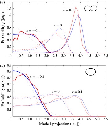
The difference in the p.d.f.s of ${\it\Omega}_{1}$ can be seen clearly in figure 5, where $p_{{\it\varepsilon}}({\it\omega}_{1})$ (blue curves) is plotted at three different values of the energy ( ${\it\varepsilon}=-0.1,~0,~0.1$ ) for domains A and B. Note that, since the p.d.f. is an even function of ${\it\omega}_{1}$ , it is plotted as a function of $|{\it\omega}_{1}|$ in figure 5 in order to facilitate comparison with the DNS (red curves, discussed in § 4.1 below). For reference, the (Gaussian) uniform ensemble p.d.f. is also plotted (dotted black curve).

Figure 6.

Contour plots comparing $p_{{\it\varepsilon}}(|{\it\omega}_{1}|,|{\it\omega}_{2}|)$ (a,b) predicted by the theory (3.16) with (c,d) statistics compiled from the DNS (2.2): (a,c) domain A; (b,d) domain B. The energy is fixed at ${\it\varepsilon}=0.05$ .

For any ordered set of $n$ integers $\{i_{1},i_{2},\ldots ,i_{n}\}$ the joint microcanonical p.d.f. $p_{{\it\varepsilon}}({\it\omega}_{i_{1}},{\it\omega}_{i_{2}},\ldots ,{\it\omega}_{i_{n}})$ of the random vector of vorticity projections $({\it\Omega}_{i_{1}},{\it\Omega}_{i_{2}},\ldots ,{\it\Omega}_{i_{n}})^{\text{T}}$ can also be calculated. The result is

(3.16) $$\begin{eqnarray}\displaystyle p_{{\it\varepsilon}}({\it\omega}_{i_{1}},{\it\omega}_{i_{2}},\ldots ,{\it\omega}_{i_{n}})=\frac{F^{{\bf\beta}(i_{1},i_{2},\ldots ,i_{n})}\left({\it\varepsilon}-{\it\varepsilon}_{0}+\displaystyle \mathop{\sum }_{i_{k}}{\displaystyle \frac{{\it\omega}_{i_{k}}^{2}-1}{2{\it\beta}_{i_{k}}}}\right)}{F^{{\bf\beta}}({\it\varepsilon}-{\it\varepsilon}_{0})}\,\frac{\text{exp}\left(-\displaystyle \mathop{\sum }_{i_{k}}{\displaystyle \frac{{\it\omega}_{i_{k}}^{2}}{2}}\right)}{(2{\rm\pi})^{n/2}}.\quad & & \displaystyle\end{eqnarray}$$

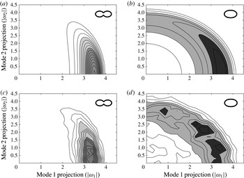
Of these joint p.d.f.s, the most interesting is arguably $p_{{\it\varepsilon}}({\it\omega}_{1},{\it\omega}_{2})$ because it illustrates the distribution of energy between the leading two normal modes of the system. Figure 6 contours $p_{{\it\varepsilon}}({\it\omega}_{1},{\it\omega}_{2})$ for domains A and B for energy ${\it\varepsilon}=0.05$ . The results show markedly different behaviours for the two domains. In domain A nearly all states have a significant amount of energy trapped in mode 1, whereas domain B allows energy to be shared comparatively efficiently between modes 1 and 2, evidenced by the circular pattern (only the upper right quadrant is shown) in figure 6. The difference can be explained by the difference in the spectral gap ${\it\beta}_{1}-{\it\beta}_{2}$ , between the two domains, as will be discussed further below.

3.3. The energy spectrum

For the 2D Euler equations in $\mathscr{D}$ , it is straightforward to define the ensemble-averaged fluid dynamical energy $E_{F}$ and the associated instantaneous discrete energy spectrum. Expanding the vorticity field ${\it\omega}(\boldsymbol{x})$ (here assumed to have zero mean) in the eigenfunctions $\{{\it\Phi}_{j}(\boldsymbol{x})\}$ as in (3.2) leads to

(3.17) $$\begin{eqnarray}E_{F}=-\frac{1}{2}\int _{\mathscr{D}^{2}}\langle {\it\omega}(\boldsymbol{x}){\it\omega}(\boldsymbol{x}^{\prime })\rangle G(\boldsymbol{x},\boldsymbol{x}^{\prime })\,\text{d}\boldsymbol{x}\,\text{d}\boldsymbol{x}^{\prime }={\it\omega}_{0}^{2}A^{2}\mathop{\sum }_{j=1}^{\infty }\langle E_{j}\rangle ,\quad \text{where}~E_{j}=-\frac{{\it\Omega}_{j}^{2}}{2{\it\beta}_{j}}\end{eqnarray}$$

and ${\it\Omega}_{j}=[{\it\omega}{\it\Phi}_{j}]/{\it\omega}_{0}$ as in (3.2). In general, ${\it\omega}_{0}$ is any scaling factor and the angle brackets denote an (unspecified) ensemble average. In the singular limit of the point vortex distribution (2.6), however, $E_{F}$ is undefined. Consequently, additional regularising terms are needed in the point vortex Hamiltonian (2.3); compare, for example, (3.6) and (3.17). Nevertheless, the fluid dynamical spectral coefficients $E_{j}$ in (3.17), which denote the energy in a mode with wavenumber $k_{j}=(-{\it\beta}_{j}/A)^{1/2}$ , do remain calculable in the point vortex system. In this case, ${\it\omega}_{0}=N^{1/2}{\it\Gamma}_{0}/A$ and the angle brackets unambiguously denote the microcanonical ensemble. In fact, it is demonstrated in appendix A that $\langle E_{j}\rangle$ has the following exact analytic relationship with the density-of-states function:

(3.18) $$\begin{eqnarray}\langle E_{j}\rangle =-\frac{1}{2{\it\beta}_{j}}\left(1+\frac{{\it\beta}({\it\varepsilon})}{{\it\beta}_{j}}-2\frac{{\it\beta}_{j}}{W({\it\varepsilon})}\frac{\partial W}{\partial {\it\beta}_{j}}({\it\varepsilon})\right).\end{eqnarray}$$

It is interesting to remark that the density-of-states function $W({\it\varepsilon})$ encodes, through (3.18), all information concerning the equilibrium point vortex energy spectrum (recall that ${\it\beta}({\it\varepsilon})=W^{\prime }({\it\varepsilon})/W({\it\varepsilon})$ ). An alternative expression (compare equation (38) of EAM13), which shows that it is not in fact necessary to evaluate the partial derivatives $\partial W/\partial {\it\beta}_{j}$ to obtain the energy spectrum from $W({\it\varepsilon})$ , is

(3.19) $$\begin{eqnarray}\langle E_{j}\rangle =\frac{1}{2W({\it\varepsilon})}\int _{-\infty }^{{\it\varepsilon}}W(\bar{{\it\varepsilon}})\,\text{e}^{{\it\beta}_{j}({\it\varepsilon}-\bar{{\it\varepsilon}})}\,\text{d}\bar{{\it\varepsilon}}.\end{eqnarray}$$

Equation (3.19) is obtained by integrating equation (A 8) given in appendix A.

Figure 7.

Point vortex energy spectra $\mathscr{E}(k)$ in domain B at different values of ${\it\varepsilon}$ .

In figure 7 the energy spectrum obtained from (3.18) is plotted for domain B for several values of ${\it\varepsilon}$ . The usual convention of summing the contributions from modes within wavenumber shells of finite width ${\rm\Delta}k$ is adopted. Here we take ${\rm\Delta}k=2\sqrt{{\rm\pi}}$ (consistent with taking ${\rm\Delta}k=1$ in the usual doubly periodic domain, which has greater area by a factor of $4{\rm\pi}$ ). Figure 7 shows that, as ${\it\varepsilon}$ is increased, energy is increasingly added to the largest scales in the system. At small scales the spectrum has a $k^{-1}$ slope for all values of ${\it\varepsilon}$ , consistent with the spectrum not being integrable. These results are consistent with spectra recently calculated numerically by Dritschel et al. (Reference Dritschel, Lucia and Poje2015) for the particular case of point vortices on the sphere. The dashed curve, showing the saturated spectrum, will be discussed below.

3.4. Large- ${\it\varepsilon}$ asymptotics, condensation and saturation spectrum

In appendix A it is proved that, as ${\it\varepsilon}\rightarrow \infty$ , the limiting density-of-states function satisfies

(3.20) $$\begin{eqnarray}W({\it\varepsilon})\approx \left(\frac{-{\it\beta}_{1}}{{\rm\pi}({\it\varepsilon}-{\it\varepsilon}_{0})}\right)^{1/2}\text{exp}\left({\it\beta}_{1}({\it\varepsilon}-{\it\varepsilon}_{0})-\frac{C_{1}}{2}-\mathop{\sum }_{k=1}^{\infty }{\displaystyle \frac{B_{k+1}}{k({\it\varepsilon}-{\it\varepsilon}_{0})^{k}}}\right),\end{eqnarray}$$

where $C_{1}$ is a constant,

(3.21) $$\begin{eqnarray}\displaystyle C_{1}=\mathop{\sum }_{j=2}^{\infty }\log \left(1-\frac{{\it\beta}_{1}}{{\it\beta}_{j}}\right)+\frac{{\it\beta}_{1}}{{\it\beta}_{j}}, & & \displaystyle\end{eqnarray}$$

and the $\{B_{k}\}$ are a sequence of negative constants also depending upon the eigenvalues $\{{\it\beta}_{j}\}$ (see table 1 in appendix A). Not only does (3.20) serve as a test of the numerical quadrature of (3.13), it also allows simplified analytical expressions to be obtained for various quantities of interest. The useful domain of validity of (3.20) can be estimated by inspection of figure 3(b,d), where the corresponding four-term approximation ${\it\beta}({\it\varepsilon})\approx \sum _{k=0}^{3}B_{k}({\it\varepsilon}-{\it\varepsilon}_{0})^{-k}$ (see table 1) is plotted (dashed green curves) against a quadrature of the exact expression (i.e. obtained from (3.13), solid green curves). Evidently the approximation is appropriate only for inverse temperatures below the critical value (i.e.  ${\it\beta}<{\it\beta}_{1}$ ), and works better in domain A than in domain B because the coefficients $\{B_{k}\}$ decay more rapidly in the former case.

Naturally, (3.20) also gives the $s\rightarrow \infty$ asymptotics of the functions $F^{\boldsymbol{w}}(s)$ of § 2.5. Hence, essentially the same asymptotics can be applied to the microcanonical p.d.f.  $p_{{\it\varepsilon}}({\it\omega}_{j})$ (given by (3.15)) of the vorticity projection ${\it\Omega}_{j}$ . It is found that, as ${\it\varepsilon}\rightarrow \infty$ , all but the first vorticity projection become normally distributed,

(3.22) $$\begin{eqnarray}{\it\Omega}_{j}\sim \mathscr{N}\left(0,\frac{{\it\beta}_{j}}{{\it\beta}_{j}-{\it\beta}_{1}}\right)\quad \text{for}~j\geqslant 2.\end{eqnarray}$$

Applying the method to (3.16) it can also be established that $\{{\it\Omega}_{2},{\it\Omega}_{3},\ldots \}$ become independent as ${\it\varepsilon}\rightarrow \infty$ . Interestingly, (3.22) is consistent with saturation of the fluid dynamical energy in each mode,

(3.23) $$\begin{eqnarray}\langle E_{j}\rangle =-\frac{\langle {\it\Omega}_{j}^{2}\rangle }{2{\it\beta}_{j}}\rightarrow \frac{1}{2({\it\beta}_{1}-{\it\beta}_{j})},\quad \text{as}~{\it\varepsilon}\rightarrow \infty ,\text{for}~j\geqslant 2.\end{eqnarray}$$

In other words, at large ${\it\varepsilon}$ , the energy spectrum of the point vortex system becomes saturated and, as ${\it\varepsilon}$ increases further, all of the additional energy must go into the condensate only. The saturated spectrum (3.23) is plotted on figure 7 (dashed curve). Note that, because $\langle E_{1}\rangle$ depends upon on the system energy ${\it\varepsilon}$ , the first energy shell is omitted. Spectral saturation is seen to be more or less complete by ${\it\varepsilon}=0.1$ , indicating that, as ${\it\varepsilon}$ increases beyond this value, all energy will go into the first energy shell (i.e. the condensate).

The p.d.f.  $p_{{\it\varepsilon}}({\it\omega}_{1})$ of the condensate vorticity projection ${\it\Omega}_{1}$ , by contrast, does not become Gaussian as ${\it\varepsilon}\rightarrow \infty$ . However, results about its behaviour can be found by taking the microcanonical ensemble average of (3.12), and using the results above. For example, the ensemble average of the condensate energy $E_{1}$ is found to be

(3.24) $$\begin{eqnarray}\langle E_{1}\rangle ={\it\varepsilon}-{\it\varepsilon}_{0}^{\ast },\quad {\it\varepsilon}_{0}^{\ast }={\it\varepsilon}_{0}+\frac{1}{2{\it\beta}_{1}}+\displaystyle \mathop{\sum }_{j=2}^{\infty }\frac{{\it\beta}_{1}}{2{\it\beta}_{j}({\it\beta}_{1}-{\it\beta}_{j})}.\end{eqnarray}$$

The domain-dependent constant ${\it\varepsilon}_{0}^{\ast }$ represents a correction to the mean-field theory to be discussed in the next subsection. Similarly, the variance of the condensate energy about its mean value is found to be

(3.25) $$\begin{eqnarray}\langle (E_{1}-\langle E_{1}\rangle )^{2}\rangle =\frac{1}{4}\mathop{\sum }_{j=2}^{\infty }\frac{1}{({\it\beta}_{1}-{\it\beta}_{j})^{2}},\end{eqnarray}$$

showing that the amplitude of fluctuations of the condensate energy are independent of ${\it\varepsilon}$ as ${\it\varepsilon}\rightarrow \infty$ . The predicted variance in (3.25) varies greatly between domains, e.g.  $\langle (E_{1}-\langle E_{1}\rangle )^{2}\rangle \approx 7.2\times 10^{-4}$ in domain A versus $2.4\times 10^{-2}$ in domain B, with the large difference explained by the clustering of the first few eigenvalues close to ${\it\beta}_{1}$ in domain B.

Figures 4–6 suggest that, as energy increases, switches in the sign of ${\it\Omega}_{1}$ will become increasingly infrequent in the dynamics, as the probability $p_{{\it\varepsilon}}({\it\omega}_{1}=0)$ of encountering a transition state with ${\it\Omega}_{1}=0$ becomes increasingly small. One might in fact anticipate that the expected time of transition is inversely proportional to $p_{{\it\varepsilon}}({\it\omega}_{1}=0)$ . This is in fact the case with stochastic models of bistable systems (e.g. Naso et al. Reference Naso, Chavanis and Dubrulle2010), which might be used as a simple phenomenological model for the dynamic evolution of ${\it\Omega}_{1}(t)$ here (see e.g. Touchette Reference Touchette2009, § 6.2). This idea will be explored in more detail in future work. In the large- ${\it\varepsilon}$ limit,

(3.26) $$\begin{eqnarray}p_{{\it\varepsilon}}({\it\omega}_{1}=0)\approx \left(\frac{{\it\beta}_{2}}{{\it\beta}_{1}}\right)^{1/2}\exp \left(-({\it\beta}_{1}-{\it\beta}_{2})({\it\varepsilon}-{\it\varepsilon}_{0})+\frac{C_{1}-C_{2}}{2}-\frac{{\it\beta}_{2}}{2{\it\beta}_{1}}\right),\end{eqnarray}$$

where $C_{2}$ is defined exactly as $C_{1}$ above, but with ${\it\beta}_{2}$ replacing ${\it\beta}_{1}$ and the sum starting at $j=3$ . The result (3.26) shows that the frequency of switches in the sign of ${\it\Omega}_{1}$ is highly sensitive to the spectral gap ${\it\beta}_{1}-{\it\beta}_{2}>0$ . In domain A, ${\it\beta}_{1}-{\it\beta}_{2}\approx 33.78$ , whereas in domain B, ${\it\beta}_{1}-{\it\beta}_{2}\approx 3.54$ , which explains the huge difference in switching behaviour between the two domains. The important point is that it is the shape of the domain that controls the spectral gap, and through this the switching frequency at high energy.

3.5. The connection with mean-field theory (sinh–Poisson equation)

Many researchers will be more familiar with the mean-field statistical mechanics theory of Joyce & Montgomery (Reference Joyce and Montgomery1973) than with the fluctuation theory considered above. What is the connection between the two theories? To answer this question, we will briefly review the mean-field theory for a uniform neutral gas below, and show how the main predictions relate to those of the fluctuation theory. The essential starting point is to recognise that, while the results of the fluctuation theory are expressed as a function of the scaled (thermodynamic) energy ${\it\varepsilon}=E/(N{\it\Gamma}_{0}^{2})$ , the mean-field results are expressed as a function of $e=E/(N^{2}{\it\Gamma}_{0}^{2})$ (sometimes referred to as the hydrodynamic energy). The fact that the energy scales differently with the number of vortices $N$ in each theory ( ${\it\varepsilon}=Ne$ ) means that, with respect to the density-of-states function in figure 1, the fluctuation theory is a theory of the central region, whereas the mean-field theory is a theory of the (positive) tail region. Pushing an analogy with sums of random variables in elementary statistics, it might be said that the fluctuation theory is the ‘central limit theorem’ for point vortices, with the mean-field theory acting as a ‘large-deviation theory’. According to this analogy, the two theories will be linked asymptotically, with the ${\it\varepsilon}\rightarrow \infty$ limit of the fluctuation theory matching to the $e\rightarrow 0$ limit of the mean-field theory (Pointin & Lundgren Reference Pointin and Lundgren1976).

The mean-field theory is formulated on the basis that the hydrodynamic energy $e$ of the system is positive, that all of this energy is contained in a steady mean flow (the condensate) and that fluctuations can be neglected. For the case of a uniform neutral gas, the mean-field theory leads to the well-known sinh–Poisson equation (Joyce & Montgomery Reference Joyce and Montgomery1973) for the time-mean streamfunction ${\it\psi}$ (scaled so that ${\rm\nabla}^{2}{\it\psi}=\langle {\it\omega}\rangle /N{\it\Gamma}_{0}$ ) of the condensate,

(3.27) $$\begin{eqnarray}\displaystyle {\rm\nabla}^{2}{\it\psi}=C\sinh ({\it\beta}_{h}{\it\psi}),\quad \text{where}~C=\frac{1}{A}\,[\exp ({\it\beta}_{h}{\it\psi})]^{-1/2}[\exp (-{\it\beta}_{h}{\it\psi})]^{-1/2}, & & \displaystyle\end{eqnarray}$$

where as above $[\cdot ]$ denotes the domain average. The correct boundary condition for ${\it\psi}$ on $\partial \mathscr{D}$ is (2.12). This can be seen, for example, by following the derivation of Pointin & Lundgren (Reference Pointin and Lundgren1976) – see discussion surrounding their equation (23). We note in passing that the Dirichlet condition ( ${\it\psi}=0$ on $\partial \mathscr{D}$ ) has occasionally been erroneously used in previous works, following, for example, Book, Fisher & McDonald (Reference Book, Fisher and McDonald1975). That (2.12) physically makes sense is clear: ${\it\psi}=\text{const.}$ on $\partial \mathscr{D}$ is sufficient to satisfy no normal flow, and the circulation condition on ${\it\psi}$ in (2.12) must hold from Green’s theorem in the plane, because the domain integral of the mean-field vorticity ${\rm\nabla}^{2}{\it\psi}$ is zero for a neutral gas. Consider also that (3.27) is not invariant under the transformation ${\it\psi}\rightarrow {\it\psi}+\text{const.}$ , and therefore specifying a value for ${\it\psi}$ on the boundary by using the Dirichlet boundary condition is evidently over-prescriptive. The inverse temperature ${\it\beta}_{h}={\it\beta}_{h}(e)$ appearing in (3.27) is determined from the mean-field energy

(3.28) $$\begin{eqnarray}e=-\frac{1}{2}\int _{\mathscr{D}}{\it\psi}{\rm\nabla}^{2}{\it\psi}\,\text{d}\boldsymbol{x}.\end{eqnarray}$$

It has been proved (Kiessling Reference Kiessling1995) that ${\it\beta}_{h}(e)$ is strictly negative. As discussed above, however, it is clear that both positive and negative temperatures exist in the point vortex system. At the outset it is thus clear that the mean-field theory is restricted to a limited range of  ${\it\beta}$ .

Asymptotic matching with the fluctuation theory requires that the system (3.27)–(3.28) be studied in the limit $E\rightarrow 0$ . In this limit (3.27) can be linearised to recover the eigenvalue problem (2.11). In other words, at low energies, distinct solutions of the sinh–Poisson equation emerge from $(e,{\it\beta}_{h})=(0,{\it\beta}_{1}),(0,{\it\beta}_{2}),\ldots \,$ . The mean-field theory can be used to show (Chavanis & Sommeria Reference Chavanis and Sommeria1996; Taylor et al. Reference Taylor, Borchardt and Helander2009) that, of these solutions, the first has maximum entropy and will therefore be selected by the dynamics. In the $E\rightarrow 0$ limit the first solution has streamfunction

(3.29) $$\begin{eqnarray}{\it\psi}(\boldsymbol{x})=\pm \left(-\frac{2e}{{\it\beta}_{1}}\right)^{1/2}{\it\Phi}_{1}(\boldsymbol{x}).\end{eqnarray}$$

Further, Taylor et al. (Reference Taylor, Borchardt and Helander2009) have shown that the caloric curve ${\it\beta}_{h}(e)$ associated with this first solution has expansion

(3.30) $$\begin{eqnarray}{\it\beta}_{h}(e)={\it\beta}_{1}-{\it\beta}_{1}^{2}\left(1-{\textstyle \frac{1}{3}}[{\it\Phi}_{1}^{4}]\right)e+O(e^{2}).\end{eqnarray}$$

Numerical solutions of (3.27)–(3.28) have been obtained, using the algorithm of McDonald (Reference McDonald1974), in domains A and B for a range of energies starting close to $E=0$ . These solutions have been used to obtain numerical estimates of ${\it\beta}_{h}(e)$ for each domain, and these have been plotted on figure 3 (blue curves) for $N=50$ and $N=100$ vortices (note that the number of vortices $N$ affects the scaling of the ${\it\beta}_{h}(e)$ curve in figure 3 because the ordinate is ${\it\varepsilon}=Ne$ and not $e$ ). The shape of the ${\it\beta}_{h}(e)$ curves can be seen only in panels (b) and (d), which expand the region near ${\it\beta}_{1}$ . For domain B, solutions emerging from both $(0,{\it\beta}_{1})$ and $(0,{\it\beta}_{2})$ (dotted line) are plotted. The corresponding small- $e$ approximation (3.30) has also been calculated and plotted (dashed blue line).

The results above allow us to consider matching between the ${\it\varepsilon}\rightarrow \infty$ limit of the fluctuation theory and the $e\rightarrow 0$ limit of the mean-field theory. First note that it is proved above, and is clear from figure 3, that both $\lim _{{\it\varepsilon}\rightarrow \infty }{\it\beta}({\it\varepsilon})={\it\beta}_{1}$ and $\lim _{e\rightarrow 0}{\it\beta}_{h}(e)={\it\beta}_{1}$ . Hence ${\it\beta}_{c}={\it\beta}_{1}$ is not only the critical inverse temperature for condensation, but is also the critical value for matching between the theories. Therefore, as $E$ is increased at finite $N$ , a smooth transition between the behaviour predicted by each theory can be expected for ${\it\beta}$ near ${\it\beta}_{c}$ . This transition will be examined numerically in § 4.2 below using phase-space sampling. Second, the solution (3.29) is consistent with the ${\it\varepsilon}\rightarrow \infty$ prediction for the fluctuation theory, because in the fluctuation theory all of the excess energy ends up in the condensate. The results (3.24)–(3.25) go beyond the mean-field theory result (3.29) by calculating the size of both the leading correction to the mean energy of the condensate and the variance of the condensate energy about this mean. The vorticity projection predicted by (3.29) is plotted on figure 4 as a blue dashed parabola, and shows that mean-field theory slightly underestimates the magnitude of the vorticity projections.

4.1. Direct numerical simulation

The ergodic hypothesis motivating the study of the microcanonical ensemble in § 3.2 is that the statistics of the microcanonical ensemble will correspond to the (long) time-averaged statistics of the equations of motion (2.2). This hypothesis will be tested next using DNS of (2.2). In particular, marginal p.d.f.s $p_{{\it\varepsilon}}({\it\omega}_{j})$ for the scaled vorticity projections $\{{\it\Omega}_{j}\}$ can be compared directly with statistics from the DNS. Here we will focus on $p_{{\it\varepsilon}}({\it\omega}_{1})$ , given by (3.15) and plotted in figure 5, as well as the joint p.d.f.  $p_{{\it\varepsilon}}({\it\omega}_{1},{\it\omega}_{2})$ contoured in figure 6.

DNS of equation (2.2) is performed using the adaptive algorithm described in Ashbee, Esler & McDonald (Reference Ashbee, Esler and McDonald2013). The majority of the runs to be discussed have been documented previously in EAM13. Briefly, (2.2) is solved for a uniform neutral gas with $N=100$ , in domains A and B, at a range of energies ( ${\it\varepsilon}=-0.15,~-0.1,~-0.05,~0,~0.05,~0.1,~0.15$ ) spanning the central region of the density-of-states function shown in figure 1. For each energy level and both domains, eight runs of $1000{\it\Gamma}_{0}^{-1}$ time units are executed, during which the evolving vorticity projections ${\it\Omega}_{j}(t)$ are calculated and recorded at regular time intervals ( $10{\it\Gamma}_{0}^{-1}$ ). Long time-averaged p.d.f.s are then compiled from the histograms of the recorded data.

The red curves in figure 5 show the DNS results for $p_{{\it\varepsilon}}(|{\it\omega}_{1}|)$ , which can be compared with the theoretical prediction (3.15) (blue curves). Notice that $p_{{\it\varepsilon}}(|{\it\omega}_{1}|)$ is plotted rather than $p_{{\it\varepsilon}}({\it\omega}_{1})$ . Here we are exploiting the fact that $p_{{\it\varepsilon}}({\it\omega}_{1})$ is an even function to aid comparison with the DNS. This is necessary because in the high-energy DNS (e.g.  ${\it\varepsilon}=0.1$ ), particularly in domain A, the system tends to become trapped for the duration of each run in a state with ${\it\Omega}_{1}$ either strictly positive or negative, producing asymmetric statistics. Good agreement is seen in figure 5, with much of the remaining discrepancy arguably due to the finite integration length over which our statistics were compiled. In particular, the large contrast in the shape of $p_{{\it\varepsilon}}(|{\it\omega}_{1}|)$ between the two domains is equally apparent in the DNS as it is in the theory. Similarly, the DNS results in figure 6(c,d) agree well with the theoretical prediction of (3.16) (figure 6 a,b). The contrast between the two domains is again equally apparent in the DNS.

A further testable prediction is that the time-mean streamfunction $\langle {\it\psi}\rangle$ in the DNS, at energies in the matching region (low $e$ , high ${\it\varepsilon}$ ), is at leading order given by (3.29). In particular, the spatial structure of the condensate should match that of the first non-constant eigenfunction ${\it\Phi}_{1}(\boldsymbol{x})$ . Domains C and D have been selected to provide an exacting numerical test that the correct spatial structure of $\langle {\it\psi}\rangle$ emerges, because, as shown in figure 2, the two geometrically similar domains have very different first eigenfunctions. In domain C, ${\it\Phi}_{1}(\boldsymbol{x})$ has a tripole structure dominated by a single large vortex in the centre of the domain, whereas in domain D ${\it\Phi}_{1}(\boldsymbol{x})$ has a left–right dipole structure.

The numerical runs for domains C and D are initialised with $N=100$ randomly placed vortices, and are executed just as described above for domains A and B, but for a longer duration ( $3000{\it\Gamma}_{0}^{-1}$ time units) and at higher energy ( ${\it\varepsilon}=1.3$ for C and ${\it\varepsilon}=1.1$ for D). High energy is necessary to prevent switches in the polarity of the circulation, as described above, occurring during the DNS. During each run, the exact instantaneous streamfunction at every point on a spatial grid is recorded. Note that, although the instantaneous streamfunction has logarithmic singularities at the locations of the vortices, provided that a vortex location is never exactly coincident with a grid point, the time average at the grid point remains well defined. Moreover, owing to the gentle nature of the logarithmic singularity, ‘near-misses’ where vortices pass close to grid points do not dominate the time average.

Figure 8.

(a,c) Time-mean streamfunction (scaled by $N{\it\Gamma}_{0}$ as in § 3.5) $\langle {\it\psi}(\boldsymbol{x})\rangle$ , calculated for time interval $1000{\it\Gamma}_{0}^{-1}<t<3000{\it\Gamma}_{0}^{-1}$ , for dynamical runs with $N=100$ vortices in domains C and D. The energies are (C) $e=E/N^{2}{\it\Gamma}_{0}^{2}=0.013$ ( ${\it\varepsilon}=1.3$ ) and (D)  $e=0.011$ ( ${\it\varepsilon}=1.1$ ). (b,d) Linearised sinh–Poisson solution $(-2e/{\it\beta}_{1})^{1/2}{\it\Phi}_{1}(\boldsymbol{x})$ for the two domains. Contour intervals are the same in each panel.

Figure 8 shows a comparison between the time-mean streamfunction $\langle {\it\psi}\rangle$ calculated from the DNS (a,c) and the theoretical predictions (b,d). The DNS results capture the contrasting structures between the two domains. The $N=100$ vortex runs have been repeated with many sets of randomly generated initial conditions across a range of similar energies, and the emergence of the distinct structures in $\langle {\it\psi}\rangle$ in each domain has been found to be very robust. A detailed numerical investigation of the ‘geometry-controlled transition’ (see also Chavanis & Sommeria Reference Chavanis and Sommeria1996; Taylor et al. Reference Taylor, Borchardt and Helander2009) between the two structures, as the domain shape is varied smoothly between domains C and D, is presented in Ashbee (Reference Ashbee2014).

4.2. Phase-space sampling using a multi-canonical Markov chain Monte Carlo (MC3) method

The results of § 3 can also be validated against statistics generated from repeatedly sampling the uniform distribution (see e.g. Campbell & O’Neil Reference Campbell and O’Neil1991; Bühler Reference Bühler2002; Esler et al. Reference Esler, Ashbee and McDonald2013; Billam et al. Reference Billam, Reeves, Anderson and Bradley2014). In the naive approach, the $N$ vortices are randomly distributed in the domain with uniform measure, and quantities of interest such as the energy and the vorticity projections ${\it\Omega}_{j}$ are calculated for the distribution in question and recorded. Repeating the process allows histograms to be generated from the recorded data, which then serve as estimates of the probability densities $p_{0}(\cdot )$ under the uniform ensemble. Probability densities under the microcanonical ensemble $p_{{\it\varepsilon}}(\cdot )$ can be generated from subsets of the data for which the energy lies in a shell centred on the energy  ${\it\varepsilon}$ of interest.

If the point vortex system is ergodic, p.d.f.s obtained by sampling the microcanonical canonical ensemble and p.d.f.s obtained from long-time integrations of the dynamics (2.2) should be identical to within statistical error. For our calculations with $N=100$ , this is indeed what we have found, i.e. there is no evidence of non-ergodicity, in contrast to the $N=6$ doubly periodic calculations reported by Weiss & McWilliams (Reference Weiss and McWilliams1991).

The main drawback with the naive sampling method described above is that it is very expensive to generate data outside the central region of the density-of-states function illustrated in figure 1 (i.e. outside $-0.2\lesssim {\it\varepsilon}\lesssim 0.3$ ), simply because the vast majority of random distributions of vortices will have energy within that range. To bypass the need to sample all energy levels simultaneously, and as a method of investigating energy levels outside of the central region, methods of sampling constant energy surfaces have been developed (Creutz Reference Creutz1983). Creutz’s method has been used with apparent success in the point vortex context by Smith (Reference Smith1989) but has the disadvantages that (i) no proof exists that the microcanonical ensemble is accurately represented, and (ii) it does not allow direct calculation of the inverse temperature ${\it\beta}$ for comparison with theory.

An alternative method is multi-canonical Markov chain Monte Carlo (MC3) sampling (Berg Reference Berg2000; Driscoll & Maki Reference Driscoll and Maki2007). In its simplest form, MC3 can be regarded as a method for sampling the tail regions of one-dimensional p.d.f.s, and in our set-up the p.d.f. in question is the density-of-states function $W_{{\it\bf\Gamma}}(E)$ . Our implementation of the MC3 algorithm closely follows the structure of the MATLAB code published by Driscoll & Maki (Reference Driscoll and Maki2007) – see discussion surrounding their figure 4 – used therein to estimate the (known) binomial p.d.f. of a one-dimensional random walk. For our problem, a Markov chain is initialised with a random distribution of vortices, and is updated at each step by moving a single vortex, chosen at random, to a new random position in $\mathscr{D}$ . The algorithm proceeds, for states in the positive tail region of $W_{{\it\bf\Gamma}}(E)$ , by accepting an update if the new distribution of vortices has greater energy $E$ , and rejecting it with a certain probability if the updated $E$ is lower. The MC3 algorithm then uses the accumulated statistics of how $E$ changes under updates to adjust the rejection probabilities. The result is that, after a sufficient number of iterations, $W_{{\it\bf\Gamma}}(E)$ is sampled with optimal efficiency far into the tail regions with an unbiased method.

MC3 has been used to sample $W_{{\it\bf\Gamma}}(E)$ in domains A and B, where the circulations ${\it\bf\Gamma}$ are those of a uniform neutral gas with $N=100$ . A Markov chain length of $1.5\times 10^{7}$ was used for each iteration, of which the first third is a ‘burn-in’, which is not used when compiling the statistics. Note that the fact that only one vortex is moved each time the chain is advanced can be used to accelerate the calculation of the energy and vorticity projections, allowing for efficient calculation of long chains. Twenty iterations were found to be necessary for the statistics to converge on the energy interval $-0.2\lesssim {\it\varepsilon}\lesssim 2.5$ . The failure of MC3 to significantly extend the statistics in the negative energy tail is due to the double exponential decay of $W_{{\it\bf\Gamma}}(E)$ as $E\rightarrow -\infty$ (see figure 1).

Numerical differentiation was then used to obtain the corresponding inverse temperatures ${\it\beta}_{{\it\bf\Gamma}}(E)=W_{{\it\bf\Gamma}}^{\prime }(E)/W_{{\it\bf\Gamma}}(E)$ , which are plotted in figure 3 (red curves, $N{\it\Gamma}_{0}^{2}{\it\beta}_{{\it\bf\Gamma}}$ plotted as a function of ${\it\varepsilon}=E/N{\it\Gamma}_{0}^{2}$ ). The calculated inverse temperatures can be compared with the theoretical predictions ${\it\beta}({\it\varepsilon})$ (fluctuation theory, green curves) and ${\it\beta}_{h}(e)$ (mean-field theory, blue curves). Figure 3(a,c) cover the central region $(-0.2<{\it\varepsilon}<0.3)$ , which could equally well have been sampled using the naive method, and show excellent agreement between the MC3 sampled ${\it\beta}_{{\it\bf\Gamma}}(E)$ and the fluctuation theory ${\it\beta}({\it\varepsilon})$ . Figure 3(b,d), by contrast, focus on the positive tail region $(0\lesssim {\it\varepsilon}<2)$ and show inverse temperatures close to the critical value ${\it\beta}={\it\beta}_{1}$ (dashed line). On this scale, the MC3 results show a remarkable transition between close agreement with the fluctuation theory at lower energies, and close agreement with mean-field theory prediction ${\it\beta}_{h}(e)$ at higher energies. Accurate statistical validation of ${\it\beta}_{h}(e)$ , which has not (to the authors’ knowledge) been attempted previously, has therefore been made possible by MC3. The naive method is computationally too expensive by several orders of magnitude. To check the robustness of the result, the MC3 calculation was repeated for domain A with $N=50$ vortices. Recall that, because figure 3 is plotted as a function of the thermodynamic energy ${\it\varepsilon}=E/N{\it\Gamma}_{0}^{2}$ rather than the hydrodynamic energy $e={\it\varepsilon}/N$ , the mean-field theory prediction ${\it\beta}_{h}(e)$ must be replotted on figure 3 when $N$ is changed. Nevertheless, the MC3 calculation (dark red curve) reveals that a clear transition between agreement with ${\it\beta}({\it\varepsilon})$ to agreement with ${\it\beta}_{h}(e)$ again takes place, i.e. both theories are correct within their range of validity.

Figure 9.

(a–c) The microcanonical p.d.f.  $p_{{\it\varepsilon}}({\it\omega}_{1})$ of the vorticity projection ${\it\Omega}_{1}$ at energy  ${\it\varepsilon}$ , calculated for domain A with a uniform neutral gas, contoured as a function of $({\it\omega}_{1},{\it\varepsilon})$ : (a) MC3 calculation with $N=20$ vortices; (b) MC3 with $N=50$ ; and (c) MC3 with $N=100$ . (d) The theoretical prediction (3.15).

Statistics compiled using MC3 can also be used as a check on the p.d.f.s of the vorticity projections. In figure 4(d–f), $p_{{\it\varepsilon}}({\it\omega}_{1})$ , as calculated from histograms compiled from the MC3 data with $N=100$ vortices, is contoured. Excellent agreement with the theoretical predictions of (3.15) is evident in all three domains (A, C, D). It is clear from figure 4 that $N=100$ vortices are sufficient for the theory to be accurate; hence an obvious question relates to how the theory performs as $N$ is decreased. Figure 9 compares $p_{{\it\varepsilon}}({\it\omega}_{1})$ estimated from MC3 calculations in domain A with $N=20,~50$ and $100$ vortices with the theoretical prediction. Even with as few as $N=20$ vortices, the phase transition between the uncondensed and condensed states is seen to occur at an almost identical energy ${\it\varepsilon}$ . At higher energies, there is a quantitative difference with the expected values of $|{\it\Omega}_{1}|$ somewhat lower for $N=20$ compared with the theory. An explanation for the difference is that ${\it\varepsilon}=0.7$ in figure 9 corresponds to a significantly higher value of the hydrodynamic energy $e$ at low $N$ ( $e=0.035$ for $N=20$ compared to $e=0.007$ for $N=100$ ). The former value of $e$ is sufficiently high for the sinh–Poisson equation (3.27) to predict significant nonlinearity in the $\langle {\it\omega}\rangle$ – $\langle {\it\psi}\rangle$ relationship, and an associated change in the spatial structure of $\langle {\it\psi}\rangle$ , causing it to differ significantly from that of ${\it\Phi}_{1}(\boldsymbol{x})$ .