1 Introduction
A slender body at incidence to a moving stream experiences a lift force, where this force is largely influenced by cross-flow separation in the form of wake vortices. There is a wealth of research literature on studies of inclined slender-body wakes given their relevance, for example, in the dynamic control and prediction of safe manoeuvre of airships and submarines. Some useful references to supplement reading include the works of Sarpkaya (Reference Sarpkaya1966) and Schindel (Reference Schindel1969) on vortex separation about lifting bodies, the measurement techniques discussed by Wetzel (Reference Wetzel1996) and Chesnakas & Simpson (Reference Chesnakas and Simpson1997) for detecting surface-flow separation lines, the use of topological concepts by Wang (Reference Wang1972), Tobak & Peake (Reference Tobak and Peake1982) and Lee (Reference Lee2015) to interpret cross-flow patterns and the use of high-resolution Reynolds-averaged Navier–Stokes computation by Jeans et al. (Reference Jeans, Watt, Gerber, Holloway and Baker2009) to obtain vorticity fields for force estimation. An insight into slender-body wakes also may be found in more recent literature. Examples include the high-Reynolds-number experiments by Ashok, Van Buren & Smits (Reference Ashok, Van Buren and Smits2015) which documented the persistence of natural asymmetry in wake vortices, and the direct numerical simulation of Jiang et al. (Reference Jiang, Andersson, Gallardo and Okulov2016) which presented data for testing of concepts of self-similarity in asymmetric wakes, where the wakes may be dominated by complex helical-like vortices.
Flow separation over a slender body (6:1 prolate spheroid at
 $\unicode[STIX]{x1D713}=20^{\circ }$
); the body-length Reynolds number
 $\mathit{Re}_{L}$
is (a)
 $4.2\times 10^{6}$
and (b)
 $6.5\times 10^{6}$
. After Wetzel, Simpson & Chesnakas (Reference Wetzel, Simpson and Chesnakas1998).

It is interesting, from laboratory observation and from the literature review, that the most apparent features of slender-body wakes are the surface-flow separation lines because these lines define the start of the wakes. An example of a slender body which has been extensively tested is that of a prolate spheroid (e.g. Chesnakas & Simpson Reference Chesnakas and Simpson1997; Wetzel et al.
Reference Wetzel, Simpson and Chesnakas1998). In figure 1(a), the cross-flow pattern constructed from laser-Doppler-velocimetry data and the skin-friction minima obtained from hot-film data show the separation lines (or negative surface bifurcations
 $B_{1}^{-}$
and
 $B_{2}^{-}$
) on this geometry, where these lines correspond to saddle points (
 $S_{1}$
and
 $S_{2}$
) of the wake flow. A detailed map of the skin-friction lines is given in figure 1(b), where the locations of separations are identified by the local minima of skin-friction magnitude (see Wetzel et al.
Reference Wetzel, Simpson and Chesnakas1998). Here, the wake flow contains a pair of counter-rotating primary and secondary vortices. In the half-symmetry plane shown in figure 1, the larger vortex is a sink focus (
 $F_{1}$
) produced by the primary separation (
 $B_{1}^{-}$
), and the smaller eddy is a source focus (
 $F_{2}$
) adjacent to the secondary separation (
 $B_{2}^{-}$
) to satisfy flow continuity. Since the wake flow starts from the separation lines, the off-body vortices generally move in the same longitudinal direction as the separation lines.
Figure 2(a) provides a schematic diagram of a generic slender body which consists of a rounded nose of length
 $l_{n}$
, a cylindrical midsection of length
 $l_{m}$
and a tapered tail of length
 $l_{t}$
. In the case of a prolate spheroid (e.g. figure 1), the nose and the tail are mirrored geometries of equal length (
 $l_{n}=l_{t}$
) and there is no cylindrical midsection.
Schematic diagram of a generic slender body: (a) component definitions and (b) cross-flow orientation. Dimensions for (c) test geometries G1, G2 and G3 are given in table 1.

For translational motion as shown in figure 2(b), Jeans & Holloway (Reference Jeans and Holloway2010) indicated that the development of separation lines over the body at incidence
 $\unicode[STIX]{x1D713}$
may be formulated as a transient problem which relates the longitudinal distance (
 $x$
measured from the nose) to time:
 $$\begin{eqnarray}t=\frac{x}{U_{\infty }\,\cos (\unicode[STIX]{x1D713})},\quad t_{r_{m}}^{\ast }=t\,\,\frac{U_{\infty }\,\sin (\unicode[STIX]{x1D713})}{r_{m}}=\frac{x}{r_{m}}\,\text{tan}(\unicode[STIX]{x1D713}),\end{eqnarray}$$
where
 $r_{m}$
is the maximum radius of the body, and
 $\text{tan}(\unicode[STIX]{x1D713})$
defines the ratio between the cross-flow and body-axis components of the free-stream velocity
 $U_{\infty }$
. The scaling (1.1) is based on an analogy by Sarpkaya (Reference Sarpkaya1966) and Schindel (Reference Schindel1969) which relates the development of cross-flow at each longitudinal station along the slender body to the development with time of the flow on an impulsively started two-dimensional cylinder. This analogy is derived from a National Advisory Committee for Aeronautics (NACA) vortex model described by Allen (Reference Allen1949), among others, for predicting lift.
In their study, Jeans & Holloway (Reference Jeans and Holloway2010) developed a model to scale the primary-separation angle (
 $\unicode[STIX]{x1D6E9}_{B_{1}^{-}}$
) as a function of
 $t_{r_{m}}^{\ast }$
, the non-dimensionalised time defined in (1.1), for a collection of different submarine hull forms with the aid of a Reynolds-averaged Navier–Stokes (RANS) simulation database. Their findings indicated that the length (or time) of the primary separation increases with the incidence angle
 $\unicode[STIX]{x1D713}$
, and that
 $\unicode[STIX]{x1D713}$
has a strong effect on the separation lines along the tapered tail (see component definitions in figure 2). Upstream of the tail, Jeans & Holloway (Reference Jeans and Holloway2010) observed that the primary-separation angle along the cylindrical midsection of a slender body approximately follows the exponential function:
 $$\begin{eqnarray}(\unicode[STIX]{x1D6E9}_{B_{1}^{-}}-\unicode[STIX]{x1D6E9}_{B_{1}^{-}}^{\infty })/(\unicode[STIX]{x1D6E9}_{B_{1}^{-}}^{o}-\unicode[STIX]{x1D6E9}_{B_{1}^{-}}^{\infty })\simeq \text{e}^{-k_{r_{m}}^{}\,\,t_{r_{m}}^{\ast }},\end{eqnarray}$$
where
 $\unicode[STIX]{x1D6E9}_{B_{1}^{-}}^{o}=180^{\circ }$
is chosen to correspond to the leeward side, and the steady-state separation angle
 $\unicode[STIX]{x1D6E9}_{B_{1}^{-}}^{\infty }\simeq 112^{\circ }$
and the exponent
 $k_{r_{m}}^{}\simeq 0.5$
are obtained empirically since it is difficult to determine exactly where separation first occurs. This is mainly because there are no sharp edges to fix the separation, and where separation first occurs it is likely dependent on the initial development over the slender body.
The aim of the work reported in the following pages is to obtain further understanding of the development of flow-separation lines on inclined slender bodies. The key parameters of interest include the body geometry and the incidence angle. Here, the separation lines are interpreted by using flow-visualisation data from present wind-tunnel experiments and by using high-Reynolds-number data from open literature.
2 Body geometry and experimental technique
Test geometries with body length
 $L=l_{n}+l_{m}+l_{t}$
and maximum radius
 $r_{m}$
as shown in figure 2.

This study makes use of an existing generic axisymmetric body which is available from the Aerospace Division of the Defence Science and Technology Group. The slender body of choice has a NACA0033 profile with the fineness ratio
 $R=L/(2r_{m})$
, where the nose and the tail can be split at the location of maximum radius
 $r_{m}$
so that a cylindrical midsection (of radius
 $r_{m}$
) can be introduced to increase the overall body length
 $L$
. Figure 2(c) shows the geometry with three different lengths
 $l_{m}$
of the midsection:
 $M=l_{m}/(2r_{m})=$
0, 1 and 3. For
 $M=0$
, this defines the NACA geometry with length
 $x/L\equiv x^{\prime }$
in the range
 $0\leqslant x^{\prime }\leqslant 1$
and the local body radius
 $r(x)/L\equiv r(x^{\prime })$
, where
 $$\begin{eqnarray}r(x^{\prime })=0.33(1.4845\sqrt{x^{\prime }}-0.6300x^{\prime }-1.7580(x^{\prime })^{2}+1.4215(x^{\prime })^{3}-0.5075(x^{\prime })^{4}).\end{eqnarray}$$
For
 $M>0$
, the details of the nose, the midsection and the tail are given below and in table 1.
(i) The NACA nose has the profile
(2.2a-c )with $$\begin{eqnarray}\left.\frac{x}{L}\right|_{n}=\frac{x^{\prime }}{0.33M+1},\quad \left.\frac{r(x)}{L}\right|_{n}=\frac{r(x^{\prime })}{0.33M+1},\quad \frac{l_{n}}{L}=\frac{0.3}{0.33M+1},\end{eqnarray}$$
$0\leqslant x^{\prime }\leqslant 0.3$
and
$0\leqslant x\leqslant l_{n}$
, where
$l_{n}$
is the length of the nose.
(ii) The cylindrical midsection has the proportions
(2.3a,b )with$$\begin{eqnarray}\left.\frac{r(x)}{L}\right|_{m}=\frac{r_{m}}{L}=\frac{0.33/2}{0.33M+1},\quad \frac{l_{m}}{L}=\frac{0.33M}{0.33M+1},\end{eqnarray}$$
$l_{n}<x\leqslant l_{n}+l_{m}$
, where
$l_{m}$
is the length of the midsection.(iii) The NACA tail has the profile
(2.4a-c )with$$\begin{eqnarray}\left.\frac{x}{L}\right|_{t}=\frac{0.33M+x^{\prime }}{0.33M+1},\quad \left.\frac{r(x)}{L}\right|_{t}=\frac{r(x^{\prime })}{0.33M+1},\quad \frac{l_{t}}{L}=\frac{L-(l_{n}+l_{m})}{L}=\frac{0.7}{0.33M+1},\end{eqnarray}$$
$0.3<x^{\prime }\leqslant 1$
and
$l_{n}+l_{m}<x\leqslant l_{n}+l_{m}+l_{t}$
, where
$l_{t}$
is the length of the tail. To allow sting mounting for wind-tunnel testing, the tail is truncated at the longitudinal location (see table 1): (2.5)$$\begin{eqnarray}\frac{x_{s}}{L}=\frac{0.33M+0.85}{0.33M+1}.\end{eqnarray}$$






The slender body has a fixed maximum radius
 $r_{m}=64~\text{mm}$
; it is made of aluminium and is painted black for testing in the DST low-speed wind tunnel. The wind-tunnel test section has width 2.7 m, height 2.1 m and length 6.6 m (e.g. Erm Reference Erm2003). The free stream is operated at
 $U_{\infty }=85~\text{m}~\text{s}^{-1}$
,
 $64~\text{m}~\text{s}^{-1}$
and
 $42~\text{m}~\text{s}^{-1}$
for the respective geometries G1, G2 and G3 to yield the same body-length Reynolds number
 $\mathit{Re}_{L}=LU_{\infty }/\unicode[STIX]{x1D708}=2.1\times 10^{6}$
, where
 $\unicode[STIX]{x1D708}$
is the kinematic viscosity of the working fluid (i.e. air). To trip the flow, a circumferential ring of fine carborundum particles (of size
 $100~\unicode[STIX]{x03BC}\text{m}$
) is fixed at 15 % of the body length
 $L$
.
The body is attached to a sting and is remote controlled by a sting-column rig which allows pitch (
 $0^{\circ }\leqslant \unicode[STIX]{x1D713}<40^{\circ }$
), roll and vertical traverse. To visualise the surface flow, a paint mixture of white China-clay powder (
 ${\sim}$
9 % by volume), kerosene (
 ${\sim}$
90 %) and oleic acid (
 ${\sim}$
1 %) is used for this experiment. Trial and error indicated that the best results are obtained by painting the body just outside the test section (above a rectangular open slot in the test-section ceiling) and immediately traversing the body down to a set point in the test section at the required pitch while the wind tunnel is running at the correct flow speed. This process helps to avoid spurious flow patterns produced by (i) the initial ramp-up of the tunnel speed, and (ii) the gravitational effect on the paint mixture.
Once the flow pattern has settled with the kerosene evaporated (which takes a few minutes), the dried China clay provides a strong contrast against the black body to allow still photography. A
 $360^{\circ }$
view is obtained with a fixed position of the camera as the rig rolls the body about its longitudinal axis. Images of the flow pattern are recorded for each pitch or incidence angle
 $\unicode[STIX]{x1D713}=20,25,30$
and
 $35^{\circ }$
. The present test omitted angles
 $\unicode[STIX]{x1D713}\leqslant 15^{\circ }$
because the separation lines at these angles occur much further aft and are affected by flow stagnation at the sting junction; also they are more difficult to measure due to smaller spatial dimension of the tapered tail.
China-clay images and surface streaklines for geometry G1;
 $\unicode[STIX]{x1D713}=35^{\circ }$
;
 $\mathit{Re}_{L}=2.1\times 10^{6}$
.

3 Flow topology of the slender body
Figure 3 shows examples of recorded China-clay images for the geometry G1. The other geometries G2 and G3 produce very similar surface-flow patterns. The major features (as shown in figure 3) are interpreted as follows.
(i) The source node
$N_{1}$
– this is due to flow stagnation on the windward side of the nose.(ii) The positive bifurcations
$B_{1}^{+}$
and
$B_{2}^{+}$
– they define on the slender body the bottom and top symmetry lines which extend from the source node to the truncated tail.(iii) The negative bifurcations
$B_{1}^{-}$
and
$B_{2}^{-}$
– they represent regions of concentrated surface streaklines. The flow spreading circumferentially from the bottom (windward side;
$\unicode[STIX]{x1D6E9}=0^{\circ }$
) and the top (leeward side;
$\unicode[STIX]{x1D6E9}=180^{\circ }$
) of the body converges here to satisfy flow continuity. The negative bifurcation closest to the windward side is the primary line (
$\unicode[STIX]{x1D6E9}_{B_{1}^{-}}$
) and the negative bifurcation closest to the leeward side is the secondary line (
$\unicode[STIX]{x1D6E9}_{B_{2}^{-}}$
). The separation angles fall in the range
$0^{\circ }<\unicode[STIX]{x1D6E9}_{B_{1}^{-}}<\unicode[STIX]{x1D6E9}_{B_{2}^{-}}<180^{\circ }$
.



In figure 3, the surface streaklines are visually traced from the China-clay images (using the ‘Xfig’ graphics software) to identify the separation locations. To obtain discrete measurements from each geometry, the streakline pattern is divided into 20 longitudinal segments at increments
 $x/L=0.05$
with 72 azimuthal segments at increments
 $\unicode[STIX]{x1D6E9}=5^{\circ }$
and assigning the locations of the separations (
 $\unicode[STIX]{x1D6E9}_{B_{1}^{-}}$
and
 $\unicode[STIX]{x1D6E9}_{B_{2}^{-}}$
) to the nearest segments. The size of the selected grid in the azimuthal
 $\unicode[STIX]{x1D6E9}$
direction is the approximate minimum in which the separation locations can be resolved visually (with a measurement uncertainty
 $\unicode[STIX]{x1D6FF}_{\unicode[STIX]{x1D6E9}}\simeq \pm 5^{\circ }$
). For each geometry at a given incidence angle, the pattern is folded about the symmetry plane to reduce possible scatter, and the results are summarised as a collection of discrete data points in figure 4.
Given that the slender body is truncated to blend into a cylindrical sting, figure 3 shows that the separation lines can stagnate at this junction and terminate as a pair of sink foci and saddle points. In figure 4, the measurements are taken sufficiently upstream of the truncation to avoid possible effect of stagnation due to the sting–body junction. If the slender body is not truncated and if there is no sting interference, then the simplest possible flow pattern is that which all streaklines originate from a source node on the nose and eventually terminate at a sink node on the tail to satisfy the closed-surface topology, that is, number of nodes
 $-$
number of saddles
 $=2$
(e.g. Wang Reference Wang1972; Tobak & Peake Reference Tobak and Peake1982; Lee Reference Lee2015).
Separation lines on geometries (a) G1, (b) G2 and (c) G3;
 $\mathit{Re}_{L}=2.1\times 10^{6}$
.

4 Separation lines of the surface flow
Inspection of the flow topology in figure 3 and dimensional analysis of the data in figure 4 suggest that the azimuthal location of separation,
 $\unicode[STIX]{x1D6E9}$
, may be expressed as a function of longitudinal development time and the body-length Reynolds number,
 $$\begin{eqnarray}\unicode[STIX]{x1D6E9}=\boldsymbol{f}(t^{\ast },\mathit{Re}_{L}),\end{eqnarray}$$
where
 $t^{\ast }$
is a generalised form of the time scale (1.1) which relates to the local body radius
 $r(x)$
and the incidence angle
 $\unicode[STIX]{x1D713}$
, viz.
 $$\begin{eqnarray}t^{\ast }=t_{r_{m}}^{\ast }\,\frac{r_{m}}{r(x)}=\frac{x}{r(x)}\,\text{tan}(\unicode[STIX]{x1D713}).\end{eqnarray}$$
4.1 On the time scale
A plot of the data from figure 4 as a function of (1.1) in figure 5 shows the effect of the tapered tail on the flow separation, where an increase in
 $\unicode[STIX]{x1D713}$
increases the characteristic time
 $t_{r_{m}}^{\ast }$
of the separation lines. To account for the different trends in separation along the tail, the data points are replotted in figure 6, where
 $t_{r_{m}}^{\ast }$
is weighted by the ratio
 $r_{m}/r(x)$
as defined in (4.2). Figure 6 shows that the
 $t^{\ast }$
scaling yields a collapse of all the data points; a slight scatter may be due to (i) the uncertainty in the visual inspection
 $\unicode[STIX]{x1D6FF}_{\unicode[STIX]{x1D703}}\simeq \pm 5^{\circ }$
, and/or (ii) the strong turbulence of the separating flow since the splitting of the NACA geometry (G1) to include a long cylindrical midsection (G2, G3) makes the geometry less streamlined.
Separation lines as functions of
 $t_{r_{m}}^{\ast }$
for (a) G1, (b) G2 and (c) G3;
 $\mathit{Re}_{L}=2.1\times 10^{6}$
.

Inspection of figure 6 suggests that the locus of separation (
 $l$
) may be approximated by a power law of
 $t^{\ast }$
, viz.
 $$\begin{eqnarray}\unicode[STIX]{x1D6E9}_{B_{l}^{-}}\sim (t^{\ast })^{k_{l}},\quad t^{\ast }\geqslant t_{s}^{\ast },\quad l=1,2,\end{eqnarray}$$
where
 $t_{s}^{\ast }$
is the start time for the power law and
 $k$
is the separation rate. Given that there is little discernible difference between the separation trends in figure 6, the data points for geometries G1, G2 and G3 are combined in figure 7(a) to provide an estimate of
 $k$
. In figure 7(a), the root-mean-square (r.m.s.) difference between the power law and the combined data for the primary line is 3.5 % with
 $k_{1}=-0.223$
, and for the secondary line the r.m.s. difference is 1.8 % with
 $k_{2}=0.033$
. For the power-law curve fits shown in figure 7(a), the start time is at
 $t_{s}^{\ast }=1.42$
.
4.2 On the Reynolds number
In figure 7(a), the time scale
 $t^{\ast }$
provides a collapse of all the data points for the different geometries (G1, G2 and G3) tested in the range
 $20^{\circ }\leqslant \unicode[STIX]{x1D713}\leqslant 35^{\circ }$
at a fixed body-length Reynolds number
 $\mathit{Re}_{L}=2.1\times 10^{6}$
. The collapsed data are well represented by a power law,
 $\unicode[STIX]{x1D6E9}\sim (t^{\ast })^{k}$
, and so the exponent
 $k$
can be used as a measure of separation rate.
Separation lines as functions of
 $t^{\ast }$
for (a) G1, (b) G2 and (c) G3;
 $\mathit{Re}_{L}=2.1\times 10^{6}$
.

Present study of separation lines on slender bodies. (a) All data points taken from figure 6;
 $\mathit{Re}_{L}=2.1\times 10^{6}$
. (b) Supplementary China-clay data from a NACA0018-nose-cylinder;
 $\mathit{Re}_{L}=8\times 10^{6}$
. The solid curves show the separations modelled by (4.3) with a
 $\pm 5^{\circ }$
departure indicated by the shaded regions.

To investigate the effect of increasing body-length Reynolds number (
 $\mathit{Re}_{L}$
) on the separation rate
 $k$
defined by (4.3), a larger slender body of fineness ratio
 $R=10.0$
has been constructed for testing in the DST low-speed wind tunnel. This 2 metre long body consists of an axisymmetric (NACA0018) nose and a cylindrical section of fixed radius (
 $r_{m}=$
100 mm) without a tapered tail. Figure 7(b) summarises the separation-line data for this geometry over a range of incidence angles at
 $\mathit{Re}_{L}=8\times 10^{6}$
(flow speed of
 $60~\text{m}~\text{s}^{-1}$
). The collapse of the data in figure 7(b) indicates that
 $t^{\ast }$
is a suitable scaling for a slender body without a tapered tail.
Generic submarine hull forms: the data points are shown (a) with and (b) without vertical offset. (H1) Series 58 model 4621 for
 $\mathit{Re}_{L}=11.7\times 10^{6}$
, (H2) DARPA SUBOFF for
 $\mathit{Re}_{L}=14\times 10^{6}$
and (H3) DRDC STR for
 $\mathit{Re}_{L}=23\times 10^{6}$
calculated from the RANS and oil streak data of Jeans & Holloway (Reference Jeans and Holloway2010). H1 data points are offset by
 $(\unicode[STIX]{x0394}t^{\ast },\unicode[STIX]{x0394}\unicode[STIX]{x1D6E9})=(0,30^{\circ })$
, H2 data points are offset by (0,
 $0^{\circ }$
), H3 RANS data points are offset by (0,
 $-30^{\circ }$
) and H3 oil streak data points are offset by (0,
 $-60^{\circ }$
). The curves are modelled by (4.3) with a
 $\pm 5^{\circ }$
departure indicated by the shaded regions.

Flow separation on a 6:1 prolate spheroid calculated from wind-tunnel data (Wetzel Reference Wetzel1996; Wetzel et al.
Reference Wetzel, Simpson and Chesnakas1998). (a) Oil flow;
 $\mathit{Re}_{L}=4.2\times 10^{6}$
. (b) Directionally sensitive hot-films (constant current) at
 $\mathit{Re}_{L}=4.2\times 10^{6}$
and (c)
 $6.5\times 10^{6}$
; also see figure 1(b). The curves are modelled by (4.3) with a
 $\pm 5^{\circ }$
departure indicated by the shaded regions.

To assist interpretation, the present study is supplemented by high-Reynolds-number data taken from open literature, where the review data for
 $\unicode[STIX]{x1D6E9}$
are presented here as a function of time
 $t^{\ast }$
. Examples are given in figure 8 for generic axisymmetric hull forms tested in the range
 $11.7\times 10^{6}\leqslant \mathit{Re}_{L}\leqslant 23\times 10^{6}$
by Jeans & Holloway (Reference Jeans and Holloway2010), and in figure 9 for a 6:1 prolate spheroid tested at
 $\mathit{Re}_{L}=4.2\times 10^{6}$
and
 $6.5\times 10^{6}$
by Wetzel (Reference Wetzel1996) and co-workers.
In their RANS study of separating flow from submarine hulls, Jeans & Holloway (Reference Jeans and Holloway2010) reported only the primary-separation lines determined from the local minima of skin-friction distributions. Details of the submarine hulls are available in Van Randwijck & Feldman (Reference Van Randwijck and Feldman2000) for the ‘Series 58 model 4621’, in Groves, Huang & Chang (Reference Groves, Huang and Chang1989) for the ‘DARPA SUBOFF’ and in Mackay (Reference Mackay2003) for the ‘DRDC STR’, where the hull profiles are used to calculate the time scale
 $t^{\ast }$
as defined in (4.2). For clarity, figure 8 plots the data with and without vertical offsets to show the collapse of the data for the different hull forms.


For Wetzel (Reference Wetzel1996), the primary and secondary lines on the 6:1 prolate spheroid are determined by streaklines from oil flow visualisation and by skin-friction vectors via directionally sensitive hot-films. In figure 9(a), the large scatter of the oil flow data is likely due to gravity, where the effect is more apparent for the weaker separations at smaller angles of
 $\unicode[STIX]{x1D713}$
. Unlike the oil flow, the hot-film technique adopted by Wetzel has no inherent bias (also see Wetzel et al.
Reference Wetzel, Simpson and Chesnakas1998) and figure 9(b) shows that the measurements in the range
 $10^{\circ }\leqslant \unicode[STIX]{x1D713}\leqslant 30^{\circ }$
yield a better collapse of the separation lines. Also, from hot-film measurements, detailed maps of skin-friction lines may be constructed as shown, for example, in figures 1(b) and 9(c), where it is possible to identify flow separations (i.e. skin-friction minima) further upstream of the slender body (Wetzel Reference Wetzel1996).
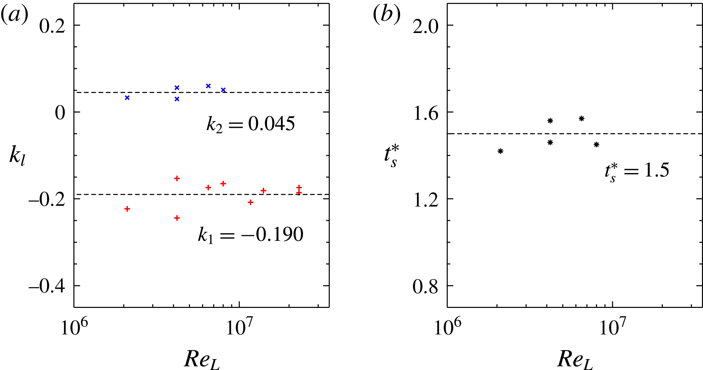
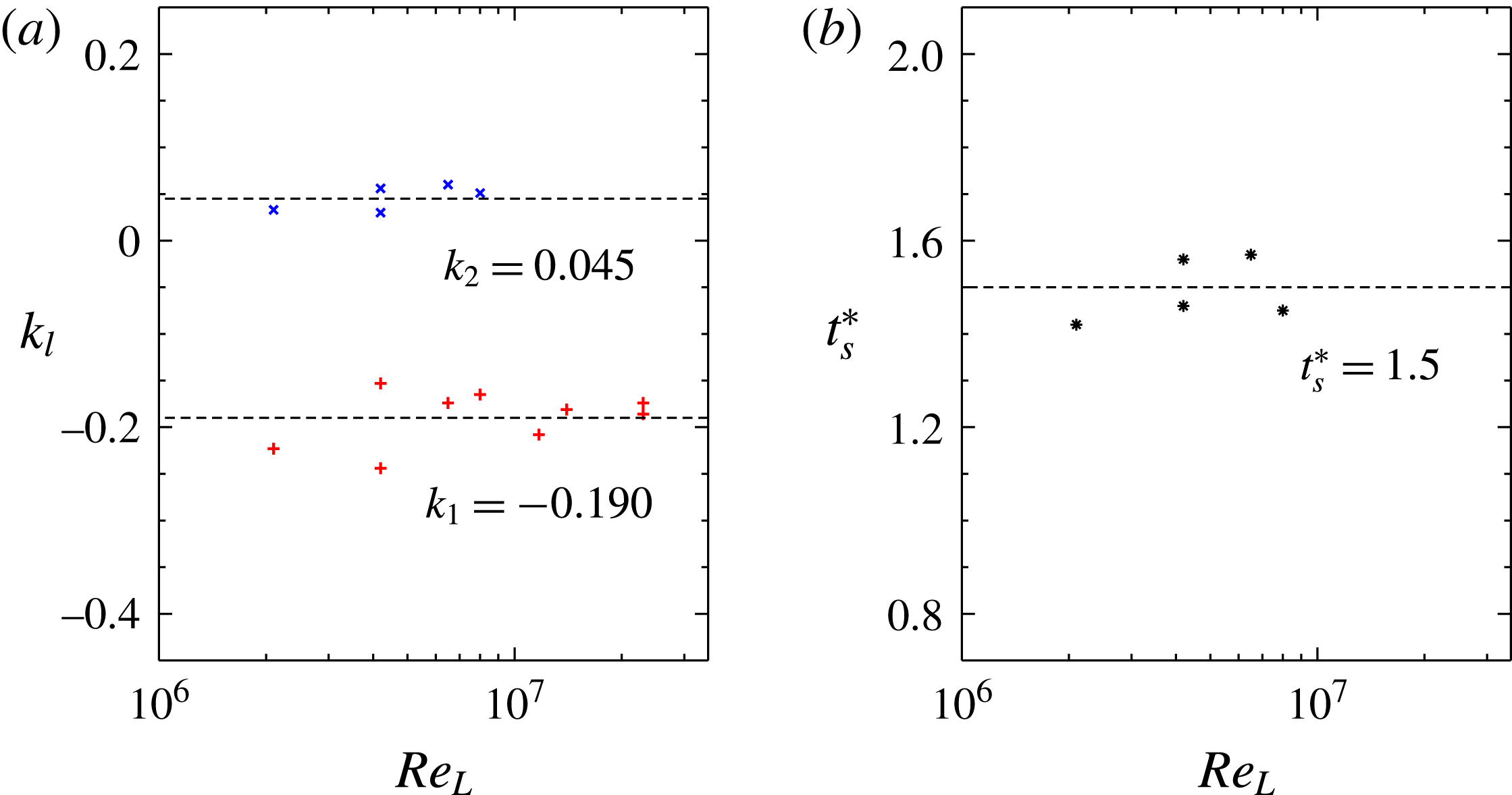
To summarise, the power-law exponent
 $k$
defined by (4.3) can be used as a measure of separation rate to test the effect of the Reynolds number. In figures 7–9, the primary-separation rate
 $k_{1}$
and the secondary-separation rate
 $k_{2}$
are obtained by curve fitting all available data points for each Reynolds number
 $\mathit{Re}_{L}$
. Plots of
 $k_{1}$
and
 $k_{2}$
in figure 10(a) show no strong dependence on the Reynolds number over the range
 $2.1\times 10^{6}\leqslant \mathit{Re}_{L}\leqslant 23\times 10^{6}$
, and so only horizontal lines of best fit
 $k_{1}\simeq -0.190$
and
 $k_{2}\simeq 0.045$
are included as a visual guide. A plot of the start time in figure 10(b) for the same Reynolds-number range shows
 $t_{s}^{\ast }\simeq 1.5$
.
5 Envelope of flow separation
The results in figure 10 established that, for all the different body geometries considered on the axis of
 $\unicode[STIX]{x1D6E9}$
as a function of
 $t^{\ast }$
, the separation rates (
 $k_{1}$
and
 $k_{2}$
) and the start time (
 $t_{s}^{\ast }$
) are not dependent on the Reynolds number over the range
 $2.1\times 10^{6}\leqslant \mathit{Re}_{L}\leqslant 23\times 10^{6}$
. Figure 11 shows a plot of all the data points gathered from figures 7–9; the curves of best fit yield
 $$\begin{eqnarray}\unicode[STIX]{x1D6E9}_{B_{1}^{-}}=151.2(t^{\ast })^{-0.190},\quad \unicode[STIX]{x1D6E9}_{B_{2}^{-}}=137.5(t^{\ast })^{0.045},\end{eqnarray}$$
with an r.m.s. difference of 6.3 % for the primary separation and 2.5 % for the secondary separation, where the curves start at (
 $t_{s}^{\ast }$
,
 $\unicode[STIX]{x1D6E9}_{s}$
)
 $\simeq$
(1.5,
 $140^{\circ }$
). For the fitted curves, altering a least significant digit in each numerical coefficient in (5.1) changes the r.m.s. difference by no more than 1 %, and changes the model prediction of
 $\unicode[STIX]{x1D6E9}_{s}$
by no more than
 $1^{\circ }$
at the start time
 $t_{s}^{\ast }=1.5$
.
Power-law curve fits to all the data points from figures 7–9 for the body-length Reynolds number over the range
 $2.1\times 10^{6}\leqslant \mathit{Re}_{L}\leqslant 23\times 10^{6}$
: (a) primary-separation data, and (b) secondary-separation data. The locus chart constructed from (5.1) shows (I) the initial region, (II) the windward stream, (III) the leeward stream and (IV) the separation envelope.
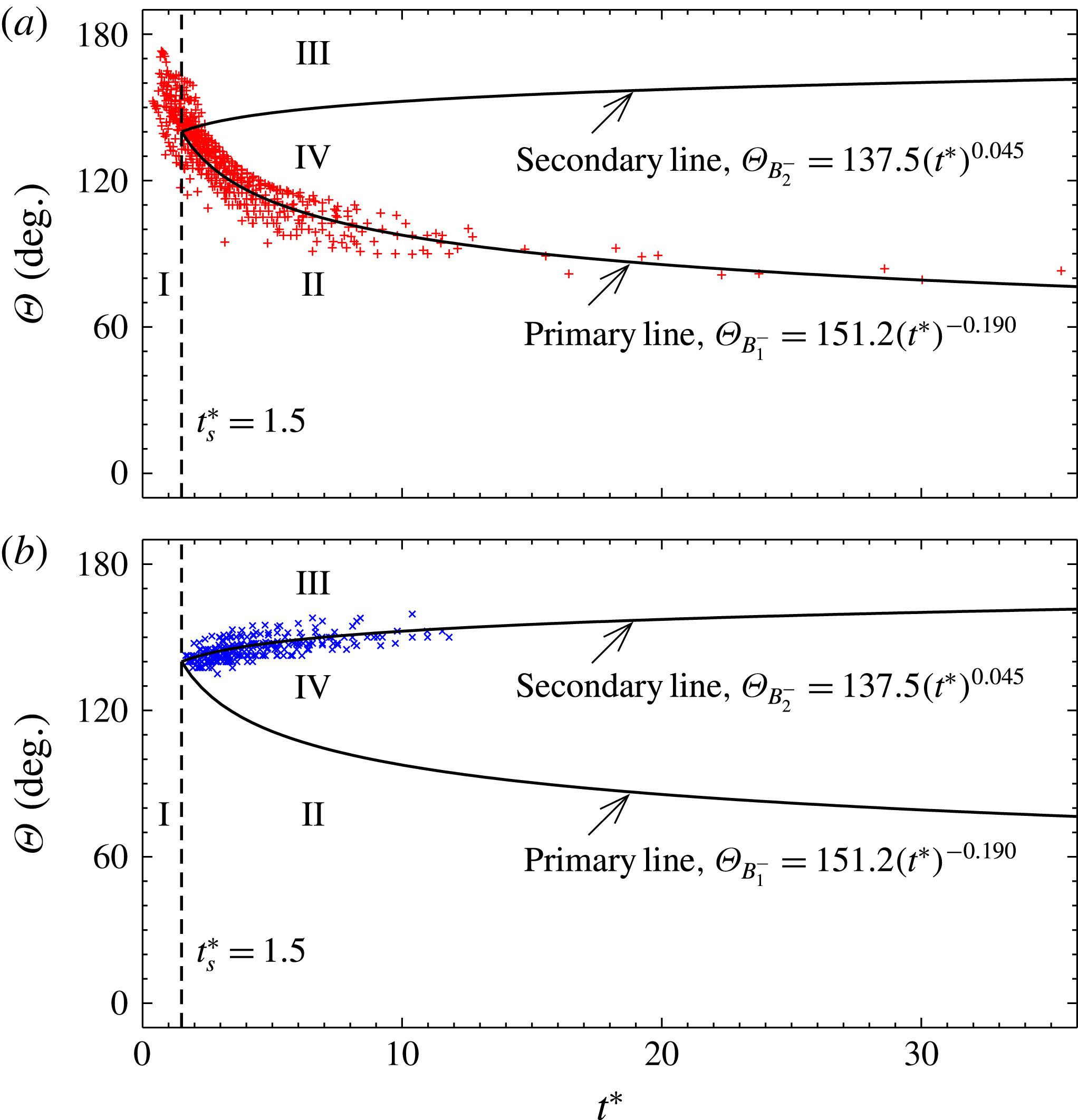
In figure 11, the locus chart constructed from (5.1) summarises four regions of slender-body surface flow. Region ‘I’ in the range
 $t^{\ast }<t_{s}^{\ast }$
represents the initial development of separation over the slender body. Regions ‘II’ and ‘III’ in the range
 $t^{\ast }\geqslant t_{s}^{\ast }$
cover the windward and leeward streams, respectively. Region ‘IV’ defines the envelope of separation between the two streams, where the size of the separation (
 $\unicode[STIX]{x1D6E9}_{B_{2}^{-}}-\unicode[STIX]{x1D6E9}_{B_{1}^{-}}$
) increases at a power-law rate of time
 $t^{\ast }$
.
6 Conclusions
Surface-flow visualisation identifies the primary and secondary leeward-separation lines as key topological features on axisymmetric slender bodies at incidence. For the present collection of data, the incidence angles are between
 $6$
and
 $35^{\circ }$
. The windward side corresponds to the body azimuth angle
 $\unicode[STIX]{x1D6E9}=0^{\circ }$
and the leeward side is at
 $\unicode[STIX]{x1D6E9}=180^{\circ }$
. The development of flow-separation lines is taken as a transient problem which relates the longitudinal distance
 $x$
to time
 $t^{\ast }=x\,\,\text{tan}(\unicode[STIX]{x1D713})/r(x)$
, where
 $r(x)$
is the local body radius and
 $\unicode[STIX]{x1D713}$
is the incidence angle. The separation-line data fall on a power law
 $\unicode[STIX]{x1D6E9}\sim (t^{\ast })^{k}$
. The separation rate
 $k$
does not depend on the body-length Reynolds number over the range
 $2.1\times 10^{6}\leqslant \mathit{Re}_{L}\leqslant 23\times 10^{6}$
, with
 $k_{1}\simeq -0.190$
for the primary line and
 $k_{2}\simeq 0.045$
for the secondary line. The power-law curve fits trace the separation lines to a characteristic start time
 $t_{s}^{\ast }\simeq 1.5$
.
Acknowledgements
Thanks go to P. Jacquemin for operating the DST low-speed wind tunnel and to QinetiQ for manufacturing ancillary components for the slender bodies. This work acknowledges the helpful feedback from fellow DST colleagues and from the anonymous referees.