1. Introduction
After two weeks of hard work and concerted efforts by all the parties involved, the landmark Paris Agreement was reached in December 2015, charting a clear course for global cooperation on fighting climate change to hold the average rise in global temperature well below 2°C above pre-industrial levels and to pursue efforts to limit the temperature increase to 1.5°C (UNFCCC, 2015). For governments around the world, the most urgent task of implementing the details of the agreement is to prepare plans and actions in line with their national priorities to achieve the goals set in their nationally determined contributions. Because energy-intensive sectors are major carbon emitters, it should come as no surprise that climate policies will target these sectors. This will lead to carbon leakage across sectors, given that the products of the regulated sectors are widely used in industrial production as intermediate inputs, such as electricity, and the share of intermediate inputs per unit of outputs increases gradually (Xu and Dietzenbacher, Reference Xu and Dietzenbacher2014). This domestic leakage may in turn offset the carbon reduction of the regulated sectors (Zhang, Reference Zhang2012; Baylis et al., Reference Baylis, Fullerton and Karney2014; World Bank, 2015). This situation highlights that intermediate input linkage may be an important influencing factor of carbon leakage. Böhringer et al. (Reference Böhringer, Müller and Schneider2014) found that domestic industries may suffer rather than benefit from anti-leakage measures under the consideration of an intermediate input structure. The purpose of this study is to clarify the relation between the intermediate input linkage and carbon leakage and to evaluate the leakage effects of China's climate regulations on the electricity generation sector.
The theoretical model of this study builds on a Harberger (Reference Harberger1962) type general equilibrium model aimed at studying the effects of climate policies (e.g., Fullerton and Heutel, Reference Fullerton and Heutel2007; Fullerton and Monti, Reference Fullerton and Monti2013; Lanzi and Wing, Reference Lanzi and Wing2013; Baylis et al., Reference Baylis, Fullerton and Karney2014; Elliott and Fullerton, Reference Elliott and Fullerton2014; Rausch and Schwarz, Reference Rausch and Schwarz2016). However, these studies mainly adopt the assumption of an independent sector or vertical sectoral linkage (e.g., Bushnell and Mansur, Reference Bushnell and Mansur2011; Baylis et al. Reference Baylis, Fullerton and Karney2014; Sen, Reference Sen2015), and a systematic study on the effect of sectoral linkage on carbon leakage is lacking. To capture the impact of sectoral linkage on carbon leakage, we extend the two independent sector model of Baylis et al. (Reference Baylis, Fullerton and Karney2014), by introducing an intermediate input linkage structure. This study disentangles four leakage effectsFootnote 1 and derives closed-form solutions for these effects. All these effects are related to the intermediate input linkage either directly or indirectly.
We find that the intermediate input linkage has important implications for assessing the carbon leakage problem. First, the change in gross output and emissions due to consumption change is influenced by the intermediate input linkage structure directly, which is known as the multiplier effect (ME). Secondly, producers would adjust the intermediate input structure because climate policies result in higher price levels of the energy-intensive products, which is closely related to the production substitution effect (PSE). Thirdly, the intermediate input linkage has an indirect impact on the magnitude of the scale and consumption substitution effects. For instance, close industrial linkage means that the relative price change is small, and the consumption substitution effect (CSE), which reflects the environmental impact of consumption structure adjustment due to relative price change, would be relatively small.
The empirical study of this paper focuses on the effect of climate regulations on the electricity generation sector in China using a computable general equilibrium (CGE) model of China's economy. Electricity not only accounts for the largest share of direct emissions but is also a crucial intermediate input used in most production activities. China's carbon emissions trading pilots pay special attention to the impact of intermediate input linkage on the environmental effect of climate regulations. One key feature of China's carbon trading pilots is the regulation of both direct and indirect emissions from electricity generation (Zhang, Reference Zhang2015a, Reference Zhang2015b). Previous studies (e.g., Bernstein et al., Reference Bernstein, Montgomery and Rutherford1999; Babiker, Reference Babiker2001; Kuik and Gerlagh, Reference Kuik and Gerlagh2003; Mathiesen and Mæstad, Reference Mathiesen and Mæstad2004; Barker et al., Reference Barker, Junankar, Pollitt and Summerton2007; Antimiani et al., Reference Antimiani, Costantini, Martini, Salvatici and Tommasino2013; Meunier et al., Reference Meunier, Ponssard and Quirion2014; Böhringer et al., Reference Böhringer, Rivers and Onezawa2016) have focused mainly on the developed regions’ regulations and on leakages between developed and developing countries. Our study focuses on the carbon leakage of China's climate regulations between a regulated sector and unregulated sectors, and thus will broaden our understanding of carbon leakage and enrich the policy relevance of existing studies.
There is a close relationship between the Harberger-type model and the CGE model, which are adopted for the theoretical and numerical studies of this paper, respectively. Chumacero and Schmidt-Hebbel (Reference Chumacero and Schmidt-Hebbel2004) classify the Harberger-type model as a CGE model. Kortum (Reference Kortum2011) states that the Harberger-type model can be observed as a simpler version of the CGE model. The previous literature links these two models by changing the key parameters of the CGE model (Carbone, Reference Carbone2013) or by inserting parameters taken from a CGE model to the theoretical results (Lanzi and Wing, Reference Lanzi and Wing2013). Adopting structural decomposition analysis (Hoekstra and van den Bergh, Reference Hoekstra and van den Bergh2003), this study proposes another method to link the theoretical and numerical models, and we quantitatively evaluate the magnitude of four leakage effects. The simulation results show that China's climate regulations on the electricity generation sector would generate negative sectoral leakage, which is mainly determined by the PSE and the ME, both of which have a close relation with the sectoral linkage.
This study contributes to the literature in several ways. First, this study clarifies the direct and indirect impacts of intermediate input linkage on carbon leakage of sectoral climate regulations from the perspectives of four different leakage effects. Secondly, the study develops a Harberger-type model with an input-output linkage structure, which can represent two countries linked through the trade of intermediate goods or a closed economy with two interdependent sectors. Thirdly, the study proposes a method to link the theoretical and numerical models by adopting structural decomposition analysis and quantitatively evaluates the magnitude of different leakage effects. The policy implication is that policy makers should consider domestic sectoral linkages in the determination of climate regulations and anti-leakage measures.
The remainder of the paper is organized as follows. Section 2 develops a Harberger-type theoretical model with an input-output linkage structure and derives closed-form expressions of four different leakage effects. Section 3 builds China's CGE model for empirical simulation and introduces structural decomposition analysis to link the theoretical and empirical models. Section 4 discusses the simulation results. The conclusions are presented in section 5.
2. The theoretical model
With the development of production fragmentation, firms in different sectors and regions are more closely connected to each other through intermediate input linkage. Sectoral linkage may have an obvious impact on the environmental effect of climate regulations. In order to present the relation between intermediate input linkage and carbon leakage, this study extends the model presented in Baylis et al. (Reference Baylis, Fullerton and Karney2014), which assumes two independent sectors by introducing a sectoral input-output linkage structure. Our model allows us to quantify the impact of intermediate input linkage on carbon leakage under a small change in the carbon tax. The theoretical model of this study is presented in the following subsection.
2.1 Theoretical model
2.1.1 Production
In a closed economy, two competitive sectors (i, j=X, Y) use intermediate input M
i
, clean input K
i
and carbon emissions E
i
, with decreasing marginal products in a constant return to scale production function. For illustration purposes only, this study assumes that the sector X represents the electricity generation sector and the sector Y represents the other sector. The final output of sector
 $i (O_{i} = f(M_{i} ,K_{i} ,E_{i}))$
satisfies both the final demand of consumers (C
i
) and the intermediate demand of the other sector j (M
j
). The intermediate input share is
 $\xi_{iM} = M_{i} P_{j} /O_{i} P_{i}, (i\ne j)$
. The clean and dirty factor input shares are
 $\xi _{iK} =(1-\xi_{iM}) \theta_{iK}$
and
 $\xi_{iE} =(1-\xi _{iM})\theta_{iE}$
, where θ
iK
and θ
iE
 $(\theta_{iK} +\theta_{iE} =1)$
are the share of clean and dirty inputs to the gross factor input. We assume that the electricity generation sector X has a greater carbon intensity
 $(\xi_{XE} > \xi_{YE})$
. Differentiating each sector's production function, we obtain the following:
 $$\hat{O}_i =\xi_{iM} \hat{M}_i +\xi_{iK} \hat{K}_i +\xi_{iE} \hat{E}_i.$$
The presence of a hat notation above any variable represents each proportional change (e.g.,
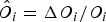 $\hat{O}_{i} =\Delta O_{i} /O_{i}$
).
Firms would adjust the input structure with changes in the relative price, and this corresponds to the PSE. For instance, they would reduce carbon emissions per unit of output by incremental capital investment. The Harberger-type model with three or more inputs usually adopts Allen elasticities of substitution. Karney (Reference Karney2016) proposes a method to switch from Allen to Morishima elasticities and demonstrates a one-to-one numerical equivalence of models using two different elasticities. Therefore, our paper also adopts Allen elasticities of substitution and defines the elasticity of substitution between intermediate and factor inputs as e. We obtain the following:
 $$\left\{\matrix{ \hat{M}_i\,{-}\,\hat{E}_i =\xi_{iM} (e_{MM}^i\,{-}\,e_{EM}^i )\hat{P}_j\,{+}\,\xi_{iK} (e_{MK}^i\,{-}\,e_{EK}^i)\hat{P}_K\,{+}\,\xi_{iE} (e_{ME}^i\,{-}\,e_{EE}^i)\hat{P}_{iE} \cr \cr \hat{K}_i\,{-}\,\hat{E}_i =\xi_{iM} (e_{KM}^i\,{-}\,e_{EM}^i )\hat{P}_j\,{+}\,\xi_{iK} (e_{KK}^i\,{-}\,e_{EK}^i)\hat{P}_K\,{+}\,\xi_{iE} (e_{KE}^i\,{-}\,e_{EE}^i)\hat{P}_{iE}. } \right..$$
The capital is movable across electricity generation sector X and the other sector Y, with the same return (P
K
) and a fixed supply
 $( \overline{K} = K_X + K_Y)$
. Completely differentiating the capital constraint equation
 $\overline{K} = K_{X} + K_{Y}$
, we obtain the following:
 $$\alpha_X \hat{K}_X +\alpha_Y \hat{K}_Y =0,$$
where α
X
and α
Y
are the sectoral share of the capital distribution between two sectors and satisfy
 $\alpha_{X} +\alpha_{Y} =1$
.
2.1.2 Price
Perfect competition and constant returns to scale imply zero profit, so
 $P_{i} O_{i} = P_{j} M_{i} +P_{K} K_{i} + P_{iE} E_{i}$
. Completely differentiating these equations and using companies’ profit-maximizing first-order conditions yields the following:
 $$\hat{P}_i +\hat{O}_i =\xi_{iM} (\hat{P}_j +\hat{M}_i )+\xi_{iK} (\hat{P}_K +\hat{K}_i )+\xi_{iE} (\hat{P}_{iE} +\hat{E}_i).$$
According to equation (1), we find the relationship of the proportional change in price levels,
 $$\hat{P}_i =\xi_{iM} \hat{P}_j +\xi_{iK} \hat{P}_K +\xi_{iE} \hat{P}_{iE}.$$
The price level faced by consumers (Î) is determined by the price level of two sectors
 $(\hat{I}={C_{X} \Delta P_{X} +C_{Y} \Delta P_{Y} \over C_{X} P_{X} +C_{Y} P_{Y}}={C_{X} P_{X} \over C_{X} P_{X} +C_{Y} P_{Y} }\Delta P_{X} /P_{X} +{C_{Y} P_{Y} \over C_{X} P_{X} +C_{Y} P_{Y} }\Delta P_{Y} /P_{Y} )$
. Supposing ϑ
i
is the share of income spent on sector
 $i (\vartheta_{i} =P_{i} C_{i} /(P_{i} C_{i} +P_{j} C_{j} ), (i\ne j))$
, we obtain the following:
 $$\hat{I}=\vartheta_X \hat{P}_X +\vartheta_Y \hat{P}_Y.$$
According to the production approach of nominal gross domestic product (GDP) (N), the mathematical expression is
 $N=(1-\xi_{YM} )O_{X} P_{X} +(1-\xi_{YM} )O_{Y} P_{Y}$
. Taking the logs and totally differentiating, we obtain the following:
 $$\hat{N}={\vartheta_X +\xi_{YM} \vartheta_Y \over 1-\xi_{XM} \xi_{YM} }(1-\xi_{XM} )(\hat{O}_X +\hat{P}_X )+{\xi_{XM} \vartheta_X +\vartheta_Y \over 1-\xi_{XM} \xi_{YM} }(1-\xi_{YM} )(\hat{O}_Y +\hat{P}_Y).$$
The real GDP (G) satisfies G=N/I. Taking the logs and totally differentiating, we obtain
 $\hat{G}=\hat{N}-\hat{I}$
. Climate regulations would influence the real GDP and the final emissions. The scale effect (SE) of carbon leakage is obtained from the change in real GDP.
2.1.3 Consumption
We assume that all tax revenue (
 $R=P_{XE} E_{X} +P_{YE} E_{Y})$
is returned to individuals via a lump-sum rebate. Under the budget constraint
 $(r \overline{K} + R\ge P_{X} C_{X} +P_{Y} C_{Y} )$
, identical individuals maximize homothetic utility (
 $U(C_{X}, C_{Y}; E_{total}))$
by choosing products from the two sectors. This paper assumes that the welfare gain from carbon reduction
 $(\Delta E_{total} =\Delta E_{X} +\Delta E_{Y})$
is separable in utility (Baylis et al., Reference Baylis, Fullerton and Karney2013) and focuses on the welfare effects from consumption. Under the assumption that pollution is separable in utility, we define σ
u
as the elasticity of substitution in utility between different products:
 $$\hat{C}_X -\hat{C}_Y =\sigma_u (\hat{P}_Y -\hat{P}_X).$$
Consumers tend to consume more of the products with a relatively lower price level and less of the more expensive products. We obtain the CSE of carbon leakage. According to the product market clearance assumptionFootnote
2
and the intermediate input share, we obtain
 $O_{i} P_{i} =C_{i} P_{i} +\xi_{jM} O_{j} P_{j}, (i\ne j)$
. Completely differentiating the above two equations yields the following:
 $$\hat{O}_i = \hat{C}_i +{(\sigma_u -1)\xi_{jM} \vartheta_j \over \vartheta_i +\xi_{jM} \vartheta_j}(\hat{P}_i -\hat{P}_j), (i\ne j).$$
Equation (8) shows that the output change is not only determined by the final consumption change but is also influenced by the intermediate input structure through the ME. In addition, equation (8) shows that the ME has a close relation with the consumption substitution elasticity. σ
u
=1 means that the share of income spent on electricity and other products is fixed
 $(\hat{C}_{X} +\hat{P}_{X} =\hat{C}_{Y} +\hat{P}_{Y})$
. Then, the final output has a linear relation with the final consumption, and the rates of percentage change in these two variables are the same.
2.1.4 Climate policy
We assume that climate regulation applies only to the electricity generation sector X, which has a greater carbon intensity.
 $$\hat{P}_{XE} =\tau$$
 $$\hat{P}_{YE} = 0.$$
In addition, this paper assumes that the capital price level is chosen as the numeraire P̂K =0. There are 18 variables and 18 equations for the theoretical analytical framework, and the model is solvable mathematically. The parameters, variables and equations of the theoretical model are summarized in appendix A.
2.2 Decomposition analysis of theoretical results
The proportional change in carbon emissions of the unregulated sector can be explained by four different effects: the scale effect (SE), the consumption substitution effect (CSE), the multiplier effect (ME), and the production substitution effect (PSE).
 $$\hat{E}_Y =SE+CSE+ME+PSE$$
The derivation of equation (11) is presented in appendix B. The environmental effects of climate policies through the expansion or contraction of the overall economic scale, which is represented by the real GDP (G), is named the scale effect (SE). The mathematical expression of the percentage change of G is represented by parameters and the exogenous policy shock. The results show that the SE is related to the intermediate input linkage through two different mechanisms. First, the SE is influenced by the intermediate input linkage structure, which is represented by the intermediate input coefficient (ξ
XM
and ξ
YM
). Under the extreme case that two sectors are independent (
 $\xi_{XM} =\xi_{YM} =0)$
, we obtain
 $\hat{G}=-\alpha_{X} (e_{KE}^{X} -e_{EE}^{X} )\theta_{XE} \theta _{XE} \tau -(\vartheta_{X} \alpha_{Y} -\vartheta_{Y} \alpha_{X} )\sigma_{u} \theta_{XE} \tau $
. We can prove that climate regulations under the carbon-intensive sectors will reduce the gross economic scaleFootnote
3
if we ignore the intermediate input linkage. Secondly, the SE has a close relation with the intermediate substitution elasticity of both the electricity generation sector X and the other sector Y (
 $e_{ME}^{X} $
,
 $e_{KM}^{Y} $
and
 $e_{EM}^{Y} )$
. This reflects the impact of intermediate input linkage change on the environmental effect of climate regulations indirectly through the SE.
The climate policies shock the final price level faced by consumers, and the changes in final prices are
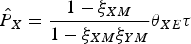 $\hat{P}_{X} ={1-\xi_{XM} \over 1-\xi_{XM} \xi_{YM} }\theta_{XE} \tau $
and
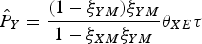 $\hat{P}_{Y} ={(1-\xi_{YM} )\xi_{YM} \over 1-\xi_{XM} \xi_{YM} }\theta_{XE} \tau $
. When ξ
YM
<1, we obtain
 $\hat{P}_{X} >\hat{P}_{Y} $
. This means that the consumer will face a relatively higher electricity price level (sector X). Then, consumers will adjust their consumption structure and improve the share of consumption on products of the other sector Y. The environmental impact of a consumption structure adjustment due to a relative final price change is named the consumption substitution effect (CSE). When ξ
XM
=1 or ξ
YM
=1, all products of sector Y or X are used to satisfy the intermediate demand, and the products of the two sectors are not substitutes. Therefore, the consumption substitution will be zero.
 ${dCSE \over d\xi_{XM} }<0$
and
 ${dCSE \over d\xi _{YM} }<0$
, which means that the closer the sectoral linkage is, the smaller the change in relative final price levels will be and the scale of the CSE will be much smaller.
The ME influences the environmental effects of climate policies by impacting the volume change of final products due to changes in final demand. The sign of ME is determined by the consumption substitution elasticity. The final output and final consumption of the unregulated sector satisfy
 $(1-\xi_{XM} \xi_{YM} )O_{Y} P_{Y} =\xi_{XM} C_{X} P_{X} + C_{Y} P_{Y} $
.Footnote
4
When σ
u
=1, the expenditure structure remains consistent. We can obtain that the final output and consumption will share the same percentage change (
 $\hat{O}_{Y} =\hat{C}_{Y} )$
, and the ME has no influence on the rate of change of these two variables. σ
u
>1 means that the expenditure share has a negative relation with the relative price level, and consumers would decrease the share of gross income spent on unregulated products; therefore, the sign of ME is negative. σ
u
<1 means that consumers will increase the expenditure share of unregulated products, and the sign of ME is positive. In addition, the ME is closely related to the intermediate input coefficient. When ξ
XM
=0, climate regulations on the upstream firms will face a zero ME of the regional carbon leakage because the products of the downstream industry are used to satisfy the final consumption.
Climate policies would shock the production structure, and the environmental effect of the production structure change caused by climate regulations is called the production substitution effect (PSE). The PSE is made up of two parts. The first part is related to the intermediate input structure change, and the second part is related to the factor input structure change. Climate regulations would increase the electricity price level, and the unregulated sector would reduce the intermediate demand for electricity and increase the factor demand. In addition, producers would adjust the factor input structure with the relative price change. The sign of the PSE is determined by the substitution elasticity. We can see that the sign of the PSE is ambiguous. The mathematical expression of carbon leakage appears to be complex, but we can obtain several simplified forms for special cases. For instance, when substituting the sectoral interdependence (ξ XM =0 and ξ YM =0), the theoretical results are consistent with the model of Baylis et al. (Reference Baylis, Fullerton and Karney2014).Footnote 5
3. The numerical model
The theoretical model shows the potential impact of the intermediate input linkage on the problem of carbon leakage and demonstrates the importance of considering sectoral linkage when discussing carbon leakage. Given that electricity is widely used in industrial production as intermediate inputs and the electricity generation sector is a key target of climate regulations, we take the electricity generation sector as a case to quantitatively evaluate the magnitude of four different leakage effects identified in the theoretical model. To that end, this study builds a CGE model of China's economy and introduces structural decomposition analysis to link both the theoretical and empirical models.
3.1 Computable general equilibrium model
The CGE model describes the behaviors of different economic agents (the government, households and enterprises) using a system of equations. To minimize costs, enterprises use intermediate inputs and factor inputs to produce products, subject to certain technological constraints. Households choose domestic and imported products to maximize their utility under budget constraints. As a tax collector, the government determines its expenditures, transfers and savings, according to tax revenues. The static CGE model constructed by this paper is made up of four blocks: production, consumption and trade, emissions and policy, equilibrium and closure.Footnote 6 The database is the social accounting matrix (SAM) of China in 2007, which is obtained from the Development Research Center of the State Council. To reflect the substitution among different types of electricity, this paper decomposes the electricity generation sector into the thermal power sector, the hydropower sector and the nuclear power sector. Refer to appendix C for the 44 sectors discussed in this study. The sectoral carbon emissions are calculated based on the fossil fuel demand (NBS, 2008) and carbon emission factors (IPCC, 2006).
3.1.1 Production
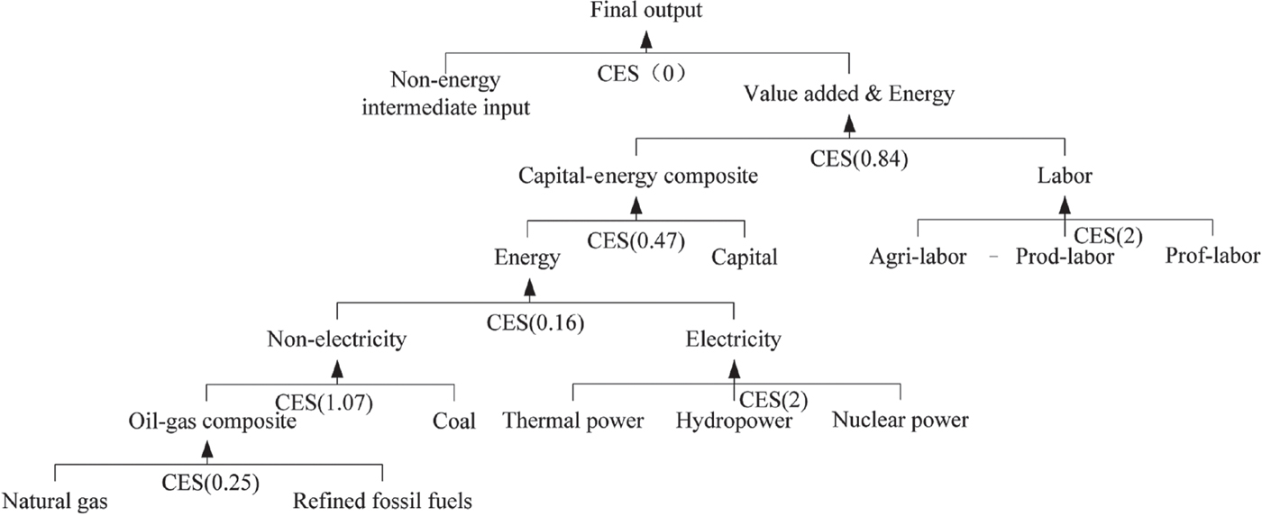
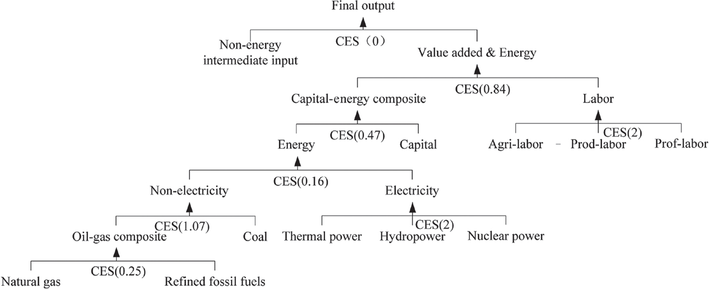
The production technology is represented by a five-stage nested constant elasticity of substitution (CES) production function. The nesting structure of production is shown in figure 1. Being taken out of the intermediate input nest, the energy is incorporated into the value-added nest. The final output is the compositions of value-added energy composite and intermediate inputs through a Leontief function. The value-added energy composite is the composition of the capital-energy composite and labor. Labor is divided into agricultural labor, production labor and professional labor. Energy is divided into electricity and non-electricity. The electricity is provided by thermal, hydroelectric and nuclear power plants. Non-electricity is the composition of coal and non-coal, which is made up of natural gas and refined fossil fuels. The energy substitution elasticities used in this paper are derived from the existing literature (Beckman et al., Reference Beckman, Hertel and Tyner2011; Stern, Reference Stern2012). The capital/energy/labor substitution elasticities are obtained from Lv et al. (Reference Lv, Guo and Xi2009).
Production structure of the computable general equilibrium model
Consumption structure of the computable general equilibrium model

3.1.2 Consumption and trade
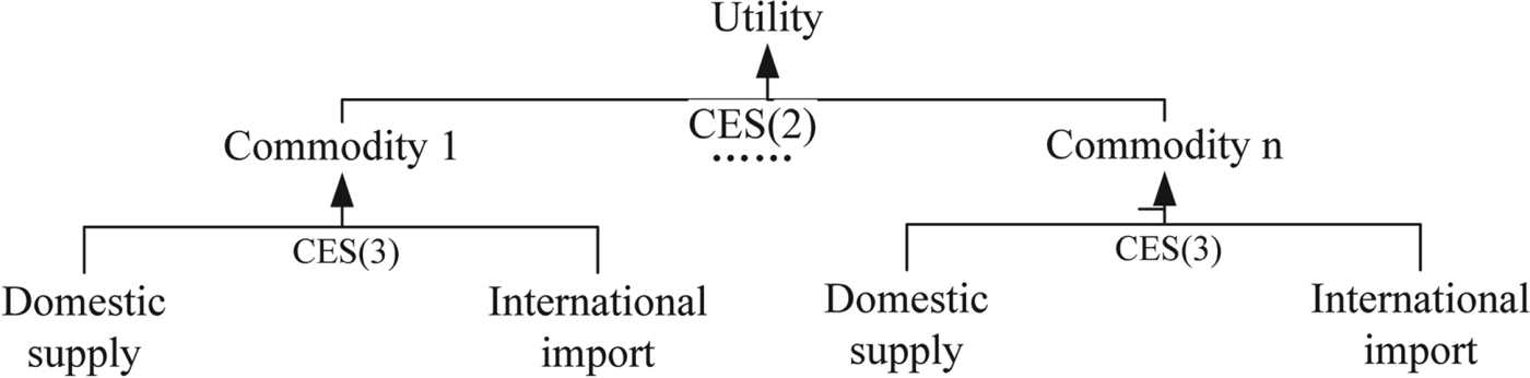
Households earn income from the factor return and government transfer. All the income is spent on commodities, direct taxes and household savings. To maximize the utility, households’ behaviors are described by the CES function. The consumption demand for certain products is positively related to the real income level and is negatively related to the price level. Under climate regulations, consumers will adjust their consumption structure with the change of income and price levels. The enterprise earns revenue by sold products. The revenue is spent on intermediate goods, transferred to a household through factor return, and paid in taxes to the government. The total domestic demand for manufactured goods is determined by the intermediate input demand of enterprises, the final consumption demand of households and the government, and products exported to foreign countries. This demand pool is satisfied by a combination of goods produced by different companies in the domestic market and other regions. We assume that the products of different regions compete as imperfect substitutes (the Armington assumption). The elasticity parameters are obtained from the previous literature (Tarr, Reference Tarr2012).
3.1.3 Emissions and policy
The sectoral emissions are calculated by multiplying the demand for different fossils by the carbon emissions factors. Under the complete information and perfect competition assumption, the CGE model assumes that the carbon price is equal to the trading price of carbon permits. Qi and Cheng (Reference Qi and Cheng2015) note that the difference in the carbon price of the seven carbon trading pilots decreases gradually, ranging from Yuan 24 to 55 per ton. China's seven carbon emissions trading pilots all cover both direct and indirect emissions from electricity. This study simulates the effect of pricing carbon at Yuan 30 per ton in the electricity sector. All tax revenues will be returned to the households through transfer payments. For simplicity, the study assumes that the carbon abatement cost of the electricity generation sector can be passed through to the downstream industries directly.Footnote 7
3.1.4 Equilibrium and closure
The CGE model incorporates the commodity market, factor market and exchange market of domestic and foreign products. The equilibrium module presents the clearance of each market. For instance, commodity market clearance implies that the value of gross output equals the sum of intermediate input and final demands. The closure module describes the balance of saving and investment, government budget and international payments. This paper adopts the neoclassical closure principle. First, total investment in the economy is adjusted to the gross savings (household savings, corporate savings, government savings, public sector surplus earnings and foreign savings) to balance the savings-investment closure. Secondly, the tax rate, transfer payments and government consumption are fixed, whereas government savings are endogenous to balance the government budget closure. Thirdly, the exchange rate is endogenously determined to balance the international payments.
3.2 Structural decomposition analysis
Using the numerical model presented above, we can simulate the economic and environmental effects of climate regulations on the electricity generation sector. However, the CGE model reports only the single net aggregated simulation result without showing the fact that different effects may offset each other (Baylis et al., Reference Baylis, Fullerton and Karney2014). This study introduces a structural decomposition analysis to numerically evaluate the four different leakage effects presented in the theoretical model. We suppose that G represents the real GDP, S represents the sectoral share of final demand, B represents the Leontif matrix (1−A)−1, and F represents the sectoral carbon matrix, which is related to the energy consumption structure and carbon emission coefficient of the fossil energy. The sectoral direct emissions satisfy
 $$E = FBSG.$$
According to the structural decomposition analysis, the change in sector emissions is presented below:
 $$\eqalign{ E^{\prime} -E^0 &= F^{\prime} B^{\prime} S^{\prime} G^{\prime} -F^0 B^0 S^0 G^0 \cr & =\underbrace {F^0S^0(G^{\prime} -G^0)}_{{\rm SE}}\underbrace {+F^0(S^{\prime} -S^0)^{\prime} G^{\prime} }_{{\rm CSE}}\underbrace {+F^0(B^0-I)(S^{\prime} G^{\prime} -S^0G^0)}_{{\rm ME}} \cr &\quad \underbrace {+(F^{\prime} B^{\prime} -F^0B^0)S^{\prime} G^{\prime} }_{{\rm PSE}} }.$$
The first part reflects the environmental effect of climate regulations due to the change in the gross economic scale, which reflects the SE. The second part reflects the change of carbon emissions due to the change in the consumption structure, which is related to the CSE. The intermediate input linkage (B 0−I) has an amplification effect on the scale and CSEs of carbon leakage, which represents the ME. Consistent with the theoretical model, the fourth part reflects the PSE, which is related to both the change in the intermediate input structure and energy consumption structure.
4. Numerical results
This section presents numerical simulations of the economic and environmental effects of carbon regulation. Climate regulations on the electricity generation sector have a negative impact on the economy scale, represented by real GDP. The results show that the rate of change of real GDP is −0.35 per cent, which means that the carbon pricing would put downward pressure on China's economic growth in the short term. In addition, climate regulations would drive up the electricity price level, which would increase by 3.40 per cent. The higher electricity price level would further raise the production cost of other sectors. For instance, the price level of chemical products would increase by 1.0 per cent. The consumer price index (CPI) would increase by 0.49 per cent.
Climate regulations have a negative impact on employment. The simulation results show that the employment for production labor decreases by 0.13 per cent, followed by agricultural (−0.10 per cent) and professional labor (−0.09 per cent). Climate regulations on electricity have a more significant impact on the production labor. From an environmental perspective, the gross emissions and carbon intensity decrease by 3.69 and 3.35 per cent, respectively. The carbon pricing will help to achieve China's target of a 40–45 per cent carbon intensity reduction by 2020, compared to 2005 levels. In addition, climate regulations on the electricity generation sector would promote the development of renewable energy, which is represented by hydropower and nuclear power in this present study. We found that the output of renewable energy would increase by 1.80 per cent.
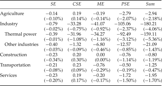
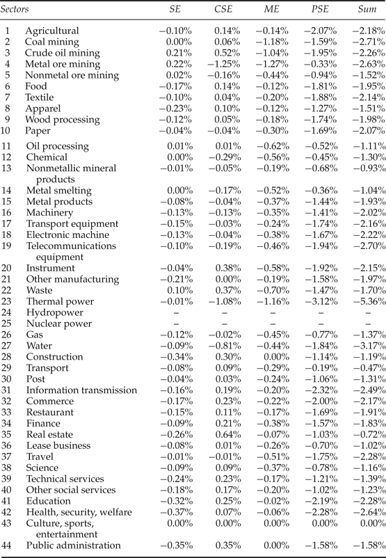
We further present the environmental effects of climate regulation and decompose the change in sectoral emissions into different terms. The aggregated results are presented in table 1 and the decomposition of changes in sectoral emissions is presented in appendix B.
Decomposition analysis of environmental effects of climate regulations (million tons of CO2 emissions)

Notes: The number in parentheses represents the change rate of sectoral emissions (%). SE: scale effect; CSE: consumption substitution effect; ME: multiplier effect; PSE: production substitution effect.
As shown in table 1, we decompose the change in sectoral emissions into four components: the SE, the CSE, the ME and the PSE. The first four columns present the volume and percentage changes in sectoral emissions due to four different effects, and the last column shows the overall change. The results show that the carbon emissions of the thermal power sector decrease by 5.36 per cent, and the carbon emissions of other unregulated sectors decrease by 1.36 per cent. Notably, the other unregulated industries face the greatest scale of carbon reduction (−21.09 million tons of CO2 emissions) because industrial firms are more sensitive to the electricity price level. Defined as the share of the change in unregulated-sector emissions to the reduction in regulated-sector emissions, the sectoral carbon leakage rate is −17.62 per cent.
Wu et al. (Reference Wu, Fan and Xia2016) analyzed the carbon leakage problem faced by carbon emissions trading in China and found that more than 90 per cent of non-trading sectors experience carbon reduction under all scenarios, which is mainly explained by the perspective of input-output linkages. It should be noted that the sectoral carbon leakage rate of the present study is lower than that of Wu et al.’s (2016) study because these two studies choose different sectors as regulated ones. Wu et al. (Reference Wu, Fan and Xia2016) assume that the carbon trading system covers eight energy and energy-intensive industries, whereas this paper focuses only on carbon pricing on the electricity generation sector. The energy-intensive sectors tend to face a greater scale of carbon reduction; therefore, the carbon leakage rate of this paper is lower than that of Wu et al.’s (2016) study.
The numerical simulations show that imposing a carbon price of Yuan 30 per ton on China's electricity generation sector would decrease the GDP by 0.35 per cent. This explains the negative sign of the SE on the emissions of unregulated sectors. For example, the final demand for products of the construction sector would decrease as the GDP decreases. The SE contributes to a decrease in carbon emissions of the construction sector (0.34 per cent). Carbon pricing regulation would increase the electricity price level and the price of other sectors that use electricity as an intermediate input. The industrial sector is more sensitive to electricity prices and would have a relatively higher price level than the other unregulated sectors. Consumers adjust the consumption structure, and the CSE leads to increases in carbon emissions of the products from the agricultural, construction, transportation and service sectors. This is consistent with the theoretical model that the CSE contributes to positive carbon leakage. The change in final demand will influence the sectoral outputs through sectoral linkage, which has an amplification effect on environmental effects. Table 1 shows that the ME contributes to negative carbon leakage. For example, the negative carbon leakage for the transportation sector is mainly induced by the ME. In addition, climate regulations shock the intermediate input structure. The climate regulation encourages firms to use cleaner intermediate and factor inputs, so the PSE corresponds to negative carbon leakage for all sectors. Both the ME and the PSE are closely related to sectoral linkage.
5. Conclusions
Climate regulations tend to cover a limited number of energy-intensive sectors, leading to carbon leakage across sectors. Considering that the regulated products, such as electricity, are widely used in industrial production as intermediate inputs, we attempt to disentangle the influencing mechanism of intermediate input linkage on the problem of carbon leakage.
This present study develops a Harberger-type model considering the sectoral intermediate input linkage structure and provides closed-form solutions for four leakage effects. We find that intermediate input linkage has important implications for assessing carbon leakage. The sectoral linkage directly impacts carbon leakage through the ME, and producers could adjust the intermediate input structure due to climate policies, which is related to the PSE. In addition, the sectoral linkage has an impact on the magnitude of the SE and the CSEs. The present study builds a CGE model of China's economy, proposes a method to link the theoretical and numerical models by adopting structural decomposition analysis and examines the effects of China's climate regulations on the electricity generation sector. The numerical results show that climate regulations on the electricity generation sector would result in significant leakage, which is mainly determined by the PSE, followed by the ME. Both effects are closely related to sectoral linkage. This highlights the importance of considering intermediate input linkage when discussing the problem of carbon leakage.
There are several potential extensions. First, the theoretical model constructed by this study can also represent two countries linked through the intermediate product trade, which could be adopted to analyze the regional carbon leakage of unilateral climate policies. Secondly, this study discusses only four different carbon leakage effects. Future studies could discuss other leakage channels omitted by this study. Thirdly, the empirical study adopts parameters from the literature rather than estimating them econometrically. The theoretical model shows that carbon leakage is sensitive to substitution elasticities; therefore, future studies should address this issue. Finally, this study discusses the environmental effect of China's climate regulations on the electricity generation sector, and the analytical framework of this study can be adopted to discuss the climate policies of other regions.
Appendix A: Parameters, variables and equations of the theoretical model
Parameters, variables and equations of the theoretical model

Appendix B: The derivation of equation (11)
The SE is represented by real GDP (G). The mathematical expression of the percentage change of G is shown below.
 $$\eqalign{SE &= \hat{G} \cr &=\left\{{(\vartheta_X + \xi_{XM} \vartheta_Y )(1-\xi_{XM} ) \alpha_Y -(\xi_{XM} \vartheta_X +\vartheta_Y )(1-\xi_{YM}) \alpha_X \over 1-\xi_{XM} \xi_{YM}} \right. \cr & \quad \times \left(\sigma_u +{(1-\sigma_u )\xi_{YM} \vartheta_Y \over \vartheta_X +\xi_{YM} \vartheta_Y} + {(1-\sigma_u )\xi_{XM} \vartheta_X \over \xi_{XM} \vartheta_X +\vartheta_Y} \right) {(1-\xi_{XM} )(\xi_{YM} -1)\over 1-\xi_{XM} \xi_{YM} }\theta_{XE} \cr & \quad +{(\vartheta_X +\xi_{YM} \vartheta_Y )(1-\xi_{XM} ) + (\xi _{XM} \vartheta_X +\vartheta_Y )(1 - \xi_{YM}) \over 1-\xi_{XM} \xi_{YM}} \cr & \quad \times (1-\xi_{XM} ) \left[ \xi_{XM}\alpha_X(e_{ME}^X -e_{KE}^X ) - (1-\xi_{XM}) \alpha_X (e_{KE}^X -e_{EE}^X)\theta_{XE} \right. \cr & \quad +\left. {\xi_{YM}^2 \over 1-\xi_{XM} \xi_{YM} }\alpha_Y (e_{MM}^Y -e_{KM}^Y )+{\xi_{YM} (1-\xi_{YM} ) \over 1-\xi_{XM} \xi_{YM} }\alpha_Y (e_{KM}^Y -e_{EM}^Y )\right] \theta_{XE} \cr & \quad + \left. {(1-\xi_{XM} )\xi_{YM} \vartheta_Y +\xi_{XM} (\xi_{YM} -1)\vartheta_X \over 1-\xi_{XM} \xi_{YM}} {(1-\xi_{XM} )(1-\xi_{YM} ) \over 1-\xi_{XM} \xi_{YM}} {\theta_{XE}} \right\} \tau}$$
The closed-form solution for the percentage change of the real GDP is represented by parameters and the exogenous policy shock. The final output and final consumption satisfy
 $O_{i} P_{i} =C_{i} P_{i} +\xi_{jM} O_{j} P_{j}$
, and we obtain
 $(\hat{O}_{i} +\hat{P}_{i}) = {\vartheta_{i} (\hat{C}_{i} +\hat{P}_{i}) \over \vartheta_{i} +\xi_{jM} \vartheta_{j} } + {\xi_{jM} \vartheta_{j} (\hat{C}_{j} +\hat{P}_{j} ) \over \vartheta_{i} +\xi_{jM} \vartheta_{j}}$
.
Inserting them into equation (6), we obtain
 $\hat{N}=\vartheta_{X} (\hat{C}_{X} +\hat{P}_{X} )+\vartheta_{Y} (\hat{C}_{Y} +\hat{P}_{Y})$
. This can be observed as the mathematical expression of real GDP under the expenditure approach. According to the relation between real and nominal GDP
 $\hat{G}=\hat{N}-\hat{I}$
, we obtain
 $$\hat{G}=\vartheta_X \hat{C}_X +\vartheta_Y \hat{C}_Y .$$
According to the relation that GDP under the production and expenditure approaches share the same results, we obtain
 $\vartheta_{X} \hat{C}_{X} +\vartheta_{Y} \hat{C}_{Y} =SE$
. The CSE is obtained according to the consumption substitution relationship between two products, which is represented by equation (7). The mathematical expression of consumption demand for products of sector Y is shown below:
 $$\hat{C}_Y =SE\underbrace {+{\sigma_u \vartheta_X (1-\xi_{XM} )(1-\xi_{YM} )\theta_{XE} \over 1-\xi_{XM} \xi_{YM} }\tau }_{CSE}.$$
The final output change due to consumption change is influenced by the intermediate input linkage through the multiplier effect (ME), which is obtained based on the relationship between final consumption and total outputs, represented by equation (8). The mathematical expression is shown below:
 $$\hat{O}_Y =SE+CSE\underbrace {+{(1-\sigma_u )\vartheta_X \xi_{XM} (1-\xi_{XM} )(1-\xi_{YM} )\theta_{XE} \over 1-\xi_{XM} \xi_{YM} }\tau }_{ME}.$$
The PSE is obtained according to the production substitution relationship between factor and intermediate inputs, represented by equation (2).
 $$\eqalign{\hat{E}_Y &= SE + CSE + ME \cr & \quad + \underbrace{\left[{\xi_{YM} \xi_{YM} (1-\xi_{XM} )\theta_{XE} (e_{EM}^Y -e_{MM}^Y ) \over 1-\xi_{XM} \xi_{YM} }+ {\xi_{YK} \xi_{YM} (1-\xi_{XM} )\theta_{XE} (e_{EM}^Y -e_{KM}^Y ) \over 1-\xi_{XM} \xi_{YM}}\right]\tau}_{PSE}}$$
Appendix C: Decomposition analysis of sectoral emissions change
Decomposition analysis of sectoral emissions change