1 Introduction
Our interest is the complex, three-dimensional wake immediately aft of the dry transom stern of a surface ship. This region contains violent breaking of the free surface, highly mixed air–water turbulent flow, large-scale air entrainment and air cavity breakup. We present this work in two parts. In Part 1 (Hendrickson et al. Reference Hendrickson, Weymouth, Yu and Yue2019), we focus on the wake surface, the structure of the underlying wake flow, Lagrangian characteristics of the large-scale air entrainment and surface entrainment rate and the scaling of these with Froude number and stern geometry. The objective of Part 1 is to provide a physical understanding of the detailed flow features in the mixed region and the characteristics of the large-scale air entrainment. Part 2 focuses on understanding and modelling of the highly mixed, air–water turbulent near-surface region of the wake by combining the surface fluctuations, spray and entrainment into a single mixed-phase region through an Eulerian framework. The objective of Part 2 is to provide a statistical understanding of the mixed-phase region within the context of incompressible highly variable density turbulence (IHVDT) and address the necessary turbulent closure modelling.
The turbulent air entraining ship-wake problem presents a special class of variable density turbulent flows with experimental and computational challenges. The problem involves high void fractions (20 %–30 %) (Terrill & Fu Reference Terrill and Fu2008) and the ship-scale problem spans 7–8 orders of magnitudes in flow length scales. Until recently, relatively little was understood about the turbulent nature of this flow. Many experiments and simulations provide insight into the mean flow and turbulent nature of real ship wakes in the absence of entrainment (Sotiropoulos & Patel Reference Sotiropoulos and Patel1995; Gui, Longo & Stern Reference Gui, Longo and Stern2001; Kim, Van & Kim Reference Kim, Van and Kim2001; Olivieri et al. Reference Olivieri, Pistani, Avanzini, Stern and Penna2001; Shen, Zhang & Yue Reference Shen, Zhang and Yue2002; Larsson, Stern & Betram Reference Larsson, Stern and Betram2003). Part 1 provides a detailed review of the known air entrainment characteristics and surface features of transom wake flows. To date, a detailed understanding of the turbulent nature of the mixed-phase region of the flow remains elusive.
There is significant information available on miscible incompressible variable density turbulent flows such as the buoyancy-driven Rayleigh–Taylor instability (Sharp Reference Sharp1984; He et al. Reference He, Zhang, Chen and Doolen1999; Livescu & Ristorcelli Reference Livescu and Ristorcelli2007, Reference Livescu and Ristorcelli2008) and mixing by jets (List Reference List1982; Dimotakis Reference Dimotakis2005). In the category of immiscible fluids, there is a substantial literature on such topics as bubble columns (Mudde Reference Mudde2005) and swarms (Lance & Bataille Reference Lance and Bataille1991; Bunner & Tryggvason Reference Bunner and Tryggvason2002a ,Reference Bunner and Tryggvason b ). In these turbulent dispersed multiphase flows, the driving mechanism derives from the gas flow and the bubble-induced velocity/turbulence is non-negligible. More convective bubbly flows include hydraulic jumps (Chachereau & Chanson Reference Chachereau and Chanson2011; Mortazavi et al. Reference Mortazavi, Le Chenadec, Moin and Mani2016), cavitating hydrofoils and ventilated bodies (Karn et al. Reference Karn, Shao, Arndt and Hong2016; Kang et al. Reference Kang, Zhang, Gu and Mao2017; Young et al. Reference Young, Harwood, Miguel Montero, Ward and Ceccio2017). In Part 1, we show that the near-wake flow of the stern bears little similarity to that of hydraulic jumps. From the perspective of shear wakes, while there is a significant literature on cavitating bodies, there is sufficient difference in the wakes between naturally ventilated and cavitating bodies to warrant separate investigations (Young et al. Reference Young, Harwood, Miguel Montero, Ward and Ceccio2017). Finally, and unfortunately, the literature on ventilated bodies focuses mainly on the hydrodynamic forcing rather than the wake IHVDT. When we consider the literature as a whole, there is little knowledge or guidance for the problem considered here.
For turbulent dispersed multiphase flows, the particle Stokes number
 $S_{t}=(\unicode[STIX]{x1D70F}_{p}/\unicode[STIX]{x1D70F}_{k})$
, where
 $\unicode[STIX]{x1D70F}_{p}$
is the particle time scale and
 $\unicode[STIX]{x1D70F}_{k}$
the Kolmogorov time scale, is key to determining if the surrounding fluid dictates the particle’s motion (rather than its own momentum and energy). For
 $S_{t}\lesssim 0.2$
, this assumption is fairly accurate (Balachandar & Eaton Reference Balachandar and Eaton2010). Based on the effective viscosity, effective spherical radius found in Part 1 as well as the scales of the physical problem, our
 $S_{t}\lesssim O(10^{-3})$
. Thus, despite the high void fractions in the flow, our problem is a dilute dispersion with strong convection in the carrier flow. Therefore, our analysis focuses on treating the mixed-phase region as a spatially evolving boundary between two bulk flows (air and water), idealized in figure 1. We define the mixed-phase region
 ${\mathcal{R}}$
based on unconditioned temporal averaging of the flow field, with its boundary chosen to encompass the predominance of the IHVDT kinematics. In this framework, the discrete (Lagrangian) concepts of air entrainment (Part 1, § 6) and spray droplets are not used. The analysis combines the effects of surface fluctuations, entrainment and spray into a single mixed-phase region
 ${\mathcal{R}}$
, and the turbulent mass flux (TMF)
 $\overline{\unicode[STIX]{x1D70C}u_{i}^{\prime }}$
captures these effects as a single quantity that influences the mass, momentum and energy equations. Analysing IHVDT within this framework is a distinctly different approach to that of conditional phase-weighted averaging techniques (e.g. Drew Reference Drew1983; Aliod & Dopazo Reference Aliod and Dopazo1990; Brocchini & Peregrine Reference Brocchini and Peregrine2001). As we will show, this framework enables us to develop turbulence closure modelling for a single quantity that incorporates multiple physical effects.
Idealized definition of mixed-phase region
 ${\mathcal{R}}$
. (a) Instantaneous snapshot of the interface


Using this framework, we analyse the structure of the underlying mean and turbulent flow for the IHVDT within
 ${\mathcal{R}}$
in the wake behind the dry transom sterns presented in Part 1. The objective is to characterize the turbulent statistics and explore modelling closure to complement and support laboratory and field measurements and to inform models used in large-scale ship predictions (Baldy Reference Baldy1993; Ma, Shi & Kirby Reference Ma, Shi and Kirby2011a
; Ma et al.
Reference Ma, Oberai, Hyman, Drew and Lahey2011b
). The simulations in Part 1 are for canonical transom sterns of rectangular cross-section (beam
 $2B$
, draft
 $D$
) in deep water idealized as a partially submerged rectangular prism in a uniform and constant in time inflow velocity
 $U$
(outside the stern cross-section in the inflow plane). The parameters that characterize this problem are the half-beam-to-draft ratio
 $B/D$
and draft Froude number
 $Fr=U/\sqrt{gD}$
. We perform implicit large eddy simulations (iLES) for different
 $B/D$
ratios and dry transom values of
 $Fr$
(motivated by Drazen et al.
Reference Drazen, Fullerton, Fu, Beale, O’Shea, Brucker, Dommermuth, Wyatt, Bhushan and Carrica2010).
Through analysis of the turbulent velocity
 $u_{i}^{\prime }$
and density
 $\unicode[STIX]{x1D70C}^{\prime }$
fluctuations, the IHVDT Reynolds-stress tensor and anisotropy tensor, we find the IHVDT flow to be generally anisotropic throughout the wake. The anisotropy sources within
 ${\mathcal{R}}$
are mainly the quasi-steady wave breaking. We show that TMF is important in the production of turbulent kinetic energy and is as relevant to the mean momentum equations as the IHVDT Reynolds stresses and that it is highly localized. We develop a simple, regional, explicit algebraic closure model for the TMF. The functional approach we employ allows us to incorporate multiple physical effects. Our a priori tests of the model show that mean density gradients and buoyancy effects are able to explicitly predict the localized turbulent mass flux and its relevant effects in the mean equations.
The outline of this paper is as follows. Section 2 briefly details the iLES used for the analysis, defines the IHVDT analysis framework and the mixed-phase region and provides further analysis of the mean flow. Section 3 presents the IHVDT characteristics in terms of the density and velocity fluctuations, turbulent kinetic energy and IHVDT anisotropy. Section 4 quantifies the turbulent mass flux and its relevant importance to the mean flow equations and necessity for closure. Section 5 presents the turbulent mass flux closure modelling. Section 6 discusses the overall impact of the findings of this paper in the context of large-scale, three-dimensional ship wakes.
2 Simulation of canonical three-dimensional transom sterns
The data for our present analysis come from implicit large eddy simulations of the canonical geometry studied in Part 1 (Hendrickson et al.
Reference Hendrickson, Weymouth, Yu and Yue2019). The iLES utilizes the conservative volume-of-fluid method (cVOF) (Weymouth & Yue Reference Weymouth and Yue2010) and boundary data immersion method (BDIM) (Weymouth & Yue Reference Weymouth and Yue2011) on a Cartesian grid. The canonical problem we consider is the flow behind a rectangular transom stern of beam
 $2B$
and still water submergence draft
 $D$
. The flow condition is a constant uniform inflow velocity
 $U$
. The draft Froude number
 $Fr=U/\sqrt{gD}$
characterizes this problem. The cases considered are at sufficiently high
 $Fr$
to correspond to dry transom conditions. Recent laboratory-scale experiments using Model 5673 geometry with draft
 $D=0.305$
m showed that transition to dry transom conditions occurred between 7 and 8 kt or
 $Fr\gtrsim$
2.38 (Drazen et al.
Reference Drazen, Fullerton, Fu, Beale, O’Shea, Brucker, Dommermuth, Wyatt, Bhushan and Carrica2010). Performing many iLES at
 $2.38\leqslant Fr\leqslant 3$
and half-beam-to-draft ratios
 $1\leqslant B/D\leqslant 2.1$
, we find that the results are qualitatively quite similar. In this study we focus on three representative cases A, B and C specified by the parameters given in table 1. Hereafter, we normalize all fluid constitutive properties to those of water:
 $\unicode[STIX]{x1D70C}=\unicode[STIX]{x1D70C}^{\ast }/\unicode[STIX]{x1D70C}_{w}$
and
 $\unicode[STIX]{x1D707}=\unicode[STIX]{x1D707}^{\ast }/\unicode[STIX]{x1D707}_{w}$
, where
 $^{\ast }$
denotes respectively the dimensional density and viscosity of the fluid at a given point.
Parameters for representative cases A, B and C measured within the interrogation domain.
 $\unicode[STIX]{x1D708}_{e}^{-1}$
is the third-quartile value of the iLES effective viscosity (Part 1). The time step
 $\unicode[STIX]{x0394}t=1.875\times 10^{-3}$
and sampling rate
 $\text{d}t=0.01$
for all cases.

The measured effective viscosity in table 1 comes from analysis following that of Aspden et al. (Reference Aspden, Nikiforkakis, Dalziel and Bell2008) and detailed in Part 1. The boundary conditions for the Cartesian grid iLES are as follows: (i) uniform inflow velocity
 $U$
on the inlet plane except where the rectangular geometry intersects the inlet; (ii) zero-gradient extrapolations on the lateral boundaries; (iii) symmetry planes for the top and bottom boundaries; (iv) mass conserving exit condition far downstream; and (v) free-slip tangential velocity boundary conditions on the body geometry. We subdivide the computational domain into a high-resolution inner interrogation domain of constant grid volumes
 $\unicode[STIX]{x1D6FF}\unicode[STIX]{x1D6FA}=\unicode[STIX]{x1D6E5}^{3}$
that encompasses the near region behind the stern, with
 $\unicode[STIX]{x1D6E5}=D/64$
. This is sufficient to resolve features an order smaller than
 $D$
but not the physical Hinze scale
 $a_{H}$
for realistic laboratory-scale (and certainly full-scale) experiments (Deane & Stokes Reference Deane and Stokes2002; Fu et al.
Reference Fu, Fullerton, Terrill and Lada2006; Terrill & Fu Reference Terrill and Fu2008; Drazen et al.
Reference Drazen, Fullerton, Fu, Beale, O’Shea, Brucker, Dommermuth, Wyatt, Bhushan and Carrica2010). We note here that, for scales greater than
 $a_{H}$
, the local turbulent kinetics and buoyancy effects dominate the free-surface and bubbly cavity dynamics, which we resolve. We neglect effects associated with interphase surface forces that are only relevant at sub-Hinze scale. Given the physical scales of the stern flow we address, we do not include surface tension in our iLES. Based on the root mean square (r.m.s.) of the velocity fluctuations and the (resolved) size of the air cavities, we estimate the turbulent Weber number to be
 $We\gtrsim O(10^{3})$
. To assess the effect of
 $We$
of this magnitude, we include a result in appendix B of Part 1 using
 $We=1000$
. The effects on the entrainment we resolve are relatively small at these scales, as expected.
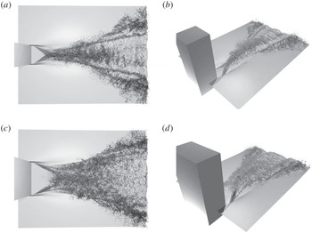
Instantaneous isosurface of volume fraction
 $f=0.5$
for case A (a,b) and C (c,d) within the interrogation domain. Flow is from left to right (
 $+x$
). (a,c) viewed from above; (b,d) viewed from the side. Surface is rendered partially transparent. Dark regions indicate multivalued surface, spray or entrainment.

Figure 2 shows the instantaneous volume fraction isosurface
 $f=0.5$
for cases A and C. The wake contains three distinct regions (present for all cases considered). The first region contains a large depression behind the dry stern with ridges that rise from the lower corner. These ridges, or converging corner waves (CCW), angle towards the stern centreline. Depending on the value of
 $B/D$
, the CCW impact on the centreline (cases A and B) with physics similar to two impacting jets: entraining some air and generating significant spray; or the CCW fully overturn before arriving at the centreline (case C) entraining air in the CCW region. The rooster tail (RT) forms after the CCW region. The length of the RT decreases with
 $B/D$
and its surface is rough with many fine-scale ligaments and spray. The RT region widens to form the beginning of the divergent wave (DW) train behind the stern. Here, the wake surface near the centreline becomes smoother while the edges contain fine structures and quasi-steady breakers. In Part 1, we identify two main scalings of the wake features. First, the wake interface geometry in the CCW region scales ballistically, consistent with supercritical channel expansion flow (Rouse, Bhoota & Hsu Reference Rouse, Bhoota and Hsu1949; Martínez-Legazpi et al.
Reference Martínez-Legazpi, Rodríguez-Rodríguez, Marugán-Cruz and Lasheras2013). Second, the air entrainment characteristics along the extent of the wake scale as
 $\hat{x}=x/Fr$
, consistent with the convective nature of the flow. As the forthcoming analysis focuses on the turbulent nature of the IHVDT, we scale the streamwise component as
 $\hat{x}$
. Using this scaling, we define two different locations along the wake: the location where the converging corner waves collide (or the end of the CCW)
 $\hat{x}_{c}$
; and the start of the DW region defined for convenience as the location where the average wake interface crosses the plane of the half-beam
 $\hat{x}_{B}$
(see table 1 for details).
2.1 IHVDT analysis framework
The best analysis framework for IHVDT is not clear (see e.g. the review in Brocchini & Peregrine Reference Brocchini and Peregrine2001). When one fluid is dispersed throughout the other as is the case for the immiscible flows studied here, conditional phase-weighted averaging is helpful (Drew Reference Drew1983; Aliod & Dopazo Reference Aliod and Dopazo1990; Brocchini & Peregrine Reference Brocchini and Peregrine2001). The framework takes heterogeneous mixed flow and replaces it with a mixture of coexisting equivalent fluids. However, the technique tends to smooth out continuous phase fluctuations caused by the discrete phase (Lance & Bataille Reference Lance and Bataille1991). To assess the nature of IHVDT in its most basic form, we choose an unconditioned temporal averaging with Reynolds decomposition. As such, our notation is the instantaneous velocity field
 $U_{i}(\boldsymbol{x},t)=\overline{U}_{i}(\boldsymbol{x})+u_{i}^{\prime }(\boldsymbol{x},t)$
for
 $i=1\ldots 3$
, with
 $\overline{U}_{i}$
the temporal mean value and
 $u_{i}^{\prime }$
the random centred fluctuation such that
 $\overline{u_{i}^{\prime }\,}=0$
. The other flow quantities are total pressure
 $P=\overline{P}+p^{\prime }$
, density
 $\unicode[STIX]{x1D70C}=\overline{\unicode[STIX]{x1D70C}}+\unicode[STIX]{x1D70C}^{\prime }$
and viscosity
 $\unicode[STIX]{x1D707}=\overline{\unicode[STIX]{x1D707}}+\unicode[STIX]{x1D707}^{\prime }$
. With these definitions, the governing equations for the mean continuity (2.1), momentum (2.2) and kinetic energy (2.3) are
 $$\begin{eqnarray}\displaystyle {\displaystyle \frac{\unicode[STIX]{x2202}\overline{\unicode[STIX]{x1D70C}}}{\unicode[STIX]{x2202}t}}+{\displaystyle \frac{\unicode[STIX]{x2202}\left(\overline{\unicode[STIX]{x1D70C}}\overline{U}_{k}\right)}{\unicode[STIX]{x2202}x_{k}}}=-{\displaystyle \frac{\unicode[STIX]{x2202}\,}{\unicode[STIX]{x2202}x_{k}}}\left(\overline{\unicode[STIX]{x1D70C}u_{k}^{\prime }}\right), & & \displaystyle\end{eqnarray}$$
 $$\begin{eqnarray}\displaystyle & & \displaystyle {\displaystyle \frac{\unicode[STIX]{x2202}\overline{\unicode[STIX]{x1D70C}}\,\overline{U}_{i}}{\unicode[STIX]{x2202}t}}+{\displaystyle \frac{\unicode[STIX]{x2202}\left(\overline{\unicode[STIX]{x1D70C}}\,\overline{U}_{i}\,\overline{U}_{j}\right)}{\unicode[STIX]{x2202}x_{j}}}={\displaystyle \frac{\overline{\unicode[STIX]{x1D70C}}}{Fr^{2}}}g_{i}-{\displaystyle \frac{\unicode[STIX]{x2202}\overline{P}}{\unicode[STIX]{x2202}x_{i}}}-{\displaystyle \frac{\unicode[STIX]{x2202}\overline{\unicode[STIX]{x1D70C}u_{i}^{\prime }u_{j}^{\prime }}}{\unicode[STIX]{x2202}x_{j}}}+{\displaystyle \frac{\unicode[STIX]{x2202}\overline{\unicode[STIX]{x1D70F}}_{ij}}{\unicode[STIX]{x2202}x_{j}}}-A_{i},\nonumber\\ \displaystyle & & \displaystyle \qquad \text{where}\quad A_{i}={\displaystyle \frac{\unicode[STIX]{x2202}\overline{\unicode[STIX]{x1D70C}u_{i}^{\prime }}}{\unicode[STIX]{x2202}t}}+{\displaystyle \frac{\unicode[STIX]{x2202}}{\unicode[STIX]{x2202}x_{j}}}\left(\overline{\unicode[STIX]{x1D70C}u_{i}^{\prime }}\,\overline{U}_{j}+\overline{\unicode[STIX]{x1D70C}u_{j}^{\prime }}\,\overline{U}_{i}\right)\end{eqnarray}$$
and
 $$\begin{eqnarray}\displaystyle & & \displaystyle {\displaystyle \frac{\unicode[STIX]{x2202}\left(\frac{1}{2}\overline{\unicode[STIX]{x1D70C}}\,\overline{U}_{i}\,\overline{U}_{i}\right)}{\unicode[STIX]{x2202}t}}+{\displaystyle \frac{\unicode[STIX]{x2202}\left[\left(\frac{1}{2}\overline{\unicode[STIX]{x1D70C}}\,\overline{U}_{i}\,\overline{U}_{i}\right)\overline{U}_{j}\right]}{\unicode[STIX]{x2202}x_{j}}}={\displaystyle \frac{\overline{\unicode[STIX]{x1D70C}}\,\overline{U}_{i}}{Fr^{2}}}g_{i}-{\displaystyle \frac{\unicode[STIX]{x2202}\overline{P}\,\overline{U}_{i}}{\unicode[STIX]{x2202}x_{i}}}-A_{i}\overline{U}_{i}\nonumber\\ \displaystyle & & \displaystyle \qquad -\,{\displaystyle \frac{\unicode[STIX]{x2202}\left(\overline{\unicode[STIX]{x1D70C}u_{i}^{\prime }u_{j}^{\prime }}\,\overline{U}_{i}\right)}{\unicode[STIX]{x2202}x_{j}}}+\overline{\unicode[STIX]{x1D70C}u_{i}^{\prime }u_{j}^{\prime }}{\displaystyle \frac{\unicode[STIX]{x2202}\overline{U}_{i}}{\unicode[STIX]{x2202}x_{j}}}+{\displaystyle \frac{\unicode[STIX]{x2202}\left(\overline{\unicode[STIX]{x1D70F}}_{ij}\,\overline{U}_{i}\right)}{\unicode[STIX]{x2202}x_{j}}}-\overline{\unicode[STIX]{x1D70F}}_{ij}{\displaystyle \frac{\unicode[STIX]{x2202}\overline{U}_{i}}{\unicode[STIX]{x2202}x_{j}}}.\end{eqnarray}$$
In the mean governing equations,
 $\unicode[STIX]{x1D70F}_{ij}=\unicode[STIX]{x1D707}\frac{1}{2}(U_{i,j}+U_{j,i})/\mathit{Re}$
is the instantaneous viscous stress tensor and
 $g_{i}=-\unicode[STIX]{x1D6FF}_{i3}$
is the gravitational force. When written in this form, the different contributions of the turbulent mass flux (
 $\overline{\unicode[STIX]{x1D70C}u_{i}^{\prime }}$
) are explicit: (i) the source term on the right-hand side of (2.1); (ii) the
 $A_{i}$
term in (2.2); and (iii) the
 $A_{i}\,\overline{U}_{i}$
term in (2.3). In addition to understanding the overall turbulence characteristics in the mixed-phase region of the transom stern wake, we focus on investigating the relative importance of these TMF terms for IHVDT closure modelling. For completeness, we briefly discuss the use and implications of mass-weighted (or Favre) averaging in appendix C.
We average each case over a quasi-steady time period of
 $t=UT/D=40$
with a sampling rate of
 $\text{d}t=0.01$
, or 4000 samples. We estimate the statistical error in the mean velocity, density, r.m.s. velocity and density fluctuations, turbulent mass flux
 $\overline{\unicode[STIX]{x1D70C}u_{i}^{\prime }}$
and Reynolds stresses
 $\overline{\unicode[STIX]{x1D70C}u_{i}^{\prime }u_{j}^{\prime }}$
, using standard deviations of the entire sample time and multiple sub-time blocks of the simulation, to obtain 95 % confidence in these mean quantities (Friedberg & Cameron Reference Friedberg and Cameron1970; Morales, Nuevo & Rull Reference Morales, Nuevo and Rull1990). The maximum statistical error for all quantities considered is
 $\pm 5.3$
%.
2.2 Definition of the mixed-phase region
 ${\mathcal{R}}$
and conditioning averaged quantities

We define the mixed-phase region
 ${\mathcal{R}}$
to be the variable density region where the average density satisfies
 $\unicode[STIX]{x0394}\overline{\unicode[STIX]{x1D70C}}\leqslant \overline{\unicode[STIX]{x1D70C}}\leqslant 1-\unicode[STIX]{x0394}\overline{\unicode[STIX]{x1D70C}}$
, where the boundary width
 $\unicode[STIX]{x0394}\overline{\unicode[STIX]{x1D70C}}$
is an unknown parameter. We choose the value of
 $\unicode[STIX]{x0394}\overline{\unicode[STIX]{x1D70C}}$
such that
 ${\mathcal{R}}$
: (i) contains much of the relevant quantities such as turbulent kinetic energy and turbulent mass flux; (ii) is well behaved; and (iii) does not contain noise generated by individual entrainment or spray events (caused by the 1000:1 water-to-air density ratio). Note that when defined in this manner and combined with the unconditioned time average,
 ${\mathcal{R}}$
includes surface fluctuations as well as entrained air and spray (see figure 1).
As the higher density water motion can have a significant influence on
 $\overline{\unicode[STIX]{x1D70C}u_{i}^{\prime }}$
, we perform a careful statistical analysis to determine
 $\unicode[STIX]{x0394}\overline{\unicode[STIX]{x1D70C}}$
. The full analysis in appendix A shows that
 $\unicode[STIX]{x0394}\overline{\unicode[STIX]{x1D70C}}=0.05$
allows for comparable contributions around the mean interface. Appendix A also contains the definitions of the conditional moments and conditioned averages for the flow. Unless specified, quantities plotted in the forthcoming sections are depth-conditioned averages (A 2) at a location
 $(x,y)$
or area-conditioned (A 3) at a location
 $x$
.
2.3 Mean flow properties within the mixed-phase region in the wake
Figure 3(a) shows transverse (
 $y$
–
 $z$
plane) cuts of
 $\overline{\unicode[STIX]{x1D70C}}$
and
 ${\mathcal{R}}$
in the wake at successive streamwise
 $x$
locations. The pockets of entrained air are visible at the locations of quasi-steady wave breaking in the converging-corner-wave and diverging-wave regions. The surface fluctuations and spray areas above the mean interface
 $\overline{\unicode[STIX]{x1D70C}}=0.5$
are also evident. Generally, at each wake location the
 $z$
extent of
 ${\mathcal{R}}$
is directly related to the breaking and spray formation. When associated only with surface fluctuations, the
 $z$
extent of
 ${\mathcal{R}}$
is small. Figure 3(b) shows
 $S^{{\mathcal{R}}}$
(see (A 3) for notation) along the wake for all three cases. Cases A and B are very similar and case C contains the largest mixed-phase region. The scaling of the mixed-phase region along the wake with
 $Fr$
is consistent with the convective nature of the flow at these ship speeds.
Transverse cuts of (a)
 $\overline{\unicode[STIX]{x1D70C}}$
for case C and (b) conditioned transverse area
 $S^{{\mathcal{R}}}$
for


Figure 4 shows the conditioned mean velocity for all three cases at two
 $\hat{x}$
locations (transverse cuts) and along the wake (streamwise). In the rooster-tail region
 $\hat{x}<\hat{x}_{B}$
(figure 4
a,d,g), the velocity profiles collapse with beam scaling, consistent with the ballistic behaviour identified in Part 1. The wake deficit magnitude
 $U-\overline{U}_{1}$
is proportional to
 $B$
. The magnitudes of the transverse and vertical velocities exhibit no distinct scaling with geometry at this location. We note here that there exists some asymmetry with
 $y$
in the mean velocity profiles (most notably case A e.g. figure 4
h) and r.m.s. fluctuations in figure 5, which we hypothesize are a function of a buffer domain boundary rather than physical phenomenon or a function of statistical convergence.
Values of
 $\langle {\overline{U}_{i}}^{{\mathcal{R}}}\rangle _{z}$
and
 $\langle {\overline{U}_{i}}^{{\mathcal{R}}}\rangle _{yz}$
for


 $\hat{x}=1.5$
; (b,e,h) transverse cut
 $\hat{x}=4.0$
; and (c,f,i) along the wake.

In the diverging-wave region
 $\hat{x}>\hat{x}_{B}$
(figure 4
b,e,h), the wake deficit magnitude peaks on the outer boundaries of
 ${\mathcal{R}}$
, decreases and then increases again on the centreline
 $y/B=0$
. This is in direct contrast with the general transverse spreading of the wake deficit observed in bluff-body wakes (Pope Reference Pope2000) due to the presence of the breaking waves on the outer boundaries of
 ${\mathcal{R}}$
. When we consider the aggregate plot along the wake (see figure 4
c,f,i), we see that the streamwise and transverse velocities show no significant dependence on geometry. However, the vertical velocity shows an inverse relationship with
 $B$
, in particular near
 $\hat{x}=1$
. This is due to the presence of the converging corner waves as identified in Part 1. This location represents (for cases A and B) where the converging jets collide on the centreline, generating a large vertical velocity. For case C, the converging corner waves break near
 $\hat{x}\approx 0.5$
. Thus, the converging jets are weaker at
 $\hat{x}\approx 1$
generating a decreased vertical velocity.
3 Turbulence characteristics within the mixed-phase region
The three geometries in this study do have physical differences in the mean interface characteristics (see §§ 2.3 and 4 of Part 1). However, with the definition of
 ${\mathcal{R}}$
and the use of the conditioning outlined in § 2.2, the three cases have many similarities in terms of their turbulent statistics. The following section discusses the turbulent characteristics in
 ${\mathcal{R}}$
for case A. We include the other cases only when it warrants identifying significant differences or similarities.
3.1 Root mean square fluctuations
Figure 5 plots transverse cuts of the r.m.s. velocity
 $u_{i}^{rms}=\sqrt{\overline{u_{i}^{^{\prime }2}}}$
and r.m.s. density fluctuations
 $\unicode[STIX]{x1D70C}^{rms}$
. Generally, the transverse cuts across the rooster tail (figure 5
a) contain a near-homogeneous behaviour within
 $|y/B|\leqslant 1$
for velocity components and peak at the centreline for the density components. Transversely across the diverging wave (figure 5
b), the fluctuations have peaks at
 $|y/B|\sim 3$
(caused by the quasi-steady breaking waves) that frame a near-homogeneous behaviour within
 $|y/B|<2$
. Along the wake (see figure 5
c), all of the fluctuations peak near
 $\hat{x}=1$
. The rooster-tail region
 $1<\hat{x}<\hat{x}_{B}$
shows near constant density fluctuations with a decrease in the velocity fluctuations. In the diverging-wave region
 $\hat{x}>\hat{x}_{B}$
both density and velocity fluctuations increase due to the presence of breaking waves. There exists a subtle difference in the magnitudes of the velocity fluctuations (both transversely and along the entire wake) implying a degree of anisotropy.
Root mean square velocity and density fluctuations. (a) Transverse cut at
 $\hat{x}=1.5$
; (b) transverse cut at
 $\hat{x}=4.0$
; (c) along the wake.

 $u_{1}^{rms}$
;

 $u_{2}^{rms}$
;

 $u_{3}^{rms}$
; and ○
 $\unicode[STIX]{x1D70C}^{rms}$
. Vertical

 $\hat{x}_{c}$
and
 $\hat{x}_{B}$
, respectively. Data are case A.

3.2 IHVDT anisotropy
Figure 6 shows the IHVDT Reynolds stress
 $\unicode[STIX]{x1D70E}_{ij}=\overline{\unicode[STIX]{x1D70C}u_{i}^{\prime }u_{j}^{\prime }}$
and the anisotropy tensor components
 $\unicode[STIX]{x1D623}_{ij}=\unicode[STIX]{x1D622}_{ij}/2k=\unicode[STIX]{x1D70E}_{ij}/2k-1/3\unicode[STIX]{x1D6FF}_{ij}$
along the wake (here
 $\unicode[STIX]{x1D622}_{ij}=\unicode[STIX]{x1D70E}_{ij}-2/3k\unicode[STIX]{x1D6FF}_{ij};k=1/2\overline{\unicode[STIX]{x1D70C}u_{i}^{\prime }u_{i}^{\prime }}$
). The diagonal components of the Reynolds stresses are negative and peak near
 $\hat{x}_{c}$
. The magnitude decreases in the rooster tail and then increases again in the diverging-breaking-wave region
 $\hat{x}>\hat{x}_{B}$
. The diagonal components of the anisotropy tensor (see figure 6
c) show that only the transverse and vertical components of the velocity fluctuations contribute to the turbulent kinetic energy (TKE) immediately off of the stern (
 $\unicode[STIX]{x1D623}_{22}>0$
and
 $\unicode[STIX]{x1D623}_{33}>0$
at
 $\hat{x}\gtrsim 0$
). The streamwise component quickly becomes dominant
 $0.25<\hat{x}<\hat{x}_{c}$
and the energy is in both the streamwise and transverse directions near
 $\hat{x}_{c}$
. The transverse and vertical components exchange relative importance in the rooster tail (
 $\unicode[STIX]{x1D623}_{11}>\unicode[STIX]{x1D623}_{33}\sim 0$
and
 $\unicode[STIX]{x1D623}_{22}<0$
). This reverses itself further downstream in the diverging-wave region (
 $\unicode[STIX]{x1D623}_{11}>\unicode[STIX]{x1D623}_{22}\sim 0$
and
 $\unicode[STIX]{x1D623}_{33}<0$
). The off-diagonal terms of the Reynolds-stress tensor (figure 6
b) are an order of magnitude smaller than their diagonal counterparts. Figure 6(d) shows
 $\unicode[STIX]{x1D623}_{13}$
to be the most significant anisotropy tensor term along the entire wake.
Reynolds-stress tensor
 $\unicode[STIX]{x1D70E}_{ij}=\overline{\unicode[STIX]{x1D70C}u_{i}^{\prime }u_{j}^{\prime }}$
and anisotropy tensor
 $\unicode[STIX]{x1D623}_{ij}$
along the wake. (a) Diagonal components
 $\unicode[STIX]{x1D70E}_{ii}$
:

 $\unicode[STIX]{x1D70E}_{11}$
;

 $\unicode[STIX]{x1D70E}_{22}$
; and

 $\unicode[STIX]{x1D70E}_{33}$
. (b) Off-diagonal components
 $\unicode[STIX]{x1D70E}_{ij\,i\neq j}$
:

 $\unicode[STIX]{x1D70E}_{12}$
;

 $\unicode[STIX]{x1D70E}_{13}$
; and

 $\unicode[STIX]{x1D70E}_{23}$
. (c) Diagonal components
 $\unicode[STIX]{x1D623}_{ii}$
:

 $\unicode[STIX]{x1D623}_{11}$
;

 $\unicode[STIX]{x1D623}_{22}$
; and

 $\unicode[STIX]{x1D623}_{33}$
. (b) Off-diagonal components
 $\unicode[STIX]{x1D623}_{ij\,i\neq j}$
:

 $\unicode[STIX]{x1D623}_{12}$
;

 $\unicode[STIX]{x1D623}_{13}$
; and

 $\unicode[STIX]{x1D623}_{23}$
. Vertical

 $\hat{x}_{c}$
and
 $\hat{x}_{B}$
, respectively. Data are case A.

A measure of the flow isotropy from the invariants of the anisotropy tensor (
 $I=\unicode[STIX]{x1D623}_{ii}$
;
 $II=\unicode[STIX]{x1D623}_{ij}\unicode[STIX]{x1D623}_{ji}$
;
 $III=\unicode[STIX]{x1D623}_{ij}\unicode[STIX]{x1D623}_{jk}\unicode[STIX]{x1D623}_{ki}$
) is the two-dimensionality or anisotropy parameter
 ${\mathcal{J}}=1{-}9(1/2II{-}III)$
, where
 ${\mathcal{J}}=0$
is highly anisotropic and
 ${\mathcal{J}}=1$
is isotropic (Jovanovic Reference Jovanovic2004). In the rooster tail (figure 7
a), the flow is moderately isotropic on the wake centreline, reaching a value of 0.6–0.8. However, it is highly anisotropic at
 $|y/B|\approx 1$
with a secondary peak value of 0.4 for
 $y/B>1$
. In the diverging-wave region (figure 7
b), the area of moderately isotropic behaviour widens with the wake width. However, the area of increased anisotropy (while not as strong) still persists at
 $|y/B|\sim 1$
and
 $|y/B|\sim 4$
. Figure 7(c) shows the aggregate anisotropy parameter plotted along the wake for all three cases. The flow generally changes from highly anisotropic to moderately isotropic downstream with a general collapse of all cases in the far wake to a similar value of
 ${\mathcal{J}}\approx 0.6$
. The flow never achieves fully isotropic behaviour within
 $O(10)D$
behind the stern.
Anisotropy parameter
 ${\mathcal{J}}$
. (a) Case A transverse cut
 $\hat{x}=1.5$
; (b) case A transverse cut
 $\hat{x}=4.0$
; and (c) along the wake for


The method of componentality contours (Emory & Iaccarino Reference Emory and Iaccarino2014) provides a technique of visualizing the anisotropy of complex flows similar to the anisotropy invariant map (Lumley & Newman Reference Lumley and Newman1977) and barycentric map (Banerjee et al.
Reference Banerjee, Krahl, Durst and Zenger2007) based on the invariants and their eigenvalues
 $\unicode[STIX]{x1D706}_{i}$
. The componentality contours construct a colour map from the barycentric coordinates
 $$\begin{eqnarray}\displaystyle x_{B}=C_{1c}+{\textstyle \frac{1}{2}}C_{3c},\quad y_{B}=C_{3c};\quad \text{with}\quad C_{1c}=\unicode[STIX]{x1D706}_{1}-\unicode[STIX]{x1D706}_{2}\quad \text{and}\quad C_{3c}=3\unicode[STIX]{x1D706}_{3}+1,\qquad & & \displaystyle\end{eqnarray}$$
where
 $\unicode[STIX]{x1D706}_{i}$
is defined such that
 $\unicode[STIX]{x1D706}_{1}\geqslant \unicode[STIX]{x1D706}_{2}\geqslant \unicode[STIX]{x1D706}_{3}$
. Note here that the Euclidean domain mapping chosen by Banerjee et al. (Reference Banerjee, Krahl, Durst and Zenger2007) simplifies such that
 $C_{2c}=2(\unicode[STIX]{x1D706}_{2}-\unicode[STIX]{x1D706}_{3})$
is not necessary for these definitions. The colour map translates
 $C_{n}$
,
 $n=(1c,2c,3c)$
to RGB (red green blue) colour components for visualization
 $$\begin{eqnarray}\displaystyle [R~G~B]^{\text{T}}=C_{1c}[1~0~0]^{\text{T}}+C_{2c}[0~1~0]^{\text{T}}+C_{3c}[0~0~1]^{\text{T}} & & \displaystyle\end{eqnarray}$$
(for further colour map details see Emory & Iaccarino Reference Emory and Iaccarino2014). Overlaying the colour map onto flows of geometric complexity provides a powerful tool for identifying local regions of anisotropy.
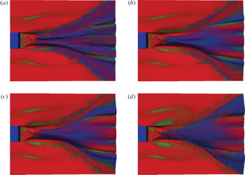
Figures 8 and 9 show the componentality contours in the wake of the stern. As shown in the legend in figure 9(a), red represents 1-component turbulence
 $x_{1C}$
, green 2-component turbulence
 $x_{2C}$
and blue 3-component turbulence
 $x_{3C}$
. Outside of the mixed-phase region (see figure 9), the mainly 1-component bulk water turbulence becomes 2-component and isotropic in the diverging-wave region. The spreading wake of the geometry in the bulk air turbulence is also visible. Within the mixed-phase region, the converging corner waves inject 1-component turbulent flow into the rooster-tail region (see figures 8 and 9
b). The rooster-tail centreline at
 $\hat{x}_{c}$
(figure 9
b) as well as the scars formed by the breaking waves in the diverging-wave region (figure 9
c) are sources of 2-component turbulence in
 ${\mathcal{R}}$
. Also shown in figure 9(c), is that the wave breaking draws 1-component bulk water turbulence up into
 ${\mathcal{R}}$
.
Componentality contours on
 $\overline{\unicode[STIX]{x1D70C}}$
isosurfaces. (a)
 $\overline{\unicode[STIX]{x1D70C}}=0.95$
; (b)
 $\overline{\unicode[STIX]{x1D70C}}=0.75$
; (c)
 $\overline{\unicode[STIX]{x1D70C}}=0.25$
; (d)
 $\overline{\unicode[STIX]{x1D70C}}=0.05$
. Data are case A. See figure 9(a) for legend.

Componentality contours at transverse locations. Data are case A. (a) Legend; (b)
 $\hat{x}=1.4$
; (c)
 $\hat{x}=3.9$
. In each image, upper white line is
 $\overline{\unicode[STIX]{x1D70C}}=0.05$
, lower white line
 $\overline{\unicode[STIX]{x1D70C}}=0.95$
.

3.3 Turbulent kinetic energy
Figure 10(a) shows the mean turbulent kinetic energy
 $k=\frac{1}{2}\overline{\unicode[STIX]{x1D70C}u_{i}^{\prime }u_{i}^{\prime }}$
along the wake for all three cases. The initial peak of the TKE occurs at
 $\hat{x}\sim 1$
, as expected. For case C, there are two peaks in the CCW, the first at
 $\hat{x}\sim 0.5$
and then at
 $\hat{x}_{c}$
. This is due to the fact that the converging corner waves break prior to the collision point for this case. The TKE decreases in the rooster tail and then increases again in the diverging-wave region. Cases B and C have an additional local peak at
 $\hat{x}\sim 2.75$
.
The mean turbulent kinetic energy obeys the exact transport equation in variable density flows (Chassaing et al. Reference Chassaing, Antonia, Anselmet, Joly and Sarkar2002)
 $$\begin{eqnarray}\displaystyle {\displaystyle \frac{\unicode[STIX]{x2202}k}{\unicode[STIX]{x2202}t}}+{\displaystyle \frac{\unicode[STIX]{x2202}(k\overline{U}_{j})}{\unicode[STIX]{x2202}x_{j}}} & = & \displaystyle -{\displaystyle \frac{\unicode[STIX]{x2202}\left(\frac{1}{2}\overline{\unicode[STIX]{x1D70C}u_{i}^{\prime }u_{i}^{\prime }u_{j}^{\prime }}\right)}{\unicode[STIX]{x2202}x_{j}}}-\underbrace{\overline{\unicode[STIX]{x1D70C}u_{i}^{\prime }u_{j}^{\prime }}{\displaystyle \frac{\unicode[STIX]{x2202}\overline{U}_{i}}{\unicode[STIX]{x2202}x_{j}}}}_{\text{a}}+\underbrace{{\displaystyle \frac{\overline{\unicode[STIX]{x1D70C}u_{i}^{\prime }}}{Fr^{2}}}g_{i}}_{\text{b}}\nonumber\\ \displaystyle & & \displaystyle -\,{\displaystyle \frac{\unicode[STIX]{x2202}\overline{p^{\prime }u_{i}^{\prime }}}{\unicode[STIX]{x2202}x_{i}}}+\overline{p^{\prime }{\displaystyle \frac{\unicode[STIX]{x2202}u_{i}^{\prime }}{\unicode[STIX]{x2202}x_{i}}}}+{\displaystyle \frac{\unicode[STIX]{x2202}\overline{\unicode[STIX]{x1D70F}_{ij}^{\prime }u_{i}^{\prime }}}{\unicode[STIX]{x2202}x_{j}}}-\overline{\unicode[STIX]{x1D70F}_{ij}^{\prime }{\displaystyle \frac{\unicode[STIX]{x2202}u_{i}^{\prime }}{\unicode[STIX]{x2202}x_{j}}}}-\underbrace{\overline{\unicode[STIX]{x1D70C}u_{i}^{\prime }}\left({\displaystyle \frac{\unicode[STIX]{x2202}\overline{U}_{i}}{\unicode[STIX]{x2202}t}}+\overline{U}_{j}{\displaystyle \frac{\unicode[STIX]{x2202}\overline{U}_{i}}{\unicode[STIX]{x2202}x_{j}}}\right)}_{\text{c}}.\qquad\end{eqnarray}$$
Equation (3.3) does not include the effect of surface tension which is not included in the iLES. Dodd & Ferrante (Reference Dodd and Ferrante2016) established that the power of surface tension can act either as a source or sink of TKE, and that for turbulent
 $We<5$
, the change of the surface energy on the droplet due to droplet oscillation and coalescence can be significant and any increase in TKE energy is irreversibly lost to viscous dissipation. Thus, bubbles with small turbulent Weber number will impact turbulent dissipation of the carrier fluid and should be incorporated in any explicit sub-grid-scale turbulence model. However, as the smallest bubbles we resolve have
 $We$
several orders of magnitude greater than this critical value, the TKE analyses presented here do not account for such effects.
Figure 10(b) shows the terms of (3.3) for case A. To determine a best estimate of the turbulent dissipation for this iLES, we calculate
 $\overline{\unicode[STIX]{x1D70F}_{ij}^{\prime }\unicode[STIX]{x2202}u_{i}^{\prime }/\unicode[STIX]{x2202}x_{j}}$
and scale it by
 $\unicode[STIX]{x1D708}_{e}^{-1}$
value from table 1. We apply the same scaling to the viscous transport term
 $\unicode[STIX]{x2202}\overline{\unicode[STIX]{x1D70F}_{ij}^{\prime }u_{i}^{\prime }}/\unicode[STIX]{x2202}x_{j}$
. The production by mean shear and turbulent dissipation peaks near
 $\hat{x}_{c}$
. The transport terms are also significant in the converging-corner-wave region, as expected. Further downstream, the production by mean shear and turbulent dissipation are the dominant terms. However, the convection and transport terms continue to make small contributions in this region.
(a) Mean turbulent kinetic energy
 $k$
along the wake for


 $\hat{x}_{c}$
and
 $\hat{x}_{B}$
, respectively.

The terms directly associated with the variable density turbulent flows are terms b and c – as they explicitly involve the turbulent mass flux
 $\overline{\unicode[STIX]{x1D70C}u_{i}^{\prime }}$
. We define the production of IHVDT turbulence
 ${\mathcal{P}}$
as the sum of that due to traditional production by the mean velocity gradients (term a) and the TMF terms b and c of (3.3). Thus,
 $$\begin{eqnarray}\displaystyle {\mathcal{P}}=\overline{\unicode[STIX]{x1D70C}}~\overline{u_{i}^{\prime }u_{j}^{\prime }}{\displaystyle \frac{\unicode[STIX]{x2202}\overline{U}_{i}}{\unicode[STIX]{x2202}x_{j}}}+\overline{\unicode[STIX]{x1D70C}^{\prime }u_{i}^{\prime }u_{j}^{\prime }}{\displaystyle \frac{\unicode[STIX]{x2202}\overline{U}_{i}}{\unicode[STIX]{x2202}x_{j}}}-\overline{\unicode[STIX]{x1D70C}u_{i}^{\prime }}\left({\displaystyle \frac{\unicode[STIX]{x2202}\overline{U}_{i}}{\unicode[STIX]{x2202}t}}+\overline{U}_{j}{\displaystyle \frac{\unicode[STIX]{x2202}\overline{U}_{i}}{\unicode[STIX]{x2202}x_{j}}}\right)+{\displaystyle \frac{\overline{\unicode[STIX]{x1D70C}u_{i}^{\prime }}}{Fr^{2}}}g_{i}. & & \displaystyle\end{eqnarray}$$
The first two terms arise from decomposing the density into its mean and average components in term a of (3.3).
Figure 11 shows the total production of TKE and its sub-components along the wake for case A and C, respectively. For case A, production due to mean shear and mean density
 ${\mathcal{P}}_{1}$
is responsible for most of the TKE production in the converging corner waves. The production from mean shear with variable density
 ${\mathcal{P}}_{2}$
and gravity effects
 ${\mathcal{P}}_{4}$
provides the rest of the production in this region, and
 ${\mathcal{P}}_{3}$
actually decreases the total TKE production moderately. For the case where the waves break within the converging-corner-wave region (case C), the gravity effects are as important (if not more) than the production by mean shear
 ${\mathcal{P}}_{1}+{\mathcal{P}}_{2}$
. For both case A and case C, the local peak of TKE at
 $\hat{x}\sim 2.75$
corresponds to a peak in the TMF specific term
 ${\mathcal{P}}_{3}$
and the mean shear term
 ${\mathcal{P}}_{1}$
.
Value of
 ${\mathcal{P}}$
and its sub-components
 ${\mathcal{P}}_{i},i=1\ldots 4$
for (a) case A and (b) case C.

 ${\mathcal{P}}$
;

 ${\mathcal{P}}_{1}$
;

 ${\mathcal{P}}_{2}$
;

 ${\mathcal{P}}_{3}$
; and

 ${\mathcal{P}}_{4}$
. Vertical

 $\hat{x}_{c}$
and
 $\hat{x}_{B}$
from left to right, respectively.

4 Turbulent mass flux effects in IHVDT
We establish a physical interpretation of the Eulerian concept of TMF with the Lagrangian concepts of spray and entrainment. This is accomplished by considering the sign of the TMF. For example, choose a point on the wake deficit profile of figure 4. A positive velocity fluctuation represents a particle ‘moving outward’ and negative represents it ‘moving inward’ on the wake deficit profile. Additionally, a positive density fluctuation infers a passing droplet and negative infers a passing air bubble. If we consider for a moment TMF only due to bubbles:
 $\overline{\unicode[STIX]{x1D70C}u_{i}^{\prime }}>0$
represents an air bubble moving outward on the wake deficit profile – or entrainment and
 $\overline{\unicode[STIX]{x1D70C}u_{i}^{\prime }}<0$
represents the bubble moving into the profile – or detrainment. In the context of spray:
 $\overline{\unicode[STIX]{x1D70C}u_{i}^{\prime }}>0$
implies spray formation and
 $\overline{\unicode[STIX]{x1D70C}u_{i}^{\prime }}<0$
implies drops moving into the wake deficit profile.
Connecting this to the stern wake, figure 12 shows the TMF along the wake for each component. In the streamwise direction (figure 12
a), cases A and B have consistent profiles, with case C containing significantly more positive TMF in the converging-corner-wave region, which is expected for this geometry. The transverse TMF (figure 12
b) peaks in both the RT and DW regions for all three cases. For the vertical TMF (figure 12
c), there are positive peaks in the CCW region due to spray and in the DW due to both spray and entrainment. From (2.1), the divergence of
 $\overline{\unicode[STIX]{x1D70C}u_{i}^{\prime }}$
is a source term for the mean mass conservation equation. In Part 1 (see figure 8), we plot the change in
 $\overline{\unicode[STIX]{x1D70C}}$
along an average streamline in the wake and discuss the TMF source term within this context for cases A and C.
To refine this concept further, figure 13 shows the transverse cut of TMF and the extent of
 ${\mathcal{R}}$
at two locations in the wake for case A. When viewed in this manner, we can see the contributions of the different physical mechanisms to the TMF. For example, the surface fluctuations contribute to the TMF at the outer boundaries of the mixed region as well as the centreline of the wake (e.g. the positive peaks of
 $\overline{\unicode[STIX]{x1D70C}u_{1}^{\prime }}$
at
 $|y/B|\sim 1$
in figure 13(a) and
 $|y/B|<3$
in figure 13(b)). The entrainment contributes at the location of the quasi-steady breaking waves (e.g. the positive peaks of all three components at
 $|y/B|\sim 3$
in figure 13
b).
Turbulent mass flux along the wake for all three cases. (a)
 $\overline{\unicode[STIX]{x1D70C}u_{1}^{\prime }}$
; (b)
 $\overline{\unicode[STIX]{x1D70C}u_{2}^{\prime }}$
; (c)
 $\overline{\unicode[STIX]{x1D70C}u_{3}^{\prime }}$
. For all


Transverse cut of TMF for case A (a)
 $\hat{x}=1.5$
and (b)
 $\hat{x}=4.0$
. For all

 $\overline{\unicode[STIX]{x1D70C}u_{1}^{\prime }}$
;

 $\overline{\unicode[STIX]{x1D70C}u_{2}^{\prime }}$
;

 $\overline{\unicode[STIX]{x1D70C}u_{3}^{\prime }}$
; and

 ${\mathcal{R}}$
.

The Eulerian construct of TMF provides a mechanism to incorporate the combined effects of entrainment, spray and surface fluctuations into a single quantity (e.g. figure 1). In § 3.3, we established its relevance to the production of TKE. As an example of its influence to the mean flow equations, figure 14 compares the forcing from the Reynolds stresses in the mean momentum equations with that of the TMF forcing
 $A_{i}$
of (2.2). For all three mean momentum components, the TMF forcing is of the same magnitude as that of the Reynolds-stress forcing and either contributes or is in direct opposition to this term. For example, in the streamwise direction (figure 14
a), the TMF is in direct opposition to and greater in magnitude than the Reynolds-stress forcing. In the transverse direction (figure 14
b), the TMF generally adds to the Reynolds-stress forcing throughout the wake and is the greater of the two contributions to the mean momentum in the diverging-wave region. Figure 14(c) shows that the vertical component of the TMF to be a factor of two greater than the Reynolds-stress forcing in the CCW region.
Comparison of forcing from Reynolds stresses and TMF in the mean momentum equation. (a)
 $x$
component; (b)
 $y$
component; and (c)
 $z$
component. From (2.2):

 $\unicode[STIX]{x2202}/\unicode[STIX]{x2202}x_{j}(\overline{\unicode[STIX]{x1D70C}u_{i}^{\prime }u_{j}^{\prime }})$
and

 $A_{i}$
. Vertical

 $\hat{x}_{c}$
and
 $\hat{x}_{B}$
from left to right, respectively. Data are case A.

The results of §§ 3 and 4 show that: (i) the IHVDT in the mixed-phase region
 ${\mathcal{R}}$
is anisotropic; (ii) the location of the anisotropy in
 ${\mathcal{R}}$
qualitatively correlates with highly localized TMF; and (iii) TMF makes a contribution to the production of TKE and is of comparable magnitude to that of the Reynolds-stress forcing in the mean momentum equations. These three findings have immediate implications for IHVDT modelling. There are many workshops dedicated to assessing numerical ship hydrodynamics and effective closure schemes for single phase flows (Ratcliffe Reference Ratcliffe1998; Larsson, Stern & Visonneau Reference Larsson, Stern and Visonneau2013) as well as a body of work addressing closure schemes for wake flows with anisotropic behaviour starting with Sotiropoulos & Patel (Reference Sotiropoulos and Patel1995). Therefore, we focus on closure for TMF for IHVDT with the understanding that this is a useful avenue towards modelling multiple physical mechanisms through a single quantity that plays a role in all of the governing equations.
5 Development of TMF closure models
Turbulent scalar fluxes appear within the following different physical contexts: (i) incompressible, variable density mixing flows; (ii) incompressible thermal flows; (iii) passive scalars and (iv) compressible flows at low and high Mach numbers. The modelling of turbulent scalar fluxes remains an active area of research. Algebraic scalar-flux modelling, or first-order methods, connect the scalar fluxes to mean flow quantities (via a linear or nonlinear scheme that incorporates physical mechanisms) (Daly & Harlow Reference Daly and Harlow1970; Sarkar & Lakshmanan Reference Sarkar and Lakshmanan1991; Wei, Zhang & Zhou Reference Wei, Zhang and Zhou2004; Younis, Speziale & Clark Reference Younis, Speziale and Clark2005). Transport models of the scalar fluxes (and variances) predict the flux from an idealized form of the exact scalar flux budget (Launder Reference Launder and Bradshaw1975; Taulbee & VanOsdol Reference Taulbee and VanOsdol1991; Yoshizawa et al. Reference Yoshizawa, Liou, Yokoi and Shih1997; Duranti & Pittaluga Reference Duranti and Pittaluga2000). The goal of both types of closure paradigms is to predict the influence of the turbulent scalar fluxes on the mean (velocity and scalar) flow. Employing transport models introduces the computational cost of additional transport equations (generally three for the scalar flux vector and one for the scalar variance). These equations have terms that require closure (which are also an active area of research). Despite this cost and the additional modelling effort, the transport model paradigm has successfully predicted a range of physical turbulent variable density/scalar problems. As yet, none of the existing TMF closure models – within either paradigm – address IHVDT. As a first step, we begin with the simpler algebraic model framework. The localized nature of the TMF within the wake structure implies that, if successful, an explicit TMF closure model would be computationally expedient over TMF transport equations. The forthcoming results will determine the general validity of the underlying assumptions and the usefulness of the resulting model.
We construct an explicit algebraic relation for
 $\overline{\unicode[STIX]{x1D70C}u_{i}^{\prime }}$
based on a functional method (Younis et al.
Reference Younis, Speziale and Clark2005). We assume that the density is a passive scalar due to the high density ratio and convective nature of the flow and form a functional relationship derived with guidance from the exact form of the TMF transport equations. To retain the explicit nature of the model, we assume that the length and time scales are that of the turbulent motions. After performing the linear expansion and further simplification (details in appendix B), the final form is
 $$\begin{eqnarray}\displaystyle & & \displaystyle -\overline{\unicode[STIX]{x1D70C}u_{i}^{\prime }}=C_{1}{\displaystyle \frac{k^{2}}{\unicode[STIX]{x1D716}}}{\displaystyle \frac{\unicode[STIX]{x2202}\overline{\unicode[STIX]{x1D70C}}}{\unicode[STIX]{x2202}x_{i}}}+C_{2}{\displaystyle \frac{k}{\unicode[STIX]{x1D716}}}\overline{u_{i}^{\prime }u_{j}^{\prime }}{\displaystyle \frac{\unicode[STIX]{x2202}\overline{\unicode[STIX]{x1D70C}}}{\unicode[STIX]{x2202}x_{j}}}+C_{3}{\displaystyle \frac{k^{3}}{\unicode[STIX]{x1D716}^{2}}}{\displaystyle \frac{\unicode[STIX]{x2202}\overline{U}_{i}}{\unicode[STIX]{x2202}x_{j}}}{\displaystyle \frac{\unicode[STIX]{x2202}\overline{\unicode[STIX]{x1D70C}}}{\unicode[STIX]{x2202}x_{j}}}+C_{4}{\displaystyle \frac{k^{2}}{\unicode[STIX]{x1D716}^{2}}}\left(\overline{u_{i}^{\prime }u_{k}^{\prime }}{\displaystyle \frac{\unicode[STIX]{x2202}\overline{U}_{j}}{\unicode[STIX]{x2202}x_{k}}}+\overline{u_{j}^{\prime }u_{k}^{\prime }}{\displaystyle \frac{\unicode[STIX]{x2202}\overline{U}_{i}}{\unicode[STIX]{x2202}x_{k}}}\right)\nonumber\\ \displaystyle & & \displaystyle \quad \times \,{\displaystyle \frac{\unicode[STIX]{x2202}\overline{\unicode[STIX]{x1D70C}}}{\unicode[STIX]{x2202}x_{j}}}+C_{5}{\displaystyle \frac{k}{\unicode[STIX]{x1D716}}}\overline{\unicode[STIX]{x1D70C}}g_{i}+C_{6}{\displaystyle \frac{\overline{\unicode[STIX]{x1D70C}}}{\unicode[STIX]{x1D716}}}\overline{u_{i}^{\prime }u_{j}^{\prime }}g_{j}+C_{7}{\displaystyle \frac{k^{2}}{\unicode[STIX]{x1D716}^{2}}}\overline{\unicode[STIX]{x1D70C}}{\displaystyle \frac{\unicode[STIX]{x2202}\overline{U}_{i}}{\unicode[STIX]{x2202}x_{j}}}g_{j}+C_{8}\overline{\unicode[STIX]{x1D70C}}{\displaystyle \frac{k}{\unicode[STIX]{x1D716}^{2}}}\left(\overline{u_{i}^{\prime }u_{k}^{\prime }}{\displaystyle \frac{\unicode[STIX]{x2202}\overline{U}_{j}}{\unicode[STIX]{x2202}x_{k}}}+\overline{u_{j}^{\prime }u_{k}^{\prime }}{\displaystyle \frac{\unicode[STIX]{x2202}\overline{U}_{i}}{\unicode[STIX]{x2202}x_{k}}}\right)g_{j}.\nonumber\\ \displaystyle & & \displaystyle\end{eqnarray}$$
Here,
 $C_{n}$
,
 $n=1,\ldots ,8$
can be scalars or vectors. In this general form, the even-numbered coefficients are the anisotropic form of their odd-numbered counterparts. The majority of explicit algebraic turbulent (passive) scalar flux models in the literature are a subset of this general model (Younis et al.
Reference Younis, Speziale and Clark2005):
 $C_{1,2}$
represent the fundamental gradient transport hypothesis (GTH) model (Daly & Harlow Reference Daly and Harlow1970; Sarkar & Lakshmanan Reference Sarkar and Lakshmanan1991);
 $C_{3,4}$
include products of the gradients of the scalar and mean velocity (Dakos & Gibson Reference Dakos and Gibson1987). In particular,
 $C_{4}$
incorporates the rate of production of the Reynolds stresses. Terms
 $C_{5{-}8}$
are the buoyancy equivalent of the density gradient terms. Knowing that the underlying turbulence is anisotropic where TMF exists, we will simplify the model and focus on finding coefficients for only the even-numbered terms in (5.1).
5.1 Model coefficients
Retaining the even-numbered terms of (5.1) creates a general 4 term model for a vector quantity, implying a minimum 12 potential values (assuming a global value will be adequate along the entire wake). Determining the model coefficients is a two-part process. The first part identifies the most relevant terms in the model by calculating a conditioned correlation coefficient at a wake location
 $x$
between the model term (in the absence of
 $C_{n}$
) and a subset of the iLES data within
 ${\mathcal{R}}$
. The second part determines the coefficients using a linear-least squares fit between the relevant model terms and the iLES data.
With the available data, we select the subset of the iLES data to be case A and case B, leaving case C for a priori testing in § 5.2. Note that the estimate for
 $\unicode[STIX]{x1D716}$
is the same as that in § 3.3. Analysis of the conditioned correlation coefficients along the wake yields that a regional model focusing on the near wake and far wake has the best potential for success. For the near-wake region (defined here as including the converging-corner-wave and rooster-tail regions,
 $\hat{x}<\hat{x}_{B}$
), the mean density gradient terms of the model (GTH) best correlate with the iLES data, namely
 $C_{2}$
for the
 $y$
- and
 $z$
-component and
 $C_{4}$
for the
 $x$
-component. Thus, we propose the near-wake explicit algebraic turbulent mass flux model (NW) as
 $$\begin{eqnarray}\displaystyle \left.\begin{array}{@{}c@{}}\overline{\unicode[STIX]{x1D70C}u_{1}^{\prime }}=C_{4}{\displaystyle \frac{k^{2}}{\unicode[STIX]{x1D716}^{2}}}\left(\overline{u_{i}^{\prime }u_{k}^{\prime }}{\displaystyle \frac{\unicode[STIX]{x2202}\overline{U}_{j}}{\unicode[STIX]{x2202}x_{k}}}+\overline{u_{j}^{\prime }u_{k}^{\prime }}{\displaystyle \frac{\unicode[STIX]{x2202}\overline{U}_{i}}{\unicode[STIX]{x2202}x_{k}}}\right){\displaystyle \frac{\unicode[STIX]{x2202}\overline{\unicode[STIX]{x1D70C}}}{\unicode[STIX]{x2202}x_{j}}},\\[12.0pt] \overline{\unicode[STIX]{x1D70C}u_{2}^{\prime }}=C_{2}{\displaystyle \frac{k}{\unicode[STIX]{x1D716}}}\overline{u_{i}^{\prime }u_{j}^{\prime }}{\displaystyle \frac{\unicode[STIX]{x2202}\overline{\unicode[STIX]{x1D70C}}}{\unicode[STIX]{x2202}x_{j}}},\\[12.0pt] \overline{\unicode[STIX]{x1D70C}u_{3}^{\prime }}=C_{2}{\displaystyle \frac{k}{\unicode[STIX]{x1D716}}}\overline{u_{i}^{\prime }u_{j}^{\prime }}{\displaystyle \frac{\unicode[STIX]{x2202}\overline{\unicode[STIX]{x1D70C}}}{\unicode[STIX]{x2202}x_{j}}}.\end{array}\right\} & & \displaystyle\end{eqnarray}$$
All terms in this explicit model take the form: forcing
 $\times$
turbulent diffusivity. For this NW model, the forcing is the mean density gradient. The turbulent diffusivity for the streamwise component is the rate of production of stresses
 ${\sim}\overline{u_{i}^{\prime }u_{k}^{\prime }}(\unicode[STIX]{x2202}\overline{U}_{i}/\unicode[STIX]{x2202}x_{k})$
and for the transverse and vertical components the diffusivity is the actual stresses.
For the far-wake region (defined here as
 $\hat{x}>\hat{x}_{B}$
), both the mean density gradients (
 $C_{2}$
and
 $C_{4}$
) and buoyancy terms (
 $C_{6}$
and
 $C_{8}$
) correlate well and the proposed far-wake model (FW) is
 $$\begin{eqnarray}\displaystyle \left.\begin{array}{@{}l@{}}\overline{\unicode[STIX]{x1D70C}u_{1}^{\prime }}=C_{4}^{1}{\displaystyle \frac{k^{2}}{\unicode[STIX]{x1D716}^{2}}}\left(\overline{u_{i}^{\prime }u_{k}^{\prime }}{\displaystyle \frac{\unicode[STIX]{x2202}\overline{U}_{j}}{\unicode[STIX]{x2202}x_{k}}}+\overline{u_{j}^{\prime }u_{k}^{\prime }}{\displaystyle \frac{\unicode[STIX]{x2202}\overline{U}_{i}}{\unicode[STIX]{x2202}x_{k}}}\right){\displaystyle \frac{\unicode[STIX]{x2202}\overline{\unicode[STIX]{x1D70C}}}{\unicode[STIX]{x2202}x_{j}}}+C_{6}{\displaystyle \frac{\overline{\unicode[STIX]{x1D70C}}}{\unicode[STIX]{x1D716}}}\overline{u_{i}^{\prime }u_{j}^{\prime }}g_{j}\\[12.0pt] \quad \qquad +\,C_{8}^{1}\overline{\unicode[STIX]{x1D70C}}{\displaystyle \frac{k}{\unicode[STIX]{x1D716}^{2}}}\left(\overline{u_{i}^{\prime }u_{k}^{\prime }}{\displaystyle \frac{\unicode[STIX]{x2202}\overline{U}_{j}}{\unicode[STIX]{x2202}x_{k}}}+\overline{u_{j}^{\prime }u_{k}^{\prime }}{\displaystyle \frac{\unicode[STIX]{x2202}\overline{U}_{i}}{\unicode[STIX]{x2202}x_{k}}}\right)g_{j},\\[12.0pt] \overline{\unicode[STIX]{x1D70C}u_{2}^{\prime }}=C_{2}^{2}{\displaystyle \frac{k}{\unicode[STIX]{x1D716}}}\overline{u_{i}^{\prime }u_{j}^{\prime }}{\displaystyle \frac{\unicode[STIX]{x2202}\overline{\unicode[STIX]{x1D70C}}}{\unicode[STIX]{x2202}x_{j}}}+C_{4}^{2}{\displaystyle \frac{k^{2}}{\unicode[STIX]{x1D716}^{2}}}\left(\overline{u_{i}^{\prime }u_{k}^{\prime }}{\displaystyle \frac{\unicode[STIX]{x2202}\overline{U}_{j}}{\unicode[STIX]{x2202}x_{k}}}+\overline{u_{j}^{\prime }u_{k}^{\prime }}{\displaystyle \frac{\unicode[STIX]{x2202}\overline{U}_{i}}{\unicode[STIX]{x2202}x_{k}}}\right){\displaystyle \frac{\unicode[STIX]{x2202}\overline{\unicode[STIX]{x1D70C}}}{\unicode[STIX]{x2202}x_{j}}},\\[12.0pt] \overline{\unicode[STIX]{x1D70C}u_{3}^{\prime }}=C_{2}^{3}{\displaystyle \frac{k}{\unicode[STIX]{x1D716}}}\overline{u_{i}^{\prime }u_{j}^{\prime }}{\displaystyle \frac{\unicode[STIX]{x2202}\overline{\unicode[STIX]{x1D70C}}}{\unicode[STIX]{x2202}x_{j}}}+C_{8}^{3}\overline{\unicode[STIX]{x1D70C}}{\displaystyle \frac{k}{\unicode[STIX]{x1D716}^{2}}}\left(\overline{u_{i}^{\prime }u_{k}^{\prime }}{\displaystyle \frac{\unicode[STIX]{x2202}\overline{U}_{j}}{\unicode[STIX]{x2202}x_{k}}}+\overline{u_{j}^{\prime }u_{k}^{\prime }}{\displaystyle \frac{\unicode[STIX]{x2202}\overline{U}_{i}}{\unicode[STIX]{x2202}x_{k}}}\right)g_{j}.\end{array}\right\} & & \displaystyle\end{eqnarray}$$
The forcing in the FW model still involves mean density gradients and then adds buoyancy effects to the streamwise and vertical components. The turbulent diffusivities of the streamwise component buoyancy effects are the Reynolds stresses and their rate of production. The vertical component turbulent diffusivity is only the rate of production of the stresses. For the transverse component, the FW model only depends on the mean density gradient forcing with turbulent diffusivity coming from both the stresses and their rate of production.
We determine the model coefficients for (5.2) and (5.3) using a linear-least squares fit at each
 $\hat{x}$
where all terms for that model correlate using the subset data cases A and B. We define the transition between the models based on
 $\hat{x}_{B}$
in table 1. We note here that this transition location is currently a value obtained from pre-existing simulation data and determining an appropriate scaling estimate of this location is ongoing work. However, knowing the scaling of the salient features in the wake with only the ship geometry and speed obtained in Part 1 and the convective nature of the flow established in §§ 3–4 suggests an estimate of this transition location to be
 $O(2.5{-}3)Fr$
behind the stern. Table 2 shows the resulting model coefficients.
5.2 Model performance
To assess the feasibility of the model to explicitly predict the TMF from resolved quantities, we perform a priori tests of the NW and FW model. Specifically, we use the iLES data of case C and model coefficients of table 2 to compute the model terms in (5.2) and (5.3). For notation purposes, we will name this the ‘MODEL’.

Figures 15 and 16 show the MODEL prediction of the TMF to the actual iLES data TMF at two transverse locations. The highly localized nature of the TMF is evident in all three components (see figure 15
a,c,e). In general, MODEL does not predict some of the streamwise TMF at the core of the rooster tail (located
 $(y/B,z)\approx (\pm 0.5,0.4)$
in figure 15) and all three components near the quasi-steady wave breaking in the FW (located
 $(y/B,z)\approx (\pm 1.5,-0.2)$
in figure 16). This aside, the explicit model predicts the localization and magnitude extremely well at both wake locations. Table 3 contains the conditioned correlation coefficient
 ${\mathcal{C}}$
and conditioned normalized standard deviation
 $\unicode[STIX]{x1D70E}_{N}$
for the transverse locations in figures 15 and 16. In particular, the model captures the transverse and vertical TMF associated with the surface fluctuations and spray areas in the near-wake region and the streamwise TMF in the far-wake region remarkably well.
Transverse cuts at
 $\hat{x}=2.0$
for TMF of (a,c,e) iLES data and (b,d,f) MODEL prediction. (a,b)
 $\overline{\unicode[STIX]{x1D70C}u_{1}^{\prime }}$
; (c,d)
 $\overline{\unicode[STIX]{x1D70C}u_{2}^{\prime }}$
; (e,f)
 $\overline{\unicode[STIX]{x1D70C}u_{3}^{\prime }}$
. Correlation coefficients and normalized standard deviations in table 3.

Transverse cuts at
 $\hat{x}=4.0$
for TMF of (a,c,e) iLES data and (b,d,f) MODEL prediction. (a,b)
 $\overline{\unicode[STIX]{x1D70C}u_{1}^{\prime }}$
; (c,d)
 $\overline{\unicode[STIX]{x1D70C}u_{2}^{\prime }}$
; (e,f)
 $\overline{\unicode[STIX]{x1D70C}u_{3}^{\prime }}$
. Correlation coefficients and normalized standard deviations in table 3.


Transverse cuts at
 $\hat{x}=1.5$
for depth-integrated
 $\langle \overline{\unicode[STIX]{x1D70C}u_{i}^{\prime }}^{{\mathcal{R}}}\rangle _{z}$
:

 $\overline{\unicode[STIX]{x1D70C}u_{1}^{\prime }}$
; (b)
 $\overline{\unicode[STIX]{x1D70C}u_{2}^{\prime }}$
; (c)
 $\overline{\unicode[STIX]{x1D70C}u_{3}^{\prime }}$
. Every eighth point shown for clarity. Correlation coefficients and normalized standard deviations in table 3.

Figure 17 shows a comparison between the depth-integrated MODEL prediction of TMF and the actual iLES data TMF at another NW transverse location. MODEL predicts TMF magnitude and transverse shape at this location extremely well. It also captures the peaks of the TMF for the streamwise and vertical components. However, it consistently under predicts the streamwise component near the centreline and the general magnitude of the transverse component. Figure 18 shows the same comparison between the depth-integrated MODEL prediction and iLES data of the FW region. MODEL predicts the average behaviour of the TMF and the peaks at the outer edges of the wake
 $|y/B|\sim 1.5$
at this
 $\hat{x}$
. However, it fails to capture the strong peaks of transverse and vertical TMF associated with the scars caused by the breaking waves as observed in figure 16. The correlation coefficients and standard deviations for figures 17 and 18 in table 3 show an overall good performance of the explicit model at these locations.
Transverse cuts at
 $\hat{x}=3.0$
for depth-integrated
 $\langle \overline{\unicode[STIX]{x1D70C}u_{i}^{\prime }}^{{\mathcal{R}}}\rangle _{z}$
:

 $\overline{\unicode[STIX]{x1D70C}u_{1}^{\prime }}$
; (b)
 $\overline{\unicode[STIX]{x1D70C}u_{2}^{\prime }}$
; (c)
 $\overline{\unicode[STIX]{x1D70C}u_{3}^{\prime }}$
. Every eighth point shown for clarity. Correlation coefficients and normalized standard deviations in table 3.

Figure 19 shows the model predictions along the wake in aggregate with the conditioned correlation coefficient
 ${\mathcal{C}}$
. Overall, MODEL predicts the TMF qualitatively and quantitatively well with a few exceptions. The first is the under-prediction of transverse and vertical TMF in the CCW region. This is due to the presence of the fully overturning waves in case C, showing that GTH term in (5.2) fit using datasets without overturning is not sufficient. The second is the under-prediction of the streamwise TMF in the rooster-tail region
 $2\lesssim \hat{x}\lesssim 3$
. This is also due to the poor prediction near the centreline in figure 15(a). In a few regions with poor performance (namely
 $\overline{\unicode[STIX]{x1D70C}u_{1}^{\prime }}$
and
 $\overline{\unicode[STIX]{x1D70C}u_{2}^{\prime }}$
for
 $\hat{x}>\hat{x}_{B}$
and
 $\overline{\unicode[STIX]{x1D70C}u_{3}^{\prime }}$
for
 $\hat{x}<\hat{x}_{B}$
) the conditioned correlation coefficient is high, implying that improving model coefficient in this region will improve the overall performance.
Comparison of MODEL predictions of area-integrated
 $\langle \overline{\unicode[STIX]{x1D70C}u_{i}^{\prime }}^{{\mathcal{R}}}\rangle _{yz}$
along the wake. Lower plot: —— iLES; ○ NW Model;
 $\times$
FW Model; and upper plot: —— conditioned correlation coefficient
 ${\mathcal{C}}$
. (a)
 $\overline{\unicode[STIX]{x1D70C}u_{1}^{\prime }}$
; (b)
 $\overline{\unicode[STIX]{x1D70C}u_{2}^{\prime }}$
; (c)
 $\overline{\unicode[STIX]{x1D70C}u_{3}^{\prime }}$
. Every sixteenth point shown for clarity.

 $\hat{x}_{c}$
and
 $\hat{x}_{B}$
from left to right, respectively.

At this point, one may suggest further refinement of the model by dividing it into additional streamwise regions or using additional iLES datasets to improve the form and estimate of the model coefficients. The main objective of the present modelling process is to show whether or not it is feasible to explicitly predict the TMF in the wake from resolved/known quantities. Overall, our model shows that two main physical effects are directly responsible for much of the TMF in the wake: density gradients and buoyancy effects. With further refinement, explicit algebraic models should have a high potential for success in this type of scalar flux modelling.
6 Summary
We present analysis and modelling of the incompressible highly variable density turbulence of the three-dimensional air entraining flow in the wake of a canonical surface ship for a dry draft-based Froude number
 $Fr=2.53$
and a range of half-beam-to-draft ratios
 $1\leqslant B/D\leqslant 1.77$
. The high-resolution iLES presented in Part 1 (Hendrickson et al.
Reference Hendrickson, Weymouth, Yu and Yue2019) employ state-of-the-art simulation methods cVOF (Weymouth & Yue Reference Weymouth and Yue2010) and BDIM (Weymouth & Yue Reference Weymouth and Yue2011) for robust and accurate prediction of the large-scale flow field and air entrainment for this complex three-dimensional flow. Starting with these datasets, we perform a detailed analysis of the turbulent flow field using an unconditioned Reynolds averaging framework and develop an explicit algebraic closure model for the resulting turbulent mass flux. For the unconditioned average framework, we define the mixed-phase region
 ${\mathcal{R}}$
based on the average density. This enables us to focus solely on the IHVDT region. We define the boundary of the mixed-phase region using statistics of the variable density such that it contains most of the relevant quantities without noise generated by individual entrainment or spray events.
The analyses provide new insight into the behaviour of the mixed-phase region. In particular, in the diverging-wave region, the mixed-phase region is relatively thin (vertically) along the wake centreline and thickens at the edges of the wake where wave breaking occurs. Through the converging-corner-wave and rooster-tail regions, the mixed-phase region extent (and all of the subsequent kinetics, dynamics and turbulence in
 ${\mathcal{R}}$
) scales transversely with the beam. The mean flow in
 ${\mathcal{R}}$
is initially similar to other wake flows with a (wake deficit) peak on the wake centreline. However, unlike typical wake flows where the wake deficit spreads and decreases in magnitude at downstream locations, the stern wake also contains peaks at the transverse edges due to the presence of quasi-steady wave breaking. The draft-based Froude number scales quantities along the wake, consistent with the convective nature of the flow.
Detailed analysis of the turbulence statistics, IHVDT Reynolds stresses and anisotropy tensor shows that the highly anisotropic flow expansion off of the stern regularizes to a moderately anisotropic flow. The energy resides in the transverse and vertical components in the converging-corner-wave region, as should be expected. In the rooster-tail region, the streamwise and vertical components contain the energy, which then returns to the streamwise and transverse components in the diverging-wave region. The flow never achieves a truly isotropic nature within the first
 $O(10D)$
of the stern. Visualization using the componentality contours reveal that the converging corner waves inject 1-component turbulence into the rooster-tail region. The centreline of the rooster tail and the breaking waves in the diverging-wave region introduce 2-component turbulence into the mixed-phase region. Additionally, the wave breaking in the diverging-wave region draws 1-component turbulence from the bulk water region. Thus, quasi-steady wave breaking regions and air entrainment will always introduce anisotropy to the flow.
The converging-corner-wave region contains the peak turbulent kinetic energy. For the geometries where the converging corner waves collide before fully breaking (the two narrowest geometries), this peak location is the collision point
 $\hat{x}_{c}$
. For the widest geometry, the TKE actually peaks twice: once at the location where the converging waves break
 $\hat{x}<\hat{x}_{c}$
and then at
 $\hat{x}_{c}$
. The TKE generally decreases in the rooster tail and then increases in the diverging-wave region. Inspection of the TKE budget shows strong turbulent dissipation with little production in the rooster-tail region, causing the decrease in TKE. Quasi-steady wave breaking causes the increase in TKE in the diverging-wave region. The mean density shear production term produces most of the IHVDT. However, additional contributions come from the gravity-based turbulent mass flux and the variable density shear production. In fact, for the widest geometry, the production by TMF is stronger than that of mean shear for a significant portion of the wake.
Analysis of the turbulent mass flux in the near wake of the stern shows that it is highly localized, peaking in the converging-corner-wave region. It is always significant at the transverse edges of the diverging-wave-region. We show the contributions of TMF to the mean momentum equations are of the same magnitude as that of the IHVDT Reynolds stresses, sometimes in direct opposition to them. Thus, their effect on the mean equations must be accounted for in turbulence closure modelling.
Finally, we investigate the feasibility of constructing a turbulent mass flux closure model in the absence of any dispersed phase model. We construct an anisotropic explicit algebraic turbulent mass flux closure model based on a functional derived from the exact TMF governing equation to predict its effect on the mean flow governing and turbulent kinetic energy equations. The resulting main driving forces for the model are mean density gradients and buoyancy effects. The a priori performance of the developed model shows that these two main physical effects are responsible for most of the TMF in the wake and that a simple explicit model should be capable of predicting the localized nature of the TMF.
Acknowledgements
This work was funded by the Office of Naval Research N00014-10-1-0630 under the guidance of Dr K.-H. Kim and Dr T. C. Fu. The computational resources for the effort were funded through the High Performance Modernization Program at the Department of Defense. The authors are indebted to Dr L. Patrick Purtell at the Office of Naval Research for years of previous support that developed the capabilities for this project.
Appendix A. Determing
$\unicode[STIX]{x0394}\overline{\unicode[STIX]{x1D70C}}$

Figure 20 shows the probability density function (PDF) of
 $\overline{\unicode[STIX]{x1D70C}}$
and its associated cumulative sum distribution with
 $\unicode[STIX]{x0394}\overline{\unicode[STIX]{x1D70C}}=0.01$
. The PDF
 $f(\overline{\unicode[STIX]{x1D70C}})$
is extremely skewed (see figure 20
a), typical of flows with large density ratios (Livescu & Ristorcelli Reference Livescu and Ristorcelli2008). The cumulative sum density function (CDF) (figure 20
b) contains a near-linear behaviour for
 $0.05\leqslant \overline{\unicode[STIX]{x1D70C}}\leqslant 0.95$
, implying an even distribution in this range. Figure 20(c) shows a contour of the PDF along the wake. For all three cases, the PDF is asymmetric, which is strongest nearest the stern. As
 $\hat{x}\rightarrow \hat{x}_{B}$
, the PDF asymmetry decreases but never achieves a central peak typical of mixing in Boussinesq-type flows.
Table 4 contains the details of the mean density probability. We find that
 $P(\overline{\unicode[STIX]{x1D70C}}<0.05)\approx 0.3$
and
 $P(\overline{\unicode[STIX]{x1D70C}}>0.95)\approx 0.1$
for all three cases, confirming the asymmetry. The
 $P(\overline{\unicode[STIX]{x1D70C}}<0.5)$
(table 4: column 2
 $+$
column 3) is always larger than
 $P(\overline{\unicode[STIX]{x1D70C}}>0.5)$
(table 4: column 4
 $+$
column 5). Thus, the spray and ligament region seen in figure 2 contributes more to the extent of
 ${\mathcal{R}}$
than the air entrainment. A choice of
 $\unicode[STIX]{x0394}\overline{\unicode[STIX]{x1D70C}}=0.05$
allows comparable contributions from both areas (table 4: column 2
 ${\approx}$
column 3).
With the choice of
 $\unicode[STIX]{x0394}\overline{\unicode[STIX]{x1D70C}}$
, we define conditional moments of any general time-average variable
 $\overline{f}(\boldsymbol{x})$
within
 ${\mathcal{R}}$
to be
 $$\begin{eqnarray}\displaystyle \overline{f}^{{\mathcal{R}}}\equiv \overline{f}|{\mathcal{R}}=\overline{f}\;\forall \;\overline{\unicode[STIX]{x1D70C}}(\boldsymbol{x})\in [\unicode[STIX]{x0394}\overline{\unicode[STIX]{x1D70C}},1-\unicode[STIX]{x0394}\overline{\unicode[STIX]{x1D70C}}]. & & \displaystyle\end{eqnarray}$$
The depth-conditioned average of
 $\overline{f}(\boldsymbol{x})$
at a location
 $(x,y)$
in the wake is
 $$\begin{eqnarray}\displaystyle \langle \overline{f}^{{\mathcal{R}}}\rangle _{z}(x,y)\equiv {\displaystyle \frac{1}{Z^{{\mathcal{R}}}}}\int _{z}\overline{f}^{{\mathcal{R}}}(z;x,y)\,\text{d}z, & & \displaystyle\end{eqnarray}$$
where
 $Z^{{\mathcal{R}}}=\int _{z}\text{d}z^{{\mathcal{R}}}$
is the vertical length of
 ${\mathcal{R}}$
. The area-conditioned average of the general time-averaged variable
 $\overline{f}$
at a location
 $x$
in the wake is
 $$\begin{eqnarray}\displaystyle \langle \overline{f}^{{\mathcal{R}}}\rangle _{yz}(x)\equiv {\displaystyle \frac{1}{S^{{\mathcal{R}}}}}\int _{yz}\overline{f}^{{\mathcal{R}}}(y,z;x)\,\text{d}S^{{\mathcal{R}}}, & & \displaystyle\end{eqnarray}$$
where
 $S^{{\mathcal{R}}}=\int _{yz}\text{d}S^{{\mathcal{R}}}$
is the area of
 ${\mathcal{R}}$
(transverse cut). For ease of notation, we imply and drop the superscripts
 ${\mathcal{R}}$
,
 $\langle \cdot \rangle _{z}$
and
 $\langle \cdot \rangle _{yz}$
when appropriate.
(a) Probability density function
 $f(\overline{\unicode[STIX]{x1D70C}})$
and (b) cumulative sum distribution in the entire domain for all three cases:


 $\cdots \cdots$
 $\overline{\unicode[STIX]{x1D70C}}=(0.05,0.95)$
. (c)
 $f(\overline{\unicode[STIX]{x1D70C}};\hat{x})$
for (top) case A; (middle) case B; and (bottom) case C. Data are
 $\unicode[STIX]{x0394}\overline{\unicode[STIX]{x1D70C}}=0.01$
.

Probability
 $P$
details for the domain from
 $f(\overline{\unicode[STIX]{x1D70C}})$
in figure 20(a). Note
 $\overline{\unicode[STIX]{x1D70C}}=0.5$
defines the interface location.

Appendix B. TMF closure model development
We begin constructing the explicit algebraic relation based on the functional method of Younis et al. (Reference Younis, Speziale and Clark2005). Assuming that the density is a passive scalar due to the high density ratio and convective nature of the flow, we write the following functional relationship for
 $\overline{\unicode[STIX]{x1D70C}u_{i}^{\prime }}$
:
 $$\begin{eqnarray}\displaystyle -\overline{\unicode[STIX]{x1D70C}u_{i}^{\prime }}=f_{i}\left(\overline{\unicode[STIX]{x1D70C}u_{i}^{\prime }u_{j}^{\prime }},\overline{\unicode[STIX]{x1D61A}}_{ij},\overline{\unicode[STIX]{x1D61E}}_{ij},\overline{\unicode[STIX]{x1D70C}}_{,i},\unicode[STIX]{x1D716},\overline{\unicode[STIX]{x1D70C}},g_{i},\overline{\unicode[STIX]{x1D70C}^{\prime 2}},\overline{P}_{,i}\right). & & \displaystyle\end{eqnarray}$$
Here
 $\overline{\unicode[STIX]{x1D61A}}_{ij}$
and
 $\overline{\unicode[STIX]{x1D61E}}_{ij}$
are respectively the mean strain and vorticity tensors and
 $\unicode[STIX]{x1D716}$
is the turbulent dissipation. This functional form is the equivalent to Younis et al. (Reference Younis, Speziale and Clark2005) with the passive scalar
 $\unicode[STIX]{x1D6E9}$
replaced with
 $\overline{\unicode[STIX]{x1D70C}}$
. For simplicity and explicitness, we will no longer consider terms proportional to
 $\overline{\unicode[STIX]{x1D70C}^{\prime 2}}$
and
 $\overline{P}_{,i}$
. The method of forming the functional model expands each term with a dimensional coefficient
 $\unicode[STIX]{x1D6FC}$
that is a function of
 $(k,\unicode[STIX]{x1D716},\overline{\unicode[STIX]{x1D70C}})$
and all invariants
 $(I,II,III)$
, and then simplifies the function using rational assumptions and knowledge of the target flow. For this model, we assume: (i) the anisotropies and turbulent time scales are sufficiently small to permit multi-linear expansion, and (ii) the rotational and irrotational strain rates balance equally (Younis et al.
Reference Younis, Speziale and Clark2005). The reduced functional form is
 $$\begin{eqnarray}\displaystyle -\overline{\unicode[STIX]{x1D70C}u_{i}^{\prime }} & = & \displaystyle \unicode[STIX]{x1D6FC}_{1}\overline{\unicode[STIX]{x1D70C}}_{,i}+\unicode[STIX]{x1D6FC}_{2}\unicode[STIX]{x1D634}_{ij}\overline{\unicode[STIX]{x1D70C}}_{,j}+\unicode[STIX]{x1D6FC}_{3}\unicode[STIX]{x1D61A}_{ij}\overline{\unicode[STIX]{x1D70C}}_{,j}+\unicode[STIX]{x1D6FC}_{9}(\unicode[STIX]{x1D634}_{ik}\unicode[STIX]{x1D61A}_{kj}+\unicode[STIX]{x1D634}_{jk}\unicode[STIX]{x1D61A}_{ki})\overline{\unicode[STIX]{x1D70C}}_{,j}\nonumber\\ \displaystyle & & \displaystyle +\,\unicode[STIX]{x1D6FC}_{11}g_{i}+\unicode[STIX]{x1D6FC}_{12}\unicode[STIX]{x1D634}_{ij}g_{j}+\unicode[STIX]{x1D6FC}_{13}\unicode[STIX]{x1D61A}_{ij}g_{j}+\unicode[STIX]{x1D6FC}_{19}(\unicode[STIX]{x1D634}_{ik}\unicode[STIX]{x1D61A}_{kj}+\unicode[STIX]{x1D634}_{jk}\unicode[STIX]{x1D61A}_{ki})g_{j},\end{eqnarray}$$
where we define
 $\unicode[STIX]{x1D634}_{ij}=\overline{u_{i}^{\prime }u_{j}^{\prime }}$
for brevity of notation and retain the
 $\unicode[STIX]{x1D6FC}_{i}$
numbering of (Younis et al.
Reference Younis, Speziale and Clark2005). The choice of
 $\unicode[STIX]{x1D634}_{ij}$
to be the single fluid, constant density Reynolds stresses removes the variable density Reynolds stresses from the right-hand side of the model. The
 $\unicode[STIX]{x1D6FC}_{i}$
are dimensional constants expressed as
 $\unicode[STIX]{x1D6FC}_{i}=f_{i}(k,\unicode[STIX]{x1D716},\overline{\unicode[STIX]{x1D70C}},I,II,III)$
. As with
 $\overline{u_{i}^{\prime }u_{j}^{\prime }}$
, we also use the single fluid, constant density invariants. Terms associated with
 $\unicode[STIX]{x1D6FC}_{i}$
,
 $i\leqslant 10$
contain a dependence on the density gradient as a driving force – a gradient transport hypothesis model, and terms
 $i\geqslant 11$
contain a dependence on gravity as the driving force – a buoyancy model. As the functional (B 1) derives from the exact transport equation, the only additional forcing models feasible to incorporate are the density variance and mean pressure gradient terms that are dropped to retain the explicit nature of the model.
We determine the remaining
 $\unicode[STIX]{x1D6FC}_{i}$
utilizing the length
 $l=k^{3/2}/\unicode[STIX]{x1D716}$
and time scale
 $\unicode[STIX]{x1D70F}_{d}=k/\unicode[STIX]{x1D716}$
of the turbulent motions. The assumption of the turbulent time scale over the scalar transport time scale
 $\unicode[STIX]{x1D70F}_{s}=\frac{1}{2}\overline{\unicode[STIX]{x1D70C}^{\prime 2}}/\unicode[STIX]{x1D716}_{\unicode[STIX]{x1D70C}}$
retains the explicit nature of the model and is consistent with the turbulent length scale. The final form of (B 2) is (5.1).
Appendix C. Favre-averaged IHVDT
The mass-weighted (Favre) average turbulence analysis framework (Favre Reference Favre1969) defines averages that incorporate the TMF into the mean transport equations such that there are no additional terms proportional to
 $\overline{\unicode[STIX]{x1D70C}u_{i}^{\prime }}$
in the governing equations. The main difference between the Favre-averaged and Reynolds-averaged analysis frameworks for variable density flows is how they account for the density fluctuations. The two methods are algebraically equivalent such that
 $$\begin{eqnarray}\displaystyle U(\boldsymbol{x},t)=\overline{U}(\boldsymbol{x})+u^{\prime }(\boldsymbol{x},t)=\widehat{U}(\boldsymbol{x})+u^{\prime \prime }(\boldsymbol{x},t), & & \displaystyle\end{eqnarray}$$
where the Favre-average velocity is
 $\widehat{U}_{i}=\overline{\unicode[STIX]{x1D70C}U_{i}}/\overline{\unicode[STIX]{x1D70C}}$
and the Favre fluctuations are
 $u^{\prime \prime }$
. Unlike their Reynolds counterpart, Favre fluctuations are not centred:
 $\overline{u^{\prime \prime }}=-\overline{\unicode[STIX]{x1D70C}u_{i}^{\prime }}/\overline{\unicode[STIX]{x1D70C}}\neq 0$
.
The mean velocities between the two frameworks do not represent the same physical kinematics. To see this, we write the Favre-average momentum in terms of the Reynolds-averaged momentum
 $$\begin{eqnarray}\displaystyle \left.\begin{array}{@{}c@{}}\overline{\unicode[STIX]{x1D70C}U_{i}}\equiv \overline{\unicode[STIX]{x1D70C}}\widehat{U}_{i}=\overline{\unicode[STIX]{x1D70C}}\overline{U}_{i}+\overline{\unicode[STIX]{x1D70C}^{\prime }u_{i}^{\prime }}=\overline{\unicode[STIX]{x1D70C}}\overline{U}_{i}+\overline{\unicode[STIX]{x1D70C}u_{i}^{\prime }},\\ \text{or}\quad \widehat{U}_{i}=\overline{U}_{i}+{\displaystyle \frac{\overline{\unicode[STIX]{x1D70C}u_{i}^{\prime }}}{\overline{\unicode[STIX]{x1D70C}}}}\rightarrow \overline{U}_{i}-\overline{u_{i}^{^{\prime \prime }}}.\end{array}\right\} & & \displaystyle\end{eqnarray}$$
Thus, the average Favre velocity fluctuation
 $\overline{u_{i}^{^{\prime \prime }}}$
(or density-weighted TMF) represents the difference between the two frameworks, and the TMF represents the difference between the Favre-averaged momentum (per unit mass) and Reynolds-averaged momentum (per unit volume).
We can express the difference between the unresolved IHVDT Reynolds stress tensors in the two frameworks in terms of
 $\overline{u_{i}^{^{\prime \prime }}}=-a_{i}$
, namely
 $$\begin{eqnarray}\displaystyle \overline{\unicode[STIX]{x1D70C}u_{i}^{^{\prime \prime }}u_{j}^{^{\prime \prime }}}=\overline{\unicode[STIX]{x1D70C}u_{i}^{\prime }u_{j}^{\prime }}-\overline{\unicode[STIX]{x1D70C}}a_{i}a_{j}. & & \displaystyle\end{eqnarray}$$
Figure 21 shows the residual tensor
 $\unicode[STIX]{x1D633}_{ij}=-\overline{\unicode[STIX]{x1D70C}}a_{i}a_{j}$
in (C 3), which represents the difference between the two unresolved Reynolds-stress tensors. When compared with figure 6(a,b), the residual tensor diagonal components are an order of magnitude smaller than the Reynolds-stress tensor
 $\overline{\unicode[STIX]{x1D70C}u_{i}^{\prime }u_{j}^{\prime }}$
. The peak of the residual tensor occurs near
 $\hat{x}_{c}$
and
 $\hat{x}_{B}$
(the converging-corner-wave and diverging-wave locations). The off-diagonal components of the residual tensor are of the same order of magnitude as their Reynolds-stress counterparts.
Tensor
 $\unicode[STIX]{x1D633}_{ij}$
along the wake. (a) Diagonal components
 $\unicode[STIX]{x1D633}_{ii}$
:

 $\unicode[STIX]{x1D633}_{11}$
;

 $\unicode[STIX]{x1D633}_{22}$
; and

 $\unicode[STIX]{x1D633}_{33}$
. (b) Off-diagonal components
 $\unicode[STIX]{x1D633}_{ij\,i\neq j}$
:

 $\unicode[STIX]{x1D633}_{12}$
;

 $\unicode[STIX]{x1D633}_{13}$
; and

 $\unicode[STIX]{x1D633}_{23}$
: Vertical

 $\hat{x}_{c}$
and
 $\hat{x}_{B}$
from left to right, respectively. Data are case B. Vertical axis same as figure 6(a,b) for comparison.

The magnitude of the residual tensor is relevant when choosing to simulate in the Favre-averaged framework while utilizing closure schemes developed in conventional constant density Reynolds-averaged framework. This is an attractive option as there exists a strong base of literature for these closure schemes and the governing equations of the Favre-averaged variable density flows are visually similar to that of constant density Reynolds-averaged flows. Shih, Lumley & Janicka (Reference Shih, Lumley and Janicka1987) and subsequent authors explored this technique for mixing thin shear layers with some success. Based on figure 21, it is not entirely clear if this is applicable for IHVDT. On the one hand, the diagonal components of the residual tensor are an order of magnitude smaller than the Reynolds-stress tensor, which implies a possibility that simulation in a Favre-average framework with traditional closure modelling may be feasible. However, the off-diagonal components of the residual tensor are most relevant and the same order of magnitude as their Reynolds-stress counterparts in the regions with wave breaking. When we consider that the wave breaking introduces regions of anisotropy, using this simulation approach would be problematic.