2.1 Constitutive equations

In a spherical geometry, $\unicode[STIX]{x1D735}\boldsymbol{\cdot }\boldsymbol{u}=\unicode[STIX]{x2202}u/\unicode[STIX]{x2202}r+2u/r$, Euler’s equations take the form

(2.1a,b)$$\begin{eqnarray}\frac{1}{\unicode[STIX]{x1D70C}}\left(\frac{\unicode[STIX]{x2202}}{\unicode[STIX]{x2202}t}+u\frac{\unicode[STIX]{x2202}}{\unicode[STIX]{x2202}r}\right)\unicode[STIX]{x1D70C}+\frac{\unicode[STIX]{x2202}u}{\unicode[STIX]{x2202}r}+2\frac{u}{r}=0,\quad \unicode[STIX]{x1D70C}\left(\frac{\unicode[STIX]{x2202}}{\unicode[STIX]{x2202}t}+u\frac{\unicode[STIX]{x2202}}{\unicode[STIX]{x2202}r}\right)u=-\frac{\unicode[STIX]{x2202}p}{\unicode[STIX]{x2202}r},\end{eqnarray}$$

(2.2a,b)$$\begin{eqnarray}\left(\frac{\unicode[STIX]{x2202}}{\unicode[STIX]{x2202}t}+u\frac{\unicode[STIX]{x2202}}{\unicode[STIX]{x2202}r}\right)\left[\ln T-\frac{(\unicode[STIX]{x1D6FE}-1)}{\unicode[STIX]{x1D6FE}}\ln p\right]=\frac{q_{m}}{c_{p}T}\frac{{\dot{w}}(T,Y)}{t_{r}},\quad \,\left(\frac{\unicode[STIX]{x2202}}{\unicode[STIX]{x2202}t}+u\frac{\unicode[STIX]{x2202}}{\unicode[STIX]{x2202}r}\right)Y=\frac{{\dot{w}}(T,Y)}{t_{r}},\end{eqnarray}$$

where $\unicode[STIX]{x1D70C}$, $p$ and $u$ are respectively the density, the pressure and the radial velocity of the flow in the laboratory frame and $\unicode[STIX]{x1D6FE}$, $q_{m}$, $T$, $Y$, $t_{r}$ and ${\dot{w}}$ are respectively the ratio of specific heat $\unicode[STIX]{x1D6FE}\equiv c_{p}/c_{v}=\text{const.}$, the chemical heat release per unit mass of mixture, the temperature, the progress variable ($Y=0$ in the initial mixture and $Y=1$ in the burned gas, $1-Y$ is the reduced mass fraction of the limiting component in a one-step reaction), the reaction time at the Neuman state of the planar CJ detonation and the non-dimensional heat-release rate. The second equation in (2.2) is a short notation for a complex chemical kinetics of combustion, the analysis not being limited to a one-step scheme. Assuming the ideal gas law, the pressure $p$ and the sound speed $a$ are

(2.3a,b)$$\begin{eqnarray}p=\frac{\unicode[STIX]{x1D6FE}-1}{\unicode[STIX]{x1D6FE}}c_{p}\unicode[STIX]{x1D70C}T,\quad a=\sqrt{\unicode[STIX]{x1D6FE}\frac{p}{\unicode[STIX]{x1D70C}}}.\end{eqnarray}$$

Attention is focused on an irreversible exothermal reaction whose rate ${\dot{w}}(Y,T)\geqslant 0$ is dependent on the temperature $T$ and the progress variable $Y$. The pressure dependence of the reaction rate is neglected for simplicity by comparison with the thermal sensitivity. An alternative form of the energy equation in (2.2) is expressed in terms of $p$ and $u$ by using the ideal gas law (2.3) when $\unicode[STIX]{x1D70C}$ is eliminated by using the mass conservation (2.1),

(2.4)$$\begin{eqnarray}\frac{1}{\unicode[STIX]{x1D6FE}p}\left(\frac{\unicode[STIX]{x2202}}{\unicode[STIX]{x2202}t}+u\frac{\unicode[STIX]{x2202}}{\unicode[STIX]{x2202}r}\right)p+\frac{\unicode[STIX]{x2202}u}{\unicode[STIX]{x2202}r}+2\frac{u}{r}=\frac{q_{m}}{c_{p}T}\frac{{\dot{w}}(T,Y)}{t_{r}}.\end{eqnarray}$$

Equations for the conservation of mass and momentum in (2.1) can be put into the form of two hyperbolic equations for $u$ and $p$ when the equation for conservation of momentum in (2.1) is multiplied by $a/(\unicode[STIX]{x1D6FE}p)=1/(\unicode[STIX]{x1D70C}a)$ and added to and subtracted from (2.4)

(2.5)$$\begin{eqnarray}\frac{1}{\unicode[STIX]{x1D6FE}p}\left[\frac{\unicode[STIX]{x2202}}{\unicode[STIX]{x2202}t}+(u\pm a)\frac{\unicode[STIX]{x2202}}{\unicode[STIX]{x2202}r}\right]p\pm \frac{1}{a}\left[\frac{\unicode[STIX]{x2202}}{\unicode[STIX]{x2202}t}+(u\pm a)\frac{\unicode[STIX]{x2202}}{\unicode[STIX]{x2202}r}\right]u=\frac{q_{m}}{c_{p}T}\frac{{\dot{w}}}{t_{r}}-2\frac{u}{r}.\end{eqnarray}$$

These equations relating the propagation of the disturbances of pressure $p$ and radial velocity $u$ to the rate of heat release ${\dot{w}}/t_{r}$ and the divergence of the flow $2u/r$ are the extension of the usual characteristic equations (simple waves) to reacting gases in spherical geometry. When (2.3) is used and when the chemical kinetics ${\dot{w}}(T,Y)$ is known, the four equations in (2.2) and (2.5) form a closed set for $p$, $u$, $T$ and $Y$.

2.2 Formulation

Considering the lead shock as a discontinuity in the flow of inert gas at initial temperature $T_{u}$ (composition frozen far from chemical equilibrium, $Y=0$, ${\dot{w}}(T_{u},0)=0$), the boundary conditions in the compressed gas at the front of the lead shock (Neumann state denoted by the subscript $N$) are given by the Rankine–Hugoniot equations

(2.6a-c)$$\begin{eqnarray}\frac{p_{N}}{p_{u}}=1+\frac{2\unicode[STIX]{x1D6FE}}{\unicode[STIX]{x1D6FE}+1}(M^{2}-1),\quad \frac{\unicode[STIX]{x1D70C}_{N}}{\unicode[STIX]{x1D70C}_{u}}=\frac{1+(M^{2}-1)}{1+\frac{\unicode[STIX]{x1D6FE}-1}{\unicode[STIX]{x1D6FE}+1}(M^{2}-1)},\quad \frac{u_{N}}{a_{u}}=\left(1-\frac{\unicode[STIX]{x1D70C}_{u}}{\unicode[STIX]{x1D70C}_{N}}\right)M,\end{eqnarray}$$

where the subscript $u$ denotes the fresh mixture at rest and $M\equiv {\mathcal{D}}/a_{u}$ is the propagation Mach number, ${\mathcal{D}}$ being the propagation velocity of the lead shock velocity. Introducing the equation for the trajectory of the shock front, $r=r_{f}(t)$, $\text{d}r_{f}/\text{d}t={\mathcal{D}}(t)$, it is convenient to use the coordinate attached to the lead shock

(2.7a,b)$$\begin{eqnarray}\equiv r-r_{f}(t)\quad \Rightarrow \quad \unicode[STIX]{x2202}/\unicode[STIX]{x2202}r\rightarrow \unicode[STIX]{x2202}/\unicode[STIX]{x2202},\quad \unicode[STIX]{x2202}/\unicode[STIX]{x2202}t\rightarrow \unicode[STIX]{x2202}/\unicode[STIX]{x2202}t-{\mathcal{D}}(t)\unicode[STIX]{x2202}/\unicode[STIX]{x2202}.\end{eqnarray}$$

Considering an expanding spherical detonation, ${\dot{r}}_{f}\equiv \text{d}r_{f}/\text{d}t>0$, $u\geqslant 0$, the initial mixture and the compressed gas are located at $x>0$ and $x\leqslant 0$ respectively. The boundary conditions in the Neumann state take the form

(2.8a-e)$$\begin{eqnarray}=0:\quad Y=0,\quad {\dot{w}}={\dot{w}}_{N}(T_{N})>0,\quad p=p_{N}(t),\quad T=T_{N}(t),\quad u=u_{N}(t),\end{eqnarray}$$

where $p_{N}(t)$, $T_{N}(t)$ and $u_{N}(t)$ are given in terms of the instantaneous propagation velocity ${\mathcal{D}}(t)$ in (2.6).

A rear boundary condition in the burned gas is required to solve the detonation dynamics $M(t)$. When the length scale of the external flow $u_{ext}(r,t)$ in the burnt gas is larger than the detonation thickness, $l_{ext}\gg a_{u}t_{r}$, $1/l_{ext}\equiv |(1/u_{ext})\unicode[STIX]{x2202}u_{ext}/\unicode[STIX]{x2202}r|_{r=r_{f}(t)}$, and when attention is focused on weakly curved detonations, $r_{f}/a_{N}t_{r}\gg 1$, the solution can be decomposed into two parts: the inner structure of the detonation wave and the external flow of burnt gas, $u_{ext}(r,t)$. Generally speaking, matching the end of the inner structure and the burnt-gas flow is a delicate issue, especially near the CJ regime, since the flow is transonic in the matching layer. The difficulty is overcome here by a detonation structure in which the distance between the end of the exothermal reaction and the lead shock is bounded. Introducing the non-dimensional coordinate $\unicode[STIX]{x1D709}$ attached to the moving front of the lead shock,

(2.9)$$\begin{eqnarray}\unicode[STIX]{x1D709}\equiv \frac{r-r_{f}(t)}{a_{u}t_{r}},\end{eqnarray}$$

and denoting by $\unicode[STIX]{x1D709}_{b}<0$ the end of the inner structure where the external flow is prescribed, the rear boundary condition takes the form

(2.10a,b)$$\begin{eqnarray}|\unicode[STIX]{x1D709}_{b}|=O(1),\quad \unicode[STIX]{x1D709}=\unicode[STIX]{x1D709}_{b}(\unicode[STIX]{x1D70F})<0:\quad u=u_{b}(t),\quad u_{b}(t)=u_{ext}(r_{f}(t),t),\end{eqnarray}$$

the flow field of burnt gas $u_{ext}(r,t)$ being the solution to the external problem. It has been known for a long time that the sonic point inside the inner structure of a curved Chapman–Jouguet detonation in steady state is located at a point of incomplete reaction where the rate of heat release is balanced by the divergence of the flow, see Wood & Kirkwood (Reference Wood and Kirkwood1954) and § 5 below. The sonic locus is a saddle point through which the steady solution satisfying the boundary condition at the Neumann state should go (determining the CJ velocity). More details and references can be found in Fickett & Davis (Reference Fickett and Davis1979), Short & Bdzil (Reference Short and Bdzil2003) and Stewart & Kasimov (Reference Stewart and Kasimov2005). For a weak curvature, the distance between the sonic point and the end of the heat release is small if the thermal sensitivity of the detonation thickness is large, see § 5.1. This is the case in the analysis of a weakly curved detonation in steady state by Yao & Stewart (Reference Yao and Stewart1995) in the limit of a large activation energy of a one-step reaction governed by an Arrhenius law. In the present unsteady study, the instantaneous external flow is prescribed near the end of the exothermal reaction,

(2.11a,b)$$\begin{eqnarray}\unicode[STIX]{x1D709}=\unicode[STIX]{x1D709}_{b}(\unicode[STIX]{x1D70F}):\quad {\dot{w}}(Y,T)\approx 0,\quad \unicode[STIX]{x1D709}_{b}<\unicode[STIX]{x1D709}\leqslant 0:\quad {\dot{w}}(Y,T)>0,\end{eqnarray}$$

anticipating that the precise definition of $\unicode[STIX]{x1D709}_{b}(\unicode[STIX]{x1D70F})$ introduces a negligible correction to the time-dependent velocity ${\mathcal{D}}(t)$ of the lead shock when the thermal sensitivity is large.

3.1 Two-time-scale analysis of the transonic flow

Considering a radius of the lead shock $r_{f}$ larger than the detonation thickness,

(3.2)$$\begin{eqnarray}\frac{a_{u}t_{r}}{r_{f}}=\unicode[STIX]{x1D716}\unicode[STIX]{x1D705},\end{eqnarray}$$

where $\unicode[STIX]{x1D705}$ is a non-dimensional parameter for the curvature of the detonation wave, the simplification in the limit $\unicode[STIX]{x1D716}\rightarrow 0$ is similar to that in plane geometry. The flow is transonic throughout the inner structure of the detonation so that the problem is one of two time scales; the inner structure evolves slowly, on a time scale larger by a factor $1/\unicode[STIX]{x1D716}$ than the transit time of a fluid particle. Moreover, the variation of the sound speed can be neglected $a_{b}/a_{u}=1+O(\unicode[STIX]{x1D716}^{2})$. The modification of the sound speed across the inner structure of real detonations introduces small quantitative differences but no new qualitative effects.

For a propagation velocity close the CJ velocity of the planar detonation we introduce the same dimensionless quantities of order unity in the limit (3.1) as in Clavin & Denet (Reference Clavin and Denet2018), $\unicode[STIX]{x1D707}(\unicode[STIX]{x1D709},\unicode[STIX]{x1D70F})$, $\unicode[STIX]{x03C0}(\unicode[STIX]{x1D709},\unicode[STIX]{x1D70F})$ and $\dot{\unicode[STIX]{x1D6FC}}_{\unicode[STIX]{x1D70F}}(\unicode[STIX]{x1D70F})$ for respectively the flow velocity in the laboratory frame, the pressure and the instantaneous propagation velocity of the lead shock ${\mathcal{D}}(t)=\text{d}r_{f}/\text{d}t$,

(3.3a-c)$$\begin{eqnarray}\frac{u-{\mathcal{D}}_{o_{CJ}}}{a_{u}}\equiv -1+\unicode[STIX]{x1D716}\unicode[STIX]{x1D707}(\unicode[STIX]{x1D709},\unicode[STIX]{x1D70F}),\quad \frac{{\mathcal{D}}-{\mathcal{D}}_{o_{CJ}}}{a_{u}}\equiv \unicode[STIX]{x1D716}\,\dot{\unicode[STIX]{x1D6FC}}_{\unicode[STIX]{x1D70F}}(\unicode[STIX]{x1D70F}),\quad \frac{1}{\unicode[STIX]{x1D6FE}}\ln \left(\frac{p}{p_{u}}\right)\equiv \unicode[STIX]{x1D716}\unicode[STIX]{x03C0}(\unicode[STIX]{x1D709},\unicode[STIX]{x1D70F}).\end{eqnarray}$$

Focusing attention onto the inner structure of the detonations, $\unicode[STIX]{x1D709}=O(1)$, the non-dimensional curvature term $r_{f}/r$ is, according to (2.9) and (3.2), almost constant and equal to unity across the inner structure of the detonation

(3.4)$$\begin{eqnarray}\frac{r_{f}}{r}=\frac{1}{1+\unicode[STIX]{x1D716}\unicode[STIX]{x1D705}\unicode[STIX]{x1D709}}=1+O(\unicode[STIX]{x1D716})\quad \Rightarrow \quad \frac{1}{r}=\frac{1}{r_{f}}\left[1+O(\unicode[STIX]{x1D716})\right].\end{eqnarray}$$

When the terms smaller than $\unicode[STIX]{x1D716}^{2}$ are neglected, equations (2.5), written in the reference frame attached to the lead shock (2.7), take the following non-dimensional form

(3.5)$$\begin{eqnarray}\displaystyle & \displaystyle \unicode[STIX]{x1D716}\left[t_{r}\frac{\unicode[STIX]{x2202}}{\unicode[STIX]{x2202}t}+\left[-2+\unicode[STIX]{x1D716}(\unicode[STIX]{x1D707}-\dot{\unicode[STIX]{x1D6FC}}_{\unicode[STIX]{x1D70F}})\right]\frac{\unicode[STIX]{x2202}}{\unicode[STIX]{x2202}\unicode[STIX]{x1D709}}\right](\unicode[STIX]{x03C0}-\unicode[STIX]{x1D707})=\unicode[STIX]{x1D716}^{2}{\dot{w}}-2\unicode[STIX]{x1D716}^{2}(1+\unicode[STIX]{x1D707})\unicode[STIX]{x1D705}, & \displaystyle\end{eqnarray}$$

(3.6)$$\begin{eqnarray}\displaystyle & \displaystyle \unicode[STIX]{x1D716}\left[t_{r}\frac{\unicode[STIX]{x2202}}{\unicode[STIX]{x2202}t}+\unicode[STIX]{x1D716}(\unicode[STIX]{x1D707}-\dot{\unicode[STIX]{x1D6FC}}_{\unicode[STIX]{x1D70F}})\frac{\unicode[STIX]{x2202}}{\unicode[STIX]{x2202}\unicode[STIX]{x1D709}}\right](\unicode[STIX]{x03C0}+\unicode[STIX]{x1D707})=\unicode[STIX]{x1D716}^{2}{\dot{w}}-2\unicode[STIX]{x1D716}^{2}(1+\unicode[STIX]{x1D707})\unicode[STIX]{x1D705}, & \displaystyle\end{eqnarray}$$

which are obtained from (2.5) and (2.7) by using (3.1)–(3.3) written in the form

(3.7a-c)$$\begin{eqnarray}\frac{u}{a_{u}}=\unicode[STIX]{x1D716}(1+\unicode[STIX]{x1D707}),\quad \frac{(u-{\mathcal{D}})}{a_{u}}=\unicode[STIX]{x1D716}(\unicode[STIX]{x1D707}-\dot{\unicode[STIX]{x1D6FC}}_{\unicode[STIX]{x1D70F}})-1,\quad \frac{u}{r}=\unicode[STIX]{x1D716}^{2}\unicode[STIX]{x1D705}(1+\unicode[STIX]{x1D707})\frac{r_{f}}{r}.\end{eqnarray}$$

Notice the difference of notation from Clavin & Williams (Reference Clavin and Williams2002) who used the notation $\unicode[STIX]{x1D707}$ for the flow velocity relative to the lead shock $({\mathcal{D}}-u)/a_{u}$. The boundary conditions at the Neumann state (2.6) yield

(3.8a,b)$$\begin{eqnarray}\unicode[STIX]{x1D709}=0:\quad \unicode[STIX]{x1D707}=\unicode[STIX]{x1D707}_{N}(\unicode[STIX]{x1D70F})=(1+2\dot{\unicode[STIX]{x1D6FC}}_{\unicode[STIX]{x1D70F}})+O(\unicode[STIX]{x1D716}),\quad \unicode[STIX]{x03C0}=\unicode[STIX]{x03C0}_{N}(\unicode[STIX]{x1D70F})=2(1+\dot{\unicode[STIX]{x1D6FC}}_{\unicode[STIX]{x1D70F}})+O(\unicode[STIX]{x1D716}).\end{eqnarray}$$

The two-time-scale nature of the dynamics in the limit (3.1) is seen from (3.5) and (3.6). The velocity of the simple wave (3.5), issued from the lead shock ($\unicode[STIX]{x1D709}=0$) and propagating toward the exit of the reaction zone (in the negative $\unicode[STIX]{x1D709}$ direction) is larger (by a factor $1/\unicode[STIX]{x1D716}$) than the velocity of the simple wave (3.6), issued from the reaction zone and propagating in the opposite direction for sending the signal back to the lead shock. Therefore, to leading order in the limit (3.1), the propagation mechanism in (3.5) is considered as instantaneous compared to the simple wave (3.6) which thus controls the dynamics of the inner structure. The resulting dynamics of the inner structure is slow at the scale of the transit time $t_{r}$ and the reduced time scale of order unity is

(3.9a,b)$$\begin{eqnarray}\unicode[STIX]{x1D70F}\equiv \unicode[STIX]{x1D716}\frac{t}{t_{r}},\quad \frac{\unicode[STIX]{x2202}}{\unicode[STIX]{x2202}t}=\frac{\unicode[STIX]{x1D716}}{t_{r}}\frac{\unicode[STIX]{x2202}}{\unicode[STIX]{x2202}\unicode[STIX]{x1D70F}}.\end{eqnarray}$$

The leading order of (3.5), $\unicode[STIX]{x2202}(\unicode[STIX]{x03C0}-\unicode[STIX]{x1D707})/\unicode[STIX]{x2202}\unicode[STIX]{x1D709}=0$, shows that, according to (3.8), the quantity $\unicode[STIX]{x03C0}-\unicode[STIX]{x1D707}$ is constant, $(\unicode[STIX]{x03C0}-\unicode[STIX]{x1D707})\approx 1$. Expressed in terms of the reduced time (3.9) the leading order of (3.6) in the limit (3.1) takes the form of a single nonlinear equation for the non-dimensional flow velocity $\unicode[STIX]{x1D707}(\unicode[STIX]{x1D709},\unicode[STIX]{x1D70F})$ satisfying the boundary conditions (2.10) and (3.8)

(3.10)$$\begin{eqnarray}\frac{\unicode[STIX]{x2202}\unicode[STIX]{x1D707}}{\unicode[STIX]{x2202}\unicode[STIX]{x1D70F}}+[\unicode[STIX]{x1D707}-\dot{\unicode[STIX]{x1D6FC}}_{\unicode[STIX]{x1D70F}}(\unicode[STIX]{x1D70F})]\frac{\unicode[STIX]{x2202}\unicode[STIX]{x1D707}}{\unicode[STIX]{x2202}\unicode[STIX]{x1D709}}=\frac{{\dot{w}}(T,Y)}{2}-(1+\unicode[STIX]{x1D707})\unicode[STIX]{x1D705}(\unicode[STIX]{x1D70F}),\end{eqnarray}$$

(3.11a,b)$$\begin{eqnarray}\unicode[STIX]{x1D709}=0:\quad \unicode[STIX]{x1D707}=1+2\dot{\unicode[STIX]{x1D6FC}}_{\unicode[STIX]{x1D70F}}(\unicode[STIX]{x1D70F}),\quad \unicode[STIX]{x1D709}=\unicode[STIX]{x1D709}_{b}(\unicode[STIX]{x1D70F}):\quad \unicode[STIX]{x1D707}=\unicode[STIX]{x1D707}_{b}(\unicode[STIX]{x1D70F}),\end{eqnarray}$$

where, skipping the matching difficulty mentioned in § 2.2, the function $\unicode[STIX]{x1D707}_{b}(\unicode[STIX]{x1D70F})$ is given by the external solution, except for the CJ regime for which the dynamics of the inner structure is decoupled from the flow of burnt gas by the sonic condition,

(3.12a,b)$$\begin{eqnarray}\text{CJ wave:}\quad \unicode[STIX]{x1D709}=\unicode[STIX]{x1D709}_{b}(\unicode[STIX]{x1D70F}):\quad \unicode[STIX]{x1D707}=\dot{\unicode[STIX]{x1D6FC}}_{\unicode[STIX]{x1D70F}}(\unicode[STIX]{x1D70F})\end{eqnarray}$$

($\dot{\unicode[STIX]{x1D6FC}}_{\unicode[STIX]{x1D70F}}=0$ in the planar CJ wave, $\unicode[STIX]{x1D705}=0$). If the flow of shocked gas is kept subsonic relative to the lead shock, as is the case in the steady state, the term in brackets on the left-hand side of (3.10) is positive everywhere across the inner structure and represents the absolute value of the propagation velocity of the upstream-running mode (simple wave) propagating in the shocked gas toward the lead shock

(3.13)$$\begin{eqnarray}\unicode[STIX]{x1D709}_{b}<\unicode[STIX]{x1D709}\leqslant 0:\quad (\unicode[STIX]{x1D707}-\dot{\unicode[STIX]{x1D6FC}}_{\unicode[STIX]{x1D70F}})=\left[a_{u}-({\mathcal{D}}-u)\right]/\unicode[STIX]{x1D716}a_{u}\geqslant 0,\end{eqnarray}$$

where the second relation in (3.7) has been used. The condition $(\unicode[STIX]{x1D707}-\dot{\unicode[STIX]{x1D6FC}}_{\unicode[STIX]{x1D70F}})>0$ means that the flow is subsonic (relatively to the lead shock) everywhere in the inner structure.

3.2 Unsteady distribution of the heat-release rate

The compressional heating, which is a key mechanism across the (inert) lead shock for the dynamics of a detonation wave, is negligible in the compressed gas and the instantaneous distribution of heat-release rate ${\dot{w}}(T,Y)=\unicode[STIX]{x1D714}(\unicode[STIX]{x1D709},\dot{\unicode[STIX]{x1D6FC}}_{\unicode[STIX]{x1D70F}}(\unicode[STIX]{x1D70F}))$ can be expressed in terms of the shock velocity $\dot{\unicode[STIX]{x1D6FC}}_{\unicode[STIX]{x1D70F}}(\unicode[STIX]{x1D70F})$. This is because the system of equations (2.2) for the entropy wave forms a closed set for $T(\unicode[STIX]{x1D709},\unicode[STIX]{x1D70F})$ and $Y(\unicode[STIX]{x1D709},\unicode[STIX]{x1D70F})$ in the Newtonian limit (3.1). Moreover, according to the two-time-scale nature of the dynamics (3.9), the unsteady terms are negligible in (2.2) so that, the solutions $T(\unicode[STIX]{x1D709},\unicode[STIX]{x1D70F})$ and $Y(\unicode[STIX]{x1D709},\unicode[STIX]{x1D70F})$ are the same as in the steady states, $\overline{T}(\unicode[STIX]{x1D709},\overline{T}_{N})$, $\overline{Y}(\unicode[STIX]{x1D709},\overline{T}_{N})$, but with $\overline{T}_{N}$ replaced by the instantaneous value $T_{N}(\unicode[STIX]{x1D70F})$, which is expressed in terms of the unsteady shock velocity $\dot{\unicode[STIX]{x1D6FC}}_{\unicode[STIX]{x1D70F}}(\unicode[STIX]{x1D70F})$ by (2.3) and (2.6),

(3.14a,b)$$\begin{eqnarray}(M^{2}-1)\ll 1:\quad \frac{T_{N}}{T_{u}}\approx 1+2\frac{\unicode[STIX]{x1D6FE}-1}{\unicode[STIX]{x1D6FE}+1}(M^{2}-1),\quad \frac{\unicode[STIX]{x1D6FF}T_{N}(\unicode[STIX]{x1D70F})}{T_{u}}\approx 4\frac{(\unicode[STIX]{x1D6FE}-1)}{\unicode[STIX]{x1D6FE}+1}\unicode[STIX]{x1D6FF}M.\end{eqnarray}$$

Introducing the activation energy ${\mathcal{E}}$ controlling the variation of the induction length with the Neumann temperature $\unicode[STIX]{x1D6FF}l/l=({\mathcal{E}}/k_{b}T_{N})\unicode[STIX]{x1D6FF}T_{N}/T_{N}$,

(3.15)$$\begin{eqnarray}\frac{\unicode[STIX]{x1D6FF}l}{l}=-b\,\dot{\unicode[STIX]{x1D6FC}}_{\unicode[STIX]{x1D70F}}\quad \text{where }b\equiv \frac{4}{\unicode[STIX]{x1D6FE}+1}(\unicode[STIX]{x1D6FE}-1)\unicode[STIX]{x1D716}\frac{{\mathcal{E}}}{k_{B}T_{u}},\end{eqnarray}$$

and assuming for simplicity that the thermal sensitivity of the induction length is dominant, the shape of $\unicode[STIX]{x1D714}(\unicode[STIX]{x1D709},\dot{\unicode[STIX]{x1D6FC}}_{\unicode[STIX]{x1D70F}}(\unicode[STIX]{x1D70F}))$, the solution of (2.2) in the limit (3.1) corresponds simply to a rescaling of the length scale by the time-dependent induction length,

(3.16a,b)$$\begin{eqnarray}\unicode[STIX]{x1D714}(\unicode[STIX]{x1D709},b\dot{\unicode[STIX]{x1D6FC}}_{\unicode[STIX]{x1D70F}})=\text{e}^{b\dot{\unicode[STIX]{x1D6FC}}_{\unicode[STIX]{x1D70F}}}\unicode[STIX]{x1D714}_{o_{CJ}}(\unicode[STIX]{x1D709}\,\text{e}^{b\dot{\unicode[STIX]{x1D6FC}}_{\unicode[STIX]{x1D70F}}}),\quad \int _{-\infty }^{0}\unicode[STIX]{x1D714}(\unicode[STIX]{x1D709},b\dot{\unicode[STIX]{x1D6FC}}_{\unicode[STIX]{x1D70F}})\,\text{d}\unicode[STIX]{x1D709}=1,\end{eqnarray}$$

where $\unicode[STIX]{x1D714}_{o_{CJ}}(\unicode[STIX]{x1D709})$ is the steady distribution of the planar CJ detonation, $\int _{-\infty }^{0}\unicode[STIX]{x1D714}_{o_{CJ}}(\unicode[STIX]{x1D709})\,\text{d}\unicode[STIX]{x1D709}=1$. The scaling law (3.16) was shown to be satisfactory for $\text{H}_{2}{-}\text{O}_{2}$ detonations, see Clavin & He (Reference Clavin and He1996). Since the curvature is not involved explicitly in (2.2), the expression for $\unicode[STIX]{x1D714}(\unicode[STIX]{x1D709},\dot{\unicode[STIX]{x1D6FC}}_{\unicode[STIX]{x1D70F}}(\unicode[STIX]{x1D70F}))$ is the same as in the planar geometry considered previously. Equations (3.10)–(3.11) and (3.16) are the extension of the detonation model of Clavin & Williams (Reference Clavin and Williams2002) to a spherical geometry ($\unicode[STIX]{x1D705}\neq 0$). In order to overcome the technical difficulty for matching the inner structure with the external flow, a bounded reaction zone of the CJ wave is assumed,

(3.17a,b)$$\begin{eqnarray}\unicode[STIX]{x1D709}\leqslant -1:\quad \unicode[STIX]{x1D714}_{o_{CJ}}=0\quad \text{and}\quad \unicode[STIX]{x1D709}=-1:\quad \text{d}\unicode[STIX]{x1D714}_{o_{CJ}}/\text{d}\unicode[STIX]{x1D709}|_{\unicode[STIX]{x1D709}+1=0^{+}}=h_{\unicode[STIX]{x1D714}}>0,\quad h_{\unicode[STIX]{x1D714}}=O(1).\end{eqnarray}$$

The length scales of the inner structure and of the external flow (rarefaction wave) being clearly separated, the approximation (3.17) does not produce relevant modifications since the heat release in the tail of the distribution of heat release is negligible. Equation (3.17) will be used in the following, except in § 4.2, where the square-wave model is revisited.

The instantaneous distribution of heat release (3.16) depends on the time through $\text{e}^{b\dot{\unicode[STIX]{x1D6FC}}_{\unicode[STIX]{x1D70F}}(\unicode[STIX]{x1D70F})}$ and on the space through $\unicode[STIX]{x1D709}\text{e}^{b\dot{\unicode[STIX]{x1D6FC}}_{\unicode[STIX]{x1D70F}}(\unicode[STIX]{x1D70F})}$ so that the instantaneous thickness of the inner structure follows the same Arrhenius law as the induction length, $\unicode[STIX]{x1D709}_{b}=\text{e}^{-b\dot{\unicode[STIX]{x1D6FC}}_{\unicode[STIX]{x1D70F}}}\unicode[STIX]{x1D709}_{bo_{CJ}}$. The reference time scale $t_{r}$ in (2.2)–(2.9) being the reaction time at the Neumann state of the planar CJ solution in steady state, $\unicode[STIX]{x1D709}_{bo_{CJ}}=-1$, the instantaneous position (relative to the shock) of the exit of the inner structure zone is $\unicode[STIX]{x1D709}=-\text{e}^{-b\dot{\unicode[STIX]{x1D6FC}}_{\unicode[STIX]{x1D70F}}(\unicode[STIX]{x1D70F})}$

(3.18)$$\begin{eqnarray}\displaystyle \unicode[STIX]{x1D709}_{bo_{CJ}}=-1\quad \Rightarrow \quad \unicode[STIX]{x1D709}_{b}(\unicode[STIX]{x1D70F})\approx -\text{e}^{-b\dot{\unicode[STIX]{x1D6FC}}_{\unicode[STIX]{x1D70F}}(\unicode[STIX]{x1D70F})}. & & \displaystyle\end{eqnarray}$$

The instantaneous distribution of reaction rate (3.16) has a bell-shaped form similar to that of $\unicode[STIX]{x1D714}_{o_{CJ}}(\unicode[STIX]{x1D709})$

(3.19a,b)$$\begin{eqnarray}\unicode[STIX]{x1D709}=\unicode[STIX]{x1D709}_{b}(\unicode[STIX]{x1D70F})\approx -\text{e}^{-b\dot{\unicode[STIX]{x1D6FC}}_{\unicode[STIX]{x1D70F}}(\unicode[STIX]{x1D70F})}:\quad \unicode[STIX]{x1D714}(\unicode[STIX]{x1D709},\dot{\unicode[STIX]{x1D6FC}}_{\unicode[STIX]{x1D70F}})\approx 0,\quad \text{e}^{-b\dot{\unicode[STIX]{x1D6FC}}_{\unicode[STIX]{x1D70F}}(\unicode[STIX]{x1D70F})}<\unicode[STIX]{x1D709}\leqslant 0:\quad \unicode[STIX]{x1D714}(\unicode[STIX]{x1D709},\dot{\unicode[STIX]{x1D6FC}}_{\unicode[STIX]{x1D70F}})>0,\end{eqnarray}$$

with a maximum of order unity at $\unicode[STIX]{x1D709}=\unicode[STIX]{x1D709}_{m}$, $\unicode[STIX]{x1D709}_{m}\in [-\text{e}^{-b\dot{\unicode[STIX]{x1D6FC}}_{\unicode[STIX]{x1D70F}}(\unicode[STIX]{x1D70F})},\,0]$ such that the reduced distance $|\unicode[STIX]{x1D709}_{m}+\text{e}^{-b\dot{\unicode[STIX]{x1D6FC}}_{\unicode[STIX]{x1D70F}}(\unicode[STIX]{x1D70F})}|<1$ is not small ($\lim _{1/b\rightarrow 0}|\unicode[STIX]{x1D709}_{m}-\unicode[STIX]{x1D709}_{b}|\neq 0$) as is typically the case in real detonations. This difference from the one-step reaction model in the limit of large activation energy (leading to the square-wave model $\lim _{1/b\rightarrow 0}|\unicode[STIX]{x1D709}_{m}-\unicode[STIX]{x1D709}_{b}|=0$) is essential for a well-posed problem of detonation dynamics.

4.1 Steady-state approximation of curved CJ detonations

Usually, the steady-state approximation is accurate if the characteristic time of evolution of the propagation velocity is larger than the response time of the inner detonation structure, which is possible for stable detonations. Even though the condition is satisfied, the steady-state approximation is problematic for spherical CJ waves because the unsteady correction is of the same order of magnitude as the curvature effect, as shown below, see (4.19) and the discussion in § 7.3. Nevertheless, the steady-state approximation is worth considering in a first step since it sheds light on the initiation process. The steady-state approximation of the inner structure in the limit (3.1) corresponds to the solution of (3.10) when the unsteady term $\unicode[STIX]{x2202}\unicode[STIX]{x1D707}/\unicode[STIX]{x2202}t$ is neglected. Denoting the reduced flow and the propagation velocity of the curved CJ detonation in steady state by $\overline{\unicode[STIX]{x1D707}}_{_{CJ}}(\unicode[STIX]{x1D709})$ and $\overline{\dot{\unicode[STIX]{x1D6FC}}}_{\unicode[STIX]{x1D70F}_{CJ}}$ respectively, equation (3.10) yields

(4.1)$$\begin{eqnarray}\displaystyle & \displaystyle \left[\overline{\unicode[STIX]{x1D707}}_{_{CJ}}(\unicode[STIX]{x1D709})-\overline{\dot{\unicode[STIX]{x1D6FC}}}_{\unicode[STIX]{x1D70F}_{CJ}}\right]\frac{\text{d}\overline{\unicode[STIX]{x1D707}}_{_{CJ}}}{\text{d}\unicode[STIX]{x1D709}}=\frac{1}{2}\text{e}^{b\overline{\dot{\unicode[STIX]{x1D6FC}}}_{\unicode[STIX]{x1D70F}_{CJ}}}\unicode[STIX]{x1D714}_{o_{CJ}}(\unicode[STIX]{x1D709}\text{e}^{b\overline{\dot{\unicode[STIX]{x1D6FC}}}_{\unicode[STIX]{x1D70F}_{CJ}}})-[1+\overline{\unicode[STIX]{x1D707}}_{_{CJ}}(\unicode[STIX]{x1D709})]\unicode[STIX]{x1D705}, & \displaystyle\end{eqnarray}$$

(4.2)$$\begin{eqnarray}\displaystyle & \displaystyle \unicode[STIX]{x1D709}=0:\quad \overline{\unicode[STIX]{x1D707}}_{_{CJ}}=1+2\overline{\dot{\unicode[STIX]{x1D6FC}}}_{\unicode[STIX]{x1D70F}_{CJ}}. & \displaystyle\end{eqnarray}$$

As recalled in § 2.2, the reaction rate of CJ waves is not exactly zero at the sonic point,

(4.3)$$\begin{eqnarray}\displaystyle \unicode[STIX]{x1D709}=\overline{\unicode[STIX]{x1D709}}_{s_{CJ}}:\quad \overline{\unicode[STIX]{x1D707}}_{_{CJ}}=\overline{\dot{\unicode[STIX]{x1D6FC}}}_{\unicode[STIX]{x1D70F}_{CJ}}\,\,\Rightarrow \,\,\text{e}^{b\overline{\dot{\unicode[STIX]{x1D6FC}}}_{\unicode[STIX]{x1D70F}_{CJ}}}\unicode[STIX]{x1D714}_{o_{CJ}}(\unicode[STIX]{x1D709}\text{e}^{b\overline{\dot{\unicode[STIX]{x1D6FC}}}_{\unicode[STIX]{x1D70F}_{CJ}}})=2[1+\overline{\unicode[STIX]{x1D707}}_{_{CJ}}(\overline{\unicode[STIX]{x1D709}}_{s_{CJ}})]\unicode[STIX]{x1D705}\neq 0. & & \displaystyle\end{eqnarray}$$

According to (3.17), the end of the reaction zone corresponds to $\unicode[STIX]{x1D709}=-\text{e}^{-b\,\overline{\dot{\unicode[STIX]{x1D6FC}}}_{\unicode[STIX]{x1D70F}_{CJ}}}$ so that $\overline{\unicode[STIX]{x1D709}}_{s_{CJ}}>-\text{e}^{-b\,\overline{\dot{\unicode[STIX]{x1D6FC}}}_{\unicode[STIX]{x1D70F}_{CJ}}}$. When the reduced curvature $\unicode[STIX]{x1D705}$ is small, the reaction rate at the sonic point is also small, of order $\unicode[STIX]{x1D705}$ according to (4.3). The difference between $\overline{\unicode[STIX]{x1D709}}_{s_{CJ}}$ and $-\text{e}^{-b\,\overline{\dot{\unicode[STIX]{x1D6FC}}}_{\unicode[STIX]{x1D70F}_{CJ}}}$ introduces a negligible correction in the limit $\unicode[STIX]{x1D705}\ll 1$, and the sonic condition can be considered to hold at the end of the reaction

(4.4)$$\begin{eqnarray}\unicode[STIX]{x1D709}\approx -\text{e}^{-b\,\overline{\dot{\unicode[STIX]{x1D6FC}}}_{\unicode[STIX]{x1D70F}_{CJ}}}:\quad \overline{\unicode[STIX]{x1D707}}_{_{CJ}}=\overline{\dot{\unicode[STIX]{x1D6FC}}}_{\unicode[STIX]{x1D70F}_{CJ}}(\unicode[STIX]{x1D705})\equiv \frac{[{\mathcal{D}}_{_{CJ}}(\unicode[STIX]{x1D705})-{\mathcal{D}}_{o_{CJ}}]}{\unicode[STIX]{x1D716}a_{u}},\end{eqnarray}$$

see § 5.1 for a detailed proof. Integration of (4.1) from $\unicode[STIX]{x1D709}=-\text{e}^{-b\,\overline{\dot{\unicode[STIX]{x1D6FC}}}_{\unicode[STIX]{x1D70F}_{CJ}}}$ to $\unicode[STIX]{x1D709}=0$, using the normalization condition (3.16), then yields

(4.5)$$\begin{eqnarray}\displaystyle (1+\overline{\dot{\unicode[STIX]{x1D6FC}}}_{\unicode[STIX]{x1D70F}_{CJ}})^{2}=1-2\unicode[STIX]{x1D705}\int _{-\text{e}^{-b\,\overline{\dot{\unicode[STIX]{x1D6FC}}}_{\unicode[STIX]{x1D70F}_{CJ}}}}^{0}(1+\overline{\unicode[STIX]{x1D707}}_{_{CJ}})\,\text{d}\unicode[STIX]{x1D709}, & & \displaystyle\end{eqnarray}$$

showing that the reduced CJ velocity $\overline{\dot{\unicode[STIX]{x1D6FC}}}_{\unicode[STIX]{x1D70F}_{CJ}}$ is as small as $\unicode[STIX]{x1D705}$, $\overline{\dot{\unicode[STIX]{x1D6FC}}}_{\unicode[STIX]{x1D70F}_{CJ}}\propto \unicode[STIX]{x1D705}$. When the thermal sensitivity is large, $b\gg 1$, the inner structure of the detonation is a strongly nonlinear function of the detonation velocity. As a result, the nonlinear expression for the propagation velocity in term of the curvature $\overline{\dot{\unicode[STIX]{x1D6FC}}}_{\unicode[STIX]{x1D70F}_{CJ}}(\unicode[STIX]{x1D705})$ involves a turning point in the phase space of ‘velocity–radius’, as shown now.

4.2 Curvature-induced quenching predicted by the square-wave model

The square-wave model (which is well known to generate a singular dynamics) is useful for enlightening the quasi-steady mechanisms that are associated with a high thermal sensitivity. This model helps us to understand the physical origin of the C-shaped form of the curve $\overline{\dot{\unicode[STIX]{x1D6FC}}}_{\unicode[STIX]{x1D70F}_{CJ}}(\unicode[STIX]{x1D705})$. The square-wave approximation of the inner structure consists in a uniform profile $\overline{\unicode[STIX]{x1D707}}(\unicode[STIX]{x1D709},\unicode[STIX]{x1D70F})$, equal to its value at the Neumann state in (4.1), $\overline{\unicode[STIX]{x1D707}}_{_{CJ}}(0,\unicode[STIX]{x1D70F})=1+2\overline{\dot{\unicode[STIX]{x1D6FC}}}_{\unicode[STIX]{x1D70F}_{CJ}}$. Equation (4.5) then takes the form of the nonlinear equation (4.7) for $\overline{\dot{\unicode[STIX]{x1D6FC}}}_{\unicode[STIX]{x1D70F}_{CJ}}$

(4.6)$$\begin{eqnarray}\displaystyle & \displaystyle \int _{-\text{e}^{-b\,\overline{\dot{\unicode[STIX]{x1D6FC}}}_{\unicode[STIX]{x1D70F}_{CJ}}}}^{0}\left[1+\overline{\unicode[STIX]{x1D707}}_{_{CJ}}(\unicode[STIX]{x1D709})\right]\text{d}\unicode[STIX]{x1D709}=\left[1+\overline{\unicode[STIX]{x1D707}}_{_{CJ}}(0)\right]\text{e}^{-b\,\overline{\dot{\unicode[STIX]{x1D6FC}}}_{\unicode[STIX]{x1D70F}_{CJ}}}=2(1+\overline{\dot{\unicode[STIX]{x1D6FC}}}_{\unicode[STIX]{x1D70F}_{CJ}})\text{e}^{-b\,\overline{\dot{\unicode[STIX]{x1D6FC}}}_{\unicode[STIX]{x1D70F}_{CJ}}}, & \displaystyle\end{eqnarray}$$

(4.7)$$\begin{eqnarray}\displaystyle & \displaystyle (1+\overline{\dot{\unicode[STIX]{x1D6FC}}}_{\unicode[STIX]{x1D70F}_{CJ}})^{2}=1-4\unicode[STIX]{x1D705}\,(1+\overline{\dot{\unicode[STIX]{x1D6FC}}}_{\unicode[STIX]{x1D70F}_{CJ}})\text{e}^{-b\,\overline{\dot{\unicode[STIX]{x1D6FC}}}_{\unicode[STIX]{x1D70F}_{CJ}}}. & \displaystyle\end{eqnarray}$$

For expanding spherical detonations ($\unicode[STIX]{x1D705}>0$) the branch of physical solutions $\overline{\dot{\unicode[STIX]{x1D6FC}}}_{\unicode[STIX]{x1D70F}_{CJ}}(\unicode[STIX]{x1D705})$ of (4.7) corresponds to values of $\overline{\dot{\unicode[STIX]{x1D6FC}}}_{\unicode[STIX]{x1D70F}_{CJ}}$ in the range $\overline{\dot{\unicode[STIX]{x1D6FC}}}_{\unicode[STIX]{x1D70F}_{CJ}}\in [-1,0]$ for $\unicode[STIX]{x1D705}\in [0,+\infty ]$, $\lim _{\unicode[STIX]{x1D705}\rightarrow \infty }\overline{\dot{\unicode[STIX]{x1D6FC}}}_{\unicode[STIX]{x1D70F}_{CJ}}=-1$, $\lim _{\unicode[STIX]{x1D705}\rightarrow 0}\overline{\dot{\unicode[STIX]{x1D6FC}}}_{\unicode[STIX]{x1D70F}_{CJ}}=0$. The detonation velocity of curved CJ detonations is smaller than the velocity of the planar CJ detonation,

Figure 1.

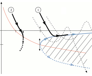
Phase space ‘detonation velocity versus radius’ ($y$–$x$) in the non-dimensional form $y\equiv b\,\dot{\unicode[STIX]{x1D6FC}}_{\unicode[STIX]{x1D70F}}=(b/\unicode[STIX]{x1D716})({\mathcal{D}}-{\mathcal{D}}_{o_{CJ}})/a_{u}$, $x\equiv 1/(2b\unicode[STIX]{x1D705})$. The equation of the CJ peninsula $\overline{y}_{_{CJ}}(x)$ is (4.12) and the quasi-steady trajectories $\overline{y}(x)$ are given in (7.1). The trajectories $\overline{y}_{1}(x)$ and $\overline{y}_{2}(x)$ represent respectively success of detonation initiation and failure.

(4.8a,b)$$\begin{eqnarray}\unicode[STIX]{x1D705}>0:\quad \overline{\dot{\unicode[STIX]{x1D6FC}}}_{\unicode[STIX]{x1D70F}_{CJ}}<0\,\,\Rightarrow \,\,\overline{{\mathcal{D}}}_{_{CJ}}(\unicode[STIX]{x1D705})<{\mathcal{D}}_{o_{CJ}},\quad \unicode[STIX]{x1D705}=0:\quad \overline{\dot{\unicode[STIX]{x1D6FC}}}_{\unicode[STIX]{x1D70F}_{CJ}}=0\,\,\Rightarrow \,\,\overline{{\mathcal{D}}}_{_{CJ}}={\mathcal{D}}_{o_{CJ}}.\end{eqnarray}$$

For a thermal sensitivity that is sufficiently small, the function $\unicode[STIX]{x1D705}(\overline{\dot{\unicode[STIX]{x1D6FC}}}_{\unicode[STIX]{x1D70F}_{CJ}})=-(\overline{\dot{\unicode[STIX]{x1D6FC}}}_{\unicode[STIX]{x1D70F}_{CJ}}/4)(2+\overline{\dot{\unicode[STIX]{x1D6FC}}}_{\unicode[STIX]{x1D70F}_{CJ}})\text{e}^{b\overline{\dot{\unicode[STIX]{x1D6FC}}}_{\unicode[STIX]{x1D70F}_{CJ}}}/(1+\overline{\dot{\unicode[STIX]{x1D6FC}}}_{\unicode[STIX]{x1D70F}_{CJ}})$ in (4.7) is decreasing monotonically from infinity to zero when $\overline{\dot{\unicode[STIX]{x1D6FC}}}_{\unicode[STIX]{x1D70F}_{CJ}}$ increases from $-1$ to $0$, $\text{d}\unicode[STIX]{x1D705}/\text{d}\overline{\dot{\unicode[STIX]{x1D6FC}}}_{\unicode[STIX]{x1D70F}_{CJ}}<0$ so that the detonation velocity decreases monotonically when the curvature increases from $0$ to $+\infty$ (radius decreases from $\infty$ to $0$). The situation is different for a thermal sensitivity that is sufficiently large; the function $\unicode[STIX]{x1D705}(\overline{\dot{\unicode[STIX]{x1D6FC}}}_{\unicode[STIX]{x1D70F}_{CJ}})$ presents two local extrema in the range $\overline{\dot{\unicode[STIX]{x1D6FC}}}_{\unicode[STIX]{x1D70F}_{CJ}}\in [-1,0]$ so that the curve $\overline{\dot{\unicode[STIX]{x1D6FC}}}_{\unicode[STIX]{x1D70F}_{CJ}}(\unicode[STIX]{x1D705})$ has an S-shaped form. This is already the case for $b=3.2$. For a large thermal sensitivity $b\gg 1$ the situation is the same as in He & Clavin (Reference He and Clavin1994), see figure 1 below. The graph ‘propagation velocity of the spherical CJ detonation versus the curvature’ $\overline{{\mathcal{D}}}_{_{CJ}}(\unicode[STIX]{x1D705})$ presents a turning point at a critical radius $r=r^{\ast }$ corresponding to a small curvature $\unicode[STIX]{x1D705}^{\ast }=O(1/b)$. The difference $({\mathcal{D}}_{o_{CJ}}-\overline{{\mathcal{D}}}_{_{CJ}})/(\unicode[STIX]{x1D716}{\mathcal{D}}_{o_{CJ}})>0$ is small, of order $1/b$, in the upper branch of solutions (the one going to ${\mathcal{D}}_{o_{CJ}}$ at large radius, see figure 1) while it is of order unity in the third branch of solutions (not represented in figure 1) which is non-physical because it corresponds to a too small Neumann temperature. In other words, there is no physical solution for $r<r^{\ast }$. Focusing our attention on radii of the same order of magnitude as the critical radius,

(4.9a,b)$$\begin{eqnarray}1/b\ll 1:\quad \unicode[STIX]{x1D705}=O(1/b),\quad |\overline{\dot{\unicode[STIX]{x1D6FC}}}_{\unicode[STIX]{x1D70F}_{CJ}}|=O(1/b)\quad \Rightarrow \quad \text{e}^{-b\,\overline{\dot{\unicode[STIX]{x1D6FC}}}_{\unicode[STIX]{x1D70F}_{CJ}}}=O(1),\end{eqnarray}$$

the terms smaller than $1/b$ can be neglected in (4.7),

(4.10)$$\begin{eqnarray}1/b\ll 1:\quad -\overline{\dot{\unicode[STIX]{x1D6FC}}}_{\unicode[STIX]{x1D70F}_{CJ}}=2\unicode[STIX]{x1D705}\text{e}^{-b\,\overline{\dot{\unicode[STIX]{x1D6FC}}}_{\unicode[STIX]{x1D70F}_{CJ}}}>0.\end{eqnarray}$$

In the limit $b\gg 1$ the quantities of order unity for the propagation velocity and the radius in the upper branch of detonations are respectively,

(4.11a,b)$$\begin{eqnarray}\overline{y}_{_{CJ}}\equiv b\,\overline{\dot{\unicode[STIX]{x1D6FC}}}_{\unicode[STIX]{x1D70F}_{CJ}}=\frac{b}{\unicode[STIX]{x1D716}}\left(\frac{\overline{{\mathcal{D}}}_{_{CJ}}-{\mathcal{D}}_{o_{CJ}}}{a_{u}}\right),\quad \frac{1}{x}\equiv 2\,b\,\unicode[STIX]{x1D705}=2\frac{b}{\unicode[STIX]{x1D716}}\left(\frac{l_{o_{CJ}}}{r_{f}}\right)>0,\end{eqnarray}$$

where $l_{o_{CJ}}=a_{u}t_{r}$ denotes the thickness of the planar CJ detonation, $t_{r}$ being the reaction time at the Neumann state (reference time) and, according to (3.15), $b/\unicode[STIX]{x1D716}=2(\unicode[STIX]{x1D6FE}-1){\mathcal{E}}/k_{B}T_{u}$. The propagation velocity of a quasi-steady spherical CJ wave $\overline{y}_{_{CJ}}(x)$ in term of its radius $x$ is, according to (4.10), the solution to

(4.12)$$\begin{eqnarray}\displaystyle & \displaystyle 1/b\ll 1:\quad -\overline{y}_{_{CJ}}\text{e}^{\overline{y}_{_{CJ}}}=1/x\quad \Leftrightarrow \quad \overline{y}_{_{CJ}}+\frac{1}{x}\text{e}^{-\overline{y}_{_{CJ}}}=0,\quad & \displaystyle\end{eqnarray}$$

(4.13)$$\begin{eqnarray}\displaystyle & \displaystyle \frac{\text{d}\overline{y}_{_{CJ}}}{\text{d}x}=\frac{\text{e}^{-\overline{y}_{_{CJ}}}}{x^{2}}\frac{1}{1+\overline{y}_{_{CJ}}}. & \displaystyle\end{eqnarray}$$

Because the terms of order $\unicode[STIX]{x1D716}$ have been neglected in (4.1), equations (4.10) and (4.12) are valid in the limit of small heat release ($\unicode[STIX]{x1D716}\ll 1$) for intermediate values of $1/b$,

(4.14)$$\begin{eqnarray}\unicode[STIX]{x1D716}\ll 1/b\ll 1.\end{eqnarray}$$

The solution (4.12), $\overline{y}_{_{CJ}}(x)$, is plotted in blue in figure 1, where the arrows indicate the direction of propagation ($\overline{y}_{_{CJ}}>-1:\text{d}\overline{y}_{_{CJ}}/\text{d}x>0$; $\overline{y}_{_{CJ}}<-1:\text{d}\overline{y}_{_{CJ}}/\text{d}x<0$). The critical value $r_{f}^{\ast }$ is larger than the detonation thickness of the planar CJ wave, $r_{f}^{\ast }\gg l_{o_{CJ}}$,

(4.15a-d)$$\begin{eqnarray}\overline{y}_{_{CJ}}^{\ast }=-1,\quad x^{\ast }=\text{e},\quad r_{f}^{\ast }/l_{o_{CJ}}=2\,\text{e}\,b/\unicode[STIX]{x1D716}\gg 1,\quad ({\mathcal{D}}_{o_{CJ}}-{\mathcal{D}}^{\ast })/a_{u}=\unicode[STIX]{x1D716}/b\ll 1,\end{eqnarray}$$

corresponding effectively to the orders of magnitude anticipated in (4.9),

(4.16a,b)$$\begin{eqnarray}b\gg 1:\quad \unicode[STIX]{x1D705}^{\ast }=(2\,\text{e})^{-1}/b,\quad \overline{\dot{\unicode[STIX]{x1D6FC}}}_{\unicode[STIX]{x1D70F}_{CJ}}^{\ast }=-1/b.\end{eqnarray}$$

Close to the critical radius, the CJ velocity $\overline{y}_{_{CJ}}$ varies as the square root of the radius $x$

(4.17)$$\begin{eqnarray}0<(x-\text{e})/\text{e}\ll 1:\quad \overline{y}_{_{CJ}}\approx -1+\sqrt{2}\sqrt{(x-\text{e})/\text{e}}.\end{eqnarray}$$

According to (4.12), the two branches of solutions $0>\overline{y}_{_{CJ+}}(x)>\overline{y}_{_{CJ-}}(x)$ for $x>x^{\ast }$ ($r_{f}>r_{f}^{\ast }$) merge at the critical radius $r_{f}=r_{f}^{\ast }$; $x=x^{\ast }$: $\overline{y}_{_{CJ+}}=\overline{y}_{_{CJ-}}=y^{\ast }=-1$. Both branches correspond to detonation velocities smaller than the velocity of the planar CJ wave, $\overline{y}_{_{CJ}\pm }<0$, ${\mathcal{D}}<{\mathcal{D}}_{o_{CJ}}$. According to (4.13), the upper (lower) branch of solutions $\overline{y}_{_{CJ+}}(x)>-1$, ($\overline{y}_{_{CJ-}}(x)<-1$,) is an increasing (decreasing) function of $x$, $\lim _{x\rightarrow \infty }\overline{y}_{_{CJ+}}=0$ ($\lim _{x\rightarrow \infty }\overline{y}_{_{CJ-}}=-\infty$), see figure 1. The solution $\overline{{\mathcal{D}}}_{_{CJ}}(r_{f})$ corresponding to $\overline{y}_{_{CJ+}}$ is an increasing function of the radius from ${\mathcal{D}}^{\ast }$ at $r_{f}=r_{f}^{\ast }$ up to the velocity of the planar CJ detonation for infinitely large radius, $\lim _{r_{f}/l_{o_{CJ}}\rightarrow \infty }\overline{{\mathcal{D}}}_{_{CJ}}={\mathcal{D}}_{o_{CJ}}$. This branch of solutions is shown in § 7 to play the role of an attractor for the quasi-steady trajectories when the initiation process is successful. The physical mechanism of the curvature-induced quenching is clearly identified from (4.7) to be the thermal sensitivity, responsible for the nonlinear variation of the detonation thickness with the propagation velocity through the Neumann temperature and the Rankine–Hugoniot conditions.

In the opposite limit of a large propagation Mach number $M\gg 1$ used in He & Clavin (Reference He and Clavin1994), the expression of the Rankine–Hugoniot condition

(4.18)$$\begin{eqnarray}\displaystyle (\unicode[STIX]{x1D6FE}-1)M^{2}\gg 1:\quad \frac{\unicode[STIX]{x1D6FF}T_{N}}{T_{N}}\approx 2\frac{\unicode[STIX]{x1D6FF}M}{M} & & \displaystyle\end{eqnarray}$$

differs quantitatively from (3.14). However, the same phenomenology is described in the limit of small heat release (3.1) which will helpful in the following to provide us with a qualitative description of the unsteady effects in the initiation process. The dynamics of a stable detonation on the upper branch of the CJ peninsula is effectively slow, except very close to the turning point. Unfortunately, according to (4.11), (4.13) and $\text{d}r_{f}/\text{d}t=\overline{{\mathcal{D}}}_{_{CJ}}$, the unsteady term is of the same order of magnitude as the curvature term, $1/b$,

(4.19)$$\begin{eqnarray}\frac{\text{d}\overline{y}_{_{CJ}}}{\text{d}\unicode[STIX]{x1D70F}}=\frac{1}{2\,b}\frac{\text{e}^{-\overline{y}_{_{CJ}}}}{x^{2}}\frac{1}{1+\overline{y}_{_{CJ}}}.\end{eqnarray}$$

4.3 Critical conditions for a smooth distribution of the reaction rate in the limit (4.14)

To leading order in the limit $b\gg 1$, the results (4.12)–(4.13) obtained with the square-wave model are still valid for a smooth distribution of the reaction rate provided the factor 2 in the expression (4.11) of $1/x$ is replaced by $\unicode[STIX]{x1D706}\in [1,\,2]$ where

(4.20a-c)$$\begin{eqnarray}b\gg 1:\quad 1/x=\unicode[STIX]{x1D706}\,b\,\unicode[STIX]{x1D705},\,\,\unicode[STIX]{x1D706}\equiv 1+\int _{-1}^{0}\unicode[STIX]{x1D707}_{o_{CJ}}(\unicode[STIX]{x1D709})\,\text{d}\unicode[STIX]{x1D709},\,\,x^{\ast }=\text{e}\,\,\Rightarrow \,\,r_{f}^{\ast }/l_{o_{CJ}}=\unicode[STIX]{x1D706}\,\text{e}\,b/\unicode[STIX]{x1D716},\end{eqnarray}$$

$\unicode[STIX]{x1D707}_{o_{CJ}}(\unicode[STIX]{x1D709})$ being the planar CJ solution obtained from (4.1) for $\unicode[STIX]{x1D705}=0$ and $\overline{\dot{\unicode[STIX]{x1D6FC}}}_{\unicode[STIX]{x1D70F}}=0$

(4.21a,b)$$\begin{eqnarray}\unicode[STIX]{x1D707}_{o_{CJ}}(\unicode[STIX]{x1D709})=\sqrt{\int _{-1}^{\unicode[STIX]{x1D709}}\unicode[STIX]{x1D714}_{o_{CJ}}(\unicode[STIX]{x1D709}^{\prime })\,\text{d}\unicode[STIX]{x1D709}^{\prime }},\quad \int _{-1}^{0}\unicode[STIX]{x1D714}_{o_{CJ}}(\unicode[STIX]{x1D709}^{\prime })\,\text{d}\unicode[STIX]{x1D709}^{\prime }=1,\,0<\unicode[STIX]{x1D707}_{o_{CJ}}(\unicode[STIX]{x1D709})<1,\,1<\unicode[STIX]{x1D706}<2.\end{eqnarray}$$

The proof is as follows. Consider a spherical CJ wave in the limit $1/b\ll 1$, $\overline{y}_{_{CJ}}\equiv b\overline{\dot{\unicode[STIX]{x1D6FC}}}_{\unicode[STIX]{x1D70F}_{CJ}}=O(1)$, $\unicode[STIX]{x1D705}=O(1/b)$, $\overline{\unicode[STIX]{x1D707}}_{b_{CJ}}=\overline{\dot{\unicode[STIX]{x1D6FC}}}_{\unicode[STIX]{x1D70F}_{CJ}}=O(1/b)$. Neglecting terms smaller than $1/b$ in (4.1), the function $\overline{\unicode[STIX]{x1D707}}_{_{CJ}}(\unicode[STIX]{x1D709})$ in the brackets on the right-hand side can be replaced by the steady solution for $\unicode[STIX]{x1D705}=0$ but with $b\overline{\dot{\unicode[STIX]{x1D6FC}}}_{\unicode[STIX]{x1D70F}_{CJ}}\neq 0$. This is the zeroth-order solution $\overline{\unicode[STIX]{x1D707}}_{o_{CJ}}$ of the curved CJ wave $\overline{\unicode[STIX]{x1D707}}_{_{CJ}}(\unicode[STIX]{x1D709})$ which can be expressed in terms of the velocity distribution of the planar CJ solution $\unicode[STIX]{x1D707}_{o_{CJ}}(\unicode[STIX]{x1D709})$ in the form $\overline{\unicode[STIX]{x1D707}}_{o_{CJ}}(\unicode[STIX]{x1D709})=\unicode[STIX]{x1D707}_{o_{CJ}}(\unicode[STIX]{x1D709}\text{e}^{\overline{y}_{_{CJ}}})$, as shown by (4.1), (4.2) and (4.4) in which the terms of order $1/b$ are neglected

(4.22a-c)$$\begin{eqnarray}\overline{\unicode[STIX]{x1D707}}_{o_{CJ}}\frac{\text{d}\overline{\unicode[STIX]{x1D707}}_{o_{CJ}}}{\text{d}\unicode[STIX]{x1D709}}=\frac{1}{2}\text{e}^{\overline{y}_{_{CJ}}}\unicode[STIX]{x1D714}_{o_{CJ}}(\unicode[STIX]{x1D709}\,\text{e}^{\overline{y}_{_{CJ}}}),\quad \unicode[STIX]{x1D709}=0:\quad \overline{\unicode[STIX]{x1D707}}_{o_{CJ}}=1,\quad \unicode[STIX]{x1D709}=-\text{e}^{-\overline{y}_{_{CJ}}}:\quad \overline{\unicode[STIX]{x1D707}}_{o_{CJ}}=0,\end{eqnarray}$$

(4.23a,b)$$\begin{eqnarray}\overline{\unicode[STIX]{x1D707}}_{o_{CJ}}^{2}(\unicode[STIX]{x1D709})=\int _{-\text{e}^{-\overline{y}_{_{CJ}}}}^{\unicode[STIX]{x1D709}}\text{e}^{\overline{y}_{_{CJ}}}\unicode[STIX]{x1D714}_{o_{CJ}}(\unicode[STIX]{x1D709}^{\prime }\,\text{e}^{\overline{y}_{_{CJ}}})\,\text{d}\unicode[STIX]{x1D709}^{\prime },\quad \overline{\unicode[STIX]{x1D707}}_{o_{CJ}}(\unicode[STIX]{x1D709})=\unicode[STIX]{x1D707}_{o_{CJ}}(\unicode[STIX]{x1D709}\text{e}^{\overline{y}_{_{CJ}}}),\end{eqnarray}$$

where $\unicode[STIX]{x1D707}_{o_{CJ}}(\unicode[STIX]{x1D709})$ is the planar solution (4.21). Equation (4.23) means that the leading order of the distribution $\overline{\unicode[STIX]{x1D707}}_{_{CJ}}(\unicode[STIX]{x1D709})$ in the limit $b\gg 1$ is obtained from the planar CJ solution by rescaling the length with the thickness of the spherical CJ detonation. At the leading order in the limit $b\gg 1$, integration of $\overline{\unicode[STIX]{x1D707}}_{_{CJ}}(\unicode[STIX]{x1D709})$ yields

(4.24)$$\begin{eqnarray}\displaystyle \int _{-\text{e}^{-\overline{y}_{_{CJ}}}}^{0}\overline{\unicode[STIX]{x1D707}}_{_{CJ}}\,\text{d}\unicode[STIX]{x1D709}\approx \text{e}^{-\overline{y}_{_{CJ}}}\int _{-1}^{0}\unicode[STIX]{x1D707}_{o_{CJ}}(z)\,\text{d}z=\text{e}^{-\overline{y}_{_{CJ}}}(\unicode[STIX]{x1D706}-1). & & \displaystyle\end{eqnarray}$$

Introducing (4.24) into (4.5) leads to (4.12) with the definition (4.20) of $x$, $x=1/(b\unicode[STIX]{x1D706}\unicode[STIX]{x1D705})$. The function $\unicode[STIX]{x1D707}_{o_{CJ}}(\unicode[STIX]{x1D709})>0$ varying monotonically from 0 at the exit of the reaction zone of the planar CJ detonation ($\unicode[STIX]{x1D709}_{ob_{CJ}}=-1$) to 1 at the Neumann state ($\unicode[STIX]{x1D709}=0$), $0<\int _{-1}^{0}\unicode[STIX]{x1D707}_{o_{CJ}}(\unicode[STIX]{x1D709}^{\prime })\,\text{d}\unicode[STIX]{x1D709}^{\prime }<1$, the parameter $\unicode[STIX]{x1D706}$ is in between 1 and 2, $1<\unicode[STIX]{x1D706}<2$. By comparison with (4.15), the critical radius for a smooth distribution in (4.20) is smaller than for the square-wave model by a factor $\unicode[STIX]{x1D706}/2<1$.

5.1 Curved CJ detonation in steady state. Sonic point

Using the notation (4.20), equation (4.1) takes the form

(5.1)$$\begin{eqnarray}\displaystyle 2\left[\overline{\unicode[STIX]{x1D707}}_{_{CJ}}(\unicode[STIX]{x1D709},\overline{y}_{_{CJ}})-\overline{y}_{_{CJ}}/b\right]\frac{\text{d}\overline{\unicode[STIX]{x1D707}}_{_{CJ}}}{\text{d}\unicode[STIX]{x1D709}}=\text{e}^{\overline{y}_{_{CJ}}}\unicode[STIX]{x1D714}_{o_{CJ}}(\unicode[STIX]{x1D709}\text{e}^{\overline{y}_{_{CJ}}})-\frac{1}{b}\left[1+\unicode[STIX]{x1D707}_{o_{CJ}}(\unicode[STIX]{x1D709}\text{e}^{\overline{y}_{_{CJ}}})\right]\frac{2}{\unicode[STIX]{x1D706}x}, & & \displaystyle\end{eqnarray}$$

where the $\overline{y}_{_{CJ}}$- dependence of the velocity distribution has been written explicitly in $\overline{\unicode[STIX]{x1D707}}_{_{CJ}}(\unicode[STIX]{x1D709},\overline{y}_{_{CJ}})$. Integration of (5.1) from the Neumann state (4.2) yields

(5.2)$$\begin{eqnarray}\displaystyle \left[\overline{\unicode[STIX]{x1D707}}_{_{CJ}}(\unicode[STIX]{x1D709},\overline{y}_{_{CJ}})-\frac{\overline{y}_{_{CJ}}}{b}\right]^{2} & = & \displaystyle \left(1+\frac{\overline{y}_{_{CJ}}}{b}\right)^{2}-\int _{\unicode[STIX]{x1D709}\text{e}^{\overline{y}_{_{CJ}}}}^{0}\unicode[STIX]{x1D714}_{o_{CJ}}(\unicode[STIX]{x1D709}^{\prime })\,\text{d}\unicode[STIX]{x1D709}^{\prime }\nonumber\\ \displaystyle & & \displaystyle +\,\left[-\unicode[STIX]{x1D709}\text{e}^{\overline{y}_{_{CJ}}}+\int _{\unicode[STIX]{x1D709}\text{e}^{\overline{y}_{_{CJ}}}}^{0}\unicode[STIX]{x1D707}_{o_{CJ}}(\unicode[STIX]{x1D709}^{\prime })\,\text{d}\unicode[STIX]{x1D709}^{\prime }\right]\frac{2}{b}\frac{\text{e}^{-\overline{y}_{_{CJ}}}}{\unicode[STIX]{x1D706}\,x},\end{eqnarray}$$

which takes the following form when using (3.16), (4.20) and (4.21), $\int _{-1}^{0}\unicode[STIX]{x1D714}_{o_{CJ}}(\unicode[STIX]{x1D709}^{\prime })\,\text{d}\unicode[STIX]{x1D709}^{\prime }$$=1$, $\unicode[STIX]{x1D706}\equiv 1+\int _{-1}^{0}\unicode[STIX]{x1D707}_{o_{CJ}}(\unicode[STIX]{x1D709}^{\prime })\,\text{d}\unicode[STIX]{x1D709}^{\prime }$ and $\unicode[STIX]{x1D707}_{o_{CJ}}(\unicode[STIX]{x1D709})=\int _{-1}^{\unicode[STIX]{x1D709}}\unicode[STIX]{x1D714}_{o_{CJ}}(\unicode[STIX]{x1D709}^{\prime })\,\text{d}\unicode[STIX]{x1D709}^{\prime }$,

(5.3)$$\begin{eqnarray}\displaystyle & & \displaystyle \left[\overline{\unicode[STIX]{x1D707}}_{_{CJ}}(\unicode[STIX]{x1D709},\overline{y}_{_{CJ}})-\frac{\overline{y}_{_{CJ}}}{b}\right]^{2}-\frac{\overline{y}_{_{CJ}}^{2}}{b^{2}}=\unicode[STIX]{x1D707}_{o_{CJ}}^{2}(\unicode[STIX]{x1D709}\text{e}^{\overline{y}_{_{CJ}}})\nonumber\\ \displaystyle & & \displaystyle \quad \quad +\frac{2}{b}\left\{\left[\overline{y}_{_{CJ}}+\frac{\text{e}^{-\overline{y}_{_{CJ}}}}{x}\right]-\frac{\text{e}^{-\overline{y}_{_{CJ}}}}{\unicode[STIX]{x1D706}\,x}\left[(\text{e}^{\overline{y}_{_{CJ}}}\unicode[STIX]{x1D709}+1)+\int _{-1}^{\unicode[STIX]{x1D709}\text{e}^{\overline{y}_{_{CJ}}}}\unicode[STIX]{x1D707}_{o_{CJ}}(\unicode[STIX]{x1D709}^{\prime })\,\text{d}\unicode[STIX]{x1D709}^{\prime }\right]\right\}.\quad\end{eqnarray}$$

In the limit (4.14), equation (5.3) shows that the difference $\overline{\unicode[STIX]{x1D707}}_{_{CJ}}(\unicode[STIX]{x1D709},\overline{y}_{_{CJ}})-\unicode[STIX]{x1D707}_{o_{CJ}}(\unicode[STIX]{x1D709}\text{e}^{\overline{y}_{_{CJ}}})$ is smaller than unity. Neglecting terms of order $1/b^{2}$, equations (4.12) with (4.20) are recovered from (5.3) if the sonic condition $\left(\overline{\unicode[STIX]{x1D707}}_{_{CJ}}-\overline{y}_{_{CJ}}/b\right)=0$ is assumed to hold at the end of the heat release, $\overline{\unicode[STIX]{x1D709}}_{_{CJ}}\text{e}^{\overline{y}_{_{CJ}}}=-1$ where $\unicode[STIX]{x1D709}=-1$ is the reduced position of the exit of the reaction zone in the planar CJ wave, $\unicode[STIX]{x1D714}_{o_{CJ}}(-1)=0$; $\unicode[STIX]{x1D709}\leqslant -\text{e}^{-\overline{y}_{_{CJ}}}:\unicode[STIX]{x1D714}_{o_{CJ}}(\unicode[STIX]{x1D709}\text{e}^{\overline{y}_{_{CJ}}})=0$ and $\unicode[STIX]{x1D707}_{o_{CJ}}(\unicode[STIX]{x1D709}\text{e}^{\overline{y}_{_{CJ}}})=0$, see (4.21). In fact, the sonic condition holds inside the detonation thickness just before the end of the exothermal reaction. Denoting by $\overline{\unicode[STIX]{x1D709}}_{s_{CJ}}$ its position,

(5.4)$$\begin{eqnarray}\displaystyle \unicode[STIX]{x1D709}=\overline{\unicode[STIX]{x1D709}}_{s_{CJ}}:\quad \left(\overline{\unicode[STIX]{x1D707}}_{_{CJ}}-\overline{y}_{_{CJ}}/b\right)=0, & & \displaystyle\end{eqnarray}$$

a first relation linking $\overline{y}_{_{CJ}}$ and $\overline{\unicode[STIX]{x1D709}}_{s_{CJ}}$ is given by (5.2)–(5.3)

(5.5)$$\begin{eqnarray}\displaystyle \unicode[STIX]{x1D707}_{o_{CJ}}^{2}(\overline{\unicode[STIX]{x1D709}}_{s_{CJ}}\text{e}^{\overline{y}_{_{CJ}}})+\frac{2}{b}\left[\overline{y}_{_{CJ}}+\frac{\text{e}^{-\overline{y}_{_{CJ}}}}{\unicode[STIX]{x1D706}\,x}\int _{\overline{\unicode[STIX]{x1D709}}_{s_{CJ}}\text{e}^{\overline{y}_{_{CJ}}}}^{0}[1+\unicode[STIX]{x1D707}_{o_{CJ}}(\unicode[STIX]{x1D709}^{\prime })]\,\text{d}\unicode[STIX]{x1D709}^{\prime }\right]+\frac{\overline{y}_{_{CJ}}^{2}}{b^{2}}=0.\quad & & \displaystyle\end{eqnarray}$$

The second relation necessary to determine $\overline{y}_{_{CJ}}$ and $\overline{\unicode[STIX]{x1D709}}_{s_{CJ}}$ is obtained from (5.1) if the derivative $\text{d}\overline{\unicode[STIX]{x1D707}}_{_{CJ}}(\unicode[STIX]{x1D709},\overline{y}_{_{CJ}})/\text{d}\unicode[STIX]{x1D709}|_{\unicode[STIX]{x1D709}=-1}$ is bounded

(5.6)$$\begin{eqnarray}\displaystyle \text{e}^{\overline{y}_{_{CJ}}}\unicode[STIX]{x1D714}_{o_{CJ}}(\overline{\unicode[STIX]{x1D709}}_{s_{CJ}}\text{e}^{\overline{y}_{_{CJ}}})=\frac{1}{b}\left[1+\unicode[STIX]{x1D707}_{o_{CJ}}(\overline{\unicode[STIX]{x1D709}}_{s_{CJ}}\text{e}^{\overline{y}_{_{CJ}}})\right]\frac{2}{\unicode[STIX]{x1D706}x}\,\,\Rightarrow \,\,\unicode[STIX]{x1D714}_{o_{CJ}}(\overline{\unicode[STIX]{x1D709}}_{s_{CJ}}\text{e}^{\overline{y}_{_{CJ}}})=O(1/b) & & \displaystyle\end{eqnarray}$$

showing that the reaction is not completed at the sonic point $\unicode[STIX]{x1D714}_{o_{CJ}}(\overline{\unicode[STIX]{x1D709}}_{s_{CJ}}\text{e}^{\overline{y}_{_{CJ}}})>0$, $\overline{\unicode[STIX]{x1D709}}_{s_{CJ}}>-\text{e}^{-\overline{y}_{_{CJ}}}$, the reaction rate being, however, small, of order $1/b$. Subtracting (5.5) from (5.3) yields

(5.7)$$\begin{eqnarray}\displaystyle & & \displaystyle \unicode[STIX]{x1D709}\geqslant \overline{\unicode[STIX]{x1D709}}_{s_{CJ}}>-\text{e}^{-\overline{y}_{_{CJ}}}:\quad \left[\overline{\unicode[STIX]{x1D707}}_{_{CJ}}(\unicode[STIX]{x1D709},\overline{y}_{_{CJ}})-\frac{\overline{y}_{_{CJ}}}{b}\right]^{2}\nonumber\\ \displaystyle & & \displaystyle \quad =\int _{\overline{\unicode[STIX]{x1D709}}_{s_{CJ}}\text{e}^{\overline{y}_{_{CJ}}}}^{\unicode[STIX]{x1D709}\text{e}^{\overline{y}_{_{CJ}}}}\unicode[STIX]{x1D714}_{o_{CJ}}(\unicode[STIX]{x1D709}^{\prime })\,\text{d}\unicode[STIX]{x1D709}^{\prime }-\frac{1}{b}\left[(\unicode[STIX]{x1D709}-\overline{\unicode[STIX]{x1D709}}_{s_{CJ}})\text{e}^{\overline{y}_{_{CJ}}}+\int _{\overline{\unicode[STIX]{x1D709}}_{s_{CJ}}\text{e}^{\overline{y}_{_{CJ}}}}^{\unicode[STIX]{x1D709}\text{e}^{\overline{y}_{_{CJ}}}}\unicode[STIX]{x1D707}_{o_{CJ}}(\unicode[STIX]{x1D709}^{\prime })\,\text{d}\unicode[STIX]{x1D709}^{\prime }\right]\frac{2\text{e}^{-\overline{y}_{_{CJ}}}}{\unicode[STIX]{x1D706}x},\end{eqnarray}$$

so that the right-hand side should be positive

(5.8)$$\begin{eqnarray}\displaystyle \int _{\overline{\unicode[STIX]{x1D709}}_{s_{CJ}}\text{e}^{\overline{y}_{_{CJ}}}}^{\unicode[STIX]{x1D709}\text{e}^{\overline{y}_{_{CJ}}}}\unicode[STIX]{x1D714}_{o_{CJ}}(\unicode[STIX]{x1D709}^{\prime })\,\text{d}\unicode[STIX]{x1D709}^{\prime }\geqslant \frac{1}{b}\left[(\unicode[STIX]{x1D709}-\overline{\unicode[STIX]{x1D709}}_{s_{CJ}})\text{e}^{\overline{y}_{_{CJ}}}+\int _{\overline{\unicode[STIX]{x1D709}}_{s_{CJ}}\text{e}^{\overline{y}_{_{CJ}}}}^{\unicode[STIX]{x1D709}\text{e}^{\overline{y}_{_{CJ}}}}\unicode[STIX]{x1D707}_{o_{CJ}}(\unicode[STIX]{x1D709}^{\prime })\,\text{d}\unicode[STIX]{x1D709}^{\prime }\right]\frac{2\text{e}^{-\overline{y}_{_{CJ}}}}{\unicode[STIX]{x1D706}x}.\quad & & \displaystyle\end{eqnarray}$$

The inequality is automatically satisfied in the range $0<(\unicode[STIX]{x1D709}-\overline{\unicode[STIX]{x1D709}}_{s_{CJ}})=O(1)$ for $b\gg 1$ and $|\overline{y}_{_{CJ}}|=O(1)$ because the functions $\unicode[STIX]{x1D714}_{o_{CJ}}(\unicode[STIX]{x1D709})$ and $\unicode[STIX]{x1D707}_{o_{CJ}}(\unicode[STIX]{x1D709})$ are of order unity and positive for $\unicode[STIX]{x1D709}>-1$. Both sides of (5.8) are increasing functions of $\unicode[STIX]{x1D709}$ from 0 at $\unicode[STIX]{x1D709}=\overline{\unicode[STIX]{x1D709}}_{s_{CJ}}$. The case $0<(\unicode[STIX]{x1D709}-\overline{\unicode[STIX]{x1D709}}_{s_{CJ}})\ll 1$ is easily investigated within the model (3.17) which will be used from now on. According to (3.17), the distribution of the reaction rate in the planar CJ wave is linear close to $\unicode[STIX]{x1D709}=-1$, $0<\unicode[STIX]{x1D709}+1\ll 1:\,\unicode[STIX]{x1D714}_{o_{CJ}}\approx h_{\unicode[STIX]{x1D714}}(\unicode[STIX]{x1D709}+1)$, $h_{\unicode[STIX]{x1D714}}>0$ and, according to (4.21), the slope of the velocity profile in the plane CJ wave is also positive and of order unity at the end of the reaction zone

(5.9)$$\begin{eqnarray}\unicode[STIX]{x1D709}\leqslant -1:\quad \unicode[STIX]{x1D707}_{o_{CJ}}=0\quad \text{but }\text{d}\unicode[STIX]{x1D707}_{o_{CJ}}/\text{d}\unicode[STIX]{x1D709}|_{\unicode[STIX]{x1D709}+1=0^{+}}=h_{\unicode[STIX]{x1D707}}>0,\end{eqnarray}$$

(5.10a,b)$$\begin{eqnarray}0<(\unicode[STIX]{x1D709}+1)\ll 1:\quad \unicode[STIX]{x1D707}_{o_{CJ}}(\unicode[STIX]{x1D709})\approx h_{\unicode[STIX]{x1D707}}(\unicode[STIX]{x1D709}+1),\quad h_{\unicode[STIX]{x1D707}}>0,\,h_{\unicode[STIX]{x1D707}}\equiv \sqrt{h_{\unicode[STIX]{x1D714}}/2}=O(1).\end{eqnarray}$$

Then, according to (5.6), $0<(\overline{\unicode[STIX]{x1D709}}_{s_{CJ}}+\text{e}^{-\overline{y}_{_{CJ}}})=O(1/b)$, the sonic condition can be safely applied at the exit of the reaction zone $\unicode[STIX]{x1D709}=-\text{e}^{-\overline{y}_{_{CJ}}}$. The first term of a Taylor expansion around $\unicode[STIX]{x1D709}=\overline{\unicode[STIX]{x1D709}}_{s_{CJ}}$ is the same on both sides of (5.8), and the second-order term satisfies the inequality (5.8) in the limit $b\gg 1$ when the second derivative $\text{d}^{2}\unicode[STIX]{x1D714}_{o_{CJ}}/\text{d}\unicode[STIX]{x1D709}^{2}|_{\unicode[STIX]{x1D709}+1\,=\,0^{+}}$ is of order unity (smaller than $b$). A Taylor expansion of (5.3) around the sonic point using (5.5)–(5.6) then yields

(5.11)$$\begin{eqnarray}\displaystyle 0\leqslant (\unicode[STIX]{x1D709}-\overline{\unicode[STIX]{x1D709}}_{s_{CJ}})\ll 1 & : & \displaystyle \quad \overline{\unicode[STIX]{x1D707}}_{_{CJ}}(\unicode[STIX]{x1D709},\overline{y}_{_{CJ}})-\frac{\overline{y}_{_{CJ}}}{b}\approx h_{\unicode[STIX]{x1D707}}\,\text{e}^{\overline{y}_{_{CJ}}}(\unicode[STIX]{x1D709}-\overline{\unicode[STIX]{x1D709}}_{s_{CJ}})\left[1+O\left(1/b\right)\right]\end{eqnarray}$$

(5.12)$$\begin{eqnarray}\displaystyle \unicode[STIX]{x1D709}<\overline{\unicode[STIX]{x1D709}}_{s_{CJ}} & : & \displaystyle \quad \overline{\unicode[STIX]{x1D707}}_{_{CJ}}(\unicode[STIX]{x1D709},\overline{y}_{_{CJ}})-\overline{y}_{_{CJ}}/b=0,\end{eqnarray}$$

and, more generally, one has

(5.13)$$\begin{eqnarray}\displaystyle x\geqslant \text{e}:\quad \overline{\unicode[STIX]{x1D707}}_{_{CJ}}(\unicode[STIX]{x1D709},\overline{y}_{_{CJ}}(x))=\unicode[STIX]{x1D707}_{o_{CJ}}(\unicode[STIX]{x1D709}\text{e}^{\overline{y}_{_{CJ}}(x)})\left[1+O\left(1/b\right)\right], & & \displaystyle\end{eqnarray}$$

valid everywhere inside the inner structure of the detonations on the upper branch of the CJ peninsula, even near the turning point $x=\text{e}$ where, to leading order, $\overline{y}_{_{CJ}}\approx -1$. The correction to (4.12)–(4.13) is then shown to be negligible

(5.14a,b)$$\begin{eqnarray}\displaystyle \overline{y}_{_{CJ}}+\frac{1}{x}\text{e}^{-\overline{y}_{_{CJ}}}=O(\overline{y}_{_{CJ}}^{2}/b),\quad \frac{\text{d}\overline{y}_{_{CJ}}}{\text{d}x}=\frac{\text{e}^{-\overline{y}_{_{CJ}}}}{x^{2}}\frac{1}{1+\overline{y}_{_{CJ}}\left[\,1+O(1/b)\,\right]}. & & \displaystyle\end{eqnarray}$$

5.2 Weakly overdriven regimes of spherical detonation

Consider now spherical detonations in a weakly overdriven regime. For a small curvature (4.9), to leading order in the limit (4.14), the term $\unicode[STIX]{x1D707}$ on the right-hand of (3.10) can be replaced by $\unicode[STIX]{x1D707}_{o_{CJ}}(\unicode[STIX]{x1D709}\text{e}^{b\overline{\dot{\unicode[STIX]{x1D6FC}}}_{\unicode[STIX]{x1D70F}}})$. Denoting the steady-state approximation by an overbar, the equation for $\overline{\unicode[STIX]{x1D707}}(\unicode[STIX]{x1D709})$ when the unsteady term is neglected in (3.10) reads

(5.15a,b)$$\begin{eqnarray}[\overline{\unicode[STIX]{x1D707}}(\unicode[STIX]{x1D709})-\overline{\dot{\unicode[STIX]{x1D6FC}}}_{\unicode[STIX]{x1D70F}}]\frac{\text{d}\overline{\unicode[STIX]{x1D707}}}{\text{d}\unicode[STIX]{x1D709}}=\frac{1}{2}\text{e}^{b\overline{\dot{\unicode[STIX]{x1D6FC}}}_{\unicode[STIX]{x1D70F}}}\unicode[STIX]{x1D714}_{o_{CJ}}(\unicode[STIX]{x1D709}\,\text{e}^{b\overline{\dot{\unicode[STIX]{x1D6FC}}}_{\unicode[STIX]{x1D70F}}})-[1+\unicode[STIX]{x1D707}_{o_{CJ}}(\unicode[STIX]{x1D709}\text{e}^{b\overline{\dot{\unicode[STIX]{x1D6FC}}}_{\unicode[STIX]{x1D70F}}})]\unicode[STIX]{x1D705},\quad \unicode[STIX]{x1D709}=0:\quad \overline{\unicode[STIX]{x1D707}}=1+2\overline{\dot{\unicode[STIX]{x1D6FC}}}_{\unicode[STIX]{x1D70F}}\end{eqnarray}$$

and the boundary condition at the exit of the inner structure, $\unicode[STIX]{x1D709}=\unicode[STIX]{x1D709}_{b}$, of a slightly overdriven detonation takes the form

(5.16a,b)$$\begin{eqnarray}\unicode[STIX]{x1D709}=\unicode[STIX]{x1D709}_{b}:\quad \overline{\unicode[STIX]{x1D707}}\approx \unicode[STIX]{x1D707}_{b},\quad 0<(\unicode[STIX]{x1D707}_{b}-\overline{\dot{\unicode[STIX]{x1D6FC}}}_{\unicode[STIX]{x1D70F}})\ll 1.\end{eqnarray}$$

If the boundary condition $\overline{\unicode[STIX]{x1D707}}=\unicode[STIX]{x1D707}_{b}$ is taken at the end of the reaction $\unicode[STIX]{x1D709}=-\text{e}^{-b\overline{\dot{\unicode[STIX]{x1D6FC}}}_{\unicode[STIX]{x1D70F}}}$, equation (5.15) would lead to a negative slope at the end of the inner structure, $(\unicode[STIX]{x1D707}_{b}-\overline{\dot{\unicode[STIX]{x1D6FC}}}_{\unicode[STIX]{x1D70F}})\,\text{d}\overline{\unicode[STIX]{x1D707}}/\text{d}\unicode[STIX]{x1D709}\approx -\unicode[STIX]{x1D705}<0$. This is not satisfactory for the problem of direct initiation since the flow in the rarefaction wave is an increasing function of the radius and the reaction is exothermic. In fact the unsteady term cannot be neglected in the matching region between the inner structure and the inert rarefaction flow (external flow). In this intermediate zone, the flow is quasi-uniform at the scale of the thickness of the inner structure and all the terms of (3.10) are small, of the order of magnitude of the reduced curvature $1/\unicode[STIX]{x1D705}=O(1/b)$ at most, in particular, the reaction rate,

(5.17)$$\begin{eqnarray}\displaystyle \text{e}^{b\dot{\unicode[STIX]{x1D6FC}}_{\unicode[STIX]{x1D70F}}}\unicode[STIX]{x1D714}_{o_{CJ}}(\unicode[STIX]{x1D709}_{b}\,\text{e}^{b\dot{\unicode[STIX]{x1D6FC}}_{\unicode[STIX]{x1D70F}}})=O(1/b), & & \displaystyle\end{eqnarray}$$

the term involving the flow gradient is even smaller

(5.18)$$\begin{eqnarray}\displaystyle [\unicode[STIX]{x1D707}-\dot{\unicode[STIX]{x1D6FC}}_{\unicode[STIX]{x1D70F}}]\,\text{d}\unicode[STIX]{x1D707}/\text{d}\unicode[STIX]{x1D709}=o(1/b). & & \displaystyle\end{eqnarray}$$

In that respect, the situation is similar to the CJ case, the place where the external condition (5.16) $\overline{\unicode[STIX]{x1D707}}=\unicode[STIX]{x1D707}_{b}$ is applied inside the inner structure is fairly close to the end of the reaction

(5.19)$$\begin{eqnarray}\displaystyle b\gg 1:\quad \unicode[STIX]{x1D709}_{b}=-\text{e}^{-b\dot{\unicode[STIX]{x1D6FC}}_{\unicode[STIX]{x1D70F}}}[1+O(1/b)]. & & \displaystyle\end{eqnarray}$$

and the difference from $-\text{e}^{-b\dot{\unicode[STIX]{x1D6FC}}_{\unicode[STIX]{x1D70F}}}$ will not influence the leading order of the propagation velocity and the calculation for a given flow velocity of burnt gas $\unicode[STIX]{x1D707}_{b}$ proceeds as in § 5.1. Focusing our attention on propagation velocities and radii close to their critical values, ${\mathcal{D}}^{\ast }$ and $r_{f}^{\ast }$ introduced in §§ 4.2–4.3, it is convenient to introduce the dimensionless variables $y$ and $x$ of order unity, similar to (4.11),

(5.20a,b)$$\begin{eqnarray}y\equiv b\dot{\unicode[STIX]{x1D6FC}}_{\unicode[STIX]{x1D70F}}=\frac{b}{\unicode[STIX]{x1D716}}\left(\frac{{\mathcal{D}}-{\mathcal{D}}_{o_{CJ}}}{a_{u}}\right)=O(1),\quad \frac{1}{x}\equiv \unicode[STIX]{x1D706}b\unicode[STIX]{x1D705}=O(1),\end{eqnarray}$$

the parameters $\unicode[STIX]{x1D716}\ll 1$, $b\gg 1$ and $\unicode[STIX]{x1D706}\in [1,2]$ being defined in (3.1), (3.15) and (4.20) respectively. Integration of (5.15) from the Neumann state at $\unicode[STIX]{x1D709}=0$ leads to an expression similar to (5.3)

(5.21)$$\begin{eqnarray}\displaystyle \!\!\left[\overline{\unicode[STIX]{x1D707}}(\unicode[STIX]{x1D709})-\frac{\overline{y}}{b}\right]^{2} & = & \displaystyle \frac{\overline{y}^{2}}{b^{2}}+\unicode[STIX]{x1D707}_{o_{CJ}}^{2}(\unicode[STIX]{x1D709}\text{e}^{\overline{y}})\nonumber\\ \displaystyle \!\! & & \displaystyle +\,\frac{2}{b}\left\{\!\left[\overline{y}+\frac{\text{e}^{-\overline{y}}}{x}\right]-\frac{\text{e}^{-\overline{y}}}{\unicode[STIX]{x1D706}\,x}\left[(\text{e}^{\overline{y}}\unicode[STIX]{x1D709}+1)+\int _{-1}^{\unicode[STIX]{x1D709}\text{e}^{\overline{y}}}\unicode[STIX]{x1D707}_{o_{CJ}}(\unicode[STIX]{x1D709}^{\prime })\,\text{d}\unicode[STIX]{x1D709}^{\prime }\right]\!\right\}\!.\end{eqnarray}$$

The boundary condition in the burnt gas (5.16) using (5.19) and $\unicode[STIX]{x1D707}_{o_{CJ}}(\unicode[STIX]{x1D709}_{b}\text{e}^{\overline{y}})=O(1/b)$, leads to the relation between $\overline{y}$ and $\unicode[STIX]{x1D707}_{b}$

(5.22)$$\begin{eqnarray}\displaystyle & \displaystyle b\unicode[STIX]{x1D707}_{b}^{2}/2-\overline{y}\unicode[STIX]{x1D707}_{b}=\overline{y}+\text{e}^{-\overline{y}}/x+O(1/b), & \displaystyle \nonumber\\ \displaystyle & \displaystyle \unicode[STIX]{x1D707}_{b}=O(1/\sqrt{b}):\quad b\unicode[STIX]{x1D707}_{b}^{2}/2=\overline{y}+\text{e}^{-\overline{y}}/x+O(1/\sqrt{b}), & \displaystyle\end{eqnarray}$$

where the last term on the right-hand side of (5.21) gives a negligible contribution, of order $1/b$. The ordering $\unicode[STIX]{x1D707}_{b}(\unicode[STIX]{x1D70F})=O(1/\sqrt{b})$ corresponds to a propagation velocity and a radius of the same order of magnitude as at the turning point, $\overline{y}=O(1)$ and $x=O(1)$. For slightly overdriven detonations in a planar geometry $\unicode[STIX]{x1D705}=0$, equations (5.21)–(5.22) reduce to (C 5)–(C 8) in appendix C and the classical square root relation is recovered between the flow velocity in the burnt gas (overdrive factor) and the departure of the detonation velocity from its CJ value, $\unicode[STIX]{x1D705}=0,\,\,0<\overline{\dot{\unicode[STIX]{x1D6FC}}}_{\unicode[STIX]{x1D70F}}\ll 1\,\,\Rightarrow \,\,\unicode[STIX]{x1D707}_{b}\approx \sqrt{2\overline{\dot{\unicode[STIX]{x1D6FC}}}_{\unicode[STIX]{x1D70F}}}$. According to (5.21), the $\unicode[STIX]{x1D709}$-variation of $\overline{\unicode[STIX]{x1D707}}(\unicode[STIX]{x1D709})$ is through the grouping $\unicode[STIX]{x1D709}\text{e}^{\overline{y}}$ like in $\unicode[STIX]{x1D707}_{o_{CJ}}(\unicode[STIX]{x1D709}\text{e}^{\overline{y}})$. The difference $\overline{\unicode[STIX]{x1D707}}(\unicode[STIX]{x1D709})-\unicode[STIX]{x1D707}_{o_{CJ}}(\unicode[STIX]{x1D709}\text{e}^{b\overline{\dot{\unicode[STIX]{x1D6FC}}}_{\unicode[STIX]{x1D70F}}})$ is of order $1/\sqrt{b}$ near the end of the reaction where $\unicode[STIX]{x1D707}_{o_{CJ}}(\unicode[STIX]{x1D709}\text{e}^{\overline{y}})$ is of order $1/\sqrt{b}$ while the difference is smaller, of order $1/b$, elsewhere inside the inner structure of the detonation. The quasi-steady trajectories (5.22) are analysed in § 7.1.

6.1 Flow of burnt gas near the detonation. Closure relation

In the analysis of Liñan et al. (Reference Liñan, Kurdyumov and Sanchez2012) (discontinuous model and $M\gg 1$), near the CJ regime, the quasi-transonic flow (relative to the detonation front) is described by a Burgers-like equation. The same equation is derived in the limit (3.1), $0<M-1\ll 1$ from (3.10) for the flow of burnt gas close to the end of the reaction zone

(6.1)$$\begin{eqnarray}\unicode[STIX]{x1D709}\leqslant \unicode[STIX]{x1D709}_{b},|\unicode[STIX]{x1D709}|=O(1):\quad \unicode[STIX]{x2202}\unicode[STIX]{x1D707}/\unicode[STIX]{x2202}\unicode[STIX]{x1D70F}+(\unicode[STIX]{x1D707}-\dot{\unicode[STIX]{x1D6FC}}_{\unicode[STIX]{x1D70F}})\unicode[STIX]{x2202}\unicode[STIX]{x1D707}/\unicode[STIX]{x2202}\unicode[STIX]{x1D709}=-\unicode[STIX]{x1D705}(\unicode[STIX]{x1D70F})\left[1+\unicode[STIX]{x1D707}\right],\end{eqnarray}$$

leading to the Burgers-like equation obtained by Liñan et al. (Reference Liñan, Kurdyumov and Sanchez2012)

(6.2)$$\begin{eqnarray}\dot{\unicode[STIX]{x1D6FC}}_{\unicode[STIX]{x1D70F}}<\unicode[STIX]{x1D707}<1:\quad \unicode[STIX]{x2202}\unicode[STIX]{x1D707}/\unicode[STIX]{x2202}\unicode[STIX]{x1D70F}+\unicode[STIX]{x1D707}\unicode[STIX]{x2202}\unicode[STIX]{x1D707}/\unicode[STIX]{x2202}\unicode[STIX]{x1D709}=-\unicode[STIX]{x1D705}.\end{eqnarray}$$

The curvature on the right-hand is quasi-constant when the radius gets close to the CJ condition. Going back to the dimensional form by using (3.2), (3.4), (3.7) and (3.9), equation (6.1) takes the more explicit form

(6.3)$$\begin{eqnarray}\displaystyle u(,t),\quad =r-r_{f}(t):\quad \frac{\unicode[STIX]{x2202}u}{\unicode[STIX]{x2202}t}+[a-({\mathcal{D}}-u)]\frac{\unicode[STIX]{x2202}u}{\unicode[STIX]{x2202}}=-\frac{a}{r}u, & & \displaystyle\end{eqnarray}$$

describing the propagation of the upstream-running mode in the rarefaction flow near the detonation where this flow is quasi-transonic, $a\gg a-({\mathcal{D}}-u)\geqslant 0$. In the laboratory frame, the flow behind an expending detonation ($\text{d}r_{f}/\text{d}t>0$, $\unicode[STIX]{x1D709}\leqslant \unicode[STIX]{x1D709}_{b}<0$) decreases when the distance from the detonation front increases; the flow is an increasing function of the radius, $\unicode[STIX]{x2202}u/\unicode[STIX]{x2202}r>0$. The burnt-gas flow of the rarefaction wave varies in space on a length scale $l_{ext}\equiv [(1/u)\unicode[STIX]{x2202}u/\unicode[STIX]{x2202}r]^{-1}$ typically of the order of magnitude of the radius of the lead shock $r_{f}$. When the radius is larger than the detonation thickness, $r_{f}\gg l$, the length scale of the external flow is larger than the detonation thickness $l_{ext}\gg l$. According to the quasi-transonic flow of burnt gas when approaching the CJ regime, $0\leqslant a-({\mathcal{D}}-u)\ll a$, the second term on the left-hand side of (6.1) and (6.3) (the one involving the derivative with respect to space) is smaller than the right-hand side and can be neglected. Therefore, near the end of the reaction zone, the instantaneous flow $u_{b}(t)$ or $\unicode[STIX]{x1D707}_{b}(\unicode[STIX]{x1D70F})$ is simply a function of the flow curvature

(6.4a-c)$$\begin{eqnarray}\frac{\text{d}\unicode[STIX]{x1D707}_{b}}{\text{d}\unicode[STIX]{x1D70F}}=-\unicode[STIX]{x1D705}(\unicode[STIX]{x1D70F})[1+\unicode[STIX]{x1D707}_{b}],\quad \frac{1}{u_{b}}\frac{\text{d}u_{b}}{\text{d}t}=-\frac{a}{r_{f}},\quad \unicode[STIX]{x1D707}_{b}(\unicode[STIX]{x1D70F})=[1+\unicode[STIX]{x1D707}_{bi}]\text{e}^{-\int _{0}^{\unicode[STIX]{x1D70F}}\unicode[STIX]{x1D705}(\unicode[STIX]{x1D70F}^{\prime })\,\text{d}\unicode[STIX]{x1D70F}^{\prime }}-1,\end{eqnarray}$$

where the subscript $i$ denotes the initial condition at $\unicode[STIX]{x1D70F}=0$. Introducing the reduced radius of the shock front (4.20), $x=1/(\unicode[STIX]{x1D706}\,b\,\unicode[STIX]{x1D705})$, and the definition (3.3) of $\dot{\unicode[STIX]{x1D6FC}}_{\unicode[STIX]{x1D70F}}$, the relations ${\mathcal{D}}\equiv \text{d}r_{f}/\text{d}t$, $\text{d}/\text{d}\unicode[STIX]{x1D70F}=(t_{r}/\unicode[STIX]{x1D716})\,\text{d}/\text{d}t$ and $l_{o_{CJ}}\equiv a_{u}t_{r}$, lead to

(6.5a-c)$$\begin{eqnarray}\frac{\text{d}x}{\text{d}\unicode[STIX]{x1D70F}}=\frac{1}{\unicode[STIX]{x1D706}b}\left[1+\unicode[STIX]{x1D716}(1+\dot{\unicode[STIX]{x1D6FC}}_{\unicode[STIX]{x1D70F}})\right]\approx \frac{1}{\unicode[STIX]{x1D706}b},\quad x(\unicode[STIX]{x1D70F})-x_{i}\approx \frac{\unicode[STIX]{x1D70F}}{b\unicode[STIX]{x1D706}},\quad \unicode[STIX]{x1D707}_{b}(\unicode[STIX]{x1D70F})\approx \unicode[STIX]{x1D707}_{bi}-\ln (x/x_{i}),\end{eqnarray}$$

where the last relation is obtained from the first relation in (6.4) for $\unicode[STIX]{x1D707}_{b}\ll 1$.

According to Liñan et al. (Reference Liñan, Kurdyumov and Sanchez2012), the scale separation insuring the validity of (6.4)–(6.5) breaks down abruptly as soon as the CJ regime is reached. Moreover, this occurs at a finite radius. Therefore the transition to the Chapman–Jouguet regime is abrupt, producing quasi-instantaneously a jump of flow gradient (not of the flow velocity) inside the rarefaction wave. The key point is that the velocity ${\mathcal{D}}(\unicode[STIX]{x1D70F})$ of an overdriven detonation whose inner structure is in steady state cannot decrease below the CJ velocity ${\mathcal{D}}_{o_{CJ}}$ so that the strong deceleration of the detonation ($\text{d}{\mathcal{D}}/\text{d}\unicode[STIX]{x1D70F}<0$) which is induced by the rarefaction wave is stopped suddenly ($\text{d}{\mathcal{D}}/\text{d}\unicode[STIX]{x1D70F}\approx 0$) when ${\mathcal{D}}(t)$ reaches ${\mathcal{D}}_{o_{CJ}}$. Then, the velocity gradient of the external flow at the detonation front jumps to infinity and remains infinite subsequently. Just after the transition, the unsteady term $\unicode[STIX]{x2202}\unicode[STIX]{x1D707}/\unicode[STIX]{x2202}\unicode[STIX]{x1D70F}$ in (6.1)–(6.2) drops off and, in contrast to (6.4), the curvature term $\unicode[STIX]{x1D705}$ is now balanced by the nonlinear term leading to the well-known singularity of the flow gradient in the Taylor–Zeldovich self-similar solution behind the front of a spherical CJ detonation considered as a discontinuity, $(\unicode[STIX]{x1D707}-\dot{\unicode[STIX]{x1D6FC}}_{\unicode[STIX]{x1D70F}})\unicode[STIX]{x2202}\unicode[STIX]{x1D707}/\unicode[STIX]{x2202}\unicode[STIX]{x1D709}=-\unicode[STIX]{x1D705}$, $\Rightarrow \,(\unicode[STIX]{x1D707}-\dot{\unicode[STIX]{x1D6FC}}_{\unicode[STIX]{x1D70F}})|_{\unicode[STIX]{x1D709}=0^{-}}=-\sqrt{-2\,\unicode[STIX]{x1D705}\,\unicode[STIX]{x1D709}}$, see Zeldovich (Reference Zeldovich1942), Taylor (Reference Taylor1950a) and Zeldovich & Kompaneets (Reference Zeldovich and Kompaneets1960). The singular disturbance (jump of the velocity gradient) which is generated instantaneously at the sonic point moves away from the detonation front in the form of a weak discontinuity, see Liñan et al. (Reference Liñan, Kurdyumov and Sanchez2012). As noticed first by Taylor (Reference Taylor1950a), the compatibility of a discontinuous model and an infinite slope of the burnt-gas velocity at the detonation front is questionable. This point will be clarified when the response of the inner detonation structure is taken into account making the transition softer.

6.2 Formulation in the double limit ‘small heat release and large activation energy’

Solving the characteristic equation (3.10) (upstream-running mode) for the flow field $\unicode[STIX]{x1D707}(\unicode[STIX]{x1D709},\unicode[STIX]{x1D70F})$ satisfying the two boundary conditions (3.11), the detonation velocity $\dot{\unicode[STIX]{x1D6FC}}_{\unicode[STIX]{x1D70F}}(\unicode[STIX]{x1D70F})$ appears as an eigenfunction of the problem. Using (3.16), (3.18) and the notation (4.20) $x\equiv 1/(\unicode[STIX]{x1D706}\,b\,\unicode[STIX]{x1D705})$, equations (3.10)–(3.11) take the form

(6.6)$$\begin{eqnarray}\frac{\unicode[STIX]{x2202}\unicode[STIX]{x1D707}}{\unicode[STIX]{x2202}\unicode[STIX]{x1D70F}}+\left[\unicode[STIX]{x1D707}-\dot{\unicode[STIX]{x1D6FC}}_{\unicode[STIX]{x1D70F}}(\unicode[STIX]{x1D70F})\right]\frac{\unicode[STIX]{x2202}\unicode[STIX]{x1D707}}{\unicode[STIX]{x2202}\unicode[STIX]{x1D709}}=\frac{1}{2}\text{e}^{b\dot{\unicode[STIX]{x1D6FC}}_{\unicode[STIX]{x1D70F}}}\unicode[STIX]{x1D714}_{o_{CJ}}(\unicode[STIX]{x1D709}\,\text{e}^{b\dot{\unicode[STIX]{x1D6FC}}_{\unicode[STIX]{x1D70F}}})-\frac{1}{b}\left(1+\unicode[STIX]{x1D707}\right)\frac{1}{\unicode[STIX]{x1D706}\,x(\unicode[STIX]{x1D70F})},\end{eqnarray}$$

(6.7a,b)$$\begin{eqnarray}\unicode[STIX]{x1D709}=0:\quad \unicode[STIX]{x1D707}=1+2\dot{\unicode[STIX]{x1D6FC}}_{\unicode[STIX]{x1D70F}}(\unicode[STIX]{x1D70F}),\quad \unicode[STIX]{x1D709}=\unicode[STIX]{x1D709}_{b}(\unicode[STIX]{x1D70F}):\quad \unicode[STIX]{x1D707}=\unicode[STIX]{x1D707}_{b}(\unicode[STIX]{x1D70F}),\end{eqnarray}$$

where $\unicode[STIX]{x1D707}_{b}(\unicode[STIX]{x1D70F})$ is the flow of the rarefaction wave at the detonation wave. For the same reason as in § 5.2, to leading order in the limit of large activation energy (4.14), the external flow $\unicode[STIX]{x1D707}_{b}(\unicode[STIX]{x1D70F})$ is imposed on the detonation wave at the end of the reaction rate, $\unicode[STIX]{x1D709}_{b}(\unicode[STIX]{x1D70F})\approx -\text{e}^{-b\dot{\unicode[STIX]{x1D6FC}}(\unicode[STIX]{x1D70F})}$. According to (6.5), $\unicode[STIX]{x1D707}_{b}(\unicode[STIX]{x1D70F})$ is a decreasing function ($\text{d}\unicode[STIX]{x1D707}_{b}/\text{d}\unicode[STIX]{x1D70F}<0$, $\text{d}\dot{\unicode[STIX]{x1D6FC}}_{\unicode[STIX]{x1D70F}}/\text{d}\unicode[STIX]{x1D70F}<0$) down to the CJ regime $\unicode[STIX]{x1D707}_{b}=\dot{\unicode[STIX]{x1D6FC}}_{\unicode[STIX]{x1D70F}}$ which is reached at $x=x_{i_{CJ}}$ and $\unicode[STIX]{x1D70F}=\unicode[STIX]{x1D70F}_{i_{CJ}}$

(6.8a,b)$$\begin{eqnarray}\displaystyle \unicode[STIX]{x1D70F}_{i_{CJ}}=b\,(x_{i_{CJ}}-x_{i})\unicode[STIX]{x1D706},\quad \ln (x_{i_{CJ}}/x_{i})=\unicode[STIX]{x1D707}_{bi}-\dot{\unicode[STIX]{x1D6FC}}_{\unicode[STIX]{x1D70F}}(\unicode[STIX]{x1D70F}_{i_{CJ}}), & & \displaystyle\end{eqnarray}$$

and the sonic condition keeps on verified afterwards $\unicode[STIX]{x1D70F}\geqslant \unicode[STIX]{x1D70F}_{i_{CJ}}$,

(6.9)$$\begin{eqnarray}\displaystyle & \displaystyle \unicode[STIX]{x1D70F}<\unicode[STIX]{x1D70F}_{i_{CJ}}:\quad \unicode[STIX]{x1D707}_{b}(\unicode[STIX]{x1D70F})=\unicode[STIX]{x1D707}_{bi}-\ln (x/x_{i})\quad \text{where }x(\unicode[STIX]{x1D70F})-x_{i}\approx \unicode[STIX]{x1D70F}/(b\unicode[STIX]{x1D706}) & \displaystyle\end{eqnarray}$$

(6.10)$$\begin{eqnarray}\displaystyle & \displaystyle \unicode[STIX]{x1D70F}\geqslant \unicode[STIX]{x1D70F}_{i_{CJ}}:\quad \unicode[STIX]{x1D707}_{b}(\unicode[STIX]{x1D70F})=\dot{\unicode[STIX]{x1D6FC}}_{\unicode[STIX]{x1D70F}}(\unicode[STIX]{x1D70F}). & \displaystyle\end{eqnarray}$$

Focusing our attention on propagation velocities and radii of the same order of magnitude as their critical values ${\mathcal{D}}^{\ast }$ and $r_{f}^{\ast }$, $|\dot{\unicode[STIX]{x1D6FC}}_{\unicode[STIX]{x1D70F}}|=O(1/b)$ and $\unicode[STIX]{x1D705}=O(1/b)$, it is convenient to introduce the phase space of ‘velocity–radius’ $y$–$x$ involving the dimensionless variables (5.20) of order unity. Anticipating that the flow of burnt gas is then of the same order of magnitude as in the slightly overdriven regimes (5.22), $\unicode[STIX]{x1D707}_{b}=O(1/\sqrt{b})$, $\dot{\unicode[STIX]{x1D6FC}}_{\unicode[STIX]{x1D70F}}\ll \unicode[STIX]{x1D707}_{b}$, equation (6.8) yields $\ln (x_{i_{CJ}}/x_{i})\approx \unicode[STIX]{x1D707}_{bi}=O(1/\sqrt{b})$$\Rightarrow$$(x_{i_{CJ}}-x_{i})/x_{i}\approx \unicode[STIX]{x1D707}_{bi}=O(1/\sqrt{b})$,

(6.11)$$\begin{eqnarray}\displaystyle \unicode[STIX]{x1D707}_{bi}=O(1/\sqrt{b})\quad \Rightarrow \quad \unicode[STIX]{x1D70F}_{i_{CJ}}\approx (b\unicode[STIX]{x1D707}_{bi})\unicode[STIX]{x1D706}x_{i}=O(\sqrt{b}), & & \displaystyle\end{eqnarray}$$

and the boundary condition at the exit of the inner structure $\unicode[STIX]{x1D709}_{b}\approx -\text{e}^{-y}$ reduces to

(6.12a,b)$$\begin{eqnarray}\displaystyle 0\leqslant \unicode[STIX]{x1D70F}<\unicode[STIX]{x1D70F}_{i_{CJ}}:\quad \unicode[STIX]{x1D707}_{b}\approx \unicode[STIX]{x1D707}_{bi}(1-\unicode[STIX]{x1D70F}/\unicode[STIX]{x1D70F}_{i_{CJ}}),\quad \unicode[STIX]{x1D70F}>\unicode[STIX]{x1D70F}_{i_{CJ}}:\quad \unicode[STIX]{x1D707}_{b}\approx 0. & & \displaystyle\end{eqnarray}$$

The first equation in (6.12) is obtained from (6.9) for $\unicode[STIX]{x1D70F}$ of the same order of magnitude as $\unicode[STIX]{x1D70F}_{i_{CJ}}$, $\unicode[STIX]{x1D70F}=O(\sqrt{b})$ and the second equation holds since the order of magnitude of $|\dot{\unicode[STIX]{x1D6FC}}_{\unicode[STIX]{x1D70F}}|=O(1/b)$ is smaller than $\unicode[STIX]{x1D707}_{b}=O(1/\sqrt{b})$ leading to the acceleration of the flow of burnt gas, in agreement with (6.4) $\text{d}\unicode[STIX]{x1D707}_{b}/\text{d}\unicode[STIX]{x1D70F}=O(1/b)$. Introducing the radius $x_{i_{CJ}}\equiv x(\unicode[STIX]{x1D70F}_{i_{CJ}})$ at which the CJ condition is reached and the functions of order unity $\text{m}_{b}(\unicode[STIX]{x1D70F})$ and/or $\text{m}_{b}(x)$ ($x$ being a linear function of $\unicode[STIX]{x1D70F}$),

(6.13a-c)$$\begin{eqnarray}\text{m}_{b}\equiv \sqrt{b/2}\,\unicode[STIX]{x1D707}_{b}=O(1),\quad \text{m}_{bi}\equiv \sqrt{b/2}\,\unicode[STIX]{x1D707}_{bi}=O(1),\quad (x_{i_{CJ}}-x_{i})/x_{i}\approx \sqrt{2/b}\,\text{m}_{bi}\quad\end{eqnarray}$$

equations (6.12) take the form

(6.14)$$\begin{eqnarray}\displaystyle \hspace{-18.0pt} & \displaystyle x<x_{i_{CJ}}:\quad \text{m}_{b}(x)=\text{m}_{bi}-\sqrt{b/2}\ln (x/x_{i})\Leftrightarrow \unicode[STIX]{x1D70F}<\unicode[STIX]{x1D70F}_{i_{CJ}}:\quad \text{m}_{b}(\unicode[STIX]{x1D70F})/\text{m}_{bi}\approx 1-\unicode[STIX]{x1D70F}/\unicode[STIX]{x1D70F}_{i_{CJ}},\quad & \displaystyle\end{eqnarray}$$

(6.15)$$\begin{eqnarray}\displaystyle \hspace{-18.0pt} & \displaystyle x>x_{i_{CJ}}:\quad \text{m}_{b}(x)=0\quad \Leftrightarrow \quad \unicode[STIX]{x1D70F}>\unicode[STIX]{x1D70F}_{i_{CJ}}:\quad \text{m}_{b}(\unicode[STIX]{x1D70F})=0. & \displaystyle\end{eqnarray}$$

To leading order in the double limit (4.14), equations (6.6)–(6.7), written in the notations (5.20), take the form

(6.16)$$\begin{eqnarray}\frac{\unicode[STIX]{x2202}\unicode[STIX]{x1D707}}{\unicode[STIX]{x2202}\unicode[STIX]{x1D70F}}+\left(\unicode[STIX]{x1D707}-\frac{y}{b}\right)\frac{\unicode[STIX]{x2202}\unicode[STIX]{x1D707}}{\unicode[STIX]{x2202}\unicode[STIX]{x1D709}}=\frac{1}{2}\text{e}^{y(\unicode[STIX]{x1D70F})}\unicode[STIX]{x1D714}_{o_{CJ}}(\unicode[STIX]{x1D709}\,\text{e}^{y(\unicode[STIX]{x1D70F})})-\frac{1}{b}\left(1+\unicode[STIX]{x1D707}\right)\frac{1}{\unicode[STIX]{x1D706}\,x(\unicode[STIX]{x1D70F})},\end{eqnarray}$$

(6.17a,b)$$\begin{eqnarray}\unicode[STIX]{x1D709}=0:\quad \unicode[STIX]{x1D707}=1+2y(\unicode[STIX]{x1D70F})/b,\quad \unicode[STIX]{x1D709}=-\text{e}^{-y(\unicode[STIX]{x1D70F})}:\quad \unicode[STIX]{x1D707}=\sqrt{2/b}\,\text{m}_{b}(\unicode[STIX]{x1D70F}),\end{eqnarray}$$

where $\text{m}_{b}(\unicode[STIX]{x1D70F})=O(1)$ is given in (6.14)–(6.15). Except for a negligible slope of order $1/b$ in the induction layer, the flow field $\unicode[STIX]{x1D707}(\unicode[STIX]{x1D709},\unicode[STIX]{x1D70F})$ is an increasing function of $\unicode[STIX]{x1D709}$, so that no singularity of the wave breaking type is produced by the nonlinear term on the left-hand side of (6.16). The trajectories approaching the CJ regime are parametrized by an initial condition $\unicode[STIX]{x1D70F}=0:x=x_{i}$ and $\text{m}_{b}=\text{m}_{bi}$ where $x_{i}$ and $\text{m}_{bi}$ are non-dimensional parameters of order unity. If the trajectory is in quasi-steady state at the initial state ($\unicode[STIX]{x1D70F}=0$), then, according to (5.22), the initial velocity $y_{i}$ is expressed in terms of $\text{m}_{bi}$ and $x_{i}$

(6.18)$$\begin{eqnarray}y_{i}+\text{e}^{-\overline{y}_{i}}/x_{i}=\text{m}_{bi}^{2}+O(1/\sqrt{b}).\end{eqnarray}$$

There is, however, no reason for this condition to be verified by unsteady trajectories.

A first rough comment on the initiation criterion can be made right now. If the initial condition is such that the radius $x_{i_{CJ}}$ is smaller than the critical radius, $x_{i_{CJ}}<x^{\ast }$ ($x^{\ast }=\text{e}$, see (4.20)), then the peninsula of the quasi-steady CJ waves in § 4 cannot be reached and no success of initiation is expected; see the quasi-steady trajectories in figure 1 discussed in the next section. However, this criterion of failure assumes implicitly that the critical radius is not strongly modified by unsteady effects. This remains to be proven by future studies. In the following, our attention is focused on the unsteady effects for $x_{i_{CJ}}$ larger than $x^{\ast }$. In this case, the dynamical problem reduces to an integral equation presented in § 8 for the propagation velocity $y(\unicode[STIX]{x1D70F})$. Before analysing the fully unsteady solution, it is worth discussing briefly the detonation decay in the quasi-steady-state approximation.

7.1 Quasi-steady trajectory for failure of the initiation process

Two examples of C-shaped curves $\overline{y}(x)$, $\sqrt{\overline{y}(x)+\text{e}^{-\overline{y}(x)}/x}=\overline{m}_{b}$, corresponding to a constant value $\overline{m}_{b}$, are plotted in figure 1 for $\overline{m}_{b}=0.71$ and $\overline{m}_{b}=1$, in comparison with the CJ solution $\overline{y}_{_{CJ}}(x)$, $\overline{m}_{b}=0:\overline{y}_{_{CJ}}+x^{-1}\text{e}^{-\overline{y}_{_{CJ}}}=0$. Inside the CJ peninsula, $\overline{y}+x^{-1}\text{e}^{-\overline{y}}<0$ (dashed domain) there is no solution. The turning point of the iso-$\overline{m}$ lines $y=\overline{y}(x)$ is located at the intersection with the curve $y=-\ln x$ plotted in red in figure 1, $\text{d}\overline{y}/\text{d}x|_{\overline{m}^{2}=\text{cost}.}=\text{e}^{-\overline{y}}/[x(x-e^{-\overline{y}})]$. Consider first a trajectory (7.1) which does not intersect the upper branch of the CJ peninsula $\overline{y}_{_{CJ}}(x)$, $x_{i_{CJ}}<x^{\ast }=\text{e}$. The derivative $\text{d}\overline{y}/\text{d}x$ becomes infinite at the intersection point with the curve $y=-\ln x$, $x=\text{e}^{-\overline{y}}<x^{\ast }$, $\overline{y}>y^{\ast }=-1$, $\text{d}\overline{y}/\text{d}x|_{x=\text{e}^{-\overline{y}}}=\infty$, where the derivative changes of sign, see (A 5) in appendix A, $\text{d}\overline{y}/\text{d}x<0$ for $x>\text{e}^{-\overline{y}}$ and $\text{d}\overline{y}/\text{d}x>0$ for $x<\text{e}^{-\overline{y}}$. The situation is different at the critical point, $x=\text{e}$, $\overline{y}=-1$ where the derivative is discontinuous, $\text{d}\overline{y}/\text{d}x|_{\overline{y}+1=0^{+}}\neq \text{d}\overline{y}/\text{d}x|_{\overline{y}+1=0^{-}}$, see (A 8). In any case, such singularities of the derivative $\text{d}\overline{y}/\text{d}x$ indicate that the quasi-steady approximation cannot be valid when approaching the curve $y=-\ln x$. The part of the trajectory $\overline{y}(x)$ below the curve $y=-\ln x$ ($\overline{y}<-\ln x$, $x<\text{e}^{-\overline{y}}$, dashed part of $y_{2}(x)$ in figure 1) is not meaningful and cannot be the extension of the trajectory because, according to (6.5), the radius should increase with the time, $\text{d}x/\text{d}\unicode[STIX]{x1D70F}>0$. Even though the quasi-steady-state approximation is no longer valid near the curve $y=-\ln x$, the quasi-steady trajectories suggest a curvature-induced failure mechanism.

7.2 Quasi-steady trajectories for a successful initiation process

Consider now a quasi-steady trajectory $\overline{y}(x)$ intersecting the upper branch of the CJ peninsula $\overline{y}_{_{CJ}}(x)$, $\overline{y}_{_{CJ}}+\text{e}^{-\overline{y}_{_{CJ}}}/x=0(\overline{m}_{b}=0)$, at a radius $x_{_{CJ}}>\text{e}$ not too close to the critical radius, $\overline{y}(x_{_{CJ}})>-1$, see $y_{1}(x)$ in figure 1. A sharp transition occurs at $x=x_{_{CJ}}$, reminiscent of the transition described by Liñan et al. (Reference Liñan, Kurdyumov and Sanchez2012) and the cases $x<x_{_{CJ}}$ and $x>x_{_{CJ}}$ have to be analysed separately. After expressing $x_{_{CJ}}$ in term of the initial condition $x=x_{i},\,\overline{y}=y_{i},\,\overline{m}_{b}=m_{bi}>0$, equation (7.1) takes the form

(7.2)$$\begin{eqnarray}x\leqslant x_{_{CJ}}:\quad \sqrt{\overline{y}(x)+\frac{1}{x}\text{e}^{-\overline{y}(x)}}=\sqrt{\frac{b}{2}}\,\ln \left(\frac{x_{_{CJ}}}{x}\right),\end{eqnarray}$$

in agreement with (6.14), showing that the trajectory $\overline{y}(x)$ is tangent to the upper CJ branch $y_{_{CJ}}(x)$ from above in the form

(7.3)$$\begin{eqnarray}\displaystyle \left[\overline{y}(x)-\overline{y}_{_{CJ}}(x)\right]=\frac{b/2}{x_{_{CJ}}^{2}\left[1+\overline{y}_{_{CJ}}(x_{_{CJ}})\right]}(x_{_{CJ}}-x)^{2}, & & \displaystyle\end{eqnarray}$$

valid for a vicinity of $x_{_{CJ}}$ defined by the inequality $0<(x-x_{_{CJ}})\ll \left[1+\overline{y}_{_{CJ}}(x_{_{CJ}})\right]x_{_{CJ}}$, see (A 9)–(A 18). In that respect, the quasi-steady decay towards the upper branch of the CJ peninsula is similar to the decay towards the planar CJ velocity studied by Liñan et al. (Reference Liñan, Kurdyumov and Sanchez2012) with the discontinuous model (no curvature effect). However, the convergence radius of (7.3) decreases to zero at the turning point ($x_{_{CJ}}=\text{e}$, $y_{_{CJ}}+1=0$) stressing the critical nature of this point.

7.3 Limitation of the steady-state approximation

Integration of (6.16) across the inner structure when $\unicode[STIX]{x1D707}$ is replaced by $\unicode[STIX]{x1D707}_{o_{CJ}}(\unicode[STIX]{x1D709}\text{e}^{b\overline{y}})$ in the curvature term, gives that the unsteady term introduces an additional term into (7.1)

(7.4)$$\begin{eqnarray}\displaystyle \left[y(\unicode[STIX]{x1D70F})+\frac{\text{e}^{-y(\unicode[STIX]{x1D70F})}}{x(\unicode[STIX]{x1D70F})}\right]\approx \text{m}_{b}^{2}(\unicode[STIX]{x1D70F})+b\int _{-\text{e}^{-y(\unicode[STIX]{x1D70F})}}^{0}(\unicode[STIX]{x2202}\unicode[STIX]{x1D707}/\unicode[STIX]{x2202}\unicode[STIX]{x1D70F})\,\text{d}\unicode[STIX]{x1D709}. & & \displaystyle\end{eqnarray}$$

The validity of the quasi-steady assumption requires that the integral term on the right-hand side of (7.4) is smaller than $1/b$. This cannot be true for unstable detonations, $\unicode[STIX]{x2202}\unicode[STIX]{x1D707}/\unicode[STIX]{x2202}\unicode[STIX]{x1D70F}=O(1)$, and attention is limited here on stable waves. In the spirit of the multiple-time-scale approximation, neglecting the fast relaxation of the inner structure toward its quasi-steady state, the unsteady term $(\unicode[STIX]{x2202}\unicode[STIX]{x1D707}/\unicode[STIX]{x2202}\unicode[STIX]{x1D70F})$ can be evaluated by using the zeroth order of the solution of (5.21) in the limit $b\gg 1$, $\overline{\unicode[STIX]{x1D707}}_{0}(\unicode[STIX]{x1D709},\overline{y})=\unicode[STIX]{x1D707}_{o_{CJ}}(\unicode[STIX]{x1D709}\text{e}^{\overline{y}})$,

(7.5)$$\begin{eqnarray}\displaystyle \unicode[STIX]{x2202}\overline{\unicode[STIX]{x1D707}}_{0}(\unicode[STIX]{x1D709},\overline{y}(\unicode[STIX]{x1D70F}))/\unicode[STIX]{x2202}\unicode[STIX]{x1D70F}=(\text{d}\overline{y}/\text{d}\unicode[STIX]{x1D70F})\unicode[STIX]{x1D709}\text{e}^{\overline{y}}\,\text{d}\unicode[STIX]{x1D707}_{o_{CJ}}(\unicode[STIX]{x1D709}^{\prime })/\text{d}\unicode[STIX]{x1D709}^{\prime }|_{\unicode[STIX]{x1D709}^{\prime }=\unicode[STIX]{x1D709}\,\text{e}^{\overline{y}}}, & & \displaystyle\end{eqnarray}$$

where $\text{d}\overline{y}(\unicode[STIX]{x1D70F})/\text{d}\unicode[STIX]{x1D70F}$ is obtained from (7.1) using (6.5), $\text{d}x/\text{d}\unicode[STIX]{x1D70F}=1/(\unicode[STIX]{x1D706}b)$,

(7.6)$$\begin{eqnarray}\left(1-\frac{\text{e}^{-\overline{y}}}{\overline{x}}\right)\frac{\text{d}\overline{y}}{\text{d}\unicode[STIX]{x1D70F}}=-\frac{1}{\sqrt{b}}\frac{\sqrt{2}\,\overline{\text{m}}_{b}}{\unicode[STIX]{x1D706}\,\overline{x}}+\frac{1}{b}\frac{\text{e}^{-\overline{y}}}{\unicode[STIX]{x1D706}\,\overline{x}^{2}}\quad \Rightarrow \quad \overline{y}\neq -\ln \overline{x}:\quad \frac{\text{d}\overline{y}}{\text{d}\unicode[STIX]{x1D70F}}=O(1/\sqrt{b}).\end{eqnarray}$$

This shows that the unsteady term $(\unicode[STIX]{x2202}\unicode[STIX]{x1D707}/\unicode[STIX]{x2202}\unicode[STIX]{x1D70F})$ is of order $1/\sqrt{b}$, larger than the curvature terms on the right-hand sides of (5.15) and (6.6). Then, the integral term in (7.4), evaluated from (7.5) by an integral by parts,

(7.7)$$\begin{eqnarray}\displaystyle \int _{-\text{e}^{-b\overline{\dot{\unicode[STIX]{x1D6FC}}}_{\unicode[STIX]{x1D70F}}}}^{0}(\unicode[STIX]{x2202}\overline{\unicode[STIX]{x1D707}}_{0}/\unicode[STIX]{x2202}\unicode[STIX]{x1D70F})\,\text{d}\unicode[STIX]{x1D709}=-(\unicode[STIX]{x1D706}-1)\frac{\text{d}\overline{y}}{\text{d}\unicode[STIX]{x1D70F}}\text{e}^{-\overline{y}}, & & \displaystyle\end{eqnarray}$$

is of order $1/\sqrt{b}$, and cannot be neglected in (7.4). Near the curve $y=-\ln x$ the situation is even worth since the derivative $\text{d}\overline{y}/\text{d}\unicode[STIX]{x1D70F}$ diverges.

To summarize, despite the separation of time scales, the steady-state assumption is not self-consistent near to the critical radius in the limit (4.14) since the unsteady effects are stronger than the geometrical effects. Concerning the evolution of a stable detonation on the upper branch of the CJ peninsula, the dynamics (4.19) is slow, $(1/{\mathcal{D}}_{_{CJ}})\,\text{d}{\mathcal{D}}_{_{CJ}}/\text{d}\unicode[STIX]{x1D70F}=O(\unicode[STIX]{x1D716}/b^{2})$ but the unsteady term in (6.16) is of the same order of magnitude as the curvature term, $\unicode[STIX]{x2202}\unicode[STIX]{x1D707}_{_{CJ}}/\unicode[STIX]{x2202}\unicode[STIX]{x1D70F}=O(1/b)$.

8.1 Splitting

Introducing the decomposition

(8.1)$$\begin{eqnarray}\displaystyle \unicode[STIX]{x1D707}(\unicode[STIX]{x1D709},\unicode[STIX]{x1D70F})=\unicode[STIX]{x1D707}_{0}(\unicode[STIX]{x1D709},\unicode[STIX]{x1D70F})+\unicode[STIX]{x1D707}_{1}(\unicode[STIX]{x1D709},\unicode[STIX]{x1D70F}) & & \displaystyle\end{eqnarray}$$

into (6.16)–(6.17) yields the following nonlinear equation for $\unicode[STIX]{x1D707}_{1}(\unicode[STIX]{x1D709},\unicode[STIX]{x1D70F})$, the field $\unicode[STIX]{x1D707}_{0}(\unicode[STIX]{x1D709},\unicode[STIX]{x1D70F})$ being assumed to be known,

(8.2)$$\begin{eqnarray}\displaystyle & \displaystyle \frac{\unicode[STIX]{x2202}\unicode[STIX]{x1D707}_{1}}{\unicode[STIX]{x2202}\unicode[STIX]{x1D70F}}+\frac{\unicode[STIX]{x2202}}{\unicode[STIX]{x2202}\unicode[STIX]{x1D709}}\left[\unicode[STIX]{x1D707}_{0}\unicode[STIX]{x1D707}_{1}+\frac{\unicode[STIX]{x1D707}_{1}^{2}}{2}\right]-\frac{y(\unicode[STIX]{x1D70F})}{b}\frac{\unicode[STIX]{x2202}\unicode[STIX]{x1D707}_{1}}{\unicode[STIX]{x2202}\unicode[STIX]{x1D709}}+\frac{1}{b}\frac{\unicode[STIX]{x1D707}_{1}}{\unicode[STIX]{x1D706}x}=H(\unicode[STIX]{x1D709},\unicode[STIX]{x1D70F})+W(\unicode[STIX]{x1D709},\unicode[STIX]{x1D70F}), & \displaystyle\end{eqnarray}$$

(8.3)$$\begin{eqnarray}\displaystyle & \displaystyle \text{where}\quad H(\unicode[STIX]{x1D709},\unicode[STIX]{x1D70F})\equiv -\frac{\unicode[STIX]{x2202}\unicode[STIX]{x1D707}_{0}(\unicode[STIX]{x1D709},\unicode[STIX]{x1D70F})}{\unicode[STIX]{x2202}\unicode[STIX]{x1D70F}}-\frac{1}{b}\frac{1}{\unicode[STIX]{x1D706}\,x(\unicode[STIX]{x1D70F})}-\frac{1}{b}\frac{\unicode[STIX]{x1D707}_{0}(\unicode[STIX]{x1D709},\unicode[STIX]{x1D70F})}{\unicode[STIX]{x1D706}\,x(\unicode[STIX]{x1D70F})}\quad & \displaystyle\end{eqnarray}$$

(8.4)$$\begin{eqnarray}\displaystyle & \displaystyle \text{and}\quad W(\unicode[STIX]{x1D709},\unicode[STIX]{x1D70F})\equiv \frac{1}{2}\left[\text{e}^{y(\unicode[STIX]{x1D70F})}\unicode[STIX]{x1D714}_{o_{CJ}}(\unicode[STIX]{x1D709}\,\text{e}^{y(\unicode[STIX]{x1D70F})})\right]-\left[\unicode[STIX]{x1D707}_{0}(\unicode[STIX]{x1D709},\unicode[STIX]{x1D70F})-\frac{y(\unicode[STIX]{x1D70F})}{b}\right]\frac{\unicode[STIX]{x2202}\unicode[STIX]{x1D707}_{0}(\unicode[STIX]{x1D709},\unicode[STIX]{x1D70F})}{\unicode[STIX]{x2202}\unicode[STIX]{x1D709}}, & \displaystyle\end{eqnarray}$$

with the boundary conditions (6.17) in the form

(8.5a,b)$$\begin{eqnarray}\unicode[STIX]{x1D709}=0:\quad \unicode[STIX]{x1D707}_{1}=1+2\frac{y(\unicode[STIX]{x1D70F})}{b}-\unicode[STIX]{x1D707}_{0}(0,\unicode[STIX]{x1D70F}),\quad \unicode[STIX]{x1D709}=-\text{e}^{-y(\unicode[STIX]{x1D70F})}:\quad \unicode[STIX]{x1D707}_{1}=\unicode[STIX]{x1D707}_{b}(\unicode[STIX]{x1D70F})-\unicode[STIX]{x1D707}_{0}(-\text{e}^{-y(\unicode[STIX]{x1D70F})},\unicode[STIX]{x1D70F}).\end{eqnarray}$$

Our attention being focused on the decay of detonations whose radius is above criticality $x(\unicode[STIX]{x1D70F})>x^{\ast }$, the choice of the first term $\unicode[STIX]{x1D707}_{0}$ in (8.1) is the steady solution of the upper branch of the CJ peninsula $\overline{\unicode[STIX]{x1D707}}_{_{CJ}}(\unicode[STIX]{x1D709},\overline{y}_{_{CJ}}(x))$, namely the solution (5.3) in which $\overline{y}_{_{CJ}}(x)$ is a function of the time through (6.5), $x(\unicode[STIX]{x1D70F})=x_{i}+\unicode[STIX]{x1D70F}/b\unicode[STIX]{x1D706}$,

(8.6a,b)$$\begin{eqnarray}\unicode[STIX]{x1D707}_{0}(\unicode[STIX]{x1D709},\unicode[STIX]{x1D70F})=\overline{\unicode[STIX]{x1D707}}_{_{CJ}}(\unicode[STIX]{x1D709},\overline{y}_{_{CJ}}(x)),\quad \unicode[STIX]{x1D707}(\unicode[STIX]{x1D709},\unicode[STIX]{x1D70F})=\overline{\unicode[STIX]{x1D707}}_{_{CJ}}(\unicode[STIX]{x1D709},\overline{y}_{_{CJ}}(x))+\unicode[STIX]{x1D707}_{1}(\unicode[STIX]{x1D709},\unicode[STIX]{x1D70F}),\end{eqnarray}$$

where, according to (4.12)–(4.13), (5.13) and (6.5),

(8.7a,b)$$\begin{eqnarray}\displaystyle \overline{\unicode[STIX]{x1D707}}_{_{CJ}}(\unicode[STIX]{x1D709},\overline{y}_{_{CJ}}(x))=\unicode[STIX]{x1D707}_{o_{CJ}}(\unicode[STIX]{x1D709}\text{e}^{\overline{y}_{_{CJ}}(x)})\left[1+O\left(\frac{1}{b}\right)\right],\quad \frac{\text{d}\overline{y}_{_{CJ}}}{\text{d}\unicode[STIX]{x1D70F}}=\frac{1}{b}\frac{\text{e}^{-\overline{y}_{_{CJ}}}}{\unicode[STIX]{x1D706}\,x^{2}}\frac{1}{1+\overline{y}_{_{CJ}}}, & & \displaystyle\end{eqnarray}$$

and $\unicode[STIX]{x1D707}_{o_{CJ}}(\unicode[STIX]{x1D709})$ is the planar CJ solution (4.21). Sufficiently above the critical radius, the derivative of $\overline{\unicode[STIX]{x1D707}}_{_{CJ}}(\unicode[STIX]{x1D709},\overline{y}_{_{CJ}}(x))$ with respect to time is small, of order $1/b$,

(8.8)$$\begin{eqnarray}\displaystyle \frac{\unicode[STIX]{x2202}\,\overline{\unicode[STIX]{x1D707}}_{_{CJ}}(\unicode[STIX]{x1D709},\overline{y}_{_{CJ}}(x))}{\unicode[STIX]{x2202}\unicode[STIX]{x1D70F}}=\frac{\unicode[STIX]{x2202}\,\unicode[STIX]{x1D707}_{o_{CJ}}(\unicode[STIX]{x1D709}\text{e}^{\overline{y}_{_{CJ}}(x)})}{\unicode[STIX]{x2202}\unicode[STIX]{x1D70F}}\left[1+O(1/b)\right]\approx \frac{1}{\unicode[STIX]{x1D706}\,b}\frac{\text{d}\overline{y}_{_{CJ}}}{\text{d}x}\text{e}^{\overline{y}_{_{CJ}}}\unicode[STIX]{x1D709}\unicode[STIX]{x1D707}_{o_{CJ}}^{\prime }(\unicode[STIX]{x1D709}\,\text{e}^{\overline{y}_{_{CJ}}}),\quad & & \displaystyle\end{eqnarray}$$

where $\unicode[STIX]{x1D707}_{o_{CJ}}^{\prime }(\unicode[STIX]{x1D709})$ denotes $\text{d}\unicode[STIX]{x1D707}_{o_{CJ}}(\unicode[STIX]{x1D709})/\text{d}\unicode[STIX]{x1D709}$. Expressing the last term in (8.4)

$$\begin{eqnarray}\displaystyle -\left[\unicode[STIX]{x1D707}_{0}-\frac{y}{b}\right]\frac{\unicode[STIX]{x2202}\unicode[STIX]{x1D707}_{0}}{\unicode[STIX]{x2202}\unicode[STIX]{x1D709}}=-\left[\overline{\unicode[STIX]{x1D707}}_{_{CJ}}-\frac{\overline{y}_{_{CJ}}}{b}\right]\frac{\unicode[STIX]{x2202}\overline{\unicode[STIX]{x1D707}}_{_{CJ}}}{\unicode[STIX]{x2202}\unicode[STIX]{x1D709}}+\frac{(y-\overline{y}_{_{CJ}})}{b}\frac{\unicode[STIX]{x2202}\overline{\unicode[STIX]{x1D707}}_{_{CJ}}}{\unicode[STIX]{x2202}\unicode[STIX]{x1D709}} & & \displaystyle \nonumber\end{eqnarray}$$

by using (5.1) and (8.7), the two last terms on the right-hand side of (8.3) are eliminated and the terms $H(\unicode[STIX]{x1D709},\unicode[STIX]{x1D70F})$ and $W(\unicode[STIX]{x1D709},\unicode[STIX]{x1D70F})$ are replaced by $\text{h}(\unicode[STIX]{x1D709},\unicode[STIX]{x1D70F})$ and $w(\unicode[STIX]{x1D709},\unicode[STIX]{x1D70F})$

(8.9)$$\begin{eqnarray}\displaystyle \hspace{-24.0pt} & \displaystyle h(\unicode[STIX]{x1D709},\unicode[STIX]{x1D70F})\equiv -b\frac{\unicode[STIX]{x2202}\,\unicode[STIX]{x1D707}_{o_{CJ}}(\unicode[STIX]{x1D709}\text{e}^{\overline{y}_{_{CJ}}(x)})}{\unicode[STIX]{x2202}\unicode[STIX]{x1D70F}}=-\frac{1}{\unicode[STIX]{x1D706}}\frac{\text{d}\overline{y}_{_{CJ}}}{\text{d}x}\text{e}^{\overline{y}_{_{CJ}}}\unicode[STIX]{x1D709}\unicode[STIX]{x1D707}_{o_{CJ}}^{\prime }(\unicode[STIX]{x1D709}\,\text{e}^{\overline{y}_{_{CJ}}})=-\frac{1}{\unicode[STIX]{x1D706}x^{2}}\frac{\unicode[STIX]{x1D709}\unicode[STIX]{x1D707}_{o_{CJ}}^{\prime }(\unicode[STIX]{x1D709}\,\text{e}^{\overline{y}_{_{CJ}}})}{1+\overline{y}_{_{CJ}}} & \displaystyle\end{eqnarray}$$

(8.10)$$\begin{eqnarray}\displaystyle \hspace{-24.0pt} & \displaystyle w(\unicode[STIX]{x1D709},y,\overline{y}_{_{CJ}})\equiv \frac{b}{2}\left[\text{e}^{y}\unicode[STIX]{x1D714}_{o_{CJ}}(\unicode[STIX]{x1D709}\,\text{e}^{y})-\text{e}^{\overline{y}_{_{CJ}}}\unicode[STIX]{x1D714}_{o_{CJ}}(\unicode[STIX]{x1D709}\,\text{e}^{\overline{y}_{_{CJ}}})\right]+\text{e}^{\overline{y}_{_{CJ}}}\unicode[STIX]{x1D707}_{o_{CJ}}^{\prime }(\unicode[STIX]{x1D709}\,\text{e}^{\overline{y}_{_{CJ}}})\,(y-\overline{y}_{_{CJ}}), & \displaystyle\end{eqnarray}$$

so that equations (8.2)–(8.4) take the form

(8.11)$$\begin{eqnarray}\frac{\unicode[STIX]{x2202}\unicode[STIX]{x1D707}_{1}}{\unicode[STIX]{x2202}\unicode[STIX]{x1D70F}}+\frac{\unicode[STIX]{x2202}}{\unicode[STIX]{x2202}\unicode[STIX]{x1D709}}\left[\overline{\unicode[STIX]{x1D707}}_{_{CJ}}(\unicode[STIX]{x1D709},\overline{y}_{_{CJ}})\unicode[STIX]{x1D707}_{1}+\frac{\unicode[STIX]{x1D707}_{1}^{2}}{2}\right]-\frac{y(\unicode[STIX]{x1D70F})}{b}\frac{\unicode[STIX]{x2202}\unicode[STIX]{x1D707}_{1}}{\unicode[STIX]{x2202}\unicode[STIX]{x1D709}}+\frac{1}{b}\frac{\unicode[STIX]{x1D707}_{1}}{\unicode[STIX]{x1D706}x}=\frac{1}{b}\left[h(\unicode[STIX]{x1D709},\unicode[STIX]{x1D70F})+w(\unicode[STIX]{x1D709},y,\overline{y}_{_{CJ}})\right]\end{eqnarray}$$

in which $y$ and $\overline{y}_{_{CJ}}$ are functions of $\unicode[STIX]{x1D70F}$. Notice the divergence of $h(\unicode[STIX]{x1D709},\unicode[STIX]{x1D70F})$ at the turning point $\overline{y}_{_{CJ}}=-1$ coming from (8.7). The eigenfunction $y(\unicode[STIX]{x1D70F})$ is determined by the two boundary conditions (8.5), written when (4.2) is used $\overline{\unicode[STIX]{x1D707}}_{_{CJ}}(0,\overline{y}_{_{CJ}})=1+2\overline{y}_{_{CJ}}/b$

(8.12a,b)$$\begin{eqnarray}\unicode[STIX]{x1D709}=0:\quad \unicode[STIX]{x1D707}_{1}=2[y(\unicode[STIX]{x1D70F})-\overline{y}_{_{CJ}}(x(\unicode[STIX]{x1D70F}))]/b;\quad \unicode[STIX]{x1D709}=-\text{e}^{-y(\unicode[STIX]{x1D70F})}:\quad \unicode[STIX]{x1D707}_{1}=\unicode[STIX]{x1D707}_{b}(\unicode[STIX]{x1D70F})-\unicode[STIX]{x1D707}_{o_{CJ}}(-\text{e}^{(\overline{y}_{_{CJ}}-y)}),\end{eqnarray}$$

where, using (8.7), the term of order $1/b$ has been omitted on the right-hand side of the last equation in (8.12), the function $\unicode[STIX]{x1D707}_{b}(\unicode[STIX]{x1D70F})=O(1/\sqrt{b})$ being given in (6.11)–(6.12). The expression for the boundary condition at the exit of the reaction zone in (8.12) changes form depending on whether $y>\overline{y}_{_{CJ}}$ or $y<\overline{y}_{_{CJ}}$ since $\unicode[STIX]{x1D707}_{o_{CJ}}(\unicode[STIX]{x1D709})>0$ for $\unicode[STIX]{x1D709}>-1$ and $\unicode[STIX]{x1D707}_{o_{CJ}}(\unicode[STIX]{x1D709})=0$ for $\unicode[STIX]{x1D709}<-1$. Above the CJ peninsula, $y(\unicode[STIX]{x1D70F})>\overline{y}_{_{CJ}}(x(\unicode[STIX]{x1D70F}))$, $-\text{e}^{(\overline{y}_{_{CJ}}-y)}>-1$, according to (5.10), the function $\unicode[STIX]{x1D707}_{o_{CJ}}(-\text{e}^{(\overline{y}_{_{CJ}}-y)})$ is positive and of order unity when $h_{\unicode[STIX]{x1D707}}=O(1)$, so that the value of $|\unicode[STIX]{x1D707}_{1}|$ is of order unity at the exit of the reaction zone. Therefore, sufficiently far above the CJ peninsula, $y(\unicode[STIX]{x1D70F})>\overline{y}_{_{CJ}}(x(\unicode[STIX]{x1D70F}))$, the velocity field $\unicode[STIX]{x1D707}(\unicode[STIX]{x1D709},\unicode[STIX]{x1D70F})$ corresponds to the leading order of the velocity distribution of the quasi-steady solution (5.21) $\overline{\unicode[STIX]{x1D707}}(\unicode[STIX]{x1D709},\overline{y})$ in which $\overline{y}$ is replaced by $y(\unicode[STIX]{x1D70F})$, $\unicode[STIX]{x1D707}\approx \unicode[STIX]{x1D707}_{o_{CJ}}(\unicode[STIX]{x1D709}\text{e}^{y})$, see § A.2.

8.2 Integral equation

The decomposition (8.1) with (8.6) is suitable if the term $\unicode[STIX]{x1D707}_{1}$ is smaller than $\unicode[STIX]{x1D707}_{o_{CJ}}$

(8.13)$$\begin{eqnarray}\displaystyle \unicode[STIX]{x1D707}_{1}(\unicode[STIX]{x1D709},\unicode[STIX]{x1D70F})<\unicode[STIX]{x1D707}_{o_{CJ}}(\unicode[STIX]{x1D709}\text{e}^{\overline{y}_{_{CJ}}}), & & \displaystyle\end{eqnarray}$$

which is expected to be the case in the vicinity of the CJ peninsula, $0<y(\unicode[STIX]{x1D70F})-\overline{y}_{_{CJ}}\ll 1$, so that, $\unicode[STIX]{x1D707}_{o_{CJ}}(-\text{e}^{(\overline{y}_{_{CJ}}-y)})$ being small, the boundary conditions (8.12) are small,

(8.14)$$\begin{eqnarray}\displaystyle 0<(y(\unicode[STIX]{x1D70F})-\overline{y}_{_{CJ}})\ll 1\quad \Rightarrow \quad \unicode[STIX]{x1D707}_{o_{CJ}}(-\text{e}^{(\overline{y}_{_{CJ}}-y)})\ll 1. & & \displaystyle\end{eqnarray}$$

Neglecting the terms of order $\unicode[STIX]{x1D707}_{1}/b$ on the left-hand side, equation (8.11) yields

(8.15)$$\begin{eqnarray}\displaystyle \frac{\unicode[STIX]{x2202}\unicode[STIX]{x1D707}_{1}}{\unicode[STIX]{x2202}\unicode[STIX]{x1D70F}}+\frac{\unicode[STIX]{x2202}}{\unicode[STIX]{x2202}\unicode[STIX]{x1D709}}\left[\unicode[STIX]{x1D707}_{o_{CJ}}(\unicode[STIX]{x1D709}\text{e}^{\overline{y}_{_{CJ}}})\unicode[STIX]{x1D707}_{1}+\frac{\unicode[STIX]{x1D707}_{1}^{2}}{2}\right]=\frac{1}{b}\left[h(\unicode[STIX]{x1D709})+w(\unicode[STIX]{x1D709},\unicode[STIX]{x1D70F})\right] & & \displaystyle\end{eqnarray}$$

the functions $h(\unicode[STIX]{x1D709})$ and $w(\unicode[STIX]{x1D709},y(\unicode[STIX]{x1D70F}))$ being given respectively in (8.9) and (8.10). When the planar CJ detonation is stable or weakly unstable, the right-hand side of (8.15) is small. We will come back to this point later. Moreover, according to (8.7) and (8.9), $\text{d}\overline{y}_{_{CJ}}(x)/\text{d}\unicode[STIX]{x1D70F}=O(1/b)$, $\unicode[STIX]{x2202}\unicode[STIX]{x1D707}_{o_{CJ}}(\unicode[STIX]{x1D709}\text{e}^{\overline{y}_{_{CJ}}})/\unicode[STIX]{x2202}\unicode[STIX]{x1D70F}=O(1/b)$, the time variation of $\unicode[STIX]{x1D707}_{o_{CJ}}(\unicode[STIX]{x1D709}\text{e}^{\overline{y}_{_{CJ}}})$ is negligible on the left-hand side of (8.15). In the steady-state solution, the nonlinear term $\unicode[STIX]{x1D707}_{1}\unicode[STIX]{x2202}\unicode[STIX]{x1D707}_{1}/\unicode[STIX]{x2202}\unicode[STIX]{x1D709}$ is essential, especially at the end of the reaction zone near the CJ regime, even when $\unicode[STIX]{x1D707}_{1}$ is small. Then, according to (8.15), it is worth introducing the function

(8.16)$$\begin{eqnarray}\displaystyle Z(\unicode[STIX]{x1D709},\unicode[STIX]{x1D70F})\equiv b\left[\unicode[STIX]{x1D707}_{o_{CJ}}(\unicode[STIX]{x1D709}\text{e}^{\overline{y}_{_{CJ}}})\unicode[STIX]{x1D707}_{1}+\unicode[STIX]{x1D707}_{1}^{2}/2\right]. & & \displaystyle\end{eqnarray}$$

Assuming that the terms $\unicode[STIX]{x1D707}_{1}\unicode[STIX]{x2202}\unicode[STIX]{x1D707}_{o_{CJ}}(\unicode[STIX]{x1D709}\text{e}^{\overline{y}_{_{CJ}}})/\unicode[STIX]{x2202}\unicode[STIX]{x1D70F}=O(\unicode[STIX]{x1D707}_{1}/b)$ and $\unicode[STIX]{x1D707}_{1}\unicode[STIX]{x2202}\unicode[STIX]{x1D707}_{1}/\unicode[STIX]{x2202}\unicode[STIX]{x1D70F}$ are negligible,

(8.17)$$\begin{eqnarray}\displaystyle \unicode[STIX]{x2202}Z(\unicode[STIX]{x1D709},\unicode[STIX]{x1D70F})/\unicode[STIX]{x2202}\unicode[STIX]{x1D70F}\approx b\unicode[STIX]{x1D707}_{o_{CJ}}(\unicode[STIX]{x1D709}\text{e}^{\overline{y}_{_{CJ}}})\unicode[STIX]{x2202}\unicode[STIX]{x1D707}_{1}/\unicode[STIX]{x2202}\unicode[STIX]{x1D70F}, & & \displaystyle\end{eqnarray}$$

equation (8.15) multiplied by $b\unicode[STIX]{x1D707}_{o_{CJ}}(\unicode[STIX]{x1D709}\text{e}^{\overline{y}_{_{CJ}}})$ takes the form

(8.18)$$\begin{eqnarray}\displaystyle \left[\frac{\unicode[STIX]{x2202}}{\unicode[STIX]{x2202}\unicode[STIX]{x1D70F}}+\unicode[STIX]{x1D707}_{o_{CJ}}(\unicode[STIX]{x1D709}\text{e}^{\overline{y}_{_{CJ}}})\frac{\unicode[STIX]{x2202}}{\unicode[STIX]{x2202}\unicode[STIX]{x1D709}}\right]Z(\unicode[STIX]{x1D709},\unicode[STIX]{x1D70F})=\unicode[STIX]{x1D707}_{o_{CJ}}(\unicode[STIX]{x1D709}\text{e}^{\overline{y}_{_{CJ}}})[h(\unicode[STIX]{x1D709})+w(\unicode[STIX]{x1D709},y(\unicode[STIX]{x1D70F}))], & & \displaystyle\end{eqnarray}$$

with the boundary conditions (8.12)

(8.19)$$\begin{eqnarray}\displaystyle & \displaystyle \unicode[STIX]{x1D709}=0:\quad Z=Z_{N}(y(\unicode[STIX]{x1D70F}))=2(y(\unicode[STIX]{x1D70F})-\overline{y}_{_{CJ}}) & \displaystyle\end{eqnarray}$$

(8.20)$$\begin{eqnarray}\displaystyle & \displaystyle \unicode[STIX]{x1D709}=-\text{e}^{-y(\unicode[STIX]{x1D70F})}:\quad Z=Z_{b}(\unicode[STIX]{x1D70F})\equiv \frac{b}{2}[\unicode[STIX]{x1D707}_{b}^{2}(\unicode[STIX]{x1D70F})-\unicode[STIX]{x1D707}_{o_{CJ}}^{2}(-\text{e}^{-[y(\unicode[STIX]{x1D70F})-\overline{y}_{_{CJ}}]})], & \displaystyle\end{eqnarray}$$

where the term $b\unicode[STIX]{x1D707}_{b}^{2}(\unicode[STIX]{x1D70F})$ in $Z_{b}(\unicode[STIX]{x1D70F})$ is defined in (6.12), $b\unicode[STIX]{x1D707}_{b}^{2}(\unicode[STIX]{x1D70F})=O(1)$. Notice that the second term in $Z_{b}(\unicode[STIX]{x1D70F})$ is also of order unity if $(\overline{y}_{_{CJ}}-y(\unicode[STIX]{x1D70F}))=O(1/\sqrt{b})$. Introducing the change of variable $\unicode[STIX]{x1D709}<0\rightarrow \unicode[STIX]{x1D701}<0$ and the time lag $|\unicode[STIX]{x1D701}_{b}(\unicode[STIX]{x1D70F})|$, $\unicode[STIX]{x1D701}_{b}(\unicode[STIX]{x1D70F})<0$

(8.21a,b)$$\begin{eqnarray}\unicode[STIX]{x1D701}(\unicode[STIX]{x1D709})\equiv -\int _{\unicode[STIX]{x1D709}}^{0}\frac{\text{d}\unicode[STIX]{x1D709}^{\prime }}{\unicode[STIX]{x1D707}_{o_{CJ}}(\unicode[STIX]{x1D709}^{\prime }\text{e}^{\overline{y}_{_{CJ}}})}<0,\quad \unicode[STIX]{x1D701}_{b}(\unicode[STIX]{x1D70F})\equiv \unicode[STIX]{x1D701}(-\text{e}^{-y(\unicode[STIX]{x1D70F})})=-\int _{-\text{e}^{-y(\unicode[STIX]{x1D70F})}}^{0}\frac{\text{d}\unicode[STIX]{x1D709}^{\prime }}{\unicode[STIX]{x1D707}_{o_{CJ}}(\unicode[STIX]{x1D709}^{\prime }\text{e}^{\overline{y}_{_{CJ}}})}\end{eqnarray}$$

and neglecting the time variation of $\unicode[STIX]{x1D707}_{o_{CJ}}(\unicode[STIX]{x1D709}\text{e}^{\overline{y}_{_{CJ}}})$, equations (8.18)–(8.20) yield

(8.22a,b)$$\begin{eqnarray}\left[\frac{\unicode[STIX]{x2202}}{\unicode[STIX]{x2202}\unicode[STIX]{x1D70F}}+\frac{\unicode[STIX]{x2202}}{\unicode[STIX]{x2202}\unicode[STIX]{x1D701}}\right]\tilde{Z}(\unicode[STIX]{x1D701},\unicode[STIX]{x1D70F})=\tilde{F}(\unicode[STIX]{x1D701},\unicode[STIX]{x1D70F}),\quad \tilde{F}\equiv \unicode[STIX]{x1D707}_{o_{CJ}}(\unicode[STIX]{x1D709}(\unicode[STIX]{x1D701})\text{e}^{\overline{y}_{_{CJ}}})\left[h(\unicode[STIX]{x1D709}(\unicode[STIX]{x1D701}))+w(\unicode[STIX]{x1D709}(\unicode[STIX]{x1D701}),y(\unicode[STIX]{x1D70F}))\right]\quad\end{eqnarray}$$

(8.23a,b)$$\begin{eqnarray}\unicode[STIX]{x1D701}=0:\quad \tilde{Z}=Z_{N}(y(\unicode[STIX]{x1D70F})),\quad \unicode[STIX]{x1D701}=\unicode[STIX]{x1D701}_{b}(\unicode[STIX]{x1D70F}):\quad \tilde{Z}=Z_{b}(\unicode[STIX]{x1D70F}),\end{eqnarray}$$

where $\tilde{Z}(\unicode[STIX]{x1D701},\unicode[STIX]{x1D70F})\equiv Z(\unicode[STIX]{x1D709}(\unicode[STIX]{x1D701}),\unicode[STIX]{x1D70F})$ and $\unicode[STIX]{x1D709}(\unicode[STIX]{x1D701})$ is an inverse function of $\unicode[STIX]{x1D701}(\unicode[STIX]{x1D709})$, which is well defined since $\unicode[STIX]{x1D707}_{o_{CJ}}(\unicode[STIX]{x1D709}\text{e}^{\overline{y}_{_{CJ}}})$ is an increasing function of $\unicode[STIX]{x1D709}$. Using the development recalled in appendix B the solution of (8.22)–(8.23) takes the form

(8.24)$$\begin{eqnarray}\tilde{Z}(\unicode[STIX]{x1D701},\unicode[STIX]{x1D70F})=\int _{\unicode[STIX]{x1D701}_{b}(\unicode[STIX]{x1D70F}_{b})}^{\unicode[STIX]{x1D701}}\tilde{F}(\unicode[STIX]{x1D701}^{\prime },\unicode[STIX]{x1D70F}-\unicode[STIX]{x1D701}+\unicode[STIX]{x1D701}^{\prime })\,\text{d}\unicode[STIX]{x1D701}^{\prime }+Z_{b}(\unicode[STIX]{x1D70F}-\unicode[STIX]{x1D701}+\unicode[STIX]{x1D701}_{b}(\unicode[STIX]{x1D70F}_{b})),\end{eqnarray}$$

where $\unicode[STIX]{x1D70F}_{b}$ is a function of $(\unicode[STIX]{x1D701}-\unicode[STIX]{x1D70F})$ which is obtained by the intersection of the characteristic curve going through $(\unicode[STIX]{x1D701},\unicode[STIX]{x1D70F})$ and the curve $\unicode[STIX]{x1D701}=\unicode[STIX]{x1D701}_{b}(\unicode[STIX]{x1D70F})$, so that $\unicode[STIX]{x1D70F}_{b}$ is the solution to the equation

(8.25)$$\begin{eqnarray}\unicode[STIX]{x1D701}_{b}(\unicode[STIX]{x1D70F}_{b})-\unicode[STIX]{x1D70F}_{b}=\unicode[STIX]{x1D701}-\unicode[STIX]{x1D70F},\end{eqnarray}$$

see figure 7 in appendix B. The boundary condition at the Neumann state $\unicode[STIX]{x1D701}=0$ yields

(8.26)$$\begin{eqnarray}Z_{N}(y(\unicode[STIX]{x1D70F}))=\int _{\unicode[STIX]{x1D701}_{b}(\unicode[STIX]{x1D70F}_{b})}^{0}\tilde{F}(\unicode[STIX]{x1D701}^{\prime },\unicode[STIX]{x1D70F}+\unicode[STIX]{x1D701}^{\prime })\,\text{d}\unicode[STIX]{x1D701}^{\prime }+Z_{b}(\unicode[STIX]{x1D70F}+\unicode[STIX]{x1D701}_{b}(\unicode[STIX]{x1D70F}_{b})),\quad \text{where }\unicode[STIX]{x1D701}_{b}(\unicode[STIX]{x1D70F}_{b})\equiv \unicode[STIX]{x1D701}(-\text{e}^{-y(\unicode[STIX]{x1D70F}_{b})}).\end{eqnarray}$$

Using the change of variable (8.21) $\text{d}\unicode[STIX]{x1D701}=\text{d}\unicode[STIX]{x1D709}/\unicode[STIX]{x1D707}_{o_{CJ}}(\unicode[STIX]{x1D709}\text{e}^{\overline{y}_{_{CJ}}})$, the solution of (8.26) takes the form of an integral equation for $y(\unicode[STIX]{x1D70F})$

(8.27)$$\begin{eqnarray}2(y(\unicode[STIX]{x1D70F})-\overline{y}_{_{CJ}})=\int _{-\text{e}^{-y(\unicode[STIX]{x1D70F}_{b})}}^{0}\left[h(\unicode[STIX]{x1D709})+w\!(\!\unicode[STIX]{x1D709},y(\unicode[STIX]{x1D70F}+\unicode[STIX]{x1D701}(\unicode[STIX]{x1D709}))\right]\text{d}\unicode[STIX]{x1D709}+Z_{b}(\unicode[STIX]{x1D70F}+\unicode[STIX]{x1D701}_{b}(\unicode[STIX]{x1D70F}_{b})),\end{eqnarray}$$

where, according to (8.25),

(8.28)$$\begin{eqnarray}\unicode[STIX]{x1D701}=0:\quad \unicode[STIX]{x1D70F}_{b}=\unicode[STIX]{x1D70F}+\unicode[STIX]{x1D701}_{b}(\unicode[STIX]{x1D70F}_{b})<\unicode[STIX]{x1D70F},\end{eqnarray}$$

see figure 7 in appendix B, so that $\unicode[STIX]{x1D70F}_{b}$ and $\unicode[STIX]{x1D701}_{b}(\unicode[STIX]{x1D70F}_{b})$ are both function of the time $\unicode[STIX]{x1D70F}$.

The time delay at time $\unicode[STIX]{x1D70F}$, $z_{b}(\unicode[STIX]{x1D70F})\equiv -\unicode[STIX]{x1D701}_{b}(\unicode[STIX]{x1D70F}_{b})>0$, $\unicode[STIX]{x1D70F}_{b}=\unicode[STIX]{x1D70F}-z_{b}<\unicode[STIX]{x1D70F}$, is the solution of a nonlinear equation obtained from (8.21)

(8.29a,b)$$\begin{eqnarray}z_{b}(\unicode[STIX]{x1D70F})\equiv -\unicode[STIX]{x1D701}_{b}(\unicode[STIX]{x1D70F}_{b})=-\unicode[STIX]{x1D701}(-\text{e}^{-y(\unicode[STIX]{x1D70F}_{b})}),\quad z_{b}=\int _{-\text{e}^{-y(\unicode[STIX]{x1D70F}-z_{b})}}^{0}\frac{\text{d}\unicode[STIX]{x1D709}^{\prime }}{\unicode[STIX]{x1D707}_{o_{CJ}}(\unicode[STIX]{x1D709}^{\prime }\text{e}^{\overline{y}_{_{CJ}}})}>0\end{eqnarray}$$

(8.30a,b)$$\begin{eqnarray}z_{b}=\text{e}^{-\overline{y}_{_{CJ}}}\int _{-\text{e}^{-\left[y(\unicode[STIX]{x1D70F}-z_{b})-\overline{y}_{_{CJ}}\right]}}^{0}\frac{\text{d}\unicode[STIX]{x1D709}}{\unicode[STIX]{x1D707}_{o_{CJ}}(\unicode[STIX]{x1D709})},\end{eqnarray}$$

showing that $z_{b}(\unicode[STIX]{x1D70F})$ is a function of the time through the time-dependent velocity of the lead shock $y(\unicode[STIX]{x1D70F})$. Equation (8.30) is discussed in the next sections §§ 9.1–9.3. Introducing $\unicode[STIX]{x1D70F}_{b}=\unicode[STIX]{x1D70F}-z_{b}$ into (8.27) yields a nonlinear integral equation for the shock velocity $y(\unicode[STIX]{x1D70F})$ in the form

(8.31)$$\begin{eqnarray}\displaystyle 2(y(\unicode[STIX]{x1D70F})-\overline{y}_{_{CJ}})=\int _{-\text{e}^{-y(\unicode[STIX]{x1D70F}-z_{b}(\unicode[STIX]{x1D70F}))}}^{0}[h(\unicode[STIX]{x1D709})+w\!(\!\unicode[STIX]{x1D709},y(\unicode[STIX]{x1D70F}+\unicode[STIX]{x1D701}(\unicode[STIX]{x1D709}))]\text{d}\unicode[STIX]{x1D709}+Z_{b}(\unicode[STIX]{x1D70F}-z_{b}(\unicode[STIX]{x1D70F})), & & \displaystyle\end{eqnarray}$$

illustrating the complexity of the dynamics, since, according to (8.28), the time delay $z_{b}(\unicode[STIX]{x1D70F})$ in the lower bound of the integral $-\text{e}^{-y(\unicode[STIX]{x1D70F}-z_{b}(\unicode[STIX]{x1D70F}))}$ and in the last term on the right-hand side depends on the solution $y(\unicode[STIX]{x1D70F})$. Equation (8.31) takes a more convenient when the terms $Z_{b}(\unicode[STIX]{x1D70F}-z_{b})$ and the integral involving $w(\unicode[STIX]{x1D709},y)$ is rewritten by using equation (4.21) for the planar CJ solution $\text{d}\unicode[STIX]{x1D707}_{o_{CJ}}^{2}(\unicode[STIX]{x1D709})/\text{d}\unicode[STIX]{x1D709}=\unicode[STIX]{x1D714}_{o_{CJ}}$, $\unicode[STIX]{x1D707}_{o_{CJ}}^{2}(0)=1$

(8.32)$$\begin{eqnarray}\displaystyle -\frac{b}{2}\int _{-\text{e}^{-y(\unicode[STIX]{x1D70F}-z_{b})}}^{0}\text{e}^{\overline{y}_{_{CJ}}}\unicode[STIX]{x1D714}_{o_{CJ}}(\text{e}^{\overline{y}_{_{CJ}}}\unicode[STIX]{x1D709})\,\text{d}\unicode[STIX]{x1D709}=-\frac{b}{2}+\frac{b}{2}\unicode[STIX]{x1D707}_{o_{CJ}}^{2}(-\text{e}^{-[y(\unicode[STIX]{x1D70F}-z_{b})-\overline{y}_{_{CJ}}]}), & & \displaystyle\end{eqnarray}$$

so that the last term on the right-hand side of (8.32) balances the second term of $Z_{b}(\unicode[STIX]{x1D70F}-z_{b})$ in the expression (8.20) of $Z_{b}(\unicode[STIX]{x1D70F})$. Introducing three functionals of $y(\unicode[STIX]{x1D70F})$

(8.33)$$\begin{eqnarray}\displaystyle & \displaystyle G_{1}\equiv \int _{-\text{e}^{-y(\unicode[STIX]{x1D70F}-z_{b}(\unicode[STIX]{x1D70F}))}}^{0}[\text{e}^{y(\unicode[STIX]{x1D70F}+\unicode[STIX]{x1D701}(\unicode[STIX]{x1D709}))}\unicode[STIX]{x1D714}_{o_{CJ}}(\unicode[STIX]{x1D709}\,\text{e}^{y(\unicode[STIX]{x1D70F}+\unicode[STIX]{x1D701}(\unicode[STIX]{x1D709}))})]\,\text{d}\unicode[STIX]{x1D709}-1, & \displaystyle\end{eqnarray}$$

(8.34)$$\begin{eqnarray}\displaystyle & \displaystyle G_{2}\equiv \int _{-\text{e}^{-y(\unicode[STIX]{x1D70F}-z_{b}(\unicode[STIX]{x1D70F}))}}^{0}\text{e}^{\overline{y}_{_{CJ}}}\unicode[STIX]{x1D707}_{o_{CJ}}^{\prime }(\unicode[STIX]{x1D709}\,\text{e}^{\overline{y}_{_{CJ}}})\,[y(\unicode[STIX]{x1D70F}+\unicode[STIX]{x1D701}(\unicode[STIX]{x1D709}))-\overline{y}_{_{CJ}}]\,\text{d}\unicode[STIX]{x1D709}, & \displaystyle\end{eqnarray}$$

(8.35)$$\begin{eqnarray}\displaystyle & \displaystyle I_{h}\equiv \int _{-\text{e}^{-y(\unicode[STIX]{x1D70F}-z_{b}(\unicode[STIX]{x1D70F}))}}^{0}h(\unicode[STIX]{x1D709})\,\text{d}\unicode[STIX]{x1D709},\quad \text{where }h(\unicode[STIX]{x1D709})\text{ is defined in (8.9)}, & \displaystyle\end{eqnarray}$$

the integral equation (8.31) for $y(\unicode[STIX]{x1D70F})$ takes the form

(8.36)$$\begin{eqnarray}\displaystyle 2(y(\unicode[STIX]{x1D70F})-\overline{y}_{_{CJ}})=\frac{b}{2}G_{1}+G_{2}+I_{h}+\text{m}_{b}^{2}(\unicode[STIX]{x1D70F}-z_{b}), & & \displaystyle\end{eqnarray}$$

where $z_{b}(\unicode[STIX]{x1D70F})=O(1)$ is a functional of $y(\unicode[STIX]{x1D70F})$ given in (8.30) and the function $\text{m}_{b}(\unicode[STIX]{x1D70F})=O(1)$ is defined in (6.14)–(6.15),

(8.37a,b)$$\begin{eqnarray}\displaystyle \unicode[STIX]{x1D70F}<\unicode[STIX]{x1D70F}_{i_{CJ}}:\quad \text{m}_{b}(\unicode[STIX]{x1D70F})/\text{m}_{bi}=1-\unicode[STIX]{x1D70F}/\unicode[STIX]{x1D70F}_{i_{CJ}},\quad \unicode[STIX]{x1D70F}\geqslant \unicode[STIX]{x1D70F}_{i_{CJ}}:\quad \text{m}_{b}(\unicode[STIX]{x1D70F})=0. & & \displaystyle\end{eqnarray}$$

According to (6.11), the time $\unicode[STIX]{x1D70F}_{i_{CJ}}=\sqrt{2b}\,\unicode[STIX]{x1D706}\,x_{i}\,\text{m}_{bi}$ at which the CJ condition is reached can be expressed in terms of the initial condition ($\unicode[STIX]{x1D70F}=0$: $x=x_{i}$, $\text{m}_{b}=\text{m}_{bi}$), so that $\text{d}\text{m}_{b}/\text{d}\unicode[STIX]{x1D70F}=-1/(\sqrt{2b}\,\unicode[STIX]{x1D706}\,x_{i})$ is small, of order $1/\sqrt{b}$. The time delay $z_{b}$ has to be kept in the forcing term $\text{m}_{b}^{2}(\unicode[STIX]{x1D70F}-z_{b})$ since $z_{b}(\unicode[STIX]{x1D70F})$ becomes large near the CJ regime, yielding a correction which is not so small, typically of order $\ln b/\sqrt{b}$, see (C 30) in appendix. The CJ velocity $\overline{y}_{_{CJ}}(x)$ of the quasi-steady spherical detonation in (8.33)–(8.36) is a function of the radius. The trajectories in the phase space $y$–$x$ are obtained from the solution of (8.36)–(8.37) by using (6.5), $x=x_{i}+\unicode[STIX]{x1D70F}/(b\unicode[STIX]{x1D706})$.

9.1 Physical insights

The nonlinear coupling of the physical mechanisms controlling the dynamics (8.36) can be summarized as follows. According to the Arrhenius law and the two fast downstream-propagating modes, the thickness of the inner structure $|\unicode[STIX]{x1D709}_{b}(\unicode[STIX]{x1D70F})|=\text{e}^{-y}$ varies quasi-instantaneously with the shock velocity $y$, $\unicode[STIX]{x1D709}_{b}=-\text{e}^{-y}<0$ denoting the position (relative to the shock) of the downstream boundary on the burnt-gas side. The time $\unicode[STIX]{x1D70F}_{b}=\unicode[STIX]{x1D70F}-z_{b}$ at which the upstream-running mode leaves the downstream boundary to reach the lead shock at time $\unicode[STIX]{x1D70F}$ depends on the transit time $z_{b}(\unicode[STIX]{x1D70F})$ of the upstream-running mode to travel across the detonation thickness from $\unicode[STIX]{x1D709}=\unicode[STIX]{x1D709}_{b}(\unicode[STIX]{x1D70F}_{b})<0$ to $\unicode[STIX]{x1D709}=0$, explaining that the triggering term $\text{m}_{b}^{2}(\unicode[STIX]{x1D70F}-z_{b})$ in (8.36) is shifted by the time delay $z_{b}$. The complexity of the dynamics comes from the variation of the time delay $z_{b}(\unicode[STIX]{x1D70F})$ which depends on the position of the downstream boundary at an earlier time shifted itself by $z_{b}(\unicode[STIX]{x1D70F})$, $\unicode[STIX]{x1D709}_{b}(\unicode[STIX]{x1D70F}-z_{b})=-\text{e}^{-y(\unicode[STIX]{x1D70F}-z_{b})}$. Therefore, under the approximation of a frozen field $\unicode[STIX]{x1D707}_{o_{CJ}}(\unicode[STIX]{x1D709}\text{e}^{\overline{y}_{_{CJ}}})$, $z_{b}$ is the solution of the nonlinear equation (8.30). Notice right now that equation (8.30) is meaningful if and only if $y(\unicode[STIX]{x1D70F}-z_{b})>\overline{y}_{_{CJ}}$ since $\unicode[STIX]{x1D707}_{o_{CJ}}(\unicode[STIX]{x1D709})$ is zero for $\unicode[STIX]{x1D709}\leqslant -1$. We will come back to this point in § 9.3 after discussing another important point concerning causality.

The integral equation (8.36) for $y(\unicode[STIX]{x1D70F})$ involves the past ranging from $\unicode[STIX]{x1D70F}_{b}=\unicode[STIX]{x1D70F}-z_{b}(\unicode[STIX]{x1D70F})$ to $\unicode[STIX]{x1D70F}$ in order to integrate the cumulative effects on the lead shock velocity produced by the modification of the reaction rate at different distances from the shock $|\unicode[STIX]{x1D709}|$. These modifications at $\unicode[STIX]{x1D709}$, that are generated quasi-instantaneously at time $\unicode[STIX]{x1D70F}$ by the variation of the shock velocity $y(\unicode[STIX]{x1D70F})$, produce a retarded effect on the shock velocity at a time delayed by the transit time (8.21) $-\unicode[STIX]{x1D701}(\unicode[STIX]{x1D709})>0$ of the upstream-running mode travelling from $\unicode[STIX]{x1D709}$ to 0. According to (8.18), the transit time is computed under the approximation of a frozen flow $\unicode[STIX]{x1D707}_{o_{CJ}}(\unicode[STIX]{x1D709}\text{e}^{\overline{y}_{_{CJ}}})$. The memory effects in the integral equation (8.36) are represented by the term $(b/2)G_{1}+G_{2}$ which governs the stability of the planar detonation recalled in § 9.4. The dependence on the past is not only through the integration in the expressions (8.33) and (8.34) of $G_{1}$ and $G_{2}$ but also through the delay $z_{b}(\unicode[STIX]{x1D70F})$ in the lower bound of the integrals. The complexity of the dynamics is illustrated by (8.30), showing how $z_{b}(\unicode[STIX]{x1D70F})$ is depending on the solution $y(\unicode[STIX]{x1D70F})$.

9.2 Causality

When the detonation velocity $y(\unicode[STIX]{x1D70F})$ evolves under a time-dependent flow of burnt gas at $\unicode[STIX]{x1D709}=\unicode[STIX]{x1D709}_{b}(\unicode[STIX]{x1D70F})$, which is represented by the forcing term $\text{m}_{b}^{2}(\unicode[STIX]{x1D70F}-z_{b}(\unicode[STIX]{x1D70F}))$ on the right-hand side of (8.36), the time-dependent delay $z_{b}(\unicode[STIX]{x1D70F})$ should satisfy a causal link between $\text{m}_{b}^{2}(\unicode[STIX]{x1D70F}-z_{b}(\unicode[STIX]{x1D70F}))$ (the cause) and $y(\unicode[STIX]{x1D70F})$ (the consequence). Consider a prescribed unsteady forcing term, namely, a known function $\text{m}_{b}(\unicode[STIX]{x1D70F})$ ($\text{d}\text{m}_{b}/\text{d}\unicode[STIX]{x1D70F}\neq 0$). The retarded responses $y(\unicode[STIX]{x1D70F}_{1})$ and $y(\unicode[STIX]{x1D70F}_{2})$ at two consecutive times ($\unicode[STIX]{x1D70F}_{1}<\unicode[STIX]{x1D70F}_{2}$) correspond to the forcing term at time $\unicode[STIX]{x1D70F}_{b}(\unicode[STIX]{x1D70F}_{1})=\unicode[STIX]{x1D70F}_{1}-z_{b}(\unicode[STIX]{x1D70F}_{1})$ and $\unicode[STIX]{x1D70F}_{b}(\unicode[STIX]{x1D70F}_{2})=\unicode[STIX]{x1D70F}_{1}-z_{b}(\unicode[STIX]{x1D70F}_{2})$ respectively. Causality then requires that the inequality $\unicode[STIX]{x1D70F}_{b}(\unicode[STIX]{x1D70F}_{1})<\unicode[STIX]{x1D70F}_{b}(\unicode[STIX]{x1D70F}_{2})$ should hold if $\unicode[STIX]{x1D70F}_{1}<\unicode[STIX]{x1D70F}_{2}$. Otherwise the latest response $y(\unicode[STIX]{x1D70F}_{2})$ would be produced by the earliest forcing $\text{m}_{b}^{2}(\unicode[STIX]{x1D70F}_{b}(\unicode[STIX]{x1D70F}_{2}))$. This means that the function $\unicode[STIX]{x1D70F}_{b}(\unicode[STIX]{x1D70F})\equiv \unicode[STIX]{x1D70F}-z_{b}(\unicode[STIX]{x1D70F})$ should be an increasing function of time $\text{d}\unicode[STIX]{x1D70F}_{b}/\text{d}\unicode[STIX]{x1D70F}>0$ so that the derivative of the delay should be bounded, $\text{d}z_{b}/\text{d}\unicode[STIX]{x1D70F}\leqslant 1$. Since, according to (8.30),

(9.1)$$\begin{eqnarray}\displaystyle & \displaystyle \frac{\text{d}z_{b}}{\text{d}\unicode[STIX]{x1D70F}}={\mathcal{A}}(\unicode[STIX]{x1D70F}-z_{b})\left[1-\frac{\text{d}z_{b}}{\text{d}\unicode[STIX]{x1D70F}}\right]\quad \Rightarrow \quad \frac{\text{d}z_{b}}{\text{d}\unicode[STIX]{x1D70F}}=\frac{1}{[1+1/{\mathcal{A}}(\unicode[STIX]{x1D70F}-z_{b})]}, & \displaystyle\end{eqnarray}$$

(9.2)$$\begin{eqnarray}\displaystyle & \displaystyle \text{where}\quad {\mathcal{A}}(\unicode[STIX]{x1D70F})\equiv -\frac{\text{d}y(\unicode[STIX]{x1D70F})}{\text{d}\unicode[STIX]{x1D70F}}\frac{\text{e}^{-[y(\unicode[STIX]{x1D70F})-\overline{y}_{_{CJ}}]}}{\unicode[STIX]{x1D707}_{o_{CJ}}(-\text{e}^{-[y(\unicode[STIX]{x1D70F})-\overline{y}_{_{CJ}}]})}, & \displaystyle\end{eqnarray}$$

the causal relation $\text{d}z_{b}(\unicode[STIX]{x1D70F})/\text{d}\unicode[STIX]{x1D70F}\leqslant 1$ is satisfied if ${\mathcal{A}}\geqslant -1$

(9.3)$$\begin{eqnarray}\displaystyle \text{d}y/\text{d}\unicode[STIX]{x1D70F}\leqslant \text{e}^{[y(\unicode[STIX]{x1D70F})-\overline{y}_{_{CJ}}]}\unicode[STIX]{x1D707}_{o_{CJ}}(-\text{e}^{-[y(\unicode[STIX]{x1D70F})-\overline{y}_{_{CJ}}]}). & & \displaystyle\end{eqnarray}$$

This is always the case if the shock velocity decreases monotonically$y(\unicode[STIX]{x1D70F})>\overline{y}_{_{CJ}}$, $\text{d}y(\unicode[STIX]{x1D70F})/\text{d}\unicode[STIX]{x1D70F}<0$. In this case, the nonlinear equation (8.30) has a single solution for $z_{b}(\unicode[STIX]{x1D70F})$. For a reactive blast wave impinging on the CJ peninsula with a moderately small deceleration of the same order of magnitude as in the quasi-steady decay (7.6) $|\text{d}y/\text{d}\unicode[STIX]{x1D70F}|=O(1/\sqrt{b})$, the delay $z_{b}$ becomes moderately large when the CJ velocity is reached, $z_{b}=O(\sqrt{b})$ see appendix D. Moreover, the causal relation (9.3) is verified when the shock velocity increases ${\dot{y}}_{\unicode[STIX]{x1D70F}}>0$ if and only if the acceleration is not too large.

9.3 An intriguing phenomenon: the jump of time delay

Figure 2.

Sketch of the geometrical construction of the time delay $z_{b}(\unicode[STIX]{x1D70F})$ for an oscillatory shock velocity $y(\unicode[STIX]{x1D70F})=y_{m}\cos (2\unicode[STIX]{x03C0}\,\unicode[STIX]{x1D70F}/\unicode[STIX]{x1D70F}_{p})$ around the planar CJ regime $\overline{y}_{_{CJ}}=0$. The function $y(\unicode[STIX]{x1D70F}-z_{b})$ is plotted on top of the figure. The delay $z_{b}$ at time $\unicode[STIX]{x1D70F}$ is defined as the smallest roots of (8.30). For a given time $\unicode[STIX]{x1D70F}$ the roots are represented on a plane ($z_{b},z$) by the intersection of the straight line $z=z_{b}$ and the array of periodic curves $z=f(\unicode[STIX]{x1D70F}-z_{b})$ corresponding to the periodic function $f(\unicode[STIX]{x1D70F}-z_{b})\equiv \int _{-\text{e}^{-y(\unicode[STIX]{x1D70F}-z_{b})}}^{0}\text{d}\unicode[STIX]{x1D709}/\unicode[STIX]{x1D707}_{o_{CJ}}(\unicode[STIX]{x1D709})$ defined in the $z_{b}$-bands corresponding to $y(\unicode[STIX]{x1D70F}-z_{b})>0$. The graph at the bottom of the figure is plotted with $\unicode[STIX]{x1D70F}-z_{b}$ on the horizontal axis and $z$ on the vertical axis. The forbidden bands are the shaded parts of the horizontal axis. The picture is drawn for the model (9.4) $f(\unicode[STIX]{x1D70F}-z_{b})=-\ln [y_{m}\cos (2\unicode[STIX]{x03C0}\,(\unicode[STIX]{x1D70F}-z_{b})/\unicode[STIX]{x1D70F}_{p})]$. The red straight line corresponds to a critical time $\unicode[STIX]{x1D70F}$ at which the smallest root, namely the time delay $z_{b}(\unicode[STIX]{x1D70F})$, jumps from $z_{b}^{-}$ to $z_{b}^{+}$, $z_{b}^{-}>z_{b}^{+}$. This straight line $z=z_{b}$ in red intersects the horizontal axis ($z=0$) at the point $\unicode[STIX]{x1D70F}-z_{b}=\unicode[STIX]{x1D70F}$ ($z_{b}=z=0$) which is chosen to be the position of the vertical $z$-axis (and $y$-axis for the figure on top). The values $z_{b}^{-}$ and $z_{b}^{+}$ are associated with the intersection points represented by the red dots on the array of curves at the bottom of the figure. The corresponding values of the shock velocity $y(\unicode[STIX]{x1D70F}-z_{b}^{-})$, $y(\unicode[STIX]{x1D70F}-z_{b}^{+})$ and $y(\unicode[STIX]{x1D70F})$ are represented by the red dots on the harmonic function on top of the figure. According to the picture, $y(\unicode[STIX]{x1D70F})<0<y(\unicode[STIX]{x1D70F}-z_{b}^{-})<y(\unicode[STIX]{x1D70F}-z_{b}^{+})$, the detonation thickness, namely the distance between the lead shock and the end of the reaction zone, $l(\unicode[STIX]{x1D70F})\equiv \text{e}^{-y(\unicode[STIX]{x1D70F})}\approx 1-y(\unicode[STIX]{x1D70F})>0$ (approximated for $y_{m}<1$), taken at the retarded time at which the upstream-running mode leaves the burnt gas to reach the lead shock at the time $\unicode[STIX]{x1D70F}$, is larger just before the jump than after, the detonation thickness at the transition time $\unicode[STIX]{x1D70F}$ being the largest one, $l(\unicode[STIX]{x1D70F}-z_{b}^{+})<l(\unicode[STIX]{x1D70F}-z_{b}^{-})<l(\unicode[STIX]{x1D70F})$. The time delay before and after the transition corresponds to the dots in green and blue respectively.

Figure 3.

Numerical solution of (8.30) for $\overline{y}_{_{CJ}}=0$ and $y(\unicode[STIX]{x1D70F})=0.2+0.1\cos 3\,\unicode[STIX]{x1D70F}$ plotted on top and for the reaction rate $\unicode[STIX]{x1D714}_{o_{CJ}}(\unicode[STIX]{x1D709})$ used in Clavin & Denet (Reference Clavin and Denet2018). The function $-z_{b}(\unicode[STIX]{x1D70F})$, $z_{b}(\unicode[STIX]{x1D70F})>0$ being the smallest root of (8.30), is plotted in red. The time on the horizontal axis has been rescaled. The jump of $z_{b}$ is slightly smaller than unity and the maximum of $z_{b}(\unicode[STIX]{x1D70F})$ is approximately 1.8.

In unsteady regimes, the solution of (8.36) can describe a velocity of the lead shock $y(\unicode[STIX]{x1D70F})$ decreasing below the CJ velocity (intermittently and for a short period of time). Oscillation of the detonation velocity at the CJ regime or when approaching the CJ regime requires particular attention. The understanding of unstable detonations is somewhat difficult since $y(\unicode[STIX]{x1D70F})$ oscillates around $\overline{y}_{_{CJ}}$ while the integral in (8.30) diverges for $y(\unicode[STIX]{x1D70F}-z_{b})<\overline{y}_{_{CJ}}$. For an oscillatory shock velocity around its CJ value, the nonlinear equation (8.30) is meaningful at any time $\unicode[STIX]{x1D70F}$, indeed, with a discrete set of roots $z_{b}(\unicode[STIX]{x1D70F})$, none of which involve a shock velocity corresponding to a forbidden band $y(\unicode[STIX]{x1D70F}-z_{b})<\overline{y}_{_{CJ}}$. Keeping in mind the response of the shock velocity to variations in the burnt gas, causality implies that the time delay $z_{b}(\unicode[STIX]{x1D70F})$ is properly defined as the smallest root. The latter is a continuous function of time except for a periodic discontinuity of the first order (jump). More precisely, the delay $z_{b}(\unicode[STIX]{x1D70F})$ increases when $y(\unicode[STIX]{x1D70F}-z_{b})$ approaches 0 from above and decreases suddenly by a jump to a smaller value corresponding to a larger shock velocity $y(\unicode[STIX]{x1D70F}-z_{b})$. The problem is more easily understood by the geometrical construction in figure 2. Consider a simplified example $\unicode[STIX]{x1D707}_{o_{CJ}}(\unicode[STIX]{x1D709})=\unicode[STIX]{x1D709}+1$ of the model (5.9)–(5.10) and the case $\overline{y}_{_{CJ}}=0$ (planar geometry) for simplicity, equation (8.30) then takes the form written for $|y|\ll 1$

(9.4a,b)$$\begin{eqnarray}\displaystyle y(\unicode[STIX]{x1D70F}-z_{b})>0:\quad z_{b}=-\ln y(\unicode[STIX]{x1D70F}-z_{b}),\quad y(\unicode[STIX]{x1D70F}-z_{b})<0:\quad \text{no solution.} & & \displaystyle\end{eqnarray}$$

Consider, for example, a harmonic pulsation of period $\unicode[STIX]{x1D70F}_{p}$, $y(\unicode[STIX]{x1D70F})=y_{m}\cos (2\unicode[STIX]{x03C0}\,\unicode[STIX]{x1D70F}/\unicode[STIX]{x1D70F}_{p})$ with $y_{m}<1$. At any time $\unicode[STIX]{x1D70F}$, equation (8.30) $z_{b}=-\ln [y_{m}\cos (2\unicode[STIX]{x03C0}\,(\unicode[STIX]{x1D70F}-z_{b})/\unicode[STIX]{x1D70F}_{p})]$ has a countable (infinite) set of roots $z_{b}(\unicode[STIX]{x1D70F})$ which is bounded from below, none of the roots being smaller than $-\ln y_{m}>0$. As shown in figure 2, the smallest root, namely the time delay, jumps at a critical time denoted $\unicode[STIX]{x1D70F}$ in the figure from a value $z_{b}^{-}$ well above the absolute minimum $-\ln y_{m}$ to $z_{b}^{+}$ slightly larger than $-\ln y_{m}$, $z_{b}^{-}>z_{b}^{+}$. In other words, a new lower bound $z_{b}^{+}$ smaller than $z_{b}^{-}$ appears suddenly at $\unicode[STIX]{x1D70F}$ when the time increases. For times before $\unicode[STIX]{x1D70F}$, the smallest root (in green in figure 2) increases continuously up to $z_{b}^{-}$ while, for times after $\unicode[STIX]{x1D70F}$, the new smallest root $z_{b}^{+}$ begins to decrease for a while, crosses the minimum $-\ln y_{m}$ and then increases continuously again (in blue), reaching $z_{b}^{-}$ followed by the same jump as before, and so on. The same scenario is observed for an oscillation of $y(\unicode[STIX]{x1D70F})$ around a positive mean value $\overline{y}>0$ see the numerical solution of (8.30) in figure 3. The function $z_{b}(\unicode[STIX]{x1D70F})$ corresponding to the case investigated in figure 2 has a shape similar to the red curve in figure 3. Causality is satisfied when the delay $z_{b}$ increases during the deceleration range $\text{d}y/\text{d}\unicode[STIX]{x1D70F}<0$ since the calculation of $\text{d}z_{b}/\text{d}\unicode[STIX]{x1D70F}$ leads to (9.1) with ${\mathcal{A}}=-y^{-1}\text{d}y/\text{d}\unicode[STIX]{x1D70F}>0$. During the short laps of time (after the jump) during which $z_{b}$ is decreasing smoothly after the jump down to the minimum $-\ln y_{m}>0$, the causality condition $\text{d}z_{b}/\text{d}\unicode[STIX]{x1D70F}<1$ is also verified since the acceleration $\text{d}y/\text{d}\unicode[STIX]{x1D70F}>0$ is small. It is worth noticing that the jumps of $z_{b}(\unicode[STIX]{x1D70F})$ not only avoid the forbidden bands when they exist ($y(\unicode[STIX]{x1D70F}-z_{b})<0$) but also eliminate the eventual non-causal variation of $z_{b}(\unicode[STIX]{x1D70F})$ which would result from a sufficiently large acceleration of the lead shock $\text{d}y(\unicode[STIX]{x1D70F}-z_{b})/\text{d}\unicode[STIX]{x1D70F}>0$. The jump of the time delay $z_{b}(\unicode[STIX]{x1D70F})$ corresponds to two different values of the detonation thicknesses at two different moments in the past $\text{e}^{-y(\unicode[STIX]{x1D70F}-z_{b}^{+})}$ and $\text{e}^{-y(\unicode[STIX]{x1D70F}-z_{b}^{-})}$ while the detonation thickness $\text{e}^{-y(\unicode[STIX]{x1D70F})}$ is a continuous function of time if the propagation velocity $y(\unicode[STIX]{x1D70F})$ is continuous. Moreover the time delay $z_{b}$ increases but its jump becomes negligible when the amplitude of oscillation of $y(\unicode[STIX]{x1D70F})$ becomes small $-\ln y_{m}\gg \unicode[STIX]{x1D70F}_{p}$, since, according to the geometrical construction, the order of magnitude of the time delay $z_{b}$ and of its jump $\unicode[STIX]{x0394}z_{b}$ is $-\ln y_{m}$ and $\unicode[STIX]{x1D70F}_{p}$ respectively, $z_{b}=O(-\ln y_{m})$, $\unicode[STIX]{x0394}z_{b}=O(\unicode[STIX]{x1D70F}_{p})$, $\unicode[STIX]{x0394}z_{b}\approx 3\unicode[STIX]{x1D70F}_{p}/4$ in figure 2, $\lim _{y_{m}\rightarrow 0}\unicode[STIX]{x0394}z_{p}/z_{b}=0$.

9.4 Intrinsic dynamics of the inner structure and detonation decay

The quasi-steady-state approximation of (8.36) is obtained when the time delays $\unicode[STIX]{x1D701}(\unicode[STIX]{x1D709})$ and $z_{b}$ of the upstream-running mode are neglected, $G_{1}=0$ and $G_{2}=y-\overline{y}_{_{CJ}}$. Neglecting also the unsteady term $I_{h}$ coming from (7.7), the quasi-steady solution $y_{qs}(\unicode[STIX]{x1D70F})-\overline{y}_{_{CJ}}\approx \overline{m}_{b}^{2}(\unicode[STIX]{x1D70F})$, yields a trajectory tangent to the upper branch of the peninsula of the steady spherical solution $\overline{y}_{_{CJ}}(x)$ described in § 7.2.

The time delays $\unicode[STIX]{x1D701}(\unicode[STIX]{x1D709})$ in $G_{1}$ and $G_{2}$ control the intrinsic dynamics of the inner structure of the detonation wave. When $\overline{y}_{_{CJ}}(x)$ in $(b/2)G_{1}+G_{2}$ is replaced by the unperturbed planar solution $\overline{y}_{o}$ corresponding to a constant flow of burnt gas $\text{m}_{b}=\text{const}.>0$ and when the unsteady curvature term $I_{h}$ is neglected, equation (8.36) describes the dynamics of a slightly overdriven detonation in a planar geometry. Following the same method as in the text, the corresponding equation is obtained whatever $b$ from the constitutive equations in § 2 (written in a planar geometry) in the limit of small heat release (3.1). The total time delay $|z_{b}|$ (from the exit of the inner structure to the lead shock) is defined in a way similar to (8.30)

(9.5)$$\begin{eqnarray}\displaystyle z_{b}=\text{e}^{-\overline{y}_{o}}\int _{-\text{e}^{-\left[y(\unicode[STIX]{x1D70F}-z_{b})-\overline{y}_{o}\right]}}^{0}\frac{\text{d}\unicode[STIX]{x1D709}}{\overline{\unicode[STIX]{x1D707}}_{o}(\unicode[STIX]{x1D709})}, & & \displaystyle\end{eqnarray}$$

where $\overline{\unicode[STIX]{x1D707}}_{o}(\unicode[STIX]{x1D709})$ is the flow (C 5) inside the inner structure of an overdriven detonation satisfying the condition in the burnt gas $\unicode[STIX]{x1D709}\leqslant -\text{e}^{-\overline{y}_{o}}:\overline{\unicode[STIX]{x1D707}}_{o}=\sqrt{2/b}\,\text{m}_{b}$. The steady-state solution is $\overline{y}_{o}=\text{m}_{b}^{2}>0$ and there is no divergence of the delay $z_{b}$. For unstable detonations against longitudinal disturbances, equation (9.5) becomes multivalued introducing jumps of $z_{b}(\unicode[STIX]{x1D70F})$ if the acceleration $\text{d}y/\text{d}\unicode[STIX]{x1D70F}>0$ becomes sufficiently large during an oscillatory period of the propagation velocity $y(\unicode[STIX]{x1D70F})$, see figures 2 and 3.

Stability for a constant flow of burnt gas, $\text{m}_{b}=\text{const.}>0$, is analysed with the linear version of $(b/2)G_{1}+G_{2}$ around $\overline{y}_{o}$. This leads to the integral equation (C 24) obtained by Clavin & Williams (Reference Clavin and Williams2002) and recalled in § C.2. The disturbance of the lower bound of the integrals (8.33)–(8.34) yields a nonlinear contribution which is neglected in the linear approximation so that $-\text{e}^{-y(\unicode[STIX]{x1D70F}-z_{b})}$ is replaced by $-\text{e}^{-\overline{y}_{o}}$, which in turn can be replaced by $-\infty$ in (C 24) because the linear version (C 22) of the integrant is zero for $\unicode[STIX]{x1D709}\leqslant -\text{e}^{-\overline{y}_{o}}$: $g_{o}(\unicode[STIX]{x1D709})=0$; see the text below (C 20) in § C.2. Notice also that the linear integral equation thus written is valid for a CJ wave with a reaction rate $\unicode[STIX]{x1D714}_{o_{CJ}}(\unicode[STIX]{x1D709})$ decreasing smoothly to zero in the burnt gas, free from the assumption (3.17). Usually, the threshold of instability against longitudinal disturbances corresponds to a critical value $b_{c}$ of $b$ which is not large. For example, $b_{c}\approx 1.27$ for a CJ wave sustained by the same reaction rate as in Clavin & Denet (Reference Clavin and Denet2018).

The above simplification of the lower bound of the integrals in $G_{1}$ and $G_{2}$ can also be used for the nonlinear dynamics of a weakly unstable detonation wave because the pulsations with small amplitude are mainly governed by the deformation of the distribution of heat release at a distance from the lead shock significantly shorter than the detonation thickness. This is a good approximation when the variations of the distance of the maximum of heat release from the lead shock produce modifications of the integral that are much larger than the variations near the end of the reaction where the reaction rate is very small. Putting $-\infty$ in the lower bound of the integrals (8.33) and (8.34) (as in the linear analysis) leads to equations (C 25)–(C 26) that describe the intrinsic dynamics of weakly unstable detonations. In the unstable domain, the corresponding solution $y(\unicode[STIX]{x1D70F})$ becomes chaotic when $b$ is increased beyond the instability threshold. Pushing the lower bound of the integrals in $G_{1}$ and $G_{2}$ to $-\infty$, which is a good approximation for the intrinsic dynamics of weakly unstable detonation, is no longer relevant for strongly unstable detonations nor for the unsteady response of the detonation wave to modifications of the flow in the burnt gas. The total time delay $z_{b}(\unicode[STIX]{x1D70F})$ from the exit of the inner structure to the lead shock is a key mechanism in the rarefaction-wave-driven detonation decay. Not only is $z_{b}$ non-negligible in the forcing term $\text{m}_{b}^{2}(\unicode[STIX]{x1D70F}-z_{b})$ when $z_{b}$ is not sufficiently smaller than the time scale of the external flow but, also, the lower bound $-\text{e}^{-y(\unicode[STIX]{x1D70F}-z_{b}(\unicode[STIX]{x1D70F}))}$ should be kept in the integrals (8.33)–(8.35), as shown by the comparison of the solutions of (8.36)–(8.37) with and without the lower bound replaced by $-\infty$, see figure 4.

Figure 4.

Decay in a spherical geometry of a stable detonation. The trajectory corresponding to the solution of (9.6) with (8.37) is plotted in red for $\unicode[STIX]{x1D6FD}=0.8$ with the reaction rate used in Clavin & Denet (Reference Clavin and Denet2018), $\unicode[STIX]{x1D6FD}_{c}\approx 1.27$, and for $x_{i_{CJ}}=5.1$ ($x_{i}=2.8$, $\unicode[STIX]{x1D707}_{bi}=0.6$), the trajectory being computed by using $\text{d}x/\text{d}\unicode[STIX]{x1D70F}=0.08$ ($b\unicode[STIX]{x1D706}=12$). The quasi-steady trajectory is plotted in blue and the trajectory of the weakly nonlinear version of (9.6) is plotted in black. In green is the peninsula of the quasi-steady CJ detonation.

9.5 Extension to marginally stable or unstable CJ regimes

For usual reaction rates, the double limit (4.14) $\unicode[STIX]{x1D716}\ll 1$ and $b\gg 1$ (small heat release and large activation energy) corresponds to unstable detonations $b>b_{c}$ since $b_{c}$ is not a large number for a typical reaction rate $\unicode[STIX]{x1D714}_{o_{CJ}}(\unicode[STIX]{x1D709})$. CJ detonations of usual gaseous mixtures are effectively unstable against longitudinal perturbations. However, the decay of a spherical detonation to a marginally stable (or unstable) CJ regime is instructive in many ways, for example by comparison with the existing direct numerical simulations and also with the steady-state approximation, including the discontinuous model used by Liñan et al. (Reference Liñan, Kurdyumov and Sanchez2012). In addition, the erratic dynamics of strongly unstable detonations is avoided with marginally stable and unstable detonations. Working near the CJ regime, the asymptotic analysis in the limit (4.14) introduces the same non-dimensional parameter of thermal sensitivity $b$ for the quasi-steady curvature-induced quenching and for the intrinsic dynamics of the inner structure controlling the stability (and the response) of the detonation wave. For real detonations with a propagation Mach number sufficiently large (typically $\sqrt{q_{m}/c_{p}T_{u}}\approx 2$ and $M_{_{CJ}}^{2}\approx 16$), the two parameters are different even though the same physical mechanism, namely the thermal sensitivity of the reaction rate, is at the root of the two phenomena. In fact, the only parameter $b$ left in (8.36) is the one controlling the dynamics of the inner structure discussed in § 9.4. Then, equation (8.36) can be formally extended to the decay toward a marginally stable or unstable CJ wave by considering values of the parameter $b$ in front of $G_{1}$ close to its marginal value $b_{c}$ at the instability threshold, keeping the expression (4.12) with (4.20) for $\overline{y}_{_{CJ}}(x)$. Since typically $b_{c}$ is not a large number while equations (4.12) and (4.20) are valid when corrections of order $1/b$ are neglected, the extended expression (8.36) is not relevant near the critical radius $x^{\ast }$ of curvature-induced quenching. Anyway, this region where the term $I_{h}$ is large was already outside the validity domain of (8.36). Equation (8.36) thus modified yields relevant results away from the curvature quenching, namely, for a radius sufficiently large compared with $x^{\ast }$ in the intermediate range of CJ velocity where the curvature effect is non-negligible but not strong enough for quenching $-1<\overline{y}_{_{CJ}}<0$. It is then convenient to re-write equation (8.36) by using a notation for the parameter of thermal sensitivity controlling the inner dynamics different from that involved in the curvature-induced quenching

(9.6)$$\begin{eqnarray}\displaystyle 2(y(\unicode[STIX]{x1D70F})-\overline{y}_{_{CJ}})=\frac{\unicode[STIX]{x1D6FD}}{2}G_{1}+G_{2}+I_{h}+\text{m}_{b}^{2}(\unicode[STIX]{x1D70F}-z_{b}), & & \displaystyle\end{eqnarray}$$

where the functionals $z_{b}$, $G_{1}$, $G_{2}$, $I_{h}$ are given in (8.30), (8.33)–(8.35) respectively and the function $\text{m}_{b}(\unicode[STIX]{x1D70F})$ is defined in (8.37). The critical value of the parameter $\unicode[STIX]{x1D6FD}$ at the instability threshold is called $\unicode[STIX]{x1D6FD}_{c}$ in the following. The trajectory in the phase space ($x$–$y$) is obtained from the solution $y(\unicode[STIX]{x1D70F})$ of (9.6) by using the linear relation between $x$ and $\unicode[STIX]{x1D70F}$ in (6.11). For $\unicode[STIX]{x1D6FD}$ close to $\unicode[STIX]{x1D6FD}_{c}$, equation (9.6) constitutes a model for successful initiation of spherical detonations that are stable or marginally unstable against radial disturbances. The strongly unstable detonations in the asymptotic limit (4.14) are recovered for values of $\unicode[STIX]{x1D6FD}$ sufficiently larger than $\unicode[STIX]{x1D6FD}_{c}$. A weakly nonlinear version of (9.6) is obtained when the lower bound of the integral in $G_{1}$, $G_{2}$ and $I_{h}$ is replaced by $-\infty$, as discussed in § 9.4. This is an accurate approximation only at the very end of the decay of a stable or marginally unstable CJ detonation when $y(\unicode[STIX]{x1D70F})$ becomes very small. Comparison of the full solution of (9.6) with the solution of the weakly nonlinear version helps to clarify the importance of the different physical phenomena at work during the detonation decay.

9.6 Numerical solutions of the integral equation. Unsteadiness

A difficulty in the numerical analysis of integral equations comes from the fact that the past of the solution should be known. A relevant numerical solution is obtained if the memory effect of the initial condition is forgotten after a time lag that is relatively short. In the parameter space ($x$–$y$), initialization of the trajectories that are solution of (9.6) requires us to proceed by iteration. For a given initial condition, $x_{i}>x^{\ast }$ and $\text{m}_{bi}$ corresponding to a function $\text{m}_{b}(\unicode[STIX]{x1D70F})$, namely, for a given $\unicode[STIX]{x1D70F}_{i_{CJ}}$ in (8.37), the initial value $y_{i}\equiv y(x_{i})$ is part of the solution. The difficulty is overcome more easily for a stable detonation $\unicode[STIX]{x1D6FD}<\unicode[STIX]{x1D6FD}_{c}$ by using an iterative procedure. If the initial value of $y$ is too far from $y(x_{i})$, the numerical solution $y(x)$ of (9.6) shows large oscillations, decreasing quickly to a quiet trajectory. The relevance of the solution is checked by extrapolating the quiet trajectory in the past for $x<x_{i}$ and re-starting the numerical simulation. An example of the trajectory decaying to the upper branch of the CJ peninsula is presented in figure 4 where the solution of (9.6) with (8.37) is plotted in red for $\unicode[STIX]{x1D6FD}=0.8$ with the reaction rate used in Clavin & Denet (Reference Clavin and Denet2018), $\unicode[STIX]{x1D6FD}_{c}\approx 1.27$, and for $x_{i_{CJ}}=5.1$ ($x_{i}=2.8$, $\unicode[STIX]{x1D707}_{bi}=0.6$), the trajectory being computed for $\text{d}x/\text{d}\unicode[STIX]{x1D70F}=0.08$ ($b\unicode[STIX]{x1D706}=12$). For comparison, the quasi-steady trajectory in blue in figure 4, obtained by neglecting the delays $\unicode[STIX]{x1D701}(\unicode[STIX]{x1D709})$ and $z_{b}$ in (9.6), is effectively tangent to the CJ peninsula at $x=x_{i_{CJ}}$, as predicted in § 7.2. The comparison of the two trajectories enlightens us to the effect of unsteadiness produced by the time delays. Two main pieces of information are extracted from this comparison. First, in contrast to the quasi-steady approximation, the transition to the CJ regime is not abrupt; a relatively long tail of the velocity decay is observed. However, the trajectory is quite close to the CJ peninsula as soon as the radius is sufficiently large, for example at $x\approx 10$, while the difference from the planar CJ velocity is still non-negligible. This illustrates to what extent the quasi-steady CJ peninsula is an attractor of the trajectories. Second, far from the CJ peninsula in the early part of the decay, that is for $y(x)$ larger than $\overline{y}_{_{CJ}}(x)$, the trajectory is never quasi-steady. The cause of this spectacular manifestation of unsteadiness is clearly shown by the comparison with the solution of the weakly nonlinear version of (9.6), namely, when the lower bound of the integrals in $G_{1}$, $G_{2}$ and $I_{h}$ are replaced by $-\infty$. The corresponding trajectory is plotted in black in figure 4, showing a quasi-steady behaviour far away from the CJ peninsula, in contrast to the previous solution. This points out the drastic unsteady effect which is produced upon the detonation decay by the time delay from the exit of the inner structure to the lead shock resulting from the upstream-running mode.

Figure 5.

Decay in a spherical geometry of a marginally unstable detonation. The pulsating solution of (9.6) with (8.37) is plotted in red for the same condition as in figure 4, except for $\unicode[STIX]{x1D6FD}=1.3$, just above the instability threshold $\unicode[STIX]{x1D6FD}_{c}\approx 1.27$.

Figure 6.

Decay in a spherical geometry of a strongly unstable detonation. The pulsating solution of the weakly nonlinear version of (9.6) with (8.37) is plotted in red for the same condition as in figure 4, except for $\unicode[STIX]{x1D6FD}=2$, above the instability threshold $\unicode[STIX]{x1D6FD}_{c}\approx 1.27$.

Similar results illustrating unsteadiness during the decay of stable detonations are obtained when the curvature effect on the inner structure is neglected, namely the solutions of (9.6) for $\overline{y}_{_{CJ}}=0$ and $I_{h}=0$.

The instantaneous trajectories of marginally unstable detonations characterized by a small amplitude of pulsation are obtained in a similar way. The result is plotted in figure 5 for the same conditions as in figure 4, except for $\unicode[STIX]{x1D6FD}=1.3$, slightly large than $\unicode[STIX]{x1D6FD}_{c}=1.27$. The frequency of pulsation is that predicted by the stability analysis at bifurcation, $\unicode[STIX]{x1D714}_{c}=4.5$. The mean trajectory, averaged over a time window larger than the period of pulsation, is quite similar to the trajectory of the stable detonation shown by the red curve in figure 4 for $\unicode[STIX]{x1D6FD}=0.8$.

Numerical solution of (9.6) is much more difficult for strongly unstable detonations. The solution becomes quickly chaotic above the instability threshold. Then it is practically impossible to guess a reasonably accurate past of the solution which is required to initiate a relevant calculation of the trajectory. Moreover, the relative jumps of the time delay $\unicode[STIX]{x0394}z_{b}/z_{b}$ become sufficiently large to pollute the numerical solution of the trajectory from the beginning. This could also be the case in direct numerical simulation of the decay of strongly unstable detonations. Much work remains to be done on this topic. An illustration of the problem is shown in figure 6 for $\unicode[STIX]{x1D6FD}=2$ when part of the difficulty is removed by using the weakly nonlinear version of (9.6). The initial trajectory is effectively chaotic but becomes regular some time later. Unfortunately, this is no more the case when the lower bound $-\text{e}^{-y(\unicode[STIX]{x1D70F}-z_{b})}$ is kept in the integrals $G_{1}$, $G_{2}$ and $I_{h}$ in (9.6).