1. Introduction
Gas–solid flows are prevalent in both natural and industrial settings, ranging from fluidised beds, pneumatic conveying and combustion systems to geological phenomena such as volcanic eruptions. These flows involve strong gas–particle interactions, giving rise to complex behaviours such as clustering and segregation. A significant body of research has been dedicated to the development of industrial-scale computational fluid dynamic (CFD) models, including Euler–Euler (i.e. two-fluid model (TFM)) (Ding & Gidaspow Reference Ding and Gidaspow1990; Ishii & Hibiki Reference Ishii and Hibiki2010) and Euler–Lagrange (Tsuji, Tanaka & Ishida Reference Tsuji, Tanaka and Ishida1992; Deen et al. Reference Deen, Van Sint Annaland, Van der Hoef and Kuipers2007) simulations. Despite these advances, accurately modelling gas–solid flows remains a significant challenge due to their inherently multiscale nature and the intricate coupling between gas and solid phases.
Although gas-phase velocity fluctuations are sometimes neglected in CFD simulations of dense gas–solid flows, it has become evident that accurately modelling gas-phase turbulence is essential for better prediction of gas-phase flows with heat and mass transfer (Hrenya et al. Reference Hrenya, Bolio, Chakrabarti and Sinclair1995; Crowe Reference Crowe2000; Zhang & Reese Reference Zhang and Reese2003). Turbulence models for particle-laden flows are typically developed by modifying single-phase turbulence closures within the Reynolds (or volume)-averaged Navier–Stokes framework. Representative multiphase turbulence models (e.g.
 $k$
–
 $\epsilon$
and
 $k$
–
 $\omega$
models) include transport equations for turbulent kinetic energy (TKE) and dissipation rate (Sato & Hishida Reference Sato and Hishida1996; Troshko & Hassan Reference Troshko and Hassan2001; Politano, Carrica & Converti Reference Politano, Carrica and Converti2003; Rzehak & Krepper Reference Rzehak and Krepper2013; Fox Reference Fox2014; Ma et al. Reference Ma, Santarelli, Ziegenhein, Lucas and Fröhlich2017). The contribution of particles to turbulence is accounted for by incorporating interfacial (source) terms, arising from fluid–particle interactions, into the TKE and dissipation rate equations. Although these two-equation models have been widely used to simulate flows laden with particles, they fail to account for the strong anisotropy of particle-induced velocity fluctuations (Mehrabadi et al. Reference Mehrabadi, Tenneti, Garg and Subramaniam2015; Ma et al. Reference Ma, Lucas, Jakirlić and Fröhlich2020b
). This limitation can be overcome by employing the Reynolds stress model (i.e. second-moment closure) (Cokljat et al. Reference Cokljat, Slack, Vasquez, Bakker and Montante2006; Masood, Rauh & Delgado Reference Masood, Rauh and Delgado2014; Colombo & Fairweather Reference Colombo and Fairweather2015; Capecelatro et al. Reference Capecelatro, Desjardins and Fox2016a
,
Reference Capecelatro, Desjardins and Foxb
; Riella, Kahraman & Tabor Reference Riella, Kahraman and Tabor2019; Baker et al. Reference Baker, Fox, Kong, Capecelatro and Desjardins2020; Ma et al. Reference Ma, Lucas, Jakirlić and Fröhlich2020b
), in which the transport equations for the Reynolds stresses are directly solved.
The interactions between particles and gas induce gas-phase velocity fluctuations even in ‘laminar’ gas–solid flows. These particle-induced velocity fluctuations are distinct from the classical shear turbulence and homogeneous isotropic turbulence, and are often referred to as ‘pseudo-turbulence’ (Mehrabadi et al. Reference Mehrabadi, Tenneti, Garg and Subramaniam2015). Most gas–solid systems exhibit intrinsic heterogeneity, such as bubbles, bands and clusters – spanning from particle-scale to device-scale, commonly referred to as mesoscale structures. Typically, CFD simulations are carried out on a computational mesh that is much coarser than the particle size. When the particle distribution is inhomogeneous in computational cells, the interphase momentum and energy transfers become scale-dependent (van der Hoef et al. Reference van der Hoef, van Sint Annaland, Deen and Kuipers2008; Sundaresan, Ozel & Kolehmainen Reference Sundaresan, Ozel and Kolehmainen2018). Previous studies have shown that unresolved clustering can lead to significant overestimation of the drag force (Sundaresan et al. Reference Sundaresan, Ozel and Kolehmainen2018). Moreover, these mesoscale structures generate velocity fluctuations in the gas phase, a phenomenon known as cluster-induced turbulence (Fox Reference Fox2014). To address these challenges, multiphase turbulence models based on Reynolds-averaged formulations have been developed over the past few decades specifically for gas–solid flows exhibiting clustering and inhomogeneity (Fox Reference Fox2014; Capecelatro et al. Reference Capecelatro, Desjardins and Fox2016a , Reference Capecelatro, Desjardins and Foxb ; Baker et al. Reference Baker, Fox, Kong, Capecelatro and Desjardins2020; Beetham, Fox & Capecelatro Reference Beetham, Fox and Capecelatro2021).
Volume filtering has emerged as an effective approach for coarse-grid simulations of fluidised suspensions (Schneiderbauer Reference Schneiderbauer2017; Rauchenzauner & Schneiderbauer Reference Rauchenzauner and Schneiderbauer2020, Reference Rauchenzauner and Schneiderbauer2022). Filtered two-fluid simulations resolve the large-scale flow structures, while accounting for small-scale fluctuations through subgrid closures. This is an extension of traditional large-eddy simulations (Sagaut Reference Sagaut2005; Fox Reference Fox2012). Building upon the volume-filtered approach, Dabbagh & Schneiderbauer (Reference Dabbagh and Schneiderbauer2021, Reference Dabbagh and Schneiderbauer2022) reported the small-scale turbulence and its anisotropy in turbulent fluidisation. Balachandar, Peng & Wang (Reference Balachandar, Peng and Wang2024) propose a theoretical model to predict the turbulent modulation in isotropic turbulence due to particles based on energy flux balance. Subgrid closures are typically developed using data from highly resolved simulations, including fine-grid TFM (Milioli et al. Reference Milioli, Milioli, Holloway, Agrawal and Sundaresan2013; Ozel, Fede & Simonin Reference Ozel, Fede and Simonin2013; Schneiderbauer Reference Schneiderbauer2017; Rauchenzauner & Schneiderbauer Reference Rauchenzauner and Schneiderbauer2020, Reference Rauchenzauner and Schneiderbauer2022) and discrete particle model (Capecelatro & Desjardins Reference Capecelatro and Desjardins2013b ; Hausmann et al. Reference Hausmann, Chéron, Evrard and van Wachem2024).
In principle, a particle-resolved direct numerical simulation (PR-DNS) fully resolves velocity fluctuations around the particles, which is the advantage over the fine-grid two-fluid simulations and the Euler–Lagrange simulations. This capability has enabled more detailed insights into turbulence modulation and modelling (Tenneti & Subramaniam Reference Tenneti and Subramaniam2014). The PR-DNS has been extensively used to analyse pseudo-turbulence and gas-phase velocity fluctuations in small-scale, homogeneous systems. Mehrabadi et al. (Reference Mehrabadi, Tenneti, Garg and Subramaniam2015), for the first time, modelled the pseudo-TKE (PTKE) and the Reynolds normal stresses in fixed beds as functions of solid volume fraction and mean particle Reynolds number. Their work established a foundation for algebraic modelling of particle-induced turbulence. Building on this work, Tavanashad et al. (Reference Tavanashad, Passalacqua, Fox and Subramaniam2019) quantified the effect of particle–fluid density ratio on the pseudo-turbulence in gas–solid, solid–liquid and gas–liquid flows. Subsequent studies extended PR-DNS-based analyses to fluidised systems. For example, pseudo-turbulence has been characterised in fluidised liquid–solid beds (Ozel et al. Reference Ozel, Brändle de Motta, Abbas, Fede, Masbernat, Vincent, Estivalezes and Simonin2017b ) and gas–solid beds (Wang et al. Reference Wang, Jin, Luo, Tan and Fan2021). Ma et al. (Reference Ma, Lucas and Bragg2020a ) proposed algebraic models based on simulations of bubble-induced turbulence. More recently, Xia et al. (Reference Xia, Yu, Lin and Guo2022a ) extended the PTKE correlation from Mehrabadi et al. (Reference Mehrabadi, Tenneti, Garg and Subramaniam2015) to freely settling suspensions, explicitly incorporating the particle-to-fluid density ratio. Collectively, the aforementioned DNS-based studies have not only deepened the physical understanding of pseudo-turbulence, but also laid the groundwork for the development of explicit models.
To date, efforts on PR-DNS-based turbulence modelling have primarily focused on pseudo-turbulence in small-scale, statistically homogeneous systems. While these studies have yielded valuable insights, the PR-DNS datasets have not yet been leveraged to develop turbulence closures for inhomogeneous gas–solid flows. Specifically, it remains unclear whether existing pseudo-turbulence models can adequately capture subgrid turbulence in the presence of mesoscale structures such as bubbles and clusters that are ubiquitous in fluidised beds and other industrially relevant systems. In this work, we aim to address this gap by developing subgrid-scale turbulence closures for coarse-mesh TFM simulations, informed directly by particle-resolved simulations of gas–solid flows.
The paper is structured as follows. In § 2 we describe the governing equations, numerical method and simulation set-up. In § 3 we present the volume-filtered two-phase flow equations. Next, in § 4 we present the results on the development of turbulence closures in inhomogeneous gas–solid flows. Finally, we conclude the study in § 5.
2. Particle-resolved DNS of bubbling fluidised beds
2.1. Governing equations for gas–solid flows
We consider solid particles immersed in an incompressible gas flow with constant dynamic viscosity
 $\mu$
and density
 $\rho$
. Let
 $\varOmega _g$
and
 $\varOmega _p$
represent the gas domain and the domain occupied by the particles, respectively. The entire domain is denoted by
 $\varOmega =\varOmega _g+\varOmega _p$
. The gas flow is governed by the Navier–Stokes equations:
 \begin{align} \boldsymbol{\nabla }\boldsymbol{\cdot }\boldsymbol{u} &=0\;\; \;{\textrm{in}} \;\;{\varOmega _g}, \end{align}
 \begin{align} \rho \left (\frac {\partial \boldsymbol{u}}{\partial t}+\boldsymbol{u} \boldsymbol{\cdot }\boldsymbol{\nabla }\boldsymbol{u}\right ) &=- \boldsymbol{\nabla }p+\mu {\nabla} ^2 \boldsymbol{u}+\boldsymbol{f}\;\; \;{\textrm{in}} \;\;{\varOmega _g}, \end{align}
where
 $\boldsymbol{u}$
is the gas velocity and
 $p$
the modified pressure including the gravitational potential. Force
 $\boldsymbol{f}$
is the external force arising from the particles. The translation and rotation of a particle are governed by Newton’s equation:
 \begin{align} {\rho _s}{V_p}\frac {{{\textrm {d}}{\boldsymbol{u}_p}}}{{{\textrm {d}}t}} &= {\boldsymbol{F}_{h}}+{\left (\rho _s-\rho \right )}{V_p}\boldsymbol{g}+\boldsymbol{F}_c, \end{align}
 \begin{align} {\boldsymbol{J}}\frac {{{\textrm {d}}{\boldsymbol{\omega }_p}}}{{{\textrm {d}}t}} &= {\boldsymbol{T}_{h}}+\boldsymbol{T}_c, \end{align}
where
 $\rho _s$
,
 $V_p$
and
 $\boldsymbol{J}$
are the particle density, volume and moment of inertia,
 $\boldsymbol{u}_p$
and
 $\boldsymbol{\omega }_p$
are the translational velocity and angular velocity of the particle, respectively,
 $\boldsymbol{g}$
is the gravitational acceleration and
 $\boldsymbol{F}_c$
and
 $\boldsymbol{T}_c$
represent the collision force and torque on the particle. The hydrodynamic force
 $\boldsymbol{F}_h$
and torque
 $\boldsymbol{T}_h$
, resulting from the pressure and viscous stresses on the particle surface, are defined as follows:
 \begin{align} \boldsymbol{F}_h &=\int _S \boldsymbol{n} \boldsymbol{\cdot }\left (-p \boldsymbol{I}+\boldsymbol{\tau }\right ) {\textrm{d}} s, \end{align}
 \begin{align} \boldsymbol{T}_h &=\int _S \boldsymbol{r} \times \left [\boldsymbol{n} \boldsymbol{\cdot }\left (-p \boldsymbol{I}+\boldsymbol{\tau }\right )\right ] {\textrm{d}} s, \end{align}
where
 $\boldsymbol{n}$
is the unit outward normal vector on the particle surface,
 $\boldsymbol{r}$
is the position vector with respect to the particle mass centre and
 $S$
represents the particle’s surface. Note that the buoyancy force is not included in
 $\boldsymbol{F}_h$
.
2.2. Direct-forcing/fictitious domain method
A direct-forcing/fictitious domain (DF/FD) method (Yu & Shao Reference Yu and Shao2007) is adopted to perform DNS of gas–solid flows in this work. The key idea of this method is to fill the interior domain of solid particles with fictitious fluids, and introduce a pseudo body force (i.e. distributed Lagrange multiplier; Glowinski et al. Reference Glowinski, Pan, Hesla and Joseph1999) over the solid region to enforce the rigid-body constraints. The governing equations for the DF/FD method can be written as
 \begin{align} \rho \left (\frac {\partial \boldsymbol{u}}{\partial t}+\boldsymbol{u} \boldsymbol{\cdot }\boldsymbol{\nabla }\boldsymbol{u}\right ) &=- \boldsymbol{\nabla }p+\mu {\nabla} ^2 \boldsymbol{u} +{\boldsymbol{\lambda }} \;\; \;{\textrm{in}} \;\;{\varOmega }, \end{align}
 \begin{align} {\boldsymbol{u}}={\boldsymbol{u}_p} &+{\boldsymbol{\omega }_p} \times {\boldsymbol{r}}\;\; \;{\textrm{in}} \;\;{\varOmega _p}, \end{align}
 \begin{align} \boldsymbol{\nabla }\boldsymbol{\cdot }{\boldsymbol{u}} &=0 \;\; \;{\textrm{in}} \;\;{\varOmega }, \end{align}
 \begin{align} \left (\rho _s -\rho \right )V_p\left (\frac {\textrm {d} {\boldsymbol{u}_p}}{\textrm {d} t}-\boldsymbol{g}\right ) &=-\int _{\varOmega _p} {\boldsymbol{\lambda }} \textrm {d}{\boldsymbol{x}}, \end{align}
 \begin{align} \left (\rho _s -\rho \right )\frac {\textrm {d} ({\boldsymbol{J}} \boldsymbol{\cdot }{\boldsymbol{\omega }}_p)}{\textrm {d} t} &=-\int _{\varOmega _p}{\boldsymbol r}\times {\boldsymbol{\lambda }}\textrm {d}{\boldsymbol{x}}, \end{align}
where
 $\boldsymbol r$
is the position vector with respect to the mass centre of the particle and
 $\boldsymbol \lambda$
is a pseudo body force (i.e. distributed Lagrange multiplier; Glowinski et al. Reference Glowinski, Pan, Hesla and Joseph1999) over the solid inner domain to enforce the fictitious fluid to satisfy the rigid-body motion constraint. A fractional-step temporal scheme is used to decouple the system (2.7)–(2.11) into fluid subproblem and particle subproblem. Implementation details of the numerical scheme can be found in Yu & Shao (Reference Yu and Shao2007).
To handle the particle–particle and particle–wall interactions, we implement a soft-sphere collision model with lubrication correction. In this model, a nonlinear spring–dashpot–slider assumption is applied to calculate the contact forces. The normal component of the contact force that particle
 $j$
exerts on particle
 $i$
is
 \begin{equation} {{\boldsymbol{F}}_{n,ij}} = \big[{-{k_n}\delta _n^{{3 \mathord {\left /{\vphantom {3 2}} \right .} 2}} - {\eta _n}{\left (\boldsymbol{u}_{p,i}-\boldsymbol{u}_{p,j}\right )} \boldsymbol{\cdot }{\boldsymbol{n}}} \big]{\boldsymbol{n}}, \end{equation}
where
 $k_n$
and
 $\eta _n$
are the normal spring stiffness coefficient and damping coefficient, respectively,
 $\delta _n$
is the normal overlapping between two contact spheres and
 $\boldsymbol{n}$
is the unit normal vector that points from the centre of particle
 $i$
to that of particle
 $j$
. In the tangential direction, a Coulomb friction law is used:
 \begin{equation} \boldsymbol{F}_{t,ij}= \begin{cases}- {k_t}{{\boldsymbol{\delta }}_t} - {\eta _t}{{\boldsymbol{u}_{t,ij}}}, & \left |\boldsymbol{F}_{t,ij}\right | \leqslant \sigma \left |\boldsymbol{F}_{n,ij}\right | \\ -\sigma \left |\boldsymbol{F}_{n,i j}\right | \boldsymbol{t}, & \left |\boldsymbol{F}_{t,i j}\right |\gt \sigma \left |\boldsymbol{F}_{n,ij}\right |,\end{cases} \end{equation}
where
 $k_t$
,
 $\eta _t$
and
 $\sigma$
are the tangential stiffness coefficient, damping coefficient and friction coefficient, respectively,
 $\delta _t$
is the tangential overlapping,
 $\boldsymbol{t}$
is the unit tangential vector and
 $\boldsymbol{u}_{t,ij}$
is the tangential relative velocity between particles at the contact point defined as
 \begin{equation} {\boldsymbol{u}_{t,ij}}=\left (\boldsymbol{u}_{p,i}-\boldsymbol{u}_{p,j}\right )-\left [\left (\boldsymbol{u}_{p,i}-\boldsymbol{u}_{p,j}\right )\boldsymbol{\cdot }\boldsymbol{n}\right ]\boldsymbol{n}+\left (a_i \boldsymbol{\omega }_{p,i} \times \boldsymbol{n}+a_j \boldsymbol{\omega }_{p,j} \times \boldsymbol{n}\right ), \end{equation}
where
 $a$
denotes the radius of the particle. For particle–wall contact, the wall is treated as a fixed sphere with an infinite radius.
The lubrication correction is used to calculate the unresolved hydrodynamic forces exerted on the particles (Brändle De Motta et al. Reference Brändle De Motta, Breugem, Gazanion, Estivalezes, Vincent and Climent2013) as
 \begin{equation} \boldsymbol{F}_{Lub,ij}=-6 \pi \mu a \boldsymbol{u}_{ n,ij}\left [\lambda (\varepsilon )-\lambda \left (\varepsilon _{al}\right )\right ], \end{equation}
where
 $\varepsilon =\zeta _n/a$
is the normalised gap distance between two spheres,
 $\varepsilon _{al}=\Delta x/a$
is the threshold gap below which the lubrication correction is activated,
 $\boldsymbol{u}_{ n,ij}$
is the normal relative velocity between two particles,
 $\lambda (\varepsilon )=1/(4\varepsilon )-9\ln\varepsilon /40-3\varepsilon \ln\varepsilon /112+0.673$
for particle–particle interactions and
 $\lambda (\varepsilon )=1/\varepsilon -\ln(\varepsilon )/5-\varepsilon \ln(\varepsilon )/21+0.971$
for particle–wall interactions. Force
 $\boldsymbol{F}_{Lub,ij}$
is kept constant for
 $\varepsilon \lt \varepsilon _1$
to account for the lubrication force saturation due to the effect of the surface roughness. Here
 $\varepsilon _1$
is set to be 0.001 in our simulations. Our collision model combined with the lubrication correction has been validated in our previous work (Xia et al. Reference Xia, Xiong, Yu and Zhu2020), where further details can be found.
2.3. Simulation set-up
Gas-fluidised beds are extensively encountered in chemical engineering industries, where strong and persistent fluctuations in particle volume fraction and both phase velocities occur across a broad range of spatial and temporal scales (van der Hoef et al. Reference van der Hoef, van Sint Annaland, Deen and Kuipers2008). Building upon previous studies of laboratory-scale fluidised beds (Müller et al. Reference Müller, Holland, Sederman, Scott, Dennis and Gladden2008; Luo et al. Reference Luo, Tan, Wang and Fan2016; Tang et al. Reference Tang, Lau, Deen, Peters and Kuipers2016), we conduct PR-DNS of gas–solid flows in a pseudo-two-dimensional (pseudo-2-D) fluidised bed, as illustrated in figure 1.
Configuration of the bubbling fluidised bed.

In our simulation set-up, a constant upward gas velocity (i.e. superficial velocity
 $u_{in}$
) is set at the bottom, while a gas outflow boundary (i.e.
 $\partial \boldsymbol{u} / \partial t+u_{in}\partial \boldsymbol{u} / \partial x=0$
) is imposed at the top. No-slip boundary conditions are enforced on the side walls in the
 $z$
direction. To avoid strong wall effects and ensure statistically homogeneous flows in the
 $y$
direction for convenience of filtering, the periodic boundary condition is imposed on the front and rear boundaries in the
 $y$
direction. Initially, 12 320 spheres are arranged uniformly in the domain. Under gravity, they settle into a densely packed bed in the lower region (figure 1
a). When the superficial gas velocity exceeds the minimum fluidisation velocity (
 $u_{mf} = 0.3\,\textrm {m}\,{\textrm{s}}^{-1}$
), the bed becomes fluidised and bubble formation is observed (figure 1
b). Two inlet velocities are considered in this study:
 $u_{in}=0.9$
and 1.2
 ${\textrm{m}}\,{\textrm{s}}^{-1}$
, corresponding to 3–4 times the minimum fluidisation velocity (
 $u_{mf}=0.3\,{\textrm{m}}\,{\textrm{s}}^{-1}$
). Physical and numerical parameters are summarised in table 1. The grid resolution on the particle is
 $d_p/\Delta x = 25.6$
(
 $\Delta x$
denotes the grid spacing) and the time step is
 $\Delta t=3 \times 10^{-6}\,\textrm {s}$
. A fine mesh is chosen here to ensure computational accuracy for the turbulent energy kinetics and dissipation rate, although the drag force can be calculated with reasonable accuracy using a coarser mesh (e.g.
 $d_p/\Delta x = 12.8$
) and the point-retraction technique (Xia et al. Reference Xia, Lin, Guo and Yu2024). Each simulation involves approximately
 $1.1 \times 10^9$
grid cells. The time step for the collision process is set to be one-tenth of that for the flow solution (i.e.
 $\Delta t_c$
=
 $\Delta t/10$
). A parallel computing algorithm is adopted for the purpose of solving large-scale problems efficiently. To accomplish one simulation, 1024 CPU processors were used, requiring approximately
 $10^6$
CPU hours to simulate two physical seconds.
Parameters of the bubbling fluidised beds.

The Galileo number
 $Ga$
is defined as
 $Ga={\rho \sqrt {d_p^3 ( {{\rho /\rho _s} - 1} )g}}/{\mu }$
and the single-particle settling Reynolds number is given by
 ${\textit{Re}}_p = \rho {u_t}{d_p}/\mu$
, with
 $u_t$
being the terminal settling velocity of an isolated particle in the following form:
 \begin{equation} {u_t} = \sqrt {\frac {{4\left ( {{\rho _r} - 1} \right )g{d_p}}}{{3{C_{D}}}}}, \end{equation}
where
 $C_{D}=24 ( {1 + 0.15{Re}_{{{p}}}^{0.687}} )/{Re}_p$
is the standard drag coefficient. For the parameters given in table 1, we have
 $u_t=3.81$
m s−1 and
 ${\textit{Re}}_p=280.1$
.
In Appendix A, the particle mean velocities at two heights are compared with the experimental and numerical results of Müller et al. (Reference Müller, Holland, Sederman, Scott, Dennis and Gladden2008) and Luo et al. (Reference Luo, Tan, Wang and Fan2016). It is interesting that our results are in good agreement with those of the previous studies, despite the difference in the boundary condition in the
 $y$
direction: no-slip sidewalls in the previous studies versus periodic boundaries in the present work.
3. Volume-filtered two-phase flow equations
The goal of the present study is to model the subgrid velocity variance for the Euler–Euler approach with the coarse mesh, based on PR-DNS data. A two-step filtering process (Capecelatro & Desjardins Reference Capecelatro and Desjardins2013a
) is employed to filter our DNS data. First, the Lagrangian particle variables are transferred onto base Eulerian grids with a size of
 $\varDelta_b = d_p$
following Rubinstein et al. (Reference Rubinstein, Ozel, Yin, Derksen and Sundaresan2017) through a mollification kernel
 $g_{\mathcal{M}}(r)$
as
 \begin{equation} \left \{\begin{array}{l} \phi _s = \sum \limits _i^{{N_p}} {{g_{\mathcal M}}\left ( {\boldsymbol{x} - {\boldsymbol{X}_i}} \right )V_p}, \\ {\boldsymbol{f}_s} = \sum \limits _i^{{N_p}} {{g_{\mathcal M}}\left ( {\boldsymbol{x} - {\boldsymbol{X}_i}} \right ){\boldsymbol{F}_i}}, \\ {\boldsymbol{u}_s} = \frac {1}{\phi _s}\sum \limits _i^{{N_p}} {{g_{\mathcal M}}\left ( {\boldsymbol{x} - {\boldsymbol{X}_i}} \right ){\boldsymbol{u}_{p,i}}}. \end{array}\right . \end{equation}
Here,
 $\phi _s$
,
 $\boldsymbol{u}_s$
and
 $\boldsymbol{f}_s$
are the microscopic solid volume fraction, particle velocity and fluid–particle force per unit volume on the base grid. Terms
 $V_p$
,
 $\boldsymbol{F}$
and
 $\boldsymbol{u}_p$
represent the particle volume, the hydrodynamic force on the particle and the particle velocity. The mollification kernel
 $g_{\mathcal{M}}(r)$
is defined as
 \begin{equation} g_{\mathcal{M}}(r)=\frac {1}{\gamma \sqrt {2 \pi }} {\textrm{e}}^{-r^2/2 \gamma ^2}, \end{equation}
where
 $\gamma =\varDelta_b / 2 \sqrt {2 \ln 2}$
is the kernel width and
 $r$
is the distance between the particle and the centre of the base cell. The gas variables at the DNS grids are then coarsened to the base grids using the same mollification kernel (3.2) as
 \begin{equation} \phi _g {\boldsymbol{b}_{\mathcal{M}}}\left ( {\boldsymbol{x}} \right ) = \int _{\varOmega }{\boldsymbol{b} {g_{\mathcal{M}}}} \left ( {{\boldsymbol{x}} - {\boldsymbol{x^{\prime}}}} \right ){\textrm {d}}V_{x^{\prime}}. \end{equation}
Here
 $\boldsymbol{b}$
is any gas quantity at the DNS grid,
 ${\boldsymbol{b}_{\mathcal{M}}} ( {\boldsymbol{x}} )$
is the corresponding gas variable at the base Eulerian grid and
 $\phi _g=1-\phi _s$
is the gas volume fraction at the base cell.
Then, the Eulerian field at the base grid obtained from the first step is further filtered to obtain the filtered quantity at any given filter width using the top-hat filter kernel:
 \begin{equation} G(\boldsymbol{x})= \begin{cases}1/{V}, & \text{ if }|x| \leqslant {\varDelta_x}/{2},|y| \leqslant {\varDelta_y}/{2},|z| \leqslant {\varDelta_z}/{2} \\ 0, & \text{ otherwise},\end{cases} \end{equation}
where
 $\boldsymbol{x}= (x,y,z )^T$
is the position vector,
 $\varDelta_i$
is the filter width in the
 $x_i$
direction and
 $V = \varDelta_x \varDelta_y \varDelta_z$
is the volume of the filter cell. Due to the limitation of domain thickness in the pseudo-2-D fluidised bed, we use a pseudo-2-D filtering cell: the filter width in the
 $y$
direction is
 $\varDelta_y=W$
and the filter widths in the other two directions are
 $\varDelta_x=\varDelta_z=\varDelta$
, where
 $\varDelta$
is defined as the filter width.
Any gas- or solid-phase quantity
 $\psi _m$
(
 $m=g$
denoting gas and
 $m=s$
particles) can be filtered according to
 \begin{equation} \widetilde {\psi _m(\boldsymbol{x})}=\frac {1}{\overline {\phi _m(\boldsymbol{x})}} \int _{\varOmega } \phi _m\psi _m(\boldsymbol{x}^{\prime}) G(\boldsymbol{x}-\boldsymbol{x}^{\prime}) {\textrm{d}} V_{x^{\prime}}, \end{equation}
where
 $\widetilde {\psi (\boldsymbol{x})}$
is the phase-averaged quantity and
 \begin{equation} {\overline {\phi _m(\boldsymbol{x})}}=\int _{\varOmega } \phi _m(\boldsymbol{x}^{\prime}) G(\boldsymbol{x}-\boldsymbol{x}^{\prime}) {\textrm{d}} V_{x^{\prime}} \end{equation}
is the volume-averaged volume fraction. Note that it is volume averaging (denoted by ‘
 $\overline {X}$
’) for the volume fraction and drag force, whereas it is phase averaging (weighted with the volume fraction and denoted by ‘
 $\widetilde {X}$
’) for the fluid and particle velocities. Our filtering procedure is similar to those previously employed in the post-processing of both particle-resolved simulation data (Rubinstein et al. Reference Rubinstein, Ozel, Yin, Derksen and Sundaresan2017; Liu, Ge & Wang Reference Liu, Ge and Wang2020; Zhao et al. Reference Zhao, Chen and Zhou2021) and discrete-element method–CFD simulation data (Ozel et al. Reference Ozel, Gu, Milioli, Kolehmainen and Sundaresan2017a
). Applying the volume-averaging theorem to the fluid and solid momentum equations yields the following volume-averaged momentum equations for the Euler–Euler TFM (Anderson & Jackson Reference Anderson and Jackson1967; Crowe et al. Reference Crowe, Schwarzkopf, Sommerfeld and Tsuji2011):
 \begin{align} \rho \frac {\partial \left (\overline {\phi _{g}}\widetilde {\boldsymbol{u}_{g}}\right )}{\partial t} &+ \rho \boldsymbol{\nabla }\boldsymbol{\cdot }\left (\overline {\phi _{g}} \widetilde {\boldsymbol{u}_{g}}\widetilde {\boldsymbol{u}_{g}}\right )=-\overline {\phi _{g}} \boldsymbol{\nabla }\widetilde {p_{g}}+\boldsymbol{\nabla }\boldsymbol{\cdot }\left (\overline {\phi _{g}}\widetilde {\boldsymbol{\tau }_{g}}\right ) \nonumber\\ &\quad -\, \rho \boldsymbol{\nabla }\boldsymbol{\cdot }\left (\overline {\phi _{g}} \widetilde {\boldsymbol{u}_{g}^{\prime } \boldsymbol{u}_{g}^{\prime }}\right )+\overline {\phi _{g}} \rho \boldsymbol{g}-\frac {1}{V} \int _{S_{I}} \boldsymbol{\sigma }_{g} \boldsymbol{\cdot }\boldsymbol{n} \textrm {d} s, \end{align}
 \begin{align} \rho _{s} \frac {\partial \left (\overline {\phi _{s}} \widetilde {\boldsymbol{u}_{s}}\right )}{\partial t} &+\rho _s\boldsymbol{\nabla }\boldsymbol{\cdot }\left (\overline {\phi _{s}} \widetilde {\boldsymbol{u}_{s}}\widetilde {\boldsymbol{u}_{s}}\right )=-\overline {\phi _{s}} \boldsymbol{\nabla }\widetilde {p_{g}}-\boldsymbol{\nabla }\boldsymbol{\cdot }\overline {\boldsymbol{\varSigma }_{s}} \nonumber\\ &\quad +\,\overline {\phi _{s}} \rho _s \boldsymbol{g}+\frac {1}{V} \int _{S_{I}} \boldsymbol{\sigma }_{g} \boldsymbol{\cdot }\boldsymbol{n} \textrm {d} s. \end{align}
Here
 $\overline {\phi _{g}}$
,
 $\widetilde {\boldsymbol{u}_{g}}$
,
 $\widetilde {p_{g}}$
,
 $\widetilde {\boldsymbol{\tau }_g}$
and
 $\widetilde {\boldsymbol{\sigma }_g}$
are the filtered gas-phase volume fraction, velocity, pressure, viscous stress tensor and total stress tensor, respectively,
 $\overline {\phi _{s}}$
and
 $\widetilde {\boldsymbol{u}_{s}}$
are the filtered particle volume fraction and velocity,
 $\overline {\boldsymbol{\varSigma }_s}$
represents the filtered solid stress tensor and
 $S_I$
is the interphase surface inside the averaging volume. The last term in each of (3.7) and (3.8) is the volume-averaged interphase force with the pressure gradient force excluded, represented by
 $\overline {\boldsymbol f}$
. The velocity variance
 $-\widetilde {\boldsymbol{u}_{g}^{\prime } \boldsymbol{u}_{g}^{\prime }}$
in (3.7) is the gas Reynolds (or subgrid) stress stemming from the convective term (Crowe et al. Reference Crowe, Schwarzkopf, Sommerfeld and Tsuji2011; Hausmann et al. Reference Hausmann, Chéron, Evrard and van Wachem2024), in which
 ${\boldsymbol{u}^{\prime}}_g=\boldsymbol{u}_{\!g}-\widetilde {\boldsymbol{u}_{\!g}}$
. For single-phase turbulence modelling, it can be the Reynolds stress or the subgrid stress, depending on the mesh size with respect to the turbulence eddy. Here this term is introduced to primarily account for the particle-induced pseudo-turbulence in a mesh with the size being a few particle diameters. In line with conventional terminology in gas–solid flow modelling, and following previous filtered TFM studies (Igci et al. Reference Igci, Andrews IV, Sundaresan, Pannala and OBrien2008; Crowe et al. Reference Crowe, Schwarzkopf, Sommerfeld and Tsuji2011; Schneiderbauer Reference Schneiderbauer2017; Rauchenzauner & Schneiderbauer Reference Rauchenzauner and Schneiderbauer2020), we refer to it as a Reynolds stress or Reynolds-stress-like term. Accordingly, we do not distinguish between the Reynolds stress and the subgrid stress in the present study. The subgrid TKE of the gas phase can be defined as
 $k=\widetilde {\boldsymbol{u}_{g}^{\prime }\boldsymbol{\cdot }\boldsymbol{u}_{g}^{\prime }}/2$
.
In the Reynolds stress model,
 $-\widetilde {\boldsymbol{u}_{g}^{\prime } \boldsymbol{u}_{g}^{\prime }}$
is obtained by solving the full Reynolds stress transport equations. The exact equations for the gas-phase Reynolds stresses can be written as (Kataoka, Besnard & Serizawa Reference Kataoka, Besnard and Serizawa1992; Crowe et al. Reference Crowe, Schwarzkopf, Sommerfeld and Tsuji2011; Peng, Ayala & Wang Reference Peng, Ayala and Wang2019)
 \begin{eqnarray} &&\kern-1.8pc \frac {{D \left (\rho \overline {{\phi _g}} \widetilde { {{u^{\prime}_i}{u^{\prime}_j}} } \right )}}{{D t}} = \underbrace {-\overline {{\phi _g}} \rho \left ( {\widetilde {{u^{\prime}_i}{u^{\prime}_k}} \frac {{\partial \widetilde {{u_j}} }}{{\partial {x_k}}} + \widetilde {{u^{\prime}_j}{u^{\prime}_k}} \frac {{\partial \widetilde {{u_i}} }}{{\partial {x_k}}}} \right )}_{{P_{\textit{ij}}}} \nonumber\\ &&\kern-1.8pc \underbrace {- {{\partial \left (\overline {{\phi _g}} \rho \widetilde {u^{\prime}_i u^{\prime}_j u^{\prime}_k } \right )} \over {\partial x_k }} - \left [{{\partial \left (\overline {{\phi _g}} \widetilde {u^{\prime}_i p^{\prime}} \right )} \over {\partial x_j }} + {{\partial \left (\overline {{\phi _g}} \widetilde {u^{\prime}_j p^{\prime}} \right )} \over {\partial x_i }}\right ] + \left [{{\partial \left (\overline {{\phi _g}} \widetilde {u^{\prime}_i \tau ^{\prime}_{jk} } \right )} \over {\partial x_k }} + {{\partial \left (\overline {\phi _g} \widetilde {u^{\prime}_j \tau ^{\prime}_{\textit{ik}} } \right ) } \over {\partial x_k }}\right ]}_{D_{\textit{ij}}} \nonumber\\ &&\kern-1.8pc +\, \underbrace {\overline {{\phi _g}} \widetilde {p^{\prime}{{\partial u^{\prime}_i } {\partial x_j }}} + \overline {{\phi _g}} \widetilde {p^{\prime}{{\partial u^{\prime}_j } \over {\partial x_i }}}}_{\varPhi _{\textit{ij}}}-\underbrace {\overline {{\phi _g}} \left (\widetilde {\tau ^{\prime}_{\textit{ik}} {{\partial u^{\prime}_j } \over {\partial x_k }}} + \widetilde {\tau ^{\prime}_{jk} {{\partial u^{\prime}_i } \over {\partial x_k }}} \right )}_{\epsilon _{\textit{ij}}} \nonumber\\ &&\kern-1.8pc \underbrace {- {1 \over V}\left [\int _{S_I } {n_k u^{\prime}_i ( - p^{\prime}\delta _{jk} + \tau ^{\prime}_{jk} )} {\textrm {d}} s + \int _{S_I } {n_k u^{\prime}_j ( - p^{\prime}\delta _{\textit{ik}} + \tau ^{\prime}_{\textit{ik}} )} {\textrm {d}}s\right ]}_{I_{\textit{ij}}}. \end{eqnarray}
Here and in the following the subscript ‘
 $g$
’ for the gas velocity, pressure and stress is omitted for convenience, unless otherwise specified. Term
 ${\tau ^{\prime}_{\textit{ij}}} = ( {\partial {u^{\prime}_i}/\partial {x_j} + \partial {u^{\prime}_j}/\partial {x_i}} )/2$
is the fluctuating stress. The shear-induced production of Reynolds stresses,
 $P_{\textit{ij}}$
, can be determined without closure. The terms
 $D_{\textit{ij}}$
,
 $\epsilon _{\textit{ij}}$
,
 $\varPhi _{\textit{ij}}$
and
 $I_{\textit{ij}}$
represent the diffusion, pressure–strain term, dissipation term and interfacial term, respectively, and they need to be modelled. We examine the transport budgets of Reynolds stresses and TKE evaluated from the DNS data of the fluidised bed in Appendix B.
The transport equation of the subgrid gas-phase TKE reads
 \begin{eqnarray} \frac {{D ( \rho \overline {\phi _g} k)}}{{D t}} &=& \underbrace {-\overline {{\phi _g}} \rho {\widetilde {{u^{\prime}_i}{u^{\prime}_j}} \frac {{\partial \widetilde {{u_i}} }}{{\partial {x_j}}} } }_{{P_{k}}}-\underbrace {\overline {{\phi _g}} \widetilde {\tau ^{\prime}_{\textit{ij}} {{\partial u^{\prime}_i } \over {\partial x_j }}} }_{\epsilon _{k}} \nonumber\\ && \underbrace {- {{\partial \left (\overline {{\phi _g}} \rho \widetilde {u^{\prime}_j u^{\prime}_i u^{\prime}_i} /2 \right )} \over {\partial x_j }} - {{\partial \left (\overline {{\phi _g}} \widetilde {u^{\prime}_j p^{\prime}} \right )} \over {\partial x_j }} + {{\partial \left (\overline {{\phi _g}} \widetilde {u^{\prime}_i \tau ^{\prime}_{\textit{ij}} } \right )} \over {\partial x_j }} }_{D_{k}} \nonumber\\ && \underbrace {- {1 \over V}\int _{S_I } {n_j u^{\prime}_i ( - p^{\prime}\delta _{\textit{ij}} + \tau ^{\prime}_{\textit{ij}} )} {\textrm {d}} s }_{I_{k}}, \end{eqnarray}
where
 $P_k$
,
 $D_k$
and
 $\epsilon _k$
represent the production, diffusion and dissipation terms in the TKE equation and
 $I_k$
is called the interfacial term or the particle source term in the TKE equation. The subgrid gas-phase TKE dissipation rate is defined as
 $\epsilon = ({1}/{\rho }) \widetilde {\tau ^{\prime}_{\textit{ij}} ({{\partial u^{\prime}_i }}/{{\partial {x_j}}})}$
, and then we have
 $\epsilon _k=\overline {{\phi _g}}\rho \epsilon$
.
4. Results and discussion
4.1. Quantifying the subgrid TKE
Gas-phase velocity fluctuations arising from the mean slip velocity between the gas and solid phases are typically referred to as pseudo-turbulent velocity fluctuations and the kinetic energy associated with these fluctuations is called the PTKE (Mehrabadi et al. Reference Mehrabadi, Tenneti, Garg and Subramaniam2015). Based on the DNS data of the flow past fixed assemblies of homogeneously distributed spheres, Mehrabadi et al. (Reference Mehrabadi, Tenneti, Garg and Subramaniam2015) proposed a correlation for the particle-induced PTKE in the form of
 \begin{equation} \frac {k_{pt}}{{\left | {{\boldsymbol{u}_{\textit{slip}}}} \right |^2}} = \overline {\phi _s} + 1.25\overline {\phi _s} {\left (1 - \overline {\phi _s} \right )^3}{\textrm {exp}}\left ( - \overline {\phi _s} {Re}_m^{1/2}\right ), \end{equation}
where
 ${\boldsymbol{u}_{\textit{slip}}}=\widetilde {\boldsymbol{u}_{g}}-\widetilde {\boldsymbol{u}_{s}}$
is the average slip velocity and
 ${{Re}_m} = {\rho (1-\overline {\phi _s} ) | { {{{\boldsymbol{u}}_{\textit{slip}}}}} |{d_p}}/{\mu }$
is the particle Reynolds number based on the average slip velocity.
Although the normalised PTKE,
 $k_{pt}/ | {{\boldsymbol{u}_{\textit{slip}}}} |^2$
, depends solely on the solid volume fraction and the particle Reynolds number in homogeneous gas–solid flows, the local subgrid TKE exhibits additional dependence on the filter width and the instantaneous flow structures. Figure 2(a) presents the conditionally averaged subgrid TKE as a function of filter width for four combinations of filtered solid volume fraction
 $\overline {\phi _s}$
and particle Reynolds number
 ${\textit{Re}}_m$
, based on the present fluidised bed simulations. The subgrid TKE is computed over a range of filter widths (
 $\varDelta /d_p$
from 1 to 20) and bin-averaged for both
 $\overline {\phi _s}$
and
 ${\textit{Re}}_m$
. As shown in figure 2(a), the bin-averaged normalised subgrid TKE,
 $k/ |\boldsymbol{u}_{\textit{slip}} |^2$
, increases monotonically with filter width. The error bars indicate substantial fluctuations in TKE at the fixed
 $\overline {\phi _s}$
and
 ${\textit{Re}}_m$
, highlighting the influence of local flow structures. For comparison, the horizontal lines represent the PTKE predicted by the homogeneous model given in (4.1). One can see that the differences between the simulated average TKE and the PTKE prediction vanish for a filter width of around one particle diameter.
(a) The scaled average subgrid TKE
 $k$
as a function of normalised filter width
 $\varDelta /d_p$
at different
 $\overline {\phi _s}$
and
 ${\textit{Re}}_m$
. (b) The inhomogeneous part of the scaled average TKE induced by the mesoscale particle structure,
 $k^r$
, as a function of the scalar strain rate. (c) The scaled average subfilter variance of the solid volume fraction as a function of normalised filter width. The symbols show our PR-DNS data, and the lines in (a) represent the PTKE
 $k_{pt}$
for the homogeneous system, computed from (4.1).

These results suggest that applying a homogeneous PTKE model to inhomogeneous gas–solid fluidised beds may lead to significant underprediction of the subgrid TKE. Fundamentally, this discrepancy arises because the PTKE model accounts only for the pseudo-turbulence of the homogeneous system and neglects the effects of the inhomogeneous particle structure. In large-eddy simulations of single-phase turbulent flows, subgrid stress models are commonly formulated based on the filtered scalar rate-of-strain tensor (Pope Reference Pope2001). In previous studies, the deviatoric component of the filtered strain rate tensor has been identified as an indicator of subgrid inhomogeneity, which contributes to the subgrid stress tensor and TKE (Milioli et al. Reference Milioli, Milioli, Holloway, Agrawal and Sundaresan2013; Ozel et al. Reference Ozel, Fede and Simonin2013; Schneiderbauer Reference Schneiderbauer2018). However, those studies typically focused on low particle Reynolds numbers, with the particle wakes not being fully resolved. In contrast, in the present work, the particles are an order of magnitude larger with significantly larger particle Reynolds numbers, and the resulting strong wakes are fully resolved. Based on the observations in figure 2(a), we decompose the total gas-phase TKE in the fluidised bed into two parts: the homogeneous part
 $k_{pt}$
which is the particle-induced PTKE for the homogeneous system and is modelled by (4.1), and the inhomogeneous part
 $k^r$
which is caused by the effects of the inhomogeneous particle structure (also called mesoscale structure), i.e.
 $k=k_{pt}+k^r$
. Inspired by previous works (Ozel et al. Reference Ozel, Fede and Simonin2013; Milioli et al. Reference Milioli, Milioli, Holloway, Agrawal and Sundaresan2013; Schneiderbauer Reference Schneiderbauer2018), we attempt to model the inhomogeneous part with the filtered fluid strain rate tensor. Figure 2(b) shows the conditionally averaged gas-phase TKE at various normalised scalar strain rates
 ${\varDelta ^2}\widetilde {{S_{\textit{ij}}}}\widetilde {{S_{\textit{ij}}}}/ |\boldsymbol{u}_{\textit{slip}} |^2$
. Here,
 $\widetilde {S_{\textit{ij}}}$
is the trace-free rate-of-strain tensor evaluated using the filtered gas velocity:
 \begin{equation} \widetilde {{S_{\textit{ij}}}} = \frac {1}{2}\left ( {\frac {{\partial \widetilde {{u_i}}}}{{\partial {x_j}}} + \frac {{\partial \widetilde {{u_j}}}}{{\partial {x_i}}}} \right ) - \frac {1}{3}\frac {{\partial \widetilde {{u_k}}}}{{\partial {x_k}}}{\delta _{\textit{ij}}}. \end{equation}
It should be noted that the local gradient in the gas velocity is computed at filter-width scale using the second-order central difference scheme. Figure 2(b) clearly indicates a strong correlation between
 $k^r$
and the filtered strain rate. Specifically,
 $k^r$
approaches zero as the scalar strain rate vanishes, indicating that the homogeneous model proposed by Mehrabadi et al. (Reference Mehrabadi, Tenneti, Garg and Subramaniam2015) performs well in the absence of significant resolved-scale velocity gradients. Based on this observation, we define a homogeneous system as one in which the filtered rate of strain is sufficiently small, such that particle-induced pseudo-turbulence is the dominant contributor to the subgrid TKE. In contrast, systems exhibiting appreciable filtered strain are considered inhomogeneous, as the flow inhomogeneity introduces additional sources of subgrid fluctuations that are not captured by the homogeneous model alone. To further investigate the impact of particle distribution heterogeneity on the mesoscale turbulence, we examine the subfilter variance of the solid volume fraction (
 $\overline { (\phi ^{\prime } )^2}=\overline {\phi ^2}-\bar {\phi }^2$
), which quantifies the degree of unresolved spatial fluctuations in particle concentration within a given filter cell. Figure 2(c) presents the conditionally averaged subfilter variance of the solid volume fraction as a function of filter width. The results show that the scaled subfilter variance of the solid volume fraction increases systematically with the filter width, indicating that spatial heterogeneity in the particle distribution becomes more pronounced at coarser resolutions. This trend highlights the growing contribution of unresolved particle clustering to subgrid velocity fluctuations, which cannot be adequately captured by the homogeneous model.
Based on the present simulation data, we propose the model as
 $k^r = {C_{\textit{sgs}}}{\varDelta ^2}\widetilde {{S_{\textit{ij}}}}\widetilde {{S_{\textit{ij}}}}$
. Here
 $C_{\textit{sgs}}$
is a dimensionless coefficient depending on the filter width and is fitted as
 \begin{equation} {C_{\textit{sgs}}} = 0.008 {\textrm {exp}}\left (0.3\varDelta /d_p\right )+0.3. \end{equation}
As shown in figure 3, the value of
 $C_{\textit{sgs}}$
exhibits only a weak dependence on the filter width when the filter width is smaller than 10
 $d_p$
, allowing it to be reasonably approximated as a constant,
 $C_{\textit{sgs}} = 0.38$
. It is not clear whether the large value of
 $C_{\textit{sgs}}$
at
 $\varDelta /d_p\gt 15$
is reasonable, since the width of our computational domain is only 40
 $d_p$
. We leave this problem to a future study, and here we focus on the cases where the filter width is below 10
 $d_p$
, which justifies the use of a constant
 $C_{\textit{sgs}} = 0.38$
.
Model constant
 $C_{\textit{sgs}}$
as a function of the dimensionless filter width
 $\varDelta /d_p$
.

To sum up, the following TKE model for the inhomogeneous system is proposed:
 \begin{equation} {{k}^M} = \left (\overline {\phi _s} + 1.25\overline {\phi _s} {\left (1 - \overline {\phi _s} \right )^3}{\textrm {exp}}\left ( - \overline {\phi _s} {Re}_m^{1/2}\right )\right ){{\left | {{\boldsymbol{u}_{\textit{slip}}}} \right |^2}}+{C_{\textit{sgs}}}{\varDelta ^2 \widetilde {{S_{\textit{ij}}}}\widetilde {{S_{\textit{ij}}}}}. \end{equation}
A noteworthy feature of this model is that, in the limit of
 $\overline {\phi _s} \to 0$
or when
 $ | \boldsymbol{u}_{\textit{slip}} |^2$
is sufficiently small, the subgrid TKE reduces to
 $k \approx C_{\textit{sgs}} \varDelta ^2 \widetilde {S_{\textit{ij}}} \widetilde {S_{\textit{ij}}}$
, which closely resembles the model proposed by Schneiderbauer (Reference Schneiderbauer2017) from fine-grid two-fluid simulations, in the form of
 $k \approx 2 l_{mf}^2 \widetilde {S_{\textit{ij}}} \widetilde {S_{\textit{ij}}}$
with
 $l_{mf} = 0.4 \varDelta$
.
We first evaluate the accuracy of the proposed model by comparing the TKE predicted using (4.4) with the actual TKE obtained from the PR-DNS data, for filter widths
 $\varDelta /d_p$
ranging from 3 to 9. Quantities obtained from DNS are denoted by the superscript ‘
 $A$
’, while those predicted by the model are indicated by ‘
 $M$
’. As shown in figure 4(a), the proposed model predicts well the actual subgrid TKE. To further quantify the performance of the proposed model, we calculate the relative error between the PR-DNS data and the predicted values, defined as
 \begin{equation} {e}(y;\hat y) = \frac {{{{\hat y}_i} - {y_i}}}{{{y_i}}}, \end{equation}
where
 $y$
and
 $\hat y$
are the exact and predicted data, respectively. Figure 4(b) presents the probability distribution functions of the relative errors. The results indicate that the predicted TKE values are in good agreement with the DNS results for all filter widths below 10
 $d_p$
, and the effect of the filter width on the model performance is marginal.
(a) Predictions of the subgrid TKE from model (4.4). (b) Probability distribution functions (p.d.f.s) of the relative error between the actual and predicted subgrid TKE using model (4.4). In (a), the error bars are given by measuring the standard deviation from the bin-averaged predicted TKE.

While the subgrid TKE provides a scalar measure of mesoscale turbulence, it does not account for the anisotropy of velocity fluctuations. The anisotropy of gas-phase velocity fluctuations plays a significant role in the energy transport of gas–solid flows. To quantify this anisotropy, we examine the second-order moment of the gas-phase velocity variance (i.e. Reynolds stress), which is expressed in the form of
 \begin{equation} \widetilde {{u^{\prime}_i}{u^{\prime}_j}} = \left (a_{\textit{ij}}+\frac {2}{3}\delta _{\textit{ij}}\right )k, \end{equation}
where
 $a_{\textit{ij}}\equiv \widetilde {{u^{\prime}_i}{u^{\prime}_j}}/k-2/3\delta_{\textit{ij}}$
is the anisotropy tensor of
 $\widetilde {{u^{\prime}_i}{u^{\prime}_j}}$
. The second and third invariants of
 $a_{\textit{ij}}$
are defined as
 \begin{equation} A_2 \equiv a_{\textit{ij}}a_{ji},\quad A_3 \equiv a_{\textit{ij}}a_{jk}a_{ki}. \end{equation}
Parameter
 $A \equiv 1-9 (A_2-A_3 )/8$
is known as Lumley’s flatness parameter (Lumley Reference Lumley1979), which describes the turbulence anisotropy. It should satisfy
 $6^{1 / 3}|A_3|^{2 / 3} \leqslant A_2 \leqslant {8}/{9}+A_3$
and
 $0 \leqslant A \leqslant 1$
(Lumley & Newman Reference Lumley and Newman1977). For isotropic turbulence,
 $a_{\textit{ij}}=0$
, and therefore both
 $A_2$
and
 $A_3$
vanish and
 $A$
equals unity. For 2-D turbulence, one of the normal-stress components is zero, and thus
 $A_2- A_3=8/9$
and
 $A=0$
. To give some insights into how the invariants
 $A_2$
and
 $A_3$
are distributed for the gas–solid fluidised bed, figure 5 shows their distributions at two different filter widths, obtained from the DNS data. The upper line corresponds to the two-component limit (
 $A_2 = {8}/{9}+A_3$
) and the right-hand line to the axisymmetric expansion limit (
 $A_2=6^{1 / 3}|A_3|^{2 / 3}$
with
 $A_3\gt 0$
). The mean value of Lumley’s flatness parameter
 $A$
is around 0.35 for both filter widths, indicating a strong anisotropic turbulence state at different filter scales.
Anisotropy-invariant map for the fluidised bed at (a)
 $\varDelta /d_p=5$
and (b)
 $\varDelta /d_p=9$
.

Mehrabadi et al. (Reference Mehrabadi, Tenneti, Garg and Subramaniam2015) proposed an algebraic model for pseudo-turbulent fluctuations in homogeneous gas–solid fixed beds in the form of
 \begin{equation} {\widetilde {{u^{\prime}_i}{u^{\prime}_j}}}^{Mehr} = \left ( {\underbrace {a_{\parallel ,\parallel } {\frac {{u_{slip,i}}{u_{slip,j}}}{{u_{slip,k}}{u_{slip,k}}}}-\frac {1}{3}a_{\parallel ,\parallel }\delta _{\textit{ij}}}_{{a^{Merh}_{\textit{ij}}}} + \frac {2}{3}{\delta _{\textit{ij}}}} \right )k, \end{equation}
where
 $a_{\parallel ,\parallel }$
is given as
 \begin{equation} a_{\parallel ,\parallel }=\frac {1.046}{1+ 0.305 \exp \left (-0.114 {Re}_m\right )} \exp \left (\frac {-3.511 \overline {\phi _s}}{1+1.801 \exp \left (-0.005 {Re}_m\right )}\right ). \end{equation}
Expression (4.9) was obtained from the PR-DNS data, which offers a valuable model for predicting anisotropic pseudo-turbulent fluctuations in homogeneous gas–solid flows. However, it is crucial to evaluate whether this model can effectively predict the velocity fluctuations in our gas–solid fluidised bed systems with inhomogeneous structures. A comparison between the model predictions and the present PR-DNS data, as shown in figure 6, indicates that the homogeneous model underestimates the vertical component of the gas-phase velocity fluctuations, while overestimating the horizontal component. This result indicates that the homogeneous model fails to capture the anisotropy of turbulence that arises from spatial inhomogeneity. We attempt to develop a new algebraic model of velocity fluctuation anisotropy for the inhomogeneous system later by simplifying the Reynolds stress model (i.e. second-moment model).
Predictions of the velocity fluctuations (a)
 $\widetilde {u^{\prime}_1u^{\prime}_1}$
and (b)
 $\widetilde {u^{\prime}_3u^{\prime}_3}$
from the homogeneous model (4.8). The error bars are given by measuring the standard deviation from the bin-averaged values.

4.2. Second-moment closure
Each component of the second-order moment of gas-phase velocity fluctuations can be obtained by solving the gas-phase Reynolds stress transport equation (3.9) with appropriate closure models. The Reynolds stress transport equation can be written as follows:
 \begin{equation} \frac {{{\textrm{D}} \left (\rho \overline {{\phi _g}} \widetilde { {{u^{\prime}_i}{u^{\prime}_j}} } \right )}}{{{\textrm{D}} t}}=P_{\textit{ij}}+D^M_{\textit{ij}}+\varPhi ^M_{\textit{ij}}-\epsilon ^M_{\textit{ij}}+I^M_{\textit{ij}}, \end{equation}
in which the shear-induced production of Reynolds stresses,
 $P_{\textit{ij}}$
, only comprises Reynolds stresses and gradients of filtered gas-phase velocity, and thus no closure is required. The diffusion term
 $D_{\textit{ij}}$
is commonly approximated by the gradient diffusion hypothesis as (Shir Reference Shir1973)
 \begin{equation} D^M_{\textit{ij}} = {\partial \over {\partial x_k }}\left [ {\overline {{\phi _g}} \left ( {\mu + c_t{\mu _{t}} } \right ){{\partial \widetilde {u^{\prime}_i u^{\prime}_j } } \over {\partial x_k }}} \right ], \end{equation}
where the eddy viscosity
 $\mu _{t}=C_\mu \rho k^2/\epsilon$
and an empirical coefficient
 $c_t$
is introduced. We choose the same values as in the single-phase case for
 $c_t$
and
 $C_\mu$
:
 $c_t=0.22$
and
 $C_\mu =0.09$
(Ma et al. Reference Ma, Santarelli, Ziegenhein, Lucas and Fröhlich2017; Xia et al. Reference Xia, Yu, Lin and Guo2022a
). Our modelling strategy is that we retain the same values for all model constants which exist in the single-phase case, so that our two-phase model reduces to the single-phase model when the particle effect is negligibly small.
For the dissipation term,
 $\epsilon _{\textit{ij}}$
, the isotropic dissipation model is widely used for high-
 ${\textit{Re}}$
turbulent flows, while the anisotropic model (Hanjalić & Launder Reference Hanjalić and Launder1976) is more suitable for low-
 ${\textit{Re}}$
flows and particle-laden flows, i.e.
 \begin{equation} {\epsilon ^M _{\textit{ij}}} = \rho \overline {\phi _g}\left ( {f_s\frac {{\widetilde {{u^{\prime}_i}{u^{\prime}_j}} }}{k} + \frac {2}{3}(1 - f_s){\delta _{\textit{ij}}}} \right )\epsilon . \end{equation}
For
 $f_s=0$
, the modelled dissipation tensor
 $\epsilon ^M _{\textit{ij}}$
is isotropic, whereas for
 $f_s=1$
, it becomes fully anisotropic. Peng et al. (Reference Peng, Ayala and Wang2019) experimentally demonstrated that relative motion between phases induced by gravity caused significant anisotropy in the fluid-phase dissipation rate tensor. In the context of cluster-induced turbulence in particle-laden vertical channel flows, Baker et al. (Reference Baker, Fox, Kong, Capecelatro and Desjardins2020) adopted a value of
 $f_s=0.9$
in their closure. In our previous work (Xia et al. Reference Xia, Yu, Lin and Guo2022a
), we showed that for the homogeneous particle settling system, the parameter
 $f_s$
obtained from PR-DNS data is around 0.9, being insensitive to the variation of solid volume fraction and particle Reynolds number, and that for the vertical turbulent particle-laden channel flow,
 $f_s$
= 0.9 can predict the anisotropy of the dissipation rate tensor very well. Figure 7 provides an a priori evaluation for the anisotropic dissipation model using the DNS data to compute
 $\epsilon ^M$
. One can see remarkably good agreement between the DNS results and model prediction, indicating that the anisotropic model with
 $f_s = 0.9$
is also well suited to the present clustered gas–solid fluidised bed.
Parity plots between the actual and predicted dissipation terms for (a)
 $\epsilon _{11}$
and (b)
 $\epsilon _{33}$
. All values are normalised by
 $\rho {u}_{t}^3/d_p$
.

The pressure–strain term,
 $\varPhi _{\textit{ij}}$
, plays a pivotal role in modelling the anisotropic Reynolds stresses, and poses a significant challenge for accurate modelling. For single-phase flows, the Speziale, Sarkar and Gatski model remains one of the most widely applicable models for the pressure–strain term (Hanjalić & Launder Reference Hanjalić and Launder1976; Speziale, Sarkar & Gatski Reference Speziale, Sarkar and Gatski1991). Following Ma et al. (Reference Ma, Lucas, Jakirlić and Fröhlich2020b
), a linearised model is adopted:
 \begin{equation} \varPhi ^M_{\textit{ij}}= - {{C_1}\rho \overline {\phi _g}} \left ( {\frac {\widetilde {{u^{\prime}_i}u^{\prime}_j}}{k} - \frac {2}{3}{\delta _{\textit{ij}}}} \right )\epsilon - {C_2}\left ( {{P_{\textit{ij}}} - \frac {2}{3}{P_k}{\delta _{\textit{ij}}}} \right ) - {C_3}\left ( {{I_{\textit{ij}}} - \frac {2}{3}{I_k}{\delta _{\textit{ij}}}} \right ). \end{equation}
The right-hand-side terms represent the return to isotropy of turbulence (the slow term), the isotropisation of strain production (the rapid term) and the isotropisation of force production, respectively. The force production term occurs due to the presence of the particles. Again, we adopt the single-phase values for
 $C_1$
and
 $C_2$
, namely
 $C_1=1.0$
and
 $C_2=0.6$
, and then determine the unknown coefficient
 $C_3$
using the DNS data. Based on the present simulation data,
 $C_3$
is modelled as a function of filtered solid volume fraction and particle Reynolds number:
 ${C_3} = \overline {\phi _s}+ 0.0016{Re}_m$
. The performance evaluation of the model (4.13) is presented in figure 8, which shows that the model predicts the pressure–strain term with reasonable accuracy. It should be noted that incorporating nonlinear terms in the pressure–strain term or modifying the values of
 $C_1$
and
 $C_2$
may improve the prediction accuracy for gas–solid flows.
Parity plots between the actual and predicted pressure–strain terms for (a)
 $\varPhi _{11}$
and (b)
 $\varPhi _{33}$
. All values are normalised by
 $\rho {u}_{t}^3/d_p$
.

The interfacial term,
 $I_{\textit{ij}}$
, is modelled as the product of drag force and slip velocity (Xia et al. Reference Xia, Yu, Lin and Guo2022a
,
Reference Xia, Yu, Lin and Guob
):
 \begin{equation} I_{\textit{ij}}^M = {\bar f_i}{u_{slip,j}} + {\bar f_j}{u_{slip,i}} = \frac {{2{u_{slip,i}}{u_{slip,j}}}}{{{u_{slip,k}}{u_{slip,k}}}}{I_k}, \end{equation}
where the TKE interfacial term
 $I_k$
can be modelled as
 ${I^M_k} ={\boldsymbol{\overline f}} \boldsymbol{\cdot }{{\boldsymbol{u}}_{\textit{slip}}} = {{3\pi \mu {d_p}}}F\overline {{\phi _s}} {u_{slip,k}}{u_{slip,k}}/{{{V_p}}}$
(Troshko & Hassan Reference Troshko and Hassan2001; Xu & Subramaniam Reference Xu and Subramaniam2007; Xia et al. Reference Xia, Yu, Lin and Guo2022a
,
Reference Xia, Yu, Lin and Guob
) with
 $F$
being the dimensionless filtered drag force coefficient defined as
 \begin{equation} F = \frac {{\left ( {{V_p}/\overline {{\phi _s}} } \right )\overline {{\boldsymbol f}} \boldsymbol{\cdot }{\boldsymbol{u}_{\textit{slip}}}}}{{3\pi \mu {d_p}{\boldsymbol{u}_{\textit{slip}}}\boldsymbol{\cdot }{\boldsymbol{u}_{\textit{slip}}}}}. \end{equation}
Figure 9 presents the a priori evaluation of the interfacial term model for both the Reynolds stress and TKE. The results indicate that these models are applicable to inhomogeneous gas–solid flows.
Parity plots between the actual and predicted interfacial terms for (a)
 $I_{11}$
, (b)
 $I_{33}$
and (c)
 $I_k$
. All values are normalised by
 $\rho {u}_{t}^3/d_p$
.

The results in figures 7–9 suggest that the models for the terms in the Reynolds stress equation previously developed for homogeneous flows (Xia et al. Reference Xia, Yu, Lin and Guo2022a
) remain valid for the inhomogeneous gas–solid flow. However, the dissipation rate
 $\epsilon$
is involved in the Reynolds stress equation and the dissipation rate equation needs to be modelled to fully close the system. A widely used model for
 $\epsilon$
is expressed as (Ma et al. Reference Ma, Santarelli, Ziegenhein, Lucas and Fröhlich2017; Xia et al. Reference Xia, Yu, Lin and Guo2022a
)
 \begin{equation} \frac {{{\textrm{D}} (\overline {\phi _g} \rho \epsilon )}}{{{\textrm{D}} t}} = \underbrace { {C_{\epsilon 1}}P_k\frac {\epsilon }{k} }_{{P^M_\epsilon }} + \underbrace {\frac {\partial }{{\partial {x_j}}}\left ( {\overline {\phi _g} \left ( {\mu + \frac {{{\mu _{t}}}}{{{\sigma _\epsilon }}}} \right )\frac {{\partial \epsilon }}{{\partial {x_j}}}} \right )}_{{D^M_\epsilon }}- \underbrace {{C_{\epsilon 2}}\overline {\phi _g} \rho \frac {{{\epsilon ^2}}}{k}}_{{\epsilon ^M _\epsilon }} + {I^M_\epsilon }. \end{equation}
Here
 $P^M_\epsilon$
,
 $D^M_\epsilon$
and
 $\epsilon ^M_\epsilon$
represent the modelled production, diffusion and dissipation of dissipation rate, respectively,
 $I^M_\epsilon$
is the interfacial term in the
 $\epsilon$
-equation, which accounts for the particle-induced production of the dissipation, and
 $C_{\epsilon 1}=1.0$
,
 $C_{\epsilon 2}=1.44$
and
 $\sigma _{\epsilon }=1.0$
are model constants, and we adopt the same values as in the single-phase case (Ma et al. Reference Ma, Santarelli, Ziegenhein, Lucas and Fröhlich2017; Xia et al. Reference Xia, Yu, Lin and Guo2022a
). An evaluation of individual terms for the fluidised bed studied is provided in figure 17.
Modelling the interfacial term
 $I_\epsilon$
is inherently complex. Based on dimensional analysis, a general expression of
 $I_\epsilon$
reads
 ${I_\epsilon } = {C^{\prime}_{\epsilon 3}}{I_k}/{\tau }$
, where
 $\tau$
represents a characteristic time scale of the flow and
 $C^{\prime}_{\epsilon 3}$
is an empirical coefficient. Typically,
 $\tau$
is defined as the ratio of a characteristic length to a characteristic velocity. For shear-dominated turbulence, the large-scale eddy time
 $\tau =k/\epsilon$
is commonly used (Politano et al. Reference Politano, Carrica and Converti2003). For pseudo-turbulence,
 $\tau$
is often taken as
 $\tau =d_p/ |\boldsymbol{u}_{\textit{slip}} |$
, reflecting the wake dynamics around particles (Troshko & Hassan Reference Troshko and Hassan2001; Risso et al. Reference Risso, Roig, Amoura, Riboux and Billet2008; Ma et al. Reference Ma, Santarelli, Ziegenhein, Lucas and Fröhlich2017; Du Cluzeau, Bois & Toutant Reference Du Cluzeau, Bois and Toutant2019). In cases where both shear- and particle-induced turbulence are significant, several hybrid scales have been proposed to account for their combined effects (Rzehak & Krepper Reference Rzehak and Krepper2013). In our previous work (Xia et al. Reference Xia, Yu, Lin and Guo2022a
), an alternative model for
 $I^M_\epsilon$
was proposed for the homogeneous particle settling system. Regarding this model, first we assume that the dissipation interfacial term has the following form (Crowe et al. Reference Crowe, Schwarzkopf, Sommerfeld and Tsuji2011):
 \begin{equation} {I^M_\epsilon } = {C_{\epsilon 3}}\frac {\mu }{{\rho d_p^2}}{I_k}, \end{equation}
where
 $C_{\epsilon 3}$
is a model parameter and needs to be modelled. Further, for the homogeneous system, it can be assumed that only the dissipation term and the interfacial term (particle-induced production term) exist and balance with each other for both TKE and dissipation rate equations, which reduce to
 \begin{equation} {I_k} = \overline \phi _g \rho \epsilon \end{equation}
and
 \begin{equation} {I^M_\epsilon }= {C_{\epsilon 2}}\overline {\phi _g} \rho \frac {{{\epsilon ^2}}}{k}. \end{equation}
From the above three equations (4.17)–(4.19), the following model for
 $C_{\epsilon 3}$
can be derived:
 \begin{equation} {C_{\epsilon 3}} = {C_{\epsilon 2}}\frac {{d_p^2}}{\mu }\frac {{{I_k}}}{{\overline {{\phi _g}} k}} = {C_{\varepsilon 2}}\frac {{d_p^2}}{\nu }\frac {{{\overline f_{i}}{u_{slip,i}}}}{{\overline {{\phi _g}} \rho k}}. \end{equation}
In (4.20),
 $k$
is regarded as the particle-induced PTKE and does not represent the real TKE in the simulations of complex flows, so that when the background turbulence does not exist or is very weak, our second-moment model can predict accurately the particle-induced PTKE. Thus, the key feature of our model is that when the particle effect is small, our model reduces to the single-phase model, and when the background turbulence is weak, our model can predict the particle-induced pseudo-turbulence. Encouragingly, our previous work (Xia et al. Reference Xia, Yu, Lin and Guo2022a
) demonstrated that our second-moment model predicted very well the real TKE in vertical turbulent particle-laden channel flows when both shear turbulence and particle-induced pseudo-turbulence are important.
We have shown earlier that our previous homogeneous models for the terms in the Reynolds stress equation remain valid for inhomogeneous gas–solid flow. Now we attempt to examine whether the model for the interfacial term in the dissipation rate equation (4.20) is applicable to the inhomogeneous fluidised bed. From figures 16(c,d) and 17(b) in Appendix B, for the present fluidised bed, it is still true that only the dissipation term and the interfacial term are important for both TKE and dissipation rate equations. Therefore, the model (4.20) holds for the inhomogeneous system. Nevertheless, the models of the drag force and the particle-induced TKE originally for the homogeneous system need to be replaced with those for the inhomogeneous system. Numerous mesoscale drag models for the inhomogeneous system have been proposed (Igci et al. Reference Igci, Andrews IV, Sundaresan, Pannala and OBrien2008; Parmentier, Simonin & Delsart Reference Parmentier, Simonin and Delsart2012; Ozel et al. Reference Ozel, Fede and Simonin2013; Jiang, Chen & Zhou Reference Jiang, Chen and Zhou2020; Liu et al. Reference Liu, Ge and Wang2020; Rauchenzauner & Schneiderbauer Reference Rauchenzauner and Schneiderbauer2020; Zhu et al. Reference Zhu, Ouyang, Lei and Luo2021; Xia et al. Reference Xia, Lin, Guo and Yu2024). In the present study, we have developed a mesoscale particle-induced TKE model for the inhomogeneous fluidised bed.
Using correlation for the particle-induced subgrid TKE model (4.4), we have
 \begin{equation} {C_{\epsilon 3}} = \frac {{18{C_{\epsilon 2}}F\left ( {\overline {{\phi _s}} ,R{e_m}} \right )\varsigma }}{{\overline {{\phi _g}} \left [ {\left ( {1 + 1.25\left ( {1 - \overline {{\phi _s}} } \right )^3{\textrm {exp}}\left ( { - \overline {{\phi _s}} {Re}_m^{1/2}} \right )} \right )\varsigma + {C_{\textit{sgs}}}} \right ]}}. \end{equation}
Here
 $\varsigma ={{\overline {{\phi _s}} {u_{slip,k}}{u_{slip,k}}}}/ ({{{\varDelta ^2}\widetilde {{S_{\textit{ij}}}}\widetilde {{S_{\textit{ij}}}}}} )$
is a dimensionless parameter characterising the relative importance of the filtered slip velocity to the filtered strain rate. In the slip-dominated regime, where
 $\varsigma \to \infty$
,
 $C_{\epsilon 3}$
reduces to the homogeneous model proposed by Xia et al. (Reference Xia, Yu, Lin and Guo2022a
), and takes the form
 \begin{equation} {C_{\epsilon 3}} = \frac {{18{C_{\epsilon 2}}F\left ( {\overline {{\phi _s}} ,R{e_m}} \right )}}{{\overline {{\phi _g}} \left [ {\left ( {1 + 1.25\left ( {1 - \overline {{\phi _s}} } \right )^3{\textrm {exp}}\left ( { - \overline {{\phi _s}} {Re}_m^{1/2}} \right )} \right )} \right ]}}. \end{equation}
On the other hand, in the particle-free or shear-dominated regime, where
 $\varsigma \to 0$
, both
 $C_{\epsilon 3}$
and
 $I_\epsilon$
approach zero.
4.3. Algebraic model for gas-phase velocity variance
Although the modelled Reynolds stress and dissipation rate equations can provide a general approach to calculate the gas-phase velocity variance, this approach is computationally more expensive than the eddy viscosity model. A considerable simplification of the full Reynolds stress model is to derive algebraic expressions of velocity variance from the full Reynolds stress model without solving any differential equations. In the single-phase case, an algebraic model was obtained by applying the weak-equilibrium hypothesis (Rodi Reference Rodi1976; Wallin & Johansson Reference Wallin and Johansson2000). Masood et al. (Reference Masood, Rauh and Delgado2014) applied the algebraic model of single-phase flow to bubbly flows, without modelling the interfacial term. Ma et al. (Reference Ma, Lucas and Bragg2020a ) proposed an explicit algebraic model for Reynolds normal stresses in bubble-induced turbulence. However, to the best of our knowledge, no algebraic model of the anisotropy of velocity variance for inhomogeneous gas–solid flows has been reported.
Following the derivation of Ma et al. (Reference Ma, Lucas and Bragg2020a
) for bubbly flows, we develop an algebraic model of anisotropy for inhomogeneous gas–solid flows, with additional consideration of the shear production term and the interfacial term for the inhomogeneous system. Within this framework, we adopt the ‘weak non-equilibrium hypothesis’, which assumes that the anisotropy tensor
 $a_{\textit{ij}}$
varies much more slowly than the TKE in the flow field (i.e.
 ${\textrm{D}} a_{\textit{ij}}/{\textrm{D}}t \ll (1/k ){\textrm{D}} k/{\textrm{D}}t$
). This assumption leads to
 \begin{equation} \rho \frac {{{\textrm{D}} \left (\overline {{\phi _g}} \widetilde { {{u^{\prime}_i}{u^{\prime}_j}} } \right )}}{{{\textrm{D}} t}} =\rho \frac {\widetilde {u_i^{\prime } u_j^{\prime }}}{k} \frac {{\textrm{D}} {\left (\overline {{\phi _g}} k\right ) }}{{\textrm{D}} t}+\overline {{\phi _g}} \rho k \frac {{\textrm{D}}\left (\widetilde {u_i^{\prime } u_j^{\prime }} / k\right )}{{\textrm{D}} t} \approx \rho \frac {\widetilde {u_i^{\prime } u_j^{\prime }}}{k} \frac {{\textrm{D}} \left ({\overline {{\phi _g}} k}\right )}{{\textrm{D}} t} \end{equation}
for the convection term and
 \begin{equation} D_{\textit{ij}} \approx \frac {\widetilde {u_i^{\prime } u_j^{\prime }}}{k} D_k \end{equation}
for the diffusion term in (3.9). Applying the weak non-equilibrium hypothesis to (3.9) and (3.10) with the relevant models (i.e. (4.12), (4.13) and (4.14)) leads to the following algebraic expression for
 $\widetilde {u_i^{\prime } u_j^{\prime }}$
:
 \begin{equation} {\widetilde {{{u^{\prime}_i}}{{u^{\prime}_j}}}^M} = \left [ \begin{array}{l} \left ( {1 - {C_3}} \right )\displaystyle\frac {{b_{\textit{ij}}{I_k} - 2{I_k}{\delta _{\textit{ij}}/3}}}{{{P_k} - {\epsilon _k} + {I_k} + {C_1}{\epsilon _k} + {f_s}{\epsilon _k}}}\\[12pt] + \left ( {1 - {C_2}} \right )\displaystyle\frac {{{P_{\textit{ij}}} - 2{P_k}{\delta _{\textit{ij}}/3}}}{{{P_k} - {\epsilon _k} + {I_k} + {C_1}{\epsilon _k} + {f_s}{\epsilon _k}}} + \displaystyle\frac {2}{3}{\delta _{\textit{ij}}} \end{array} \right ]k, \end{equation}
where (
 ${b_{\textit{ij}}} = {{2{u_\textit{slip,i}}{u_\textit{slip,j}}}}/{{{u_\textit{slip,k}}{u_\textit{slip,k}}}}$
). This is an implicit algebraic equation for
 $\widetilde {{u^{\prime}_i}{u^{\prime}_j}}$
because
 $P_k$
and
 $P_{\textit{ij}}$
are associated with
 $\widetilde {{u^{\prime}_i}{u^{\prime}_j}}$
, while
 $\epsilon _k$
needs to be computed from (4.16). Using (4.25), the velocity variance can be solved in an iterative way. With the approximation of
 $P_k -\epsilon _k +I_k \approx 0$
for the statistically steady state (see figure 16
c,d), (4.25) can be simplified to
 \begin{equation} \widetilde {{u^{\prime}_i}{u^{\prime}_j}}^M = \left [ \begin{array}{l} \displaystyle\frac {{1 - {C_3}}}{{{C_1} + {f_s}}}\displaystyle\frac {1}{{{I_k} + {P_k}}}\left ( {b_{\textit{ij}}{I_k} - \displaystyle\frac {2}{3}{I_k}{\delta _{\textit{ij}}}} \right )\\[12pt] + \displaystyle\frac {{1 - {C_2}}}{{{C_1} + {f_s}}}\displaystyle\frac {1}{{{I_k} + {P_k}}}\left ( {{P_{\textit{ij}}} - \displaystyle\frac {2}{3}{P_k}{\delta _{\textit{ij}}}} \right ) + \frac {2}{3}{\delta _{\textit{ij}}} \end{array} \right ]k. \end{equation}
With the Boussinesq hypothesis, the production terms in the TKE and Reynolds stress equations can be approximated by
 ${P^M_{k}} = 2\overline {\phi _g} {\mu _{t}}\widetilde {{S_{\textit{ij}}}}\widetilde {{S_{\textit{ij}}}}$
and
 ${P^M_{\textit{ij}}} = 4 \overline {\phi _g} {\mu _{t}}\widetilde {{S_{\textit{ik}}}}\widetilde {{S_{kj}}}$
, respectively. Then an explicit algebraic model for the velocity variance can be obtained. The model (4.25) is more general than the model (4.26), as it relies only on the weak non-equilibrium assumption, whereas the latter assumes local equilibrium, i.e.
 $P_k-\epsilon _k+I_k=0$
. Considering that the local equilibrium approximation is reasonable for the present gas–solid flows, we adopt the model (4.26) for further assessment. For the homogeneous system with
 $|P_k|\ll |I_k|$
, (4.26) reduces to
 \begin{equation} \widetilde {{u^{\prime}_i}{u^{\prime}_j}}^{M,Homo} = \left [ {\frac {2\left ({1 - {C_3}}\right )}{{{C_1} + {f_s}}} {\frac {{{u_{slip,i}}{u_{slip,j}}}}{{{u_{slip,k}}{u_{slip,k}}}} - \frac {2}{3}\frac {{1 - {C_3}}}{{{C_1} + {f_s}}}{\delta _{\textit{ij}}}} + \frac {2}{3}{\delta _{\textit{ij}}}} \right ]k. \end{equation}
This model has a form similar to that proposed by Mehrabadi et al. (Reference Mehrabadi, Tenneti, Garg and Subramaniam2015) in (4.8).
We assess the accuracy of the proposed algebraic model by comparing its prediction with the DNS results of the fluidised bed. Figure 10 shows that the present algebraic model with actual
 $I_k$
and
 $P_{\textit{ij}}$
agrees well with the DNS data. Figure 11 compares the probability distribution function of the relative error between the model and the DNS results for our inhomogeneous model and the previous homogeneous model (4.8) of Mehrabadi et al. (Reference Mehrabadi, Tenneti, Garg and Subramaniam2015). As expected from figure 6 and indicated from figure 11, the homogeneous model is biased towards underprediction of the vertical velocity fluctuation, while biased towards overprediction of the horizontal component. The present model, which accounts for the effect of inhomogeneity, performs better than the homogeneous model.
Predictions of the velocity variance using the algebraic model (4.26): (a)
 $\widetilde {u^{\prime}_1u^{\prime}_1}$
and (b)
 $\widetilde {u^{\prime}_3u^{\prime}_3}$
. The error bars are obtained by measuring the standard deviation from the bin-averaged values.

The probability distribution functions (p.d.f.s) of the relative error in the velocity variance: (a)
 $\widetilde {u^{\prime}_1u^{\prime}_1}$
and (b)
 $\widetilde {u^{\prime}_3u^{\prime}_3}$
. The homogeneous model (4.8) of Mehrabadi et al. (Reference Mehrabadi, Tenneti, Garg and Subramaniam2015) is compared with our new inhomogeneous model (4.26).

4.4. Model assessment for clustered particle settling system
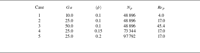
In our previous study (Xia et al. Reference Xia, Lin, Guo and Yu2024), DNS of clustered particle sedimentation in a fully periodic domain of size [
 $L_x$
,
 $L_y$
,
 $L_z$
] = [
 $320d_p$
,
 $10d_p$
,
 $80d_p$
] (see figure 12) were conducted. The gravitational acceleration
 $\boldsymbol{g}$
points to the negative
 $x$
direction. The intrinsic particle mesoscale structures in such a system differ significantly from those in fluidised beds, making it meaningful to examine whether the proposed models are applicable to this system. An overview of the cases used is provided in table 2, and the solid-to-gas density ratio is
 $\rho _r=100$
.
Parameter settings for the clustered particle sedimentation cases (Xia et al. Reference Xia, Lin, Guo and Yu2024). Here
 $\langle \phi \rangle$
denotes the domain-averaged solid volume fraction.

Snapshot for the large-scale PR-DNS of clustered particle sedimentation.

We evaluate the proposed models using the DNS data. As illustrated in figure 13, the predictions of the dissipation term model, the Reynolds stress interfacial term model and the dissipation rate interfacial term model are in good agreement with the corresponding DNS data. This consistency demonstrates that the submodels in the second-moment closure framework maintain their validity and accuracy for the clustered particle sedimentation system. Figure 14 presents a comparison between the predicted and actual values of the subgrid TKE and the velocity variance, in an attempt to assess the algebraic models for the particle-induced subgrid TKE (4.4) and the velocity variance (4.26). Good agreement between the predictions and the DNS data in figure 14 indicates that the proposed models may be applicable to various inhomogeneous particle-laden flows. The underestimation of
 $\widetilde {u^{\prime}_3u^{\prime}_3}$
may be attributed to the difference in boundary conditions: the model is established from the data of a fluidised bed with no-slip walls in the
 $z$
direction, whereas the test problem is the particle sedimentation in a fully periodic domain with a different particle clustering structure.
Parity plots between the actual and predicted values of gas-phase velocity variance: (a) dissipation term
 $\epsilon _{11}$
and (b) interfacial term
 $I_{11}$
. All values are normalised by
 $\rho {u}_{t}^3/d_p$
. (c) Dissipation rate interfacial term
 $I_{\epsilon }$
, with values normalised by
 $\rho {u}_{t}^4/d^2_p$
.


5. Conclusions
In this work, we have proposed a new model of the particle-induced subgrid TKE for an inhomogeneous fluidised bed by using DNS data and decomposing the total TKE into the homogeneous part, for which the model of Mehrabadi et al. (Reference Mehrabadi, Tenneti, Garg and Subramaniam2015) is employed, and the inhomogeneous part, which is modelled with the filtered fluid strain rate (Schneiderbauer Reference Schneiderbauer2017).
We have demonstrated that the second-moment models including the models for the dissipation, pressure–strain and interfacial terms in the Reynolds stress equation and the interfacial term in the dissipation rate equation, originally developed for homogeneous systems (Xia et al. Reference Xia, Yu, Lin and Guo2022a ), remain valid for the inhomogeneous system, provided that the mesoscale (inhomogeneous) drag and particle-induced TKE models are used for the dissipation rate interfacial term. The key feature of our Reynolds stress model is that when the particle effect vanishes, our model reduces to the single-phase model, and when the background turbulence is absent, our model can predict the particle-induced pseudo-turbulence.
We have extended the existing algebraic model (Ma et al. Reference Ma, Lucas and Bragg2020a ) for the velocity variance to inhomogeneous gas–solid flows by incorporating the effects of the filtered strain rate.
We have shown that the above inhomogeneous models based on the DNS data of the bubbling fluidised bed are applicable to clustered particle sedimentation in a periodic domain.
We believe that this study provides important insights into turbulence modelling for inhomogeneous particle-laden flows. We plan to implement the new models in the solver of the TFM in which the solid-phase equations are also involved and then examine the performance of our models by comparing the predictions with experiments. While the present modelling focuses on the effects of the filtered rate-of-strain tensor and filter width, more advanced modelling strategies such as dynamic adjustment techniques and data-driven approaches including artificial neural networks may be used to further improve model accuracy and generalisability in future studies.
Funding
The work was supported by the National Natural Science Foundation of China (grant nos. 12332015, 12302340 and 12072319) and the Natural Science Foundation of Zhejiang Province (LZ23A020006).
Declaration of interests
The authors report no conflict of interest.
Appendix A. Comparison of particle average vertical velocity
In this appendix we provide a comparison between the current PR-DNS results and the experimental data of Müller et al. (Reference Müller, Holland, Sederman, Scott, Dennis and Gladden2008) on the time-averaged particle vertical velocity profiles at two different heights above the bed bottom, for the case of
 $u_{in}=0.9$
m s−1, as shown in figure 15. The PR-DNS results obtained by Luo et al. (Reference Luo, Tan, Wang and Fan2016) using the immersed boundary method are also included for reference. We note that the grid resolution in the present work (
 $d_p/\Delta x$
= 25.6) is finer than that used in Luo et al. (Reference Luo, Tan, Wang and Fan2016) (
 $d_p/\Delta x$
= 12), enabling more accurate computations of TKE and dissipation rates.
Comparison of the time-averaged particle vertical velocities along the
 $z$
direction at heights of (a)
 $x=15$
mm and (b)
 $x=25$
mm in a bubbling fluidised bed (
 $u_{in}=0.9$
m s−1), with reference to existing experimental and numerical data.

The results in figure 15 show that particles move upward in the central region of the bed and downward near the sidewalls on average. The present PR-DNS results are in good agreement with both experimental and previous simulation data, despite the difference in the boundary condition in the
 $y$
direction, as mentioned earlier.
Appendix B. Reynolds-stress and dissipation-rate budgets
We compute the terms on the right-hand side of the Reynolds stress equation (3.9), the TKE equation (3.10) and the dissipation rate equation (4.16) for the bubbling fluidised bed studied. As shown in figure 16, each term in the TKE and Reynolds stress equations is directly evaluated from the DNS data and subsequently bin-averaged for (
 $\overline {\phi _s}=0.05,\,{Re}_m=120$
) and (
 $\overline {\phi _s}=0.45,\,{Re}_m=30$
). The results reveal that both shear production and diffusion terms are relatively weak in comparison with the interfacial term. This highlights that turbulence production in the present bubbling gas–solid fluidised bed is primarily driven by interfacial momentum exchange between particles and gas, rather than by mean shear. For TKE, the dissipation term and the interfacial term nearly balance with each other:
 $I_k \approx \epsilon _k$
.
Budgets of (a,b) Reynolds stress and (c,d) TKE transport equations for (a,c) (
 $\overline {\phi _s}=0.05,\,{Re}_m=120$
) and (b,d) (
 $\overline {\phi _s}=0.45,\,{Re}_m=30$
). The error bars are given by measuring the standard deviation from the bin-averaged values. All values are normalised with
 $\rho | \boldsymbol{u}_{\textit{slip}}|^3/d_p$
.

Budget of dissipation rate transport for (a) (
 $\overline {\phi _s}=0.05,\,{Re}_m=120$
) and (b) (
 $\overline {\phi _s}=0.45,\,{Re}_m=30$
). The error bars are given by measuring the standard deviation from the bin-averaged values. All values are normalised with
 $\rho | \boldsymbol{u}_{\textit{slip}}|^4/d^2_p$
.

Figure 17 shows the terms in the dissipation rate equation (4.16) at (
 $\overline {\phi _s}=0.05,{Re}_m=120$
) and (
 $\overline {\phi _s}=0.45,{Re}_m=30$
). Here the unknown interfacial term
 $I_\epsilon$
is obtained from (4.16). The results also indicate that both
 $P^M_\epsilon$
and
 $D^M_\epsilon$
can be neglected at finite solid volume fractions and particle Reynolds numbers. Again, only the interfacial term and the dissipation term are important and balance with each other:
 \begin{equation} -{{C_{\epsilon 2}}\overline {\phi _g} \rho \frac {{{{\epsilon }^2}}}{k}}+I_{\epsilon } \approx 0. \end{equation}