1. Introduction
Granular media, including geomaterials (sand and geotextile fabric) and soft condensed matter (such as granular/porous materials), have long been used as appropriate shock mitigating materials for blast protective structures (Skews Reference Skews2001; Smith Reference Smith2010; Petel et al. Reference Petel, Jetté, Goroshin, Frost and Ouellet2011; Britan et al. Reference Britan, Shapiro, Liverts, Ben-Dor, Chinnayya and Hadjadj2013; Del Prete et al. Reference Del Prete, Chinnayya, Domergue, Hadjadj and Haas2013; Vivek & Sitharam Reference Vivek and Sitharam2019). Adequately evaluating the shock-mitigating potential of granular media in terms of the streamwise pressure drop will be beneficial for the design of protective structures, which requires thorough knowledge of the shock interaction with granular media (Ben-Dor et al. Reference Ben-Dor, Britan, Elperin, Igra and Jiang1997; Britan et al. Reference Britan, Ben-Dor, Elperin, Igra and Jiang1997; Ji, Li & Chen Reference Ji, Li and Chen2012; Frost Reference Frost2018; Gubin Reference Gubin2018; Pontalier et al. Reference Pontalier, Loiseau, Goroshin and Frost2018).
Substantial progress has been made with respect to understanding shock propagation through rigid and compressible granular and porous media (Levy et al. Reference Levy, Ben-Dor, Skews and Sorek1993; Skews, Atkins & Seitz Reference Skews, Atkins and Seitz1993; Ben-Dor et al. Reference Ben-Dor, Britan, Elperin, Igra and Jiang1997; Britan et al. Reference Britan, Ben-Dor, Igra and Shapiro2001, Reference Britan, Ben-Dor, Igra and Shapiro2006; Sugiyama et al. Reference Sugiyama, Ando, Shimura and Matsuo2019), the pressure build-up on the target wall placed downstream of porous media subjected to the head-on shock impingement (Ram & Sadot Reference Ram and Sadot2013, Reference Ram and Sadot2015; Ram, Ben-Dor & Sadot Reference Ram, Ben-Dor and Sadot2018), the dynamic response of solid skeletons (Eriksen et al. Reference Eriksen, Toussaint, Turquet, Måløy and Flekkøy2018) and the amplification effect arising from the compaction waves (Britan et al. Reference Britan, Ben-Dor, Elperin, Igra and Jiang1997), unsteady flows in the wake of transmitted waves (Mehta et al. Reference Mehta, Salari, Jackson and Balachandar2019b ; Osnes et al. Reference Osnes, Vartdal, Omang and Reif2020) and the effects of particle characteristics (Britan et al. Reference Britan, Ben-Dor, Igra and Shapiro2001; Osnes et al. Reference Osnes, Vartdal, Omang and Reif2019, Reference Osnes, Vartdal, Omang and Reif2020). Levy et al. were among the first to propose wave diagrams for shock transmission through granular media (Levy et al. Reference Levy, Ben-Dor, Skews and Sorek1993). Recently, other investigators have depicted a more complete picture of possible flow configurations (Ling et al. Reference Ling, Wagner, Beresh, Kearney and Balachandar2012; Regele et al. Reference Regele, Rabinovitch, Colonius and Blanquart2014). Specifically, an incident shock wave impinging head-on upon a granular medium results in reflected and transmitted pressure waves. The strength and nature of the reflected wave, whether it is a shock wave or an expansion fan, depend on the parameters such as the incident shock strength and the volume fraction of the particle bed (Mehta et al. Reference Mehta, Neal, Salari, Jackson, Balachandar and Thakur2018, Reference Mehta, Salari, Jackson and Balachandar2019b ; Osnes et al. Reference Osnes, Vartdal, Omang and Reif2019, Reference Osnes, Vartdal, Omang and Reif2020). Owing to the combination of the sudden contraction of the gas duct (Mehta et al. Reference Mehta, Neal, Salari, Jackson, Balachandar and Thakur2018), shock reflection, diffraction and focusing from the particles (Naiman & Knight Reference Naiman and Knight2007; Mehta et al. Reference Mehta, Neal, Jackson, Balachandar and Thakur2016) and drag-induced momentum exchange between the gases and the solid skeleton (Mehta et al. Reference Mehta, Salari, Jackson and Balachandar2019b ; Osnes & Vartdal Reference Osnes and Vartdal2021), the transmitted shock quickly decays, resulting in downstream pressure attenuation behind the particle bed. Meanwhile, a succession of reflected pressure waves travels upstream and eventually catches up with the main reflected wave. The upstream pressure gradually increases and converges to a steady value. As the transmitted wave attenuates, gas filtration increasingly becomes the dominant process for determining unsteady flows; therefore, the drag-related friction between gases and the solid skeleton slows down the flows and contributes to the build-up of the pressure gradient (Regele et al. Reference Regele, Rabinovitch, Colonius and Blanquart2014). Although shock transmission and gas filtration have long been identified as the primary processes of shock attenuation, fundamental understanding of the process coupling and transition is still lacking, let alone the quantification of their respective contributions in terms of the streamwise pressure drop.
Multiple experiments and numerical solutions have been carried out to reveal the effects contributing to shock attenuation through granular media (Regele et al. Reference Regele, Rabinovitch, Colonius and Blanquart2014; Mehta et al. Reference Mehta, Neal, Salari, Jackson, Balachandar and Thakur2018, Reference Mehta, Salari, Jackson and Balachandar2019b). Regele et al. (Reference Regele, Rabinovitch, Colonius and Blanquart2014) carried out two-dimensional (2-D) particle-resolved simulations of shock transmitted through a frozen particle cloud (Regele et al. Reference Regele, Rabinovitch, Colonius and Blanquart2014). They attributed the pressure drop behind the transmitted shock to the multiple shock reflections created from each shock–particle interaction as the shock traverses the cloud. In addition, they reported that the pressure at the trailing edge of the cloud continues to drop as unsteady wakes form behind each particle, increasing the drag and thereby further reducing the pressure. Mehta et al. (Reference Mehta, Neal, Salari, Jackson, Balachandar and Thakur2018) also correlated the weakening of the transmitted shock to the dissipation of energy due to the formation of shocklets and bow shocks inside the particle bed, as revealed by fully resolved three-dimensional (3-D) inviscid simulations of shock interactions with a random particle bed. A follow-up study (Mehta et al. Reference Mehta, Salari, Jackson and Balachandar2019b) elucidated the critical role played by the supercritical post incident-shock flow in weakening the transmitted shock.
The early stage of shock–particle interaction is dominated by inviscid mechanisms, whereas viscous effects become important once the shock front has travelled over the particle. Osnes et al. (Reference Osnes, Vartdal, Omang and Reif2020) highlighted the viscous effect on shock attenuation and reflection caused by the formation of boundary layers and vortical wakes behind individual particles by performing viscous simulations of fixed particle curtains using large-eddy simulations with a 3-D unstructured mesh. They reported that stronger shock attenuation occurs at a lower Reynolds number because viscous dissipation becomes significant. A non-dimensional variable known as the sight length, L s, was proposed to account for the effects of the geometric properties of the particle cloud in terms of the particle size, volume fraction and regularity of the particle distribution (Osnes et al. Reference Osnes, Vartdal, Omang and Reif2019). Although L s was found to be able to characterize shock attenuation, its applicability is most likely limited because the derivation of L s is based on numerical simulations with the volume fraction in the dilute-to-dense transition (φ p ∼ 0.05–0.1) and a narrow variation range of particle diameters (d p ∼ 50–100 μm). Recently, particle-resolved simulations of shock interactions with movable particle clusters (Mehta et al. Reference Mehta, Goetsch, Vasilyev and Regele2022; Takahashi et al. Reference Takahashi, Nagata, Mizuno, Nonomura and Obayashi2022) have provided insights into the influences of particle motion on shock transmission and induced flows.
The particle-resolved simulations depict the flows around individual particles, facilitating the understanding of the underlying shock–particle interaction physics and the development of particle drag closure models (Osnes & Vartdal Reference Osnes and Vartdal2021). However, owing to the relatively small number of particles (N ∼ 10–100) and moderate particle volume fraction (φ p < 0.1–0.2), only minimum or weak shock attenuation is observed (Mehta et al. Reference Mehta, Neal, Jackson, Balachandar and Thakur2016, Reference Mehta, Neal, Salari, Jackson, Balachandar and Thakur2018; Osnes et al. Reference Osnes, Vartdal, Omang and Reif2019). More importantly, reproducing the takeover of the filtration process in the long particle bed is almost beyond the computational capacity of the particle-resolved simulation.
Shock attenuation through long and dense granular media (φ p p 0.01) is often assessed via either experiments (Ben-Dor et al. Reference Ben-Dor, Britan, Elperin, Igra and Jiang1997; Britan et al. Reference Britan, Ben-Dor, Elperin, Igra and Jiang1997, Reference Britan, Ben-Dor, Igra and Shapiro2001, Reference Britan, Shapiro and Ben-Dor2007; Lv et al. Reference Lv, Wang, Zhang and Li2018; Daniel & Wagner Reference Daniel and Wagner2022) or unresolved particle simulations (Ling et al. Reference Ling, Wagner, Beresh, Kearney and Balachandar2012; Sugiyama et al. Reference Sugiyama, Ando, Shimura and Matsuo2019). Laboratory experiments are predominantly carried out using shock tubes, wherein the planar shock front impinges upon packed particle columns consisting of grains with different particle sizes (Bakken et al. Reference Bakken, Slungaard, Engebretsen and Christensen2003), particle shapes (Lv et al. Reference Lv, Wang, Zhang and Li2018) and various granular materials (potash, polystyrene, nylon, glass, sand, steel, ceramic, etc.) (Levy et al. Reference Levy, Ben-Dor, Skews and Sorek1993; Ben-Dor et al. Reference Ben-Dor, Britan, Elperin, Igra and Jiang1997; Britan et al. Reference Britan, Ben-Dor, Igra and Shapiro2001). Pressure traces measured upstream, inside and downstream of the particle beds allow the establishment of complete transient pressure profiles from which the respective contributions from the transmitted wave and gas filtration can be identified (Britan et al. Reference Britan, Ben-Dor, Igra and Shapiro2006, Reference Britan, Shapiro and Ben-Dor2007). One of the most striking findings from the experiments is the empirical correlation between the attenuation coefficient, Ka, and a key dimensionless parameter known as the filter characteristic, θ (Bakken et al. Reference Bakken, Slungaard, Engebretsen and Christensen2003). Specifically, Ka is defined as the ratio between the downstream pressure (P DI) and the upstream pressure behind the incident shock, P 2, Ka = P DI/ P 2. Here θ is defined as
 \begin{equation} \theta =f_{m}\, \frac{\phi _{p}}{1-\phi _{p}}\, \frac{L_{0}}{d_{p}},\end{equation}
Variation of the Ka with the θ attained from a variety of shock-tube-based experiments reported in the literature denoted by scattered symbols. The experimental conditions are listed in table 1 in Appendix A. Two solid curves represent the supposed lower and upper limits of the Ka–θ correlations. Inset: typical experimental data with horizontal and vertical error bars indicating the uncertainties of Ka and θ, respectively.

where L 0 is the length of the particle bed, dp is the particle diameter, and fm is given by the classical Ergun equation (Ergun Reference Ergun1952)
 \begin{equation} f_{m}=\frac{\alpha }{{Re}_{m}}+\beta,\end{equation}
with two coefficients, α and β. The Rem in (1.2) is the modified Reynolds number accounting for the φ p effect,
 \begin{equation} {Re}_{\it m}=\frac{Re}{\phi _{p}}=\frac{\rho_{2}u_{2}{d}_{p}}{\mu_{2}\phi_{p}},\end{equation}
where ρ 2, u 2 and μ 2 are the density, velocity and dynamic viscosity, respectively, of the gases behind the incident shock. Bakken et al. (Reference Bakken, Slungaard, Engebretsen and Christensen2003) argued that for shock waves, Rem will always be so high that the fm converges to β, varying from 1.0 (for spheres) to 2.5 (crushed/angular particles). Hence, θ is reduced to
 \begin{equation} \theta =\beta \, \frac{\phi _{p}}{1-\phi _{p}}\, \frac{L_{0}}{{d}_{p}}.\end{equation}
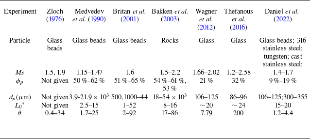
On the basis of a comprehensive literature review (Zloch Reference Zloch1976; Medvedev Reference Medvedev and Gelfand B.E.1990; Britan et al. Reference Britan, Ben-Dor, Igra and Shapiro2001; Bakken et al. Reference Bakken, Slungaard, Engebretsen and Christensen2003; Wagner et al. Reference Wagner, Beresh, Kearney, Trott, Castaneda, Pruett and Baer2012; Theofanous, Mitkin & Chang Reference Theofanous, Mitkin and Chang2016; Daniel & Wagner Reference Daniel and Wagner2022), figure 1 shows the Ka obtained from a variety of experiments plotted versus θ which ranges from O(10−1) to O(102), indicating an evident decreasing θ dependence of Ka. It is worth noting that there exist a level of uncertainties for both Ka and as indicated in the inset of figure 1. The uncertainties of Ka arise from the relatively poor repeatability and measurement errors while the uncertainties of θ are mainly caused by the variances of particle shape and size. As seen in figure 1, although a major proportion of the data falls into a band delimited by two curves, Ka = 1/(1+ θ) and Ka = 1/(1+ θ/6), a fraction of the outliers reside distinctly outside the concentrated band (Wagner et al. Reference Wagner, Beresh, Kearney, Trott, Castaneda, Pruett and Baer2012; Theofanous et al. Reference Theofanous, Mitkin and Chang2016; Daniel & Wagner Reference Daniel and Wagner2022). Specifically, these outliers exhibit distinctively different Ka values, but their θ values remain similar. Close examination of these outliers reveals that the corresponding experiments employed thin particle layers with moderate volume fractions. Although these cases have similar θ values suggesting similar Ka values according to the Ka–θ scaling law, incident shocks with varying strengths (M s ∼ 1.4–1.7) are sufficient to yield appreciable variability in Ka. The emergence of these apparent outliers arises from the fact that the Ka–θ scaling law cannot adequately account for the induced flows that mediate the interphase momentum transfer. The Ergen equation used to determine θ implies that the induced flows are solely controlled by gas filtration, meaning that the friction dissipation of the shock energy is predominantly responsible for the shock attenuation. Hence the Ka–θ scaling law fails to account for attenuation mechanisms involving complex shock dynamics, and the sudden reduction in the propagation area is associated with the presence of a solid phase, which is significant for thin particle layers with moderate volume fractions.
A deeper issue with using θ as the sole parameter to model the Ka data are the inconsistency between the physical meaning of fm and its simplified formulation (1.2) derived from fitting the experimental data. The physical meaning of fm is the scaled pressure drop across the length of the particle bed (Bakken et al. Reference Bakken, Slungaard, Engebretsen and Christensen2003)
 \begin{equation} f_{m}=\frac{\Delta P}{\rho_{2}u_{2}^{2}}\, \frac{{d}_{p}}{L_{0}}\, \frac{\left(1-\phi _{p}\right)^{3}}{\phi _{p}}=\frac{P_{2}-P_{DI}}{\rho_{2}u_{2}^{2}}\, \frac{{d}_{p}}{L_{0}}\, \frac{\left(1-\phi_{p}\right)^{3}}{\phi_{p}},\end{equation}
where the upstream pressure of the particle bed is assumed to be P 2. Substituting (1.5) into (1.1), we have
 \begin{equation} \theta =\frac{P_{2}-P_{DI}}{\rho _{2}u_{2}^{2}}\, \left(1-\phi _{p}\right)^{2}.\end{equation}
Clearly, the θ expressed in (1.6) is devoid of the influence of d p /L and is inconsistent with (1.4). It is problematic to use an empirical expression of f m, which has a specific physical bearing, to devise a key non-dimensional parameter.
To establish a proper scaling law of K a, which manifests the underlying shock attenuation mechanisms, it is necessary to understand the shock-induced unsteady flows through granular media, which vary from one shock/granular medium combination to another. To this end, we carried out several unresolved simulations of shock interactions with fixed particle beds via compressible computational fluid mechanics (CFD) coupled with the discrete parcel method (CCFD-DPM) (Ling et al. Reference Ling, Wagner, Beresh, Kearney and Balachandar2012; Sugiyama et al. Reference Sugiyama, Ando, Shimura and Matsuo2019; Tian et al. Reference Tian, Zeng, Meng, Chen, Guo and Xue2020). By varying the incident shock strength (M s ), particle volume fraction (φ p ), mean particle diameter (d p ) and length of the particle bed (L 0), we reproduced a variety of induced flows ranging from transmitted shock-dominated to transmitted shock- and gas-filtration collectively dominated and then to gas-filtration-dominated. Alongside the transition of the induced flow modes, the steady upstream and downstream pressures, P s,UI and P s,DI , undergo corresponding changes. The pressure also decreases. Therefore, the objective of this work is to construct the scaling laws of the P s,UI and P s,DI which are inspired by the physics underlying the transitions of unsteady flow modes.
The rest of this paper is organized as follows. In § 2, we introduce the CCFD-DPM numerical method and the prototypal configuration of the shock interaction with the particle bed. The CCFD-DPM generates results that are consistent with those of the particle-resolved simulations with regard to the strength decay of the transmitted shocks. The resulting shock attenuation effects in terms of the induced flows and the obtained P s,UI and P s,DI are described in § 3. The scaling laws of P s,UI and P s,DI are established on the basis of a non-dimensional parameter χ * which manifests the underlying attenuation mechanisms. The implications of the theoretical predictions P s,UI and P s,DI with respect to the estimation of particle shock dispersion are highlighted in § 4. Finally, the results are summarized in § 5.
2. Numerical method
2.1. Governing equations and numerical algorithm
Numerical simulations were performed based on CCFD-DPM, a Euler–Lagrange (E-L) numerical approach suitable for modelling of gas–particle flows in laboratory-scale systems (Sundaresan, Ozel & Kolehmainen Reference Sundaresan, Ozel and Kolehmainen2018; Koneru, Rollin & Durant Reference Koneru, Rollin and Durant2020; Tian et al. Reference Tian, Zeng, Meng, Chen, Guo and Xue2020). The CCFD-DPM approach tracks and accounts for particle–particle contact interactions.
For the gas phase, the volume-averaged governing equations (2.1)–(2.3) constructed in the Eulerian frame are based on a five-equation transport model, i.e. a simplified form of the Baer–Nunziato model, which has been modified to account for compressible multiphase flows ranging from dilute to dense gas–particle flows (Baer & Nunziato Reference Baer and Nunziato1986):
 \begin{equation} \frac{\partial \left(\phi _{f}\left\langle \rho _{f}\right\rangle \right)}{\partial t}+\nabla \cdot \left(\phi _{f}\left\langle \rho _{f}\right\rangle \tilde{\boldsymbol{u}}_{f}\right)=0,\end{equation}
 \begin{equation} \begin{array}{l} \frac{\partial \left(\phi _{f}\tilde{\boldsymbol{u}}_{f}\left\langle \rho _{f}\right\rangle \right)}{\partial t}+\nabla \cdot \left(\phi _{f}\left\langle \rho _{f}\right\rangle \tilde{\boldsymbol{u}}_{f}\tilde{\boldsymbol{u}}_{f}+\phi _{f}\left\langle P_{f}\right\rangle \right)\\[8pt] =\left\langle P_{f}\right\rangle \nabla \phi _{f}+\sum _{i}\left\{\phi _{p,i}\rho _{p,i}D_{p,i}\left(\tilde{\boldsymbol{u}}_{p,i}-\left(\tilde{\boldsymbol{u}}_{f}\right)_{i}\right)\right\}, \end{array}\end{equation}
 \begin{equation} \begin{array}{l} \frac{\partial \left(\phi _{f}\left\langle \rho _{f}\right\rangle \tilde{E}_{f}\right)}{\partial t}+\nabla \cdot \left(\phi _{f}\left\langle \rho _{f}\right\rangle \tilde{E}_{f}\tilde{\boldsymbol{u}}_{f}+\phi _{f}\left\langle p_{f}\right\rangle \tilde{\boldsymbol{u}}_{f}\right)\\[10pt] =\left\langle P_{f}\right\rangle \nabla \phi _{f}\cdot \tilde{\boldsymbol{u}}_{p}+\sum _{i}\left\{\phi _{p,i}\rho _{p,i}D_{p,i}\left(\boldsymbol{u}_{p,i}-\left(\tilde{\boldsymbol{u}}_{f}\right)_{i}\right)\cdot \tilde{\boldsymbol{u}}_{p,i}\right\}. \end{array}\end{equation}
The gas volume fraction, density, velocity, pressure and total energy of the gas are represented by φ
f
,
u
f
, ρ
f
, P
f
and E
f
, E
f
= ρ
f
e
f
+ 0.5 ρ
f
u
f
, respectively. In (2.1)–(2.3),
 $\langle \rangle$
and
 $\tilde{}$
denote phase-averaged and mass-averaged variables, respectively. Here ρ
p.i.
and
u
p,i
are the density and velocity of particle i, D
p,i
is the drag coefficient of particle i, and φ
p.i
= w
i,f
V
p,i
/V
f
is the contribution of particle i to the weighted particle volume fraction (w
i,f
is the distributed weight that particle i contributes to the particle volume fraction in fluid cell f, and V
p,i
and V
f
are the volumes of particle i and the fluid cell).
The corresponding gas–particle coupling drag force is calculated using (2.4), and D p,i can be expressed in the form of (2.5). Here sg is the specific weight of an individual particle with fluid, and r p is the particle radius. Here C d is the drag force coefficient, as shown in (2.6). This nonlinear drag force model is widely used in the numerical calculation of the interaction between shock waves and particle curtains and can consider the effects of the particle Reynolds number, Re p , φ p and Mach number, M a . Thus, C d is a function of Re p , φ p and M a :
 \begin{equation} F_{Drag}=\frac{1}{8}\pi d_{p}^{2}C_{d}\left(Re_{p},M_{a},\phi _{p}\right)\rho _{f}\left| \boldsymbol{u}_{f}-\boldsymbol{u}_{p,i}\right| \left(\boldsymbol{u}_{f}-\boldsymbol{u}_{p,i}\right) \end{equation}
 \begin{equation} D_{p,i}=\frac{F_{Drag}}{m_{p}\left(\boldsymbol{u}_{f}-\boldsymbol{u}_{p,i}\right)}=\frac{3}{8sg}C_{d}\left(Re_{p},M_{a},\phi _{p}\right)\frac{\left| \boldsymbol{u}_{f}-\boldsymbol{u}_{p,i}\right| }{r_{p}},\end{equation}
 \begin{equation} C_{d}\left(Re_{p},M_{a},\phi _{p}\right)=C_{d,std}\left(Re_{p}\right)\xi _{1}\left(Re_{p},M_{a}\right)\xi _{2}\left(\phi _{p}\right).\end{equation}
The particle Reynolds and Mach numbers are defined as
 \begin{equation} {Re}_{p}=\frac{\rho _{f}\left| \boldsymbol{u}_{f}-\boldsymbol{u}_{p}\right| {d}_{p}}{\mu },\quad M_{a}=\frac{\left| \boldsymbol{u}_{f}-\boldsymbol{u}_{p}\right| }{c},\end{equation}
where μ is the dynamic viscosity of the fluid and c is the local speed of sound of the fluid. The drag force model introduces the effects of the Mach number and particle volume fraction by correcting the standard drag correlation C d, which was developed by Clift & Gauvin (Reference Clift and Gauvin1970) using the Mach number multiplication factor (Parmar, Haselbacher & Balachandar Reference Parmar, Haselbacher and Balachandar2010) ξ 1 and the particle volume fraction multiplication factor (Sangani, Zhang & Prosperetti Reference Sangani, Zhang and Prosperetti1991) ξ 2, as follows:
 \begin{equation} C_{d,std}=\frac{24}{Re_{p}}\left(1+0.15Re_{p}^{0.687}\right)+0.42\left(1+\frac{42500}{Re_{p}^{1.16}}\right)^{-1},\end{equation}
 \begin{equation} \xi _{1}\left({Re}_{p},M_{a}\right)=C_{d}\left({Re}_{p},M_{a}\right)/C_{d,std}\left({Re}_{p}\right),\end{equation}
 \begin{equation} \xi _{2}\left(\phi _{p}\right)=\frac{1+2\phi _{p}}{\left(1-\phi _{p}\right)^{3}}.\end{equation}
The particle phase is represented by discrete particles whose motion is governed by Newton’s second law,
 \begin{equation} \frac{{d}\boldsymbol{u}_{p,i}}{{d}t}=D_{p,i}\left(\boldsymbol{u}_{f}-\boldsymbol{u}_{p,i}\right)-\frac{1}{\rho _{p}}\nabla \left\langle P_{f}\right\rangle +\frac{1}{m_{p}}\sum _{j}\boldsymbol{F}_{C,ij},\end{equation}
 \begin{equation} \frac{{d}\boldsymbol{x}_{p,i}}{{d}t}=\boldsymbol{u}_{p,i},\end{equation}
where u p,i and x p,i are the velocity and displacement of particle i, respectively, and F C,ij represents the collision force between particles i and j.
A four-way coupling strategy was adopted to account for the momentum and energy transfer between gases and particles. Specifically, the particle drag force and the associated work were incorporated into the momentum and energy equations of the gas phase as the source terms. The particles are driven by the pressure gradient force, drag force and collision force between particles (2.13). A soft sphere model, represented by a linear-spring–dashpot model, was employed to model the collision force between particles. Hence, F C,ij consists of a repulsive force and a damping force
 \begin{equation} \boldsymbol{F}_{C,ij}=k_{n,p}\boldsymbol{\delta }_{n}-\gamma _{n,p}\boldsymbol{u}_{n,ij},\end{equation}
where k n,p and γ n,p are the stiffness and damping coefficients of the particles and δ n and u n,ij are the overlap and normal velocity differences between the particles in contact, respectively. Here γ n,p is a function of the particle restitution coefficient ε p ,
 \begin{equation} \gamma _{n,p}=-\frac{2\ln \varepsilon _{p}}{\sqrt{\pi ^{2}+\ln \varepsilon _{p}}}\sqrt{m_{p}k_{n,p}}.\end{equation}
To solve the equations governing the gases, the weighted essentially non-oscillatory scheme (Liu Reference Liu1994) was used to reconstruct the primary flow variables. A Riemann solver proposed by Harten, Lax and van Leer was used to obtain the intercell fluxes (Toro Reference Toro2009). The third-order Runge–Kutta method was applied for time integration. The equations describing the particle velocity and position were discretized by the velocity Verlet algorithm. Bilinear/trilinear interpolation functions were adopted to calculate the particle volume fraction and source terms on the Eulerian grids, as well as the fluid variables on Lagrangian particles. Numerical details about CCFD-DPM can be found in our previous works (Tian et al. Reference Tian, Zeng, Meng, Chen, Guo and Xue2020).
2.2. Verification of the numerical method
The CCFD-DPM framework has been validated against several benchmark experiments involving shock-driven particle-laden flows (Tian et al. Reference Tian, Zeng, Meng, Chen, Guo and Xue2020), such as Rogue’s experiments (Rogue et al. Reference Rogue, Rodriguez, Haas and Saurel1998), which investigated shock dissipation through particle curtains; experiments carried out by Britan et al. (Reference Britan, Ben-Dor, Igra and Shapiro2006), which assessed both the gaseous and solid pressures inside particle columns impinged head on by shocks; and experiments involving the shock-induced interfacial instability of granular media (Xue et al. Reference Xue, Du, Shi, Gan and Bai2018, Reference Xue, Shi, Zeng, Tian, Han, Li, Liu, Meng, Guo and Bai2020).
Since the 2-D configurations are used to investigate the shock attenuation effect in the present work, it is necessary to validate the 2-D CCFD-DPM modelling with the experiments and 3-D particle-resolved simulations involving shock propagation through particle layers. Specifically, Grinten et al. measured the pressure traces upstream of and inside a densely packed particle column placed against the close end of a shock tube (van der Grinten, van Dongen & van der Kogel Reference van der Grinten, van Dongen and van der Kogel1985). The schematic of the experimental set-up is shown figure 2(a). Figure 2(b) compares the pressure histories at different locations measured in the experiment (dashed line) and those derived from our 2-D simulations using a 2-D configuration presented in figure 2(a). A good agreement is evident in terms of the overall profiles of pressures.
(a) Schematic of the experimental set-up in which a normal shock with the Mach number M
s
= 1.155 head-on collides with a densely packed long particle column (φ
p
= 70 %, L
0 = 1895 mm, d
p
= 375
 $\unicode{x03BC}$
m) placed against the close end of the shock tube. Four pressure transducers (PA
–PD
) were used to measure pressure traces upstream of and inside the particle column. (b) Comparison of pressure histories at PA
–PD
obtained in the experiment and our 2-D simulations.

As to the shock interaction between the mobile particle layers, Theofanous et al. (Reference Theofanous, Mitkin and Chang2016) and Wagner et al. ( Reference Wagner, Beresh, Kearney, Trott, Castaneda, Pruett and Baer2012) carried out a series of experiments of shock impingements of thin particle curtains, which serve as a definitive set of validation cases for the pertinent numerical simulations. We performed corresponding 2-D simulations and obtained the unsteady flows as well as the particle dispersion behaviours. Figures 3(a,b) and 3(d,e) compare the numerically derived pressure histories upstream and downstream of particle curtain with the experimental results reported by Theofanous et al. and Wagner et al., respectively. Here the pressure is scaled via the post incident shock pressure,
(a,b,d,e) The numerically and experimentally derived pressure histories upstream and downstream of shock impinged thin particle curtains. (c,f) The numerically and experimentally derived trajectories of UI and DI of shock dispersed particle curtains. (a–c) Experimental results are extracted from the reference (Theofanous et al. Reference Theofanous, Mitkin and Chang2016) in which the main parameters of particle curtain are φ
p
= 32 %, L
0 = 23.2 mm, d
p
ranging from 860
 $\unicode{x03BC}$
m to 960
 $\unicode{x03BC}$
m; (d–f) experimental results are extracted from the reference (Wagner et al. Reference Wagner, Beresh, Kearney, Trott, Castaneda, Pruett and Baer2012) in which the main parameters of particle curtain are φ
p
= 21 %, L
0 = 1.5 mm, d
p
ranging from 106
 $\unicode{x03BC}$
m to 125
 $\unicode{x03BC}$
m. Here TS and RS represent the transmitted shock in the particle layers and the shock reflected off the upstream interface.

 \begin{equation} P^{*}=\frac{P-P_{1}}{P_{2}-P_{1}},\end{equation}
and the time is scaled via the time the incident shock takes to travel the length of particle bed, L 0:
 \begin{equation} \tau =\frac{t}{L_{0}/u_{s}}.\end{equation}
As seen in figure 3, our simulations are able to accurately capture the arrival times of the reflected shock (RS) and transmitted shock (TS) and provide pressure profiles consistent with the experimental measurements. Besides, our simulations also reproduce the same dispersion rates of particle curtain in terms of the trajectories of upstream and downstream interfaces (UI and DI).
Particle resolved direct numerical simulations are able to depict the overall shock-induced flows with particle scale details rather than pressure histories at several locations. Figure 4 shows the evolutions of streamwise mean pressure (figure 4 a,c) and velocity (figures 4 b and 4 d) profiles attained from 3-D particle-resolved viscous (Osnes et al. Reference Osnes, Vartdal, Omang and Reif2020) (figure 4(a,b) and inviscid simulations (Mehta et al. Reference Mehta, Neal, Salari, Jackson, Balachandar and Thakur2018) (figure 4 c,d). Here the velocity is scaled via post incident shock velocity, u 2:
Comparisons of the streamwise mean pressure and flow velocity profiles, P *(x/L 0) (a), U *(x/ L 0) (c), P *(x/d p ) (b) and U *(x/d p ) (d), at different times derived from the present 2-D (solid line), 3-D (dotted line) CCFD-DPM simulations and 3-D viscous, (a)–(b) (Osnes et al. Reference Osnes, Vartdal, Omang and Reif2020) and inviscid, (c)–(d) (Mehta et al. Reference Mehta, Neal, Salari, Jackson, Balachandar and Thakur2018) particle-resolved simulations (dashed line).

 \begin{equation} U^{*}=\frac{u}{u_{2}}.\end{equation}
In the viscous simulation (Osnes et al. Reference Osnes, Vartdal, Omang and Reif2020), a particle curtain with 30 layers of particles (φ
p
= 10 %, L
0/ d
p
= 30) consisting of immobile particles (d
p
= 34
 $\unicode{x03BC}$
m) are impinged by a normal incident shock with M
s
= 2.6. In the inviscid simulation, a stronger shock (M
s
= 3) head-on impinges a thinner particle curtain (L
0/ d
p
= 19) consisting of larger mobile particles (d
p
= 100 μm) while the initial volume fraction is kept consistent, φ
p
= 10 %.
The particle resolved simulations have the advantages of capturing the particle scale flow fluctuations, especially during the initial shock induced transient. A previous study (Ling et al. Reference Ling, Wagner, Beresh, Kearney and Balachandar2012) found that a sustained variation in flow characteristics (velocity, pressure, density) across the particle layers persists after the passage of transmitted shock. Also the length scale of this variation is of the order of the layer's thickness. Therefore, particle unresolved simulations using the particle-scale volume averaged homogeneous formulations of drag force suffice to adequately account for the streamwise variation of mean flows in the wake of transmitted shock. The mean pressure and velocity profiles derived from the 2-D (solid curves) and 3-D (dotted curves) CCFD-DPM simulations are superimposed in figure 4 in which the structural parameters of numerical configuration are identical to those used in the particle resolved simulations. Evidently, the advancing of the RS and TS as well as the profiles of pressure and velocity derived from either 2-D or 3-D CCFD-DPM simulations are consistent with those derived from the particle resolved simulations, further corroborating the validity of the current 2-D modelling in describing the shock induced unsteady flows upstream of, inside and downstream of dense particle layers.
Finally it is necessary to justify the capacity of the particle unresolved simulations in accounting for the shock attenuation effect by elucidating the partition of energy influx caused by the TS in particle resolved and unresolved methods. The primary difference in this regard arises from the origin and resolution of the attained particle-scale fluctuations, which are an integral part of the total kinetic energy (Mehta, Jackson & Balachandar Reference Mehta, Jackson and Balachandar2019a ). The particle-resolved method accounts for the particle-scale fluctuations arising from multiple factors, including the shock phenomenon at individual particles, interparticle interactions via particle wakes and viscous effects (Regele et al. Reference Regele, Rabinovitch, Colonius and Blanquart2014; Osnes et al. Reference Osnes, Vartdal, Omang and Reif2019, Reference Osnes, Vartdal, Omang and Reif2020; Mehta et al. Reference Mehta, Jackson and Balachandar2019a ,Reference Mehta, Neal, Salari, Jackson, Balachandar and Thakur b , Reference Mehta, Salari, Jackson and Balachandar2018). By contrast, the particle-unresolved method using Ergun-type drag models considers the particle-scale fluctuations through the variations in the local flow parameters (Re), particle size (d p ) and local volume fraction (φ p ) (Ling et al. Reference Ling, Wagner, Beresh, Kearney and Balachandar2012; Houim & Oran Reference Houim and Oran2016; Theofanous & Chang Reference Theofanous and Chang2017; Meng et al. Reference Meng, Zeng, Tian, Li, He and Guo2019; Sugiyama et al. Reference Sugiyama, Ando, Shimura and Matsuo2019). The resolution of the particle-scale fluctuations observed in unresolved simulations depends on the ratio between the grid length and the particle diameter as well as the algorithm related to the information exchange between the fluid and particle phases (Regele et al. Reference Regele, Rabinovitch, Colonius and Blanquart2014; Mehta et al. Reference Mehta, Neal, Salari, Jackson, Balachandar and Thakur2018). Here Re, d p and φ p are the dominating parameters of the unsteady flows after the initial shock-induced transient because the steady forces on the particles as a function of these variables become predominant shortly at this time (Sun et al. Reference Sun, Saito, Takayama and Tanno2005; Parmar et al. Reference Parmar, Haselbacher and Balachandar2011, Reference Parmar, Haselbacher and Balachandar2012). Although the particle-unresolved methods may underestimate the particle-scale fluctuations during the initial shock-induced transient due to the lack of unsteady forces, the shock attenuation can be adequately accounted for because it is associated primarily with the long-term unsteady flows after the passage of the transmitted shock. The study by Osnes et al. (Reference Osnes, Vartdal, Omang and Reif2019, Reference Osnes, Vartdal, Omang and Reif2020) revealed that the initial shock-induced transient is negligible compared with the time scale of shock attenuation.
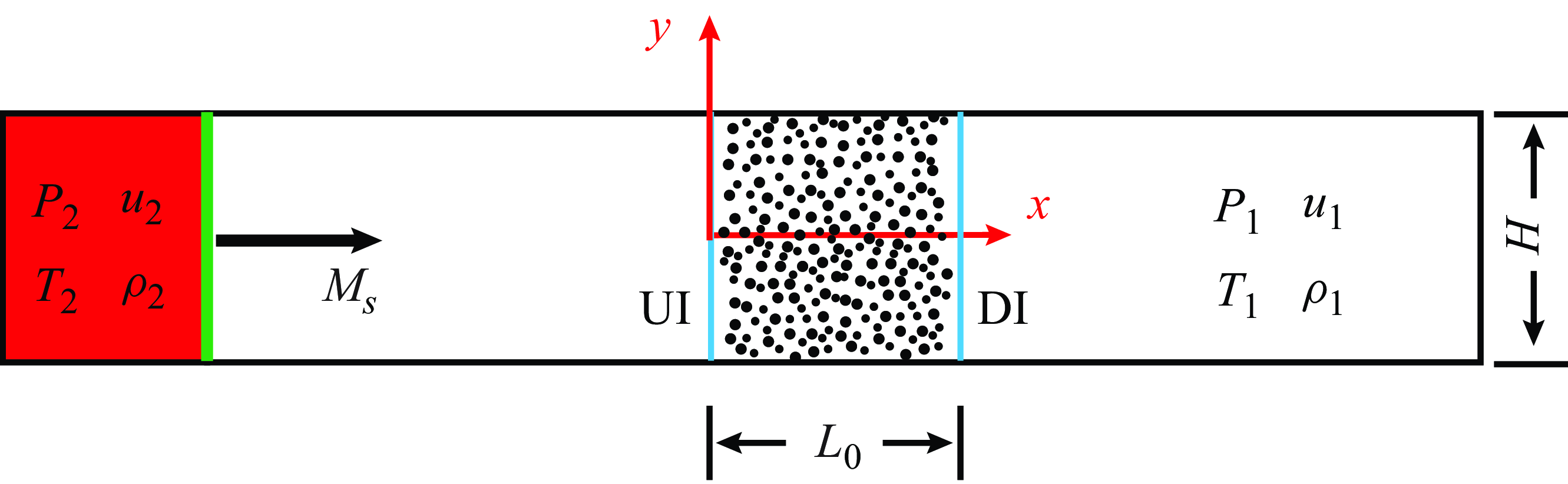
Computational configuration of a planar shock impinging head-on the UI of a fixed particle bed with a length of L 0. The ambient condition is imposed upon the DI of the particle bed.

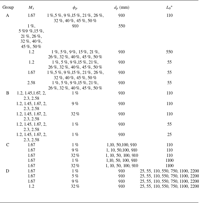
Distributions of numerical cases in the parameter spaces (M
s
, φ
p
) (a), (
 $\mathit{L}_{0}^{\mathrm{*}}$
, d
p
) (b) and (Re
p
, θ) (c).

2.3. Numerical set-up
The objective of this work is to obtain a fundamental understanding of the shock attenuation effect through granular media by proposing scaling laws for the upstream and downstream pressures rather than by precisely resolving these pressures. Hence, we consider the 2-D configuration shown in figure 5. A fixed particle bed consisting of randomly positioned/packed cylindrical particles is placed downstream of a planar incident shock (IS). Regele et al. noted that a proper 2-D numerical configuration can qualitatively capture the multidimensional behaviour of a real 3-D particle cloud impinged by an incident shock (Regele et al. Reference Regele, Rabinovitch, Colonius and Blanquart2014). The manageable cost of 2-D simulations allows us to investigate shock attenuation in a high-dimensional parameter space with variables spanning several decades. The computational domain upstream of the incident shock wave is long enough to ensure that no upstream disturbances influence the flows inside the particle bed during the computation duration. To minimize the variability of the streamwise mean flow parameters due to spanwise particle-scale fluctuations, the cross-sectional length of the fixed particle bed H is large enough, and periodic boundary conditions are used on the spanwise boundaries (y =
 $\pm$
H/2). Specifically, H ranges from 1100–110 d
p
as φ
p
increases from 0.01–0.5.
As indicated in the experimental and numerical studies (Britan et al. Reference Britan, Ben-Dor, Igra and Shapiro2001; Bakken et al. Reference Bakken, Slungaard, Engebretsen and Christensen2003; Osnes et al. Reference Osnes, Vartdal, Omang and Reif2019; Mehta et al. Reference Mehta, Salari, Jackson and Balachandar2019b
), the shock strength M
s
, the length of the particle bed
 $\mathit{L}_{0}^{\mathrm{*}}$
= L
0/d
p
, the particle diameter d
p
, and the volume fraction φ
p
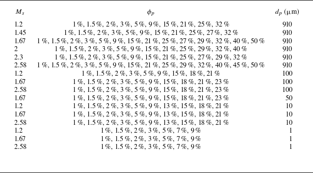
are the primary factors controlling shock attenuation. Hence, we devised 126 numerical cases with vastly varying M
s
,
 $\mathit{L}_{0}^{\mathrm{*}}$
, d
p
and φ
p
whose locations in the parameter spaces (M
s
, φ
p
) and (
 $\mathit{L}_{0}^{\mathrm{*}}$
, φ
p
) are shown in figures 6(a) and 6(b), respectively. Specifically, M
s
varies from 1.2–2.58; accordingly, the postincident shock flow varies from subsonic (M
2 = 0.29) to supersonic (M
2 = 1.23). The state of the particle layers ranges from moderately concentrated (φ
p
= 0.01) to dense (0.01< φ
p
<0.5) particle clouds and then to randomly close packed beds (φ
p
≥ 0.5). The mean values of the particle diameter, which obey a normal distribution (Δd
p
/d
p
= ±5.5 %), span three orders of magnitude and range from 1–910 μm. The length of the particle beds varies from dozens of particle layers (
 $\mathit{L}_{0}^{\mathrm{*}}$
= 25) to semi-infinite layers (
 $\mathit{L}_{0}^{\mathrm{*}}$
= 2200). The exact parameter values of each numerical case are listed in table 2 in Appendix A. The distributions of the numerical cases in the non-dimensional parameter space (Re
p
, θ) are plotted in figure 6
c). The θ ranges from O(10−1) to O(103), which is consistent with the range of θ variation observed in the previous experiments (figure 1). Thereafter, the numerical cases are denoted by the combination of four critical variables, i.e. C-M
s
-φ
p
-
 $\mathit{L}_{0}^{\mathrm{*}}$
-d
p
(in μm).
3. Numerical results
3.1. Transmission-dominated shock attenuation
Figure 7(a) shows a typical x–t diagram of the mean pressures P * averaged over the transverse direction in a moderately concentrated particle bed consisting of a handful of particle layers (1.67-0.01-110-910). The corresponding unsteady flows are dominated by various waves discerned from the numerical schlieren (figure 7 b), which is consistent with other investigations (Levy et al. Reference Levy, Ben-Dor, Skews and Sorek1993; Rogue et al. Reference Rogue, Rodriguez, Haas and Saurel1998; Ling et al. Reference Ling, Wagner, Beresh, Kearney and Balachandar2012; Regele et al. Reference Regele, Rabinovitch, Colonius and Blanquart2014). As the IS impinges on the UI of the particle bed, a part of it is transmitted into the bed as a TS, and another part is reflected, becoming the primary reflected shock (PRS). As the TS penetrates layers of particles, it bounces back and forth inside the interparticle pores, some of which find a way to emerge from the UI as weak compression waves (CWs). The CWs eventually catch up with the PRS, which hence becomes increasingly stronger. Moreover, the TS becomes increasingly dispersed with decreasing strength. When the TS emerges from the downstream interface (DI) of the particle bed at t = t TS , a downstream travelling contact surface (CS) is created, trailed by a later emerging contact surface (CS1) previously formed at the UI. Simultaneously, a reflected rarefaction wave (RRW) travels upstream. A steady pressure gradient is set up upon the RRW reaching the UI at t = t RRW.
(a) The x–t diagram of mean pressures P
*, (b) numerical schlieren, evolution of the P
* profiles in (c) the early and (d) late times, (e) temporal variations in pressures upstream (
 $P_{{UI}}^{\mathrm{*}}$
, X = 0) of, inside (P
*(X = 0.5)) and downstream (
 $P_{{DI}}^{\mathrm{*}}$
, X = 1) of particle bed for the case C-1.67-0.01-110–910. Note that the induced density ρ is scaled by ρ
2. The dashed curve in (d) represents the steady P
* profile predicted by the Morrison model with Δ
 $P_{{s}}^{\mathrm{*}}$
=
 $P_{{s},{UI}}^{\mathrm{*}}$
-
 $P_{{s}, {DI}}^{{*}}$
. Here PRS, primary reflected shock; CWs, compression waves; RRW, reflected rarefaction wave; CS1, contact surface formed at the UI; CS2, contact surface formed at the DI.

The evolution of the P
* profiles shown in figure 7(c) manifests the decay of the TS as well as the gradual increase in the upstream pressure due to the arrival of CWs. Specifically, the strength of the TS,
 $P_{TS}^{\mathrm{*}}$
, is defined as the pressure jump across its front, which decreases by 12 % after the TS penetrates 110 layers of particles while the propagation velocity remains largely constant. After tTS
, in the wake of RRW, the profile of P
*(X) converges to a steady
 $P_{{steady}}^{\mathrm{*}}$
(X), corresponding to a steady diffusional pressure field dictated by the pressure differential between the upstream and downstream directions, Δ
 $P_{s}^{{*}}$
=
 $P_{{s},{UI}}^{\mathrm{*}}$
-
 $P_{{s}, {DI}}^{{*}}$
(see figure 7d
). Note that
 $\mathit{P}_{{steady}}^{\mathrm{*}}$
(X) agrees well with the profile predicted by the Morrison model (Morrison Reference Morrison1972) with Δ
 $\mathit{P}_{{s}}^{\mathrm{*}}$
=
 $\mathit{P}_{{s},{UI}}^{{*}}$
-
 $\mathit{P}_{{s}, {DI}}^{{*}}$
. As shown in figure 7(e),
 $\mathit{P}_{{DI}}^{\mathrm{*}}$
jumps to
 $\mathit{P}_{{s}, {DI}}^{{*}}$
immediately after the TS emerges from the DI,
 $\mathit{P}_{{s}, {DI}}^{{*}}$
= 0.88, while
 $\mathit{P}_{{UI}}^{\mathrm{*}}$
gradually increases and converges to
 $\mathit{P}_{{s},{UI}}^{\mathrm{*}}$
at t = tRRS
,
 $\mathit{P}_{{s},{UI}}^{\mathrm{*}}$
= 1.72. In this scenario, the pressure drop in terms of Δ
 $\mathit{P}_{{s}}^{\mathrm{*}}$
clearly depends on the propagation of the TS, which is referred to as the transmission-dominated mode hereafter.
3.2. Transmission-filtration-dominated shock attenuation
For a denser and longer particle bed, the TS may not emerge from the UI of the bed, as indicated in figure 8. Although the x–t diagram of the streamwise mean pressure P
* (figure 8
a) shows a pattern similar to that in figure 7(a), no RRW can be identified from the numerical schlieren (figure 8
b), indicating complete dissipation of the TS midway through the bed. The evolution of the profiles of P
*(X) (figure 8c) demonstrates a rapid decay of the TS, which degrades into a compression wave when it travels to X = X
TS
= 0.67; therefore, no pressure jump across the TS front is discernible. Hereafter, the distance from the UI upon which the TS degrades into a transmitted compression wave (TCW) is referred to as the maximum transmission length,
 $\mathit{L}_{{TS}}^{\mathrm{*}}$
, which is a function of M
s
, φ
p
and d
p, as revealed below. The determination procedure of the
 $\mathit{L}_{{TS}}^{\mathrm{*}}$
is presented in Appendix B.
(a) The x–t diagram of mean pressures P
*, (b) numerical schlieren, evolution of the P
* profiles in in (c) the early and (d) times, (e) temporal variations in pressures upstream (
 $\mathit{P}_{{UI}}^{\mathrm{*}}$
, X = 0) of, inside (P
*(X = 0.5)) and downstream (
 $\mathit{P}_{{DI}}^{\mathrm{*}}$
, X = 1) of particle bed for the case C-1.67-0.01-1100-1. The dashed and dotted curves in (d) represent the steady pressure profiles predicted by the Morrison model with Δ
 $\mathit{P}_{{s}}^{\mathrm{*}}$
=
 $\mathit{P}_{5}^{\mathrm{*}}$
–
 $\mathit{P}_{1}^{\mathrm{*}}$
, Δ
 $\mathit{P}_{{s}}^{\mathrm{*}}$
=
 $\mathit{P}_{{s},{UI}}^{\mathrm{*}}$
–
 $\mathit{P}_{{s}, {DI}}^{{*}}$
, respectively.

As the TCW emerges from the DI, the downstream pressure
 $\mathit{P}_{{DI}}^{\mathrm{*}}$
slowly increases until the arrival of CS1 at τ =
 $\tau _{{\textit{CS}_{1}}}$
(figure 8
e). The
 $\mathit{P}_{{DI}}^{\mathrm{*}}$
eventually stabilizes at a value appreciably higher than the ambient pressure,
 $\mathit{P}_{{s}, {DI}}^{{*}}$
= 0.35, contradicting the previously held assumption that
 $\mathit{P}_{{s}, {DI}}^{{*}}$
remains ambient if no TS emerges. As described in Appendix C, the noticeable increase in
 $\mathit{P}_{{DI}}^{\mathrm{*}}$
is associated with the thermodynamic evolution of heated gases between CS1 and CS2 flowing through the DI. Moreover, the upstream pressure
 $\mathit{P}_{{UI}}^{\mathrm{*}}$
(τ) (figure 8
e) undergoes a sharp jump followed by a gradual increase, converging to
 $\mathit{P}_{{s},{UI}}^{\mathrm{*}}$
= 2.96 at late times. Notably, the increase in
 $\mathit{P}_{{UI}}^{\mathrm{*}}$
does not completely cease when the last CW (CW
T
) starting from X
TS
reaches the UI at τ
CWT = 1.95. Rather, we observe a persistent increase in
 $\mathit{P}_{{DI}}^{\mathrm{*}}$
, which lasts until CS1 emerges from the DI at τ
CS1 = 6.6. The fast-flowing interstitial gases swept by the CW
T
continue to be slowed down by friction between gases and the solid skeleton, thereby generating compression waves that can also emerge from the UI and further increase
 $\mathit{P}_{{DI}}^{\mathrm{*}}$
. The overall pressure profile becomes steady upon τ
CS1,
 $\mathit{P}_{{s}}^{\mathrm{*}}(\mathit{X})$
, which is consistent with Morrison’s prediction for
 $\mathit{P}_{{s},{UI}}^{\mathrm{*}}$
= 2.96 and
 $\mathit{P}_{{s}, {DI}}^{{*}}$
= 0.35, as shown in figure 8(d). Since the pressure drop in this scenario depends on both the TS and the gas filtration, this type of shock attenuation is referred to as the transmission-filtration-dominated mode.
3.3. Filtration-dominated shock attenuation
The TS can barely survive a few layers of particles when the IS penetrates a densely packed particle bed, as observed in the case of C-1.67-0.5-110-910. Hence, gas filtration takes over and becomes the dominant process. A typical diffusional pressure field develops alongside the gas filtration through the bed, as shown in figure 9(a), and a steady flow field forms after CS1 emerges from the DI (figure 9
b). The friction between gases and the rigid skeleton slows down the induced flows (figure 9c), resulting in a gradual build-up of gaseous pressure (figure 9
d). Moreover, the upstream travelling compression waves caused by the slowing down of induced flows give rise to a slow but persistent increase in
 $\mathit{P}_{{UI}}^{\mathrm{*}}$
after the sharp jump at the PRS (figure 9
g). Eventually,
 $\mathit{P}_{{UI}}^{\mathrm{*}}$
converges to a
 $\mathit{P}_{{s},{UI}}^{\mathrm{*}}$
slightly lower than the pressure after the shock wave is reflected off a solid surface known as
 $\mathit{P}_{5}^{\mathrm{*}}$
. In the case of C-1.67-0.5-110-910,
 $\mathit{P}_{{s},{UI}}^{\mathrm{*}}$
= 3.29 while
 $\mathit{P}_{5}^{\mathrm{*}}$
= 3.38.
(a) The x–t diagram of mean pressures P
*, (b) numerical schlieren, (c–f) profiles of (c) V
*(X), (d) P
*(X), (e) T
*(X), (f) ρ
*(X), (g) temporal variations in pressures upstream (
 $\mathit{P}_{{UI}}^{\mathrm{*}}$
, X = 0), inside (P
*(X = 0.5)) and downstream (
 $\mathit{P}_{{DI}}^{\mathrm{*}}$
, X = 1) of the particle bed for the case C-1.67-0.5-110-910. The dashed and dotted curves in (d) represent the steady pressure profiles predicted by the Morrison model with Δ
 $\mathit{P}_{{s}}^{\mathrm{*}}$
=
 $\mathit{P}_{5}^{\mathrm{*}}$
–
 $\mathit{P}_{1}^{\mathrm{*}}$
and Δ
 $\mathit{P}_{{s}}^{\mathrm{*}}$
=
 $\mathit{P}_{{s},{UI}}^{\mathrm{*}}$
–
 $\mathit{P}_{{s}, {DI}}^{{*}}$
, respectively. The temperature and velocity are scaled by T
2 and u
2, respectively.

In contrast with the isothermal filtration assumption of the conventional filtration model, shock-induced filtration may exhibit pronounced non-isothermal effects, as explored in our previous work (Li, Zeng & Xue Reference Li, Zeng and Xue2023). The scaled temperature profiles, T
*(X), shown in figure 9(e) indicate an intensely heated gas band confined in CS1 and CS2 traversing the bed, resulting in a non-monotonic variation in the gaseous density, ρ
*(X) (figure 9
f). The downstream gas density,
 $\rho _{{DI}}^{\mathrm{*}}$
, is also affected by the nozzling effect at the DI characterized by sudden acceleration as it approaches the DI (figure 9
f). As the heated gas band flows through the DI, the downstream pressure,
 $\mathit{P}_{{DI}}^{\mathrm{*}}$
, slowly increases to a steady value,
 $\mathit{P}_{{s}, {DI}}^{{*}}$
= 0.11 (figure 9
g). The evolution of
 $\mathit{P}_{{DI}}^{\mathrm{*}}$
due to the combination of the non-isothermal effect and the nozzling effect is elucidated in Appendix C. The diffusional pressure profile predicted by the Morrison model with
 $\mathit{P}_{{s},{UI}}^{\mathrm{*}}$
= 3.29 and
 $\mathit{P}_{{s}, {DI}}^{{*}}$
= 0.11 provides better agreement with the simulated result than the theoretical estimation with
 $\mathit{P}_{{s},{UI}}^{\mathrm{*}} = \mathit{P}_{5}^{\mathrm{*}}$
and
 $\mathit{P}_{{s}, {DI}}^{{*}} = \mathit{P}_{1}^{\mathrm{*}}$
= 0 (figure 9
d). Since
 $\mathit{P}_{{s},{UI}}^{\mathrm{*}}$
and
 $\mathit{P}_{{s}, {DI}}^{{*}}$
are associated with non-isothermal gas filtration, the shock wave attenuation in this scenario is referred to as the filtration-dominated mode.
3.4. Mode transition of shock wave attenuation
As mentioned in the previous sections, the mechanism governing shock attenuation undergoes a fundamental transition when the filtration process takes over the TS propagation. Accordingly, the shock attenuation effects in terms of the pressure drop, ΔP
* =
 $\mathit{P}_{{s},{UI}}^{\mathrm{*}}$
-
 $\mathit{P}_{{s}, {DI}}^{{*}}$
, ought to experience the mode transition. The most pronounced characteristic of the mode transition is the ratio between the maximum transmission length,
 $\mathit{L}_{{TS}}^{\mathrm{*}}$
, and the length of the particle bed,
 $\mathit{L}_{0}^{\mathrm{*}}$
, where χ =
 $\mathit{L}_{{TS}}^{\mathrm{*}}/\mathit{L}_{0}^{\mathrm{*}}$
. A transmission-dominated mode (Mode I) requires χ to be larger than one unit, χ >1, while the χ of the order of O(10−2) and below guarantees a filtration-dominated mode (Mode III). When χ is in between these values, a transmission-filtration-dominated mode (Mode II) prevails.
To accurately determine χ and the resulting shock attenuation mode for a specific combination of an IS and a particle bed, it is necessary to derive the corresponding
 $\mathit{L}_{{TS}}^{\mathrm{*}}$
. Figures 10(a) and 10(b) show the dependences of
 $\mathit{L}_{{TS}}^{\mathrm{*}}$
on φ
p
, where d
p
spans four orders of magnitude (figure 10
a) and the strength of the IS increases from weak (M
s
= 1.2) to strong (M
s
= 2.58) (figure 10
b). Here
 $\mathit{L}_{{TS}}^{\mathrm{*}}$
decreases dramatically with increasing φ
p
towards the lower limit of the φ
p
range. We observe a one-order-of-magnitude decrease in
 $\mathit{L}_{{TS}}^{\mathrm{*}}$
when φ
p
only increases by several per cent from the lower limit of the dense regime, φ
p
= 0.01. The decrease of
 $\mathit{L}_{{TS}}^{\mathrm{*}}$
is significantly slowed down when φ
p
exceeds 0.1. The
 $\mathit{L}_{{TS}}^{\mathrm{*}}$
converges to several particle layers when the particle bed approaches densely packed packing (φ
p
> 0.4), which is set by the resolution limit of the particle unresolved method. Although similar decaying dependences of
 $\mathit{L}_{{TS}}^{\mathrm{*}}$
on φ
p
evident despite the distinctively varying M
s
and d
p
, the decay rate of
 $\mathit{L}_{{TS}}^{\mathrm{*}}$
is most significant for particle beds consisting of small beads (d
p
= 1 μm) subject to a weak IS (M
s
= 1.2). We note that the d
p
effect becomes trivial as d
p
exceeds 100 μm.
Variations in the
 $\mathit{L}_{{TS}}^{\mathrm{*}}$
with the increasing φ
p
for particle beds with different d
p
(a) and subjected to the IS with different M
s
(b). The shaded bands in (a) encompass the results attained from cases with the same d
p
but different M
s
(M
s
∼ 1.2–2.58) while the shaded bands in (b) envelop the results attained from cases with the same M
s
but different d
p
(d
p
∼ 1–910
 $ \unicode{x03BC}$
m).

In previous studies on the transmission-dominated mode of shock attenuation (Osnes et al. Reference Osnes, Vartdal, Omang and Reif2019, Reference Osnes, Vartdal, Omang and Reif2020; Mehta et al. Reference Mehta, Salari, Jackson and Balachandar2019b ), the collective effects of the M s and d p shown in figure 9 were incorporated into the particle Reynolds number Re p . These studies reported a faster decay of TS with an increased Re p (Osnes et al. Reference Osnes, Vartdal, Omang and Reif2020). The product of the first two terms in the expression of θ (1.1), which is denoted as θ 1 as follows, explicitly accounts for the attenuation effects from φ p as well as Re p:
 \begin{equation} \theta _{1}=f_{m}\, \frac{\phi _{p}}{1-\phi _{p}}=\left(\frac{\alpha \phi _{p}}{{Re}_{p}}+\beta \right)\, \frac{\phi _{p}}{1-\phi _{p}}.\end{equation}
Figure 10(a) plots the numerically derived
 $\mathit{L}_{{TS}}^{\mathrm{*}}$
against θ
1 with α = 150 and β = 1 in double logarithmic coordinates. Clearly, θ
1 fails to scale the
 $\mathit{L}_{{TS}}^{\mathrm{*}}$
attained from a wide range of combinations M
s
, φ
p
and d
p, as indicated by considerable variabilities.
Another dimensionless variable that has the potential to scale
 $\mathit{L}_{{TS}}^{\mathrm{*}}$
is related to the filtration Reynolds number first introduced by Morrison (Reference Morrison1972),
 \begin{equation} {Re}_{f}=\frac{b}{a^{2}}\frac{P_{5}-P{1}^{}{}{}}{P_{1}}\, \frac{P_{1}\rho _{1}}{L_{0}\mu _{1}^{2}},\end{equation}
where subscripts 1 and 5 refer to the parameters of the downstream ambient gases and gases behind the reflected shock, respectively, and the Darcy, a, and Forchheimer, b, coefficients are functions of φ p and d p . For particle beds composed of spherical particles, a and b are expressed as
 \begin{equation} a = 180\frac{\phi _{p}^{2}}{\left(1-\phi _{p}\right)^{2}}\frac{1}{d_{p}^{2}},\end{equation}
 \begin{equation} b=1.8\frac{\phi _{p}}{1-\phi _{p}}\frac{1}{{d}_{p}}.\end{equation}
Substituting (3.3) and (3.4) into (3.2), we have
 \begin{equation} {Re}_{f}=\frac{1}{18000L_{0}^{*}}\, \frac{\left(P_{5}-P_{1}\right)}{P_{1}}\, \frac{\rho _{1}P_{1}d_{p}^{2}}{\mu _{1}^{2}}\, \frac{\left(1-\phi _{p}\right)^{3}}{\phi _{p}^{3}}.\end{equation}
Here Re
f
is found to underlie the transition of filtration-induced gas flow from viscous loss-dominated Darcy flow (Re
f
→0) to inertial loss-dominated Forchheimer flow (Re
f
→∞) (Britan, Shapiro & Ben-Dor Reference Britan, Shapiro and Ben-Dor2007). Hence, Re
f
is indicative of the nature of interphase friction, which is the predominant mechanism for the filtration-dominated mode of shock attenuation. Leaving out the first term involving
 $\mathit{L}_{0}^{\mathrm{*}}$
, the remainder of Re
f
constitutes a new dimensionless parameter, Re
f,1, which manifests the effects arising from M
s
(correlated with P
5), d
p
and φ
p:
 \begin{equation} {Re}_{f,1}=\frac{\left(P_{5}-P_{1}\right)}{P_{1}}\, \frac{\rho _{1}P_{1}d_{p}^{2}}{\mu _{1}^{2}}\, \frac{\left(1-\phi _{p}\right)^{3}}{\phi _{p}^{3}}.\end{equation}
The plot of
 $\mathit{L}_{{TS}}^{\mathrm{*}}$
against Re
f,1 in the double logarithmic coordinates is shown in figure 11(b), revealing a significant improvement in data convergence. The relative root mean square error (RRMSE) of all the numerically derived
 $\mathit{L}_{{TS}}^{\mathrm{*}}$
values from the linearly fitted master curve denoted by the black line in figure 11(b) is 5.6 %.
Variations in the
 $\mathit{L}_{{TS}}^{\mathrm{*}}$
with the increasing θ
1 (a) and Re
f,1 (b).

Inspired by θ 1 and Re f,1, which correlate with the attenuation mechanisms in the transmission- and filtration-dominated modes, respectively, we construct a dimensionless parameter composed of Re p and a power function of φ p as
 \begin{equation} \eta ={Re}_{p}\, \frac{\left(1-\phi _{p}\right)^{3}}{\phi _{p}^{4}}.\end{equation}
The correlations between η and θ 1 as well as Re f,1 are shown in figures 12(a) and 12(b), respectively. Clearly, there exists an explicit semilinear Re f,1 dependence of η in contrast with the scattering η corresponding to a given θ 1.
Variations in the η with the increasing θ 1 (a) and Re f,1 (b).

The variation in
 $\mathit{L}_{{TS}}^{\mathrm{*}}$
with η is shown in figure 13 in the double logarithmic coordinates. The majority of the data collapse into a narrow band centred on a linearly fitted master curve, yielding a satisfactorily small RRMSE of 4.1 %. Therefore, the master curve in figure 13 represents the scaling law for
 $\mathit{L}_{{TS}}^{\mathrm{*}}$
:
Variations in the
 $\mathit{L}_{{TS}}^{\mathrm{*}}$
with the increasing η.

 \begin{equation} \lg L_{{TS}}^{*}=0.29\lg \eta +0.22.\end{equation}
When η approaches zero, which occurs with extremely weak IS (Re
p
→0) and/or exceedingly small d
p
(Re
p
→0) and/or the most densely packed bed (φ
p
→1),
 $\mathit{L}_{{TS}}^{\mathrm{*}}$
converges to its lower limit, which is of the order of O(100). Note that φ
p
in (3.7) is for the 2-D system. Thus, for the 3-D bed, we should change φp,3-D
into its 2-D counterpart, φp,2-D
, using φp,2-D
≈ 1.22φp,3-D
.
Using the scaling law of
 $\mathit{L}_{{TS}}^{\mathrm{*}}$
(3.8), we can calculate the ratio between
 $\mathit{L}_{{TS}}^{\mathrm{*}}$
and
 $\mathit{L}_{0}^{\mathrm{*}}$
, i.e. χ, for all numerically and experimentally investigated shock attenuation systems, including the cases plotted in figure 1. An explicit correlation between χ and θ is shown in figure 14. As θ ranges from O(10−1) to O(103), χ varies from O(103) to O(10−2), whereby the shock attenuation crosses over all three modes. Notably, the χ values of systems whose θ values are very close vary enough so that they become quite distinguishable. Specifically, the χ of systems with θ ∼ 3 highlighted in figure 1 varies from 3.5 to 6.5. It is worth noting that whenever the results from 3-D configurations are compared with their 2-D counterparts, or vice versa, the 3-D volume fraction, φp,3-D
, ought to be converted into 2-D equivalent, φp,2-D
. Following the conversion principle proposed by Borchard-Ott (Reference Borchard-Ott2011), we adopt a the linear interpolation between the porosity at the maximum (hexagonal) and minimum (none particle) packing density states for monosized packing with disks (2-D) and spheres (3-D):
Variations in the θ with the increasing χ.

 \begin{equation} \phi _{{p},3D}=\phi _{{p},2D}\frac{\phi _{{p},3D}^{\textit{HCP}}-0}{\phi _{{p},2D}^{\textit{HCP}}-0}=\frac{0.74-0}{0.097-0}\phi _{{p},2D}=0.82\phi _{{p},2D}.\end{equation}
Hereafter, whenever the experimental data are plotted, their volume fraction would be converted to their 2-D equivalent according to (3.9).
3.5. Scaling laws for shock attenuation
To assess the key role played by the χ in the upstream and downstream pressures of the particle bed impinged by the IS of varying intensity, we plot the variations in
 $\mathit{P}_{{s},{UI}}^{\mathrm{**}}$
and
 $\mathit{P}_{{s}, {DI}}^{{*}}$
with χ in figures 15(a) and 15(d), respectively, wherein the symbols are rendered with the flow Mach number behind the IS, M
2. Here,
 $\mathit{P}_{{s},{UI}}^{\mathrm{**}}$
is scaled via
Variations in the
 $\mathit{P}_{{s},{UI}}^{\mathrm{**}}$
with the increasing χ (a), θ (c) and χ
* (e). Variations in the
 $\mathit{P}_{{s}, {DI}}^{{*}}$
with the increasing χ (b), θ (d) and χ
* (f).

 \begin{equation} P_{{s},{UI}}^{**}=\frac{P_{{s},{UI}}-P_{2}}{P_{5}-P_{2}},\end{equation}
where P
2 is the pressure behind the IS. Compared with the wide variations observed in the θ dependences of
 $\mathit{P}_{{s},{UI}}^{\mathrm{**}}$
(figure 15
b) and
 $\mathit{P}_{{s}, {DI}}^{{*}}$
(figure 15
e), the deviations of
 $\mathit{P}_{{s},{UI}}^{\mathrm{**}}$
(χ) and
 $\mathit{P}_{{s}, {DI}}^{{*}}$
(χ) from the fitted master curves are significantly reduced, with relative standard deviations of RRMSE
UI,χ
= 11 %, RRMSE
DI,χ
= 35 %.
Closer examination of the χ dependences of
 $\mathit{P}_{{s},{UI}}^{\mathrm{**}}$
in figure 15(a) reveals that
 $\mathit{P}_{{s},{UI}}^{\mathrm{**}}$
for systems with similar χ varies with M
2. Specifically, a system with a smaller M
2 yields a lower
 $\mathit{P}_{{s},{UI}}^{\mathrm{**}}$
than those with the same χ but a larger M
2. In fact, χ only indicates the nature of the shock-induced unsteady flows inside the granular media in terms of its location in the mode spectrum ranging from transmission-dominated to filtration-dominated. The intensity of flows, which is closely related to the long-term friction interaction between gases and particles, also plays an important role (Mehta et al. Reference Mehta, Salari, Jackson and Balachandar2019b
) because the gradual build-up of the upstream and downstream pressures depends on the frictional process. Specifically, the stronger interstitial flows lead to a relatively enhanced friction process, which in turn strengthens
 $\mathit{P}_{{s},{UI}}^{\mathrm{**}}$
, equivalent to a system with a larger χ. Thus, a modified χ
* is proposed via multiplication of χ with 1/M
2, χ
* = χ/M
2, whereby the effects of the flow intensity are accounted for. Using χ
*, all
 $\mathit{P}_{{s},{UI}}^{\mathrm{**}}$
satisfyingly collapse onto the master curve (see figure 15
c), which can be fitted by
 \begin{equation} P_{{s},{UI}}^{**}=\frac{1}{1+\left(\chi ^{*}\right)^{0.63}/5.2},\end{equation}
with a relatively low relative standard deviation of RRMSE UI,χ* of 12 %.
The χ
* can also improve the scaling of
 $\mathit{P}_{{s}, {DI}}^{{*}}$
, as shown in figure 15(f), with a reduced relative standard deviation of RRMSE
DI,χ* of 22 %. A consistent χ
* dependence of
 $\mathit{P}_{{s}, {DI}}^{{*}}$
emerges from figure 15(f) and can be fitted by
 \begin{equation} P_{{s},\mathrm{DI}}^{*}=\frac{\chi ^{*}}{3.4+\chi ^{*}}.\end{equation}
The considerable improvement in the scaling of
 $\mathit{P}_{{s}, {DI}}^{{*}}$
via χ
* can be understood in terms of the thermal effects of shock-induced unsteady flows on
 $\mathit{P}_{{s}, {DI}}^{{*}}$
. As discussed in Appendix C, the increase in
 $\mathit{P}_{{s}, {DI}}^{{*}}$
, particularly for the filtration-dominated mode (Mode III), is caused by the heated gas layers between CS1 and CS2. A stronger IS results in hotter gases, which in turn results in an elevated
 $\mathit{P}_{{s}, {DI}}^{{*}}$
, which is equivalent to a larger χ. The correlation between the intensity of the IS and
 $\mathit{P}_{{s}, {DI}}^{{*}}$
can be effectively accounted for by χ
*. Notably, a major portion of the experimentally attained results fall just to the right of the master curve, which may be due to the overestimation of the corresponding
 $\mathit{L}_{{TS}}^{\mathrm{*}}$
and the resulting χ. The scaling law of
 $\mathit{L}_{{TS}}^{\mathrm{*}}$
expressed in (3.8) is based on 2-D configurations whereby the particles are spherical cylinders. It is known that wave scattering and viscous losses in 3-D particle beds consisting of spheres are more significant than those in 2-D beds. The
 $\mathit{L}_{{TS}}^{\mathrm{*}}$
for the 3-D bed should be smaller than its 2-D counterpart with the equivalent φ
p
. The angularity and roughness of the particles further increase the degree of shock attenuation. Therefore, the
 $\mathit{L}_{{TS}}^{\mathrm{*}}$
for the experimentally investigated particle beds, which are mostly composed of crushed particles, may be much smaller than those predicted by (3.8). A similar phenomenon is observed for χ
*. The actual locations of these data in the
 $\mathit{P}_{{s}, {DI}}^{{*}}$
- χ
* parameter space should be somewhat moved left towards the lower limit of χ
*. A better coincidence between these data and the master curve is expected.
Equations (3.7), (3.8), (3.11) and (3.12) constitute a complete procedure to theoretically predict
 $\mathit{P}_{{s},{UI}}^{\mathrm{**}}$
and
 $\mathit{P}_{{s}, {DI}}^{{*}}$
. For a given combination of a particle bed defined by φ
p
, d
p
and L
0 and an IS with a M
s
, we first calculate the dimensionless parameter η using (3.7) and then substitute it into (3.8) to obtain the maximum transmission
 $\mathit{L}_{{TS}}^{\mathrm{*}}$
, which in turn determines the χ
*, χ
* =
 $L_{TS}^{*}/(L_{0}^{*}\cdot M_{2})$
. Equations (3.11) and (3.12) provide the estimations of
 $\mathit{P}_{{s},{UI}}^{\mathrm{**}}$
and
 $\mathit{P}_{{s}, {DI}}^{{*}}$
, respectively, on the basis of χ
*. Since χ
* incorporates the effects from all potential structural parameters that contribute to the shock-induced unsteady flows and the resulting
 $\mathit{P}_{{s},{UI}}^{\mathrm{**}}$
and
 $\mathit{P}_{{s}, {DI}}^{{*}}$
, it allows us to readily discern the dependence of
 $\mathit{P}_{{s},{UI}}^{\mathrm{**}}$
and
 $\mathit{P}_{{s}, {DI}}^{{*}}$
on these parameters. Figure 16 presents the variations of
 $\mathit{P}_{{s},{UI}}^{\mathrm{**}}$
(figures 16
a and 16
b) and
 $\mathit{P}_{{s}, {DI}}^{{*}}$
(figures 16
c and 16
d) in the parameter space (φ
p
, d
p
) for short (
 $\mathit{L}_{{TS}}^{\mathrm{*}}$
= 100, figures 16
a and 16
c) and long (
 $\mathit{L}_{{TS}}^{\mathrm{*}}$
= 5000, figures 16
b and 16
d) columns subjected to an IS with M
s
= 1.67.
Variation diagrams of the predicted
 $\mathit{P}_{{s},{UI}}^{\mathrm{**}}$
(a) and (b), and
 $\mathit{P}_{{s}, {DI}}^{{*}}$
(c) and (d) in the parameter space (φ
p
, d
p
) for short (
 $\mathit{L}_{0}^{\mathrm{*}}$
= 100, (a) and (c)) and long (
 $\mathit{L}_{0}^{\mathrm{*}}$
= 5000, (b) and (d)) columns subjected to an IS with a M
s
= 1.67.

3.6. Comparison of different pressure correlations
For the theoretical prediction of P
s,UI
, Daniel and Wagner (Daniel & Wagner Reference Daniel and Wagner2022) proposed a pressure correlation given in (3.13) by modifying the solid wall reflected shock Mach number,
 $M_{r_{wall}}$
, using an empirically determined function of the volume fraction,
 $\mathit{M}_{r_{wall}}^{2}\phi _{{p}}^{0.1}$
. Here, the power of 0.1 was determined using a least-squares fit of the experimentally measured
 $\mathit{P}_{{s},{UI}}^{\mathrm{**}}$
:
 \begin{equation} \frac{P_{s,UI}}{P_{2}}=\frac{2\gamma M_{r_{wall}}^{2}\phi _{p}^{0.1}-\gamma +1}{\gamma +1}.\end{equation}
The scaled
 $\mathit{P}_{{s},{UI}}^{\mathrm{**}}$
is hence expressed as follows:
 \begin{equation} P_{s,UI}^{**}=\frac{P_{s,UI}-P_{2}}{P_{5}-P_{2}}=\frac{M_{r_{wall}}^{2}\phi _{p}^{0.1}-1}{M_{r_{wall}}^{2}-1}.\end{equation}
Clearly, the
 $\mathit{P}_{{s},{UI}}^{\mathrm{**}}$
given in (3.14) takes into account the decreased strength of the RS caused by different φ
p
values but fails to incorporate the d
p
and
 $\mathit{L}_{0}^{*}$
dependences of the RS strength, which significantly decreases as φ
p
approaches the lower limit of the dense granular regime, as shown in figures 16(a) and 16(b). Plotting the empirical estimations of
 $\mathit{P}_{{s},{UI}}^{\mathrm{**}}$
(denoted as
 $\mathit{P}_{\textit{UI},\textit{emp}}^{\mathrm{**}}$
in figure 17
a) against the simulation-derived
 $\mathit{P}_{{s},{UI}}^{\mathrm{**}}$
(see figure 17
a) reveals the significant limitation of (3.13). In particular, (3.14) yields a negative value for cases with quite low φ
p
.
(a) Comparison between the empirical estimations of
 $\mathit{P}_{{s},{UI}}^{\mathrm{**}}$
(calculated from (3.13) and denoted as
 $\mathit{P}_{\textit{UI},\textit{emp}}^{\mathrm{**}}$
in (a)) and the actual
 $\mathit{P}_{{s},{UI}}^{\mathrm{**}}$
. (b) Comparison between the empirical estimations of
 $\mathit{P}_{{s}, {DI}}^{{*}}$
(calculated from (3.16) and denoted as
 $\mathit{P}_{\textit{DI},\textit{emp}}^{\mathrm{*}}$
in (b)) and the actual
 $\mathit{P}_{{s}, {DI}}^{{*}}$
.

Daniel and Wagner (Daniel & Wagner Reference Daniel and Wagner2022) also established a semiempirical pressure correlation for P s,DI through an observed relationship between the pressure drop of the particle curtain and a term that approximates the induced dynamic pressure,
 \begin{equation} P_{s,UI}-P_{s,DI}\propto u_{2}^{2}\phi _{p}^{0.5}\rho _{1}.\end{equation}
The modified dynamic pressure term,
 $\mathit{u}_{2}^{2}\phi _{{p}}^{0.5}\rho _{1}$
, neglects the relative velocity between the particles and the induced flow and replaces the density of interstitial gases with the initial density ρ
1. The plot of the pressure drop, P
s,UI
–
P
s,DI, versus the modified dynamic pressure reveals a constant linear relationship given by the best-fit line as
 \begin{equation} P_{s,UI}-P_{s,DI}=9.6u_{2}^{2}\phi _{p}^{0.5}\rho _{1}.\end{equation}
The scaled downstream pressure
 $\mathit{P}_{{s}, {DI}}^{{*}}$
can be derived from (3.16) as follows:
 \begin{equation} P_{s,DI}^{*}=P_{s,UI}^{**}\frac{P_{5}-P_{2}}{P_{2}-P_{1}}-\frac{9.6u_{2}^{2}\phi _{p}^{0.5}\rho _{1}}{P_{2}-P_{1}}+1.\end{equation}
Similar to the empirical estimation of
 $\mathit{P}_{{s},{UI}}^{\mathrm{**}}$
(3.14), the
 $\mathit{P}_{{s}, {DI}}^{{*}}$
expressed in (3.17) does not depend on d
p
and
 $\mathit{L}_{0}^{*}$
which becomes non-trivial as the φ
p
approaches the lower limit of the dense granular regime, as shown in figures 16(c) and 16(d). In contrast with the good agreement between our theoretical predictions of
 $\mathit{P}_{{s}, {DI}}^{{*}}$
and the actual
 $\mathit{P}_{{s}, {DI}}^{{*}}$
derived from the experiments and simulations (figure 15
f), the empirical estimations (denoted as
 $\mathit{P}_{\textit{DI},\textit{emp}}^{\mathrm{*}}$
in figure 17
b) exhibit large deviations from the actual
 $\mathit{P}_{{s}, {DI}}^{{*}}$
, as indicated in figure 17(b). Specifically, we observe negative values of
 $\mathit{P}_{\textit{DI},\textit{emp}}^{\mathrm{*}}$
for cases with low φ
p, which is unphysical and again demonstrates the limitations of (3.17).
4. Discussion
A thorough understanding of the shock-induced interpore flow mode as well as the streamwise pressure drop across the particle bed is necessary to shed light on various shock related particle phenomena (Ram & Sadot Reference Ram and Sadot2013). One example is the mitigation effect of granular/porous media in terms of the pressure build-up on the target wall placed downstream with a certain standoff distance. Ram & Sadot (Reference Ram and Sadot2013) proposed a scaling law accounting for the pressure history developed on the downstream target based on the isentropic compression assumption of gases flowing through the pores and into the gap between the target and the downstream surface of porous media. This assumption only holds for the filtration-dominated flow regime. Hence assessing the flow mode is required for the application of the scaling law for the pressure build-up on the target, which can be addressed by calculating the corresponding χ. Besides this scaling law entails the history of the upstream pressure, P UI . Our upstream pressure scaling law (3.11) provides an adequate estimation of P s,UI so that a better prediction for the pressure build-up on the target is expected compared with the P 5 approximation used in the previous study (Ram & Sadot Reference Ram and Sadot2013).
(a) Temporal variations in the spread rates of shock dispersed particle curtains with varying M
s
, φ
p
and ρ
p
. (b) Collapsing the particle spread rates by the
 $\mathit{t}_{{\unicode[Arial]{x0394}} \mathrm{P}}^{\mathrm{*}}$
calculated from the semiempirical pressure correlations (3.14) and (3.17). (c) Collapsing the particle spread rates by the
 $\mathit{t}_{{\unicode[Arial]{x0394}} \mathrm{P}}^{\mathrm{*}}$
calculated from the theoretically predicted
 $\mathit{P}_{{s},{UI}}^{\mathrm{**}}$
and
 $\mathit{P}_{{s}, {DI}}^{{*}}$
(3.11) and (3.12). (d) Collapsing the particle spread rates using the drag-based scaling method.

Another significant example is the spread of the shock-dispersed particle curtains, which has important implications for a variety of applications (Zhang & Frost Reference Zhang and Frost2001; Chang & Kailasanath Reference Chang and Kailasanath2003; Davis et al. Reference Davis, Dittmann, Jacobs and Don2013). Theofanous et al. (Reference Theofanous, Mitkin and Chang2016),DeMauro et al. (Reference DeMauro, Wagner, DeChant, Beresh and Turpin2019) and Daniel & Wagner (Reference Daniel and Wagner2022) reported that a dominant factor for particle curtain spread is the pressure gradient across the curtain, which is initiated by the reflection of the incident shock from the initially stationary particles. Theofanous et al. (Reference Theofanous, Mitkin and Chang2016) first derived the pressure gradient-based scaling law of the particle curtain spread, whereby the scaled length of the particle curtain, L/L
0, is proportional to the scaled time,
 $\mathit{t}_{{\unicode[Arial]{x0394}} \mathrm{P}}^{\mathrm{*}}$
, as a function of the reflected shock pressure, P
5,
 $\mathit{t}_{{\unicode[Arial]{x0394}} \mathrm{P}}^{\mathrm{*}}=\sqrt{\mathit{P}_{5}-\mathit{P}_{1}/\rho _{{p}}}\cdot \mathit{t}/\mathit{L}_{0}$
. Similarly, Daniel & Wagner (Reference Daniel and Wagner2022) suggested that using the actual value of the pressure drop as opposed to the theoretical reflected shock pressure (P
5–
P
1) leads to a much tighter collapse of the particle curtain spread. The scaling law of the particle curtain spread is given by
 \begin{equation} \frac{L}{L_{0}}=\frac{P_{s,UI}-P_{s,DI}}{\rho _{p}L_{0}^{2}}t^{2},\end{equation}
where ρ
p
is the particle density. Hence, an adequate estimation of the pressure drop is essential for accurate prediction of the particle curtain spread. Figure 18(a) presents the non-dimensional spread L/L
0 versus time t measured from a variety of shock dispersion experiments carried out at different facilities, which span a range of M
s
(M
s
∼ 1.2–4.24), φ
p
(φ
p
∼ 0.09–0.32) and ρ
p
(ρ
p
∼ 2.4–17 gcm−3). If the pressure drop is calculated by employing the empirically derived pressure correlations of
 $\mathit{P}_{{s},{UI}}^{\mathrm{**}}$
(3.14) and
 $\mathit{P}_{{s}, {DI}}^{{*}}$
(3.17), the spread rate of the particle curtains in figure 18(a) shows a tight collapse at early times and a growing deviation at late times, which is indicated by a longer relative standard deviation, RSD bars, as shown in figure 18(b). Note that the
 $\mathit{P}_{{s},{UI}}^{\mathrm{**}}$
calculated by (3.14) is substituted into (3.17) to obtain
 $\mathit{P}_{{s}, {DI}}^{{*}}$
. The most significant deviations are observed when the data for the particles with varying densities (ρ
p
= 2.4 ∼ 17 gcm−3) and strong ISs (M
s
= 2.97–4.24) are collapsed. This can be attributed to the fact that the semiempirical pressure correlations ((3.14) and (3.17)) were derived from the shock dispersion of thin particle curtains with moderate volume fractions (φ
p
= 0.09–0.19) subjected to weak IS (M
s
= 1.4–1.7), which are normally transmission-dominated scenarios. Therefore, the semiempirical pressure correlations ((3.14) and (3.17)) are inappropriate for estimating the shock-induced spread rates of particle layers in filtration-dominated scenarios.
The collapse of data from vastly varying M
s
, φ
p
and ρ
p
, is significantly improved when the theoretical predictions of
 $\mathit{P}_{{s},{UI}}^{\mathrm{**}}$
(3.11) and
 $\mathit{P}_{{s}, {DI}}^{{*}}$
(3.12) are employed, as demonstrated in figure 18(c). The data from the larger volume fraction and strong IS are in agreement with the other data. The RSD indicated by the length of the error bar in figure 18(c) is less than 16 % throughout the early and late stages, with an average RSD of 9 %. More importantly, the universal validity of the current theoretical predictions of the pressure drop in shock–particle interaction scenarios ranges from transmission-dominated to filtration-dominated. Thus, the pressure-gradient-based scaling method can be extrapolated to thick particle layers with large φ
p
values, which are typical filtration-dominated cases.
Another alternative scaling method for determining the spread rate of a particle curtain is drag-based scaling, which takes the form of
 \begin{equation} \frac{L}{L_{0}}\propto \left(\phi _{p}^{1/4}\sqrt{\frac{\rho _{1}}{\rho _{p}}}\frac{u_{2}t}{L_{0}}\right)^{2}.\end{equation}
Equation (4.2) suggests that the time herein is scaled by a function of the φ
p
and M
s
manifested by u
2,
 $\mathit{t}_{C_{d}}^{\mathrm{*}}=\sqrt{\rho _{1}/\rho _{{p}}}\, \mathit{u}_{2}\mathit{t}/\mathit{L}_{0}$
. Figure 18(d) shows the collapsing of the spread rates of curtains with varying M
s
and ρ
p
via the drag-based scaling method. Drag-based scaling appears to be more effective at collapsing data at different Mach numbers but has similar success in collapsing data of different particle densities. Moreover, drag-based scaling becomes lacking when the data of particle curtains with large volume fractions are collapsed. Intrinsically, drag-based scaling assumes that interstitial gases have the same density as ambient gases and have the same velocity as the gases behind the IS. The first assumption is problematic for transmission-dominated flows normally involving strong IS and small φ
p
values, whereas the second assumption does not hold for filtration-dominated flows whose velocity profile is governed by the diffusional pressure field. Since the shock-induced flows in the particle curtains investigated in figure 18(a) belong to the transmission-dominated mode, using the density of ambient gases (ρ
1) underestimates the scaled time
 $\mathit{t}_{C_{d}}^{\mathrm{*}}$
, leading to a seemingly higher spread rate for high M
s
.
5. Conclusion
The present work sheds light on the relationship between the shock attenuation effect of dense granular media and the corresponding unsteady induced flows. Characterized by the ratio between the maximum transition length
 $\mathit{L}_{{TS}}^{\mathrm{*}}$
and the length of the particle layers
 $\mathit{L}_{0}^{\mathrm{*}}$
, χ =
 $\mathit{L}_{{TS}}^{\mathrm{*}}/\mathit{L}_{0}^{\mathrm{*}}$
, the induced flows are classified into transmission, transmission-filtration and filtration dominated modes. Each mode entails distinct mechanisms underlying the corresponding shock attenuation; therefore, the steady upstream and downstream pressures as well as the resulting pressure drop exhibit varied dependences on a set of key parameters. The complex combined parameter effects are manifested by a non-dimensional parameter, η, which is strongly correlated with
 $\mathit{L}_{{TS}}^{\mathrm{*}}$
. Therefore, χ is expressed as a function of structural parameters, whereby the mode of induced flows is determined. On the basis of χ, a modified χ * is proposed that successfully collapses a wide variety of the upstream and downstream pressures produced by induced flows of different modes. By employing the theoretical predictions of the upstream and downstream pressures as functions of χ *, the pressure gradient-based scaling law of the shock-induced particle spread rate can be extrapolated into the universal shock–particle interaction scenarios.
Declaration of interests.
The authors declare that they have no known competing financial interests or personal relationships that could have influenced the work reported in this paper.
Appendix A Details of the shock tube experiments reported in the literature and the parameters of each numerical case
The details of the experimental conditions of the shock attenuation in the previous works are presented in table 1.
Experimental conditions for shock attenuation reported in previous works (Zloch Reference Zloch1976; Medvedev Reference Medvedev and Gelfand B.E.1990; Britan et al. Reference Britan, Ben-Dor, Igra and Shapiro2001; Bakken et al. Reference Bakken, Slungaard, Engebretsen and Christensen2003; Wagner et al. Reference Wagner, Beresh, Kearney, Trott, Castaneda, Pruett and Baer2012; Theofanous et al. Reference Theofanous, Mitkin and Chang2016; Daniel & Wagner Reference Daniel and Wagner2022).

Parameters of the cases of finite fixed particle beds in the simulations.

Four primary variables are involved in shock attenuation: the shock strength M s, the volume fraction of the particle bed φ p, the particle diameter d p, and the length of the particle bed,
 $\mathit{L}_{0}^{\mathrm{*}}$
. Hence, we examine 126 numerical cases, with M
s, φ p, d p and
 $\mathit{L}_{\mathit{0}}^{\mathit{*}}$
ranging from 1.2–2.58, from 1 % to 50 %, from 1–910 µm, and from 25–2200, respectively. The exact values of the variable parameters in each case are provided in table 2. The results for these cases are presented in § 3.
The maximum transmission length,
 $\mathit{L}_{{TS}}^{\mathrm{*}}$
, is a basic parameter used to determine χ, which is the most important characteristic for the mode transition in shock attenuation. In Part D of § 3, we examine 152 numerical cases to obtain
 $\mathit{L}_{{TS}}^{\mathrm{*}}$
with an infinite fixed particle bed, and for each case, the simulation is performed at least three times with the regenerated particle bed to avoid the effects of the random arrangement of particles. The exact values of the variable parameters in each case are provided in table 3. The results for these cases are presented in Part D of § 3.
Parameters of the cases of an infinite fixed particle bed in Section 3.4.

Appendix B The determination procedure of the
 $\boldsymbol{L}_{\boldsymbol{TS}}^{\textbf{*}}$

The
 $\mathit{L}_{{TS}}^{\mathrm{*}}$
is defined as the distance from the upstream interface of particle layers upon which the TS degrades into a TCW. In practice, the
 $\mathit{L}_{{TS}}^{\mathrm{*}}$
is determined in such way that when the advancing edge of the diffusional pressure field extends to the
 $\mathit{L}_{{TS}}^{\mathrm{*}}$
, the pressure jump at the front of the diffused pressure field can be ignored. In other words at the moment the TS degrades into a TCW, no sharp jump is discerned at the advancing edge of the P(t, x) profile. Instead the pressure gradually rises all the way from the farthest point of P(t,x) to the upstream interface. Figure 19(a) shows the degradation of the evolving profiles of P (t, x) (black solid line). The TS retains its shock characteristics until the amplitude of the advancing jump edge (P
TS
) becomes minimum, signifying a transition to a TCW. Setting a minimum threshold for the P
TS
, P
TS
≥1.1P
1, we can determine the maximum transmitted length of TS,
 $\mathit{L}_{{TS}}^{\mathrm{*}}$
, as illustrated in figure 19(b).
Appendix C Evolution of the
$P_{\textit{DI}}$
in the transmission-filtration and filtration modes

In the transmission-filtration and filtration flow modes, the filtration process dominates either the major part of or the entire gas flowing through the particle columns. In contrast with the isothermal process, which occurs during low-speed filtration, a significant thermal effect is observed during shock-induced infiltration, which is manifested by a distinctly heated gas band traversing the column, as shown in figure 20(a). The thermal effect and its variation with structural parameters were explored in our previous study(Li et al. Reference Li, Zeng and Xue2023). Moreover, the gases undergo considerable acceleration when approaching the DI because of the nozzling effect, as shown in figure 20(b). Consequently, the gases flowing out of the DI become diluted, as indicated by the reduced density therein (see figure 20
c). Figure 20(d) displays the contrasting evolutions of
 $\mathit{T}_{{DI}}^{\mathrm{*}}$
and
 $\rho _{{DI}}^{\mathrm{*}}$
during all unsteady flows. The evolution of
 $\mathit{P}_{{DI}}^{\mathrm{*}}$
depends on the competing effects arising from the elevated
 $\mathit{T}_{{DI}}^{\mathrm{*}}$
and the reduced
 $\rho _{{DI}}^{\mathrm{*}}$
since
 $\mathit{P}_{{DI}}^{\mathrm{*}} = \rho _{{DI}}^{\mathrm{*}}\mathit{T}_{{DI}}^{\mathrm{*}}+(\rho _{{DI}}^{\mathrm{*}}T_{{DI}}^{\mathrm{*}}-1)P_{1}/(P_{2}-P_{1})$
. When the thermal effect prevails over the nozzling effect, which is the case in all investigated transmission-filtration and filtration flow modes, we can expect an increasing
 $\mathit{P}_{{DI}}^{\mathrm{*}}$
, which stabilizes at a
 $P_{s},DI^{\mathrm{*}}$
that is appreciably higher than the ambient pressure, as shown in figure 20(e).
(a) Evolution of the P profiles in the wake of TS. (b) Variations in the P
TS
with the advancing distance of the TS. The particle bed (φ
p
= 9 %,
 $L_{0}^{*}$
= 500, d
p
= 910
 $ \unicode{x03BC}$
m) is impinged by an incident shock wave with a Mach number M
s
= 1.67.

The x–t diagrams of the T
* (a), U
* (b) and ρ
* (c) for the case C-1.67-0.5-110-910. Corresponding evolutions of
 $\rho _{{DI}}^{\ast}$
(d),
 $\mathit{T}_{{DI}}^{\ast}$
(d) and
 $\mathit{P}_{{DI}}^{\ast}$
(e).