1. Introduction
Despite its geometric simplicity, the flow past a circular cylinder has been a topic of interest for well over a century. Apart from the scientific curiosity for complex bluff-body wakes of which the circular cylinder configuration is of a particularly simple kind, its wide engineering applications including support structures of bridges, heat exchangers, flame holders and their potential failures due to the wake vortex dynamics, applications in energy harvesting and bladeless turbines, etc. have kept the research practically relevant. The different flow regimes that appear in circular cylinder wakes were first classified by Roshko (Reference Roshko1954), which has since been updated several times (see e.g. Roshko Reference Roshko1969; Williamson & Roshko Reference Wu, Sheridan, Soria and Welsh1990; Roshko Reference Sengupta and Patidar1993; Williamson Reference Williamson and Roshko1996). As the Reynolds number
 $(Re=U_\infty D/\nu )$
is increased, up to around
 ${\textit{Re}} = 250$
, the following sequence of events take place. Here,
 $U_\infty$
is the free-stream velocity,
 $D$
being the cylinder diameter and
 $\nu$
is the flow kinematic viscosity. (i) For
 ${\textit{Re}}\lt 49$
, the cylinder wake consists of two attached symmetric steady re-circulation zones, whose length increases with
 ${\textit{Re}}$
. (ii) At
 ${\textit{Re}}\approx 49$
, the wake destabilises giving rise to the laminar vortex-shedding regime, forming the so-called von Kármán vortex street due to a Hopf bifurcation (see Provansal, Mathis & Boyer Reference Radi, Thompson, Rao, Hourigan and Sheridan1987). As the wake instability gets pronounced, so do the Reynolds stresses, while the instabilities develop more upstream of the cylinder. (iii) At
 ${\textit{Re}}\approx 190$
, the first three-dimensional wake mode is observed, termed ‘mode A’ which is characterised by streamwise vortex pairs at a spanwise wavelength of approximately 3–4 diameters (e.g. Williamson Reference Williamson and Roshko1996). (iv) A further increase in
 ${\textit{Re}}$
between
 $230$
and
 $250$
leads to the transition from mode A to a new mode, termed ‘mode B’ with a much finer-scale structure and a spanwise periodicity of roughly one diameter (e.g. Wu et al. Reference Wu, Sheridan, Soria and Welsh1994). (v) As
 ${\textit{Re}}$
is increased beyond this point, increased fine-scale three-dimensional vortex structures are observed, which eventually become more and more disordered. In this study, we focus on the wake dynamics from oscillating cylinders at
 ${\textit{Re}}=250$
.
Considerable uncertainties existed regarding the
 ${\textit{Re}}$
value at which the flow transitions to the wake modes A or B (i.e. their critical Reynolds numbers
 ${\textit{Re}}_{\textit {cr}}$
). Initially, this was thought to be due to the free-stream turbulence levels in the experiments but eventually the data were found to be sensitive to the cylinder end effects (see Gerich & Eckelmann Reference Gerich and Eckelmann1982; Williamson Reference Williamson and Roshko1996), which was the reason for the wide scatter of Strouhal numbers and
 ${\textit{Re}}_{\textit {cr}}$
for mode A. Gradually, with increasing computational capabilities, full three-dimensional numerical simulations and stability analyses became a reliable tool to study transitions from two-dimensional to three-dimensional wake flow regimes. Karniadakis & Triantafyllou (Reference Karniadakis and Triantafyllou1992) first studied the three-dimensional transition mechanism for circular cylinder using a spectral element method and found
 ${\textit{Re}}_{\textit {cr}}$
to be between
 $200$
and
 $210$
. Later, Barkley & Henderson (Reference Barkley and Henderson1996) studied the cylinder wake using a highly accurate global stability analysis and predicted the
 ${\textit{Re}}_{\textit {cr}}$
for mode A to be
 $188.5\pm 1$
with a spanwise wavelength of
 $3.96\pm 0.02$
diameters. A more recent study reported this
 ${\textit{Re}}_{\textit {cr}}$
to be
 $200$
(Behara & Mittal Reference Behara and Mittal2010). Thompson, Hourigan & Sheridan (Reference Tokumaru and Dimotakis1996) were the first to computationally simulate both the mode A and mode B instabilities, and also hinted toward the coexistence of these modes at
 ${\textit{Re}}=250$
. This was later confirmed by Jiang et al. (Reference Jiang, Cheng, Draper, An and Tong2016), who focused on understanding the transition from mode A to mode B via direct numerical simulations (DNSs). Interestingly, it appeared that at
 ${\textit{Re}}=253$
there was an equal probability of occurrence of mode A* (i.e. mode A with large-scale vortex dislocations) and mode B, thus reflecting findings of Thompson et al. (Reference Tokumaru and Dimotakis1996). Finally, the reason for data scatter between the numerical simulations and stability analyses has also been attributed to insufficient mesh resolution, either at the spanwise plane or the plane perpendicular to the cylinder (see Jiang et al. Reference Jiang, Cheng, Draper, An and Tong2016). This usually leads to over prediction of
 ${\textit{Re}}_{\textit {cr}}$
while a well-resolved numerical simulation would converge to a
 ${\textit{Re}}_{\textit {cr}}$
value (e.g. Jiang et al. Reference Jiang, Cheng, Draper and An2017, reported
 ${\textit{Re}}_{\textit {cr}}$
=
 $190.74$
) that is closer to the results of Barkley & Henderson (Reference Barkley and Henderson1996) or the more accurate experiments that yielded
 ${\textit{Re}}_{\textit {cr}}\approx 194$
(see Williamson Reference Williamson and Roshko1996).
The three-dimensional nature of bluff-body wakes can lead to undesirable characteristics such as high drag, while the alternating shedding of vortices can yield large fluctuating transverse pressure forces, leading to resonance-like conditions via coupling with structural vibrations, which therefore calls for effective wake control strategies. Various passive and active wake control strategies aimed at mitigating unsteadiness and reducing drag have been investigated previously. Passive wake control includes measures such as placing a secondary bluff body in the wake to smear the concentrated vorticity of the shear layers (see Strykowski & Sreenivasan Reference Taneda1990) or attaching a splitter plate downstream that prevents the formation of large-scale vortical structures (see Unal & Rockwell Reference Williamson1988). In either case, vortex shedding was minimised or even completely curbed and, in some cases, drag was also reduced (Strykowski & Sreenivasan Reference Taneda1990). Active wake control strategies include constantly rotating the cylinder, providing azimuthal or transverse oscillations to the cylinder, or even via surface injection of fluid. Although some work has been done on the application of steady and unsteady surface blowing and suction to suppress the near-wake vortex street (see e.g. Lin, Towfighi & Rockwell Reference Lin, Towfighi and Rockwell1995), these typically require complex experimental set-ups, often limited by their engineering feasibility. By contrast, imparting motion to the cylinder is far easier to achieve experimentally and thus, a promising strategy for wake control. Additionally, understanding the effect of cylinder motion on wake dynamics can aid in applications such as energy harvesting.
Thus, imparting rotation to cylinders has been explored in several studies as a simple strategy for wake control. As the circular cylinder is rotated, in addition to
 ${\textit{Re}}$
, the non-dimensional rotation rate
 $\alpha$
(the ratio of the cylinder surface speed to the free-stream velocity) becomes an important flow parameter. Here, the asymmetry of the cylinder wake brought in by the rotations yields a net lift force due to the well-known Magnus effect (Prandtl Reference Provansal, Mathis and Boyer1926). For low rotation rates
 $(\alpha \lt 2)$
, periodic vortices are shed alternately from the cylinder, similar to the von Kármán vortex street of the stationary cylinder (e.g. Stojković et al. Reference Strykowski and Sreenivasan2002; Mittal & Kumar Reference Munir, Zhao, Wu and Lu2003; El Akoury et al. Reference El Akoury, Braza, Perrin, Harran and Hoarau2008; Pralits, Brandt & Giannetti Reference Prandtl2010). As
 $\alpha$
is increased, the vortex shedding is suppressed while the wake is steady (e.g. Mittal & Kumar Reference Munir, Zhao, Wu and Lu2003; Pralits et al. Reference Prandtl2010; Rao et al. Reference Roshko2015). A second distinct unsteady regime was reported, e.g. at
 $4.8\lt \alpha \lt 5.15$
for
 ${\textit{Re}}=100$
(see Stojković et al. Reference Strykowski and Sreenivasan2002), where vortices are shed on a single side and at a period much longer than that of the corresponding lower-
 $\alpha$
shedding. As
 ${\textit{Re}}$
is increased, this second vortex-shedding mode simply shifts to a different narrow band of
 $\alpha$
(e.g. Mittal & Kumar Reference Munir, Zhao, Wu and Lu2003). Both these shedding regimes have also been confirmed via experimental observations (e.g. Kumar, Cantu & Gonzalez Reference Kumar, Cantu and Gonzalez2011). Three-dimensional rotating cylinder wakes were numerically investigated by El Akoury et al. (Reference El Akoury, Braza, Perrin, Harran and Hoarau2008), who found the mode A instability to get delayed to higher
 ${\textit{Re}}$
with increased rotation rates. Linear stability analysis was used by Rao et al. (Reference Rao, Leontini, Thompson and Hourigan2013a
,
Reference Rao, Radi, Leontini, Thompson, Sheridan and Houriganb
, Reference Roshko2015) to study the three-dimensional transition of rotating cylinder wake flows for
 ${\textit{Re}}\leq 400$
and
 $\alpha \leq 7$
, and these authors reported that, for very low rotation rates (
 $\alpha \lt 1$
), the three-dimensionality of rotating and stationary cylinder wakes are similar. In addition, experiments were performed to visualise some of these modes (Radi et al. Reference Rao, Leontini, Thompson and Hourigan2013; Rao et al. Reference Roshko2015). Later, Navrose et al. (Reference Ping, Zhu, Zhang, Zhou, Bao, Xu and Han2015) extended the linear stability analysis to
 $200 \leq Re \leq 350$
, while restricting
 $\alpha \leq 5$
. Apart from several new modes, their study reported the role of cylinder span on the evolution of instability modes, where only those modes with wavelengths exactly matching the cylinder span were deemed to grow. Munir et al. (Reference Navrose and Mittal2019) repeated many of these results via DNSs for
 ${\textit{Re}} \leq 500$
and
 $1.6 \leq \alpha \leq 6$
, where the primary focus was to identify the different vortical structures in the three-dimensional wake flow. Interestingly, vortex-shedding suppression was not observed for
 ${\textit{Re}} \geq 250$
when the wake remained three-dimensional.
In light of the above discussion, it is evident that rotating a cylinder can be effective for curbing the unsteady vortex-shedding phenomenon, which also helps in reducing the cylinder drag. However, constantly rotating the cylinder requires a considerable amount of energy, which may not be efficient. A better alternative may be to impart cylinder oscillations which use the interaction between the wake’s natural vortex-shedding frequency and the oscillations as a control strategy. In fact, it is known that azimuthal oscillations prevent bypass transition, which shifts the drag crisis to a considerably higher
 ${\textit{Re}}$
when compared with a stationary cylinder (Sengupta & Patidar Reference Stojković, Breuer and Durst2018). This would mean that the wake of an azimuthally oscillating cylinder may remain two-dimensional at a higher
 ${\textit{Re}}$
than the corresponding stationary cylinder. Moreover, unlike rotations, oscillations are potentially viable flow control strategies as they can be easily adapted for varied body shapes (e.g. airfoils).
When the circular cylinder is oscillated azimuthally, apart from
 ${\textit{Re}}$
, two new parameters need to be tracked: the oscillation amplitude
 $\theta _0$
and the oscillation frequency
 $f$
, the latter usually non-dimensionalised by the stationary cylinder shedding frequency
 $f_0$
. One phenomenon that has been studied extensively for azimuthally oscillating cylinders is lock-on or synchronisation, when the near wake oscillates with the forcing frequency
 $f$
rather than the basic natural vortex-shedding frequency of stationary cylinder
 $f_0$
. Taneda (Reference Thompson, Hourigan and Sheridan1978) was among the earliest to visualise lock-on in the oscillating cylinder wake, at
 $30\leq Re \leq 300$
and
 $\pi /6\leq \theta _0\leq \pi /2$
, where vortex shedding was noticed to be curbed at higher forcing frequencies. At higher
 ${\textit{Re}}=15\,000$
, Tokumaru & Dimotakis (Reference Towne, Schmidt and Colonius1991) did experiments which showed large drag reductions via suitable variations of oscillation frequency and amplitude. These results were later numerically validated by He et al. (Reference He, Glowinski, Metcalfe, Nordlander and Periaux2000), who found up to
 $60\,\,\%$
drag reduction compared with the stationary cylinder for
 ${\textit{Re}} = 200$
–
 $1000$
. In a similar vein, there were other two-dimensional numerical studies (e.g. Lu & Sato Reference Lue and Charles1996; Choi, Choi & Kang Reference Choi, Choi and Kang2002; Bhumkar & Sengupta Reference Bhumkar and Sengupta2009), which focused on the wake and drag reduction over different parameter spaces. A few three-dimensional simulations (e.g. Poncet Reference Pralits, Brandt and Giannetti2004; Fujisawa et al. Reference Fujisawa, Asano, Arakawa and Hashimoto2005; Lue & Charles Reference Lumley2013) have also mainly focused on parametric exercises toward drag reduction, although they have not focused on the wake instability modes and their dynamics.
The first experiments to visualise the three-dimensional wake instabilities of an azimuthally oscillating cylinder were conducted by Bhattacharyya et al. (Reference Bhattacharyya, Khan, Verma, Kumar and Poddar2022) using hydrogen bubble and laser-induced fluorescence techniques. These experiments were carried out at
 ${\textit{Re}} = 250$
, where, for a stationary cylinder, both modes A and B coexist. The experiments revealed that oscillations can lead to two three-dimensional instability modes: ‘mode Y’ and ‘mode Z’, with the latter found when
 $F_r = 1$
, where the forcing frequency ratio is
 $F_r = f/f_0$
. The mode Z was observed for an oscillation amplitude
 $\theta _0 = \pi /2$
and was reported to be a saturated mode, relatively difficult to visualise. Earlier, a Floquet stability analysis at the same
 $F_r = 1$
, albeit at a slightly different
 ${\textit{Re}}=300$
, had revealed a three-dimensional mode very similar to this mode Z, which was then referred to as ‘mode D’ (see Lo Jacono et al. Reference Lo Jacono, Leontini, Thompson and Sheridan2010). As will be shown later, these two modal structures are largely the same, so for clarity the mode Z reported in the experiments of Bhattacharyya et al. (Reference Bhattacharyya, Khan, Verma, Kumar and Poddar2022) is referred to as ‘mode D/Z’ throughout this work, unless mentioned otherwise. On the other hand, mode Y was found at a higher
 $F_r = 2.75$
and
 $\theta _0 = 3\pi /4$
and had a striking honeycomb-like structure along the cylinder span. Moreover, in the parameter space of their experiments, Bhattacharyya et al. (Reference Bhattacharyya, Khan, Verma, Kumar and Poddar2022) found the three-dimensional mode Y to be tightly bound by the occurrence of a two-dimensional wake flow regime. Motivated by this, we perform DNSs of an azimuthally oscillating cylinder at conditions similar to that of Bhattacharyya et al. (Reference Bhattacharyya, Khan, Verma, Kumar and Poddar2022) and scrutinise the characteristics of these three-dimensional wake instabilities, modes Y and D/Z, via a spectral proper orthogonal decomposition (SPOD). The first objective of the present numerical study is to simply confirm the presence of these modes in the parametric space of Bhattacharyya et al. (Reference Bhattacharyya, Khan, Verma, Kumar and Poddar2022). Next, the study focuses on their core dynamics, especially whether these reported modes are connected with other modes of the oscillating cylinder. Questions such as whether mode D/Z is indeed a unique stable mode that can be reliably isolated for the parameters of the experiments and whether mode Y is only a three-dimensional perturbation of the underlying two-dimensional flow are addressed here. The spatio-temporally coherent large-scale structures of the underlying chaotic wake flow are hence isolated via SPOD to provide a more accurate picture of these modes, including their formation and correlation with other similar structures. The primary focus of this work remains the modes Y and D/Z, while the other modes referred to in Bhattacharyya et al. (Reference Bhattacharyya, Khan, Verma, Kumar and Poddar2022) are introduced in the context of their discussion.
The paper is organised as follows. We use the open-source Xcompact3D suite to perform the DNSs, whose application for the present domain and flow conditions, the mesh used and grid convergence are discussed in § 2.1, while § 2.2 briefly introduces the SPOD technique and its specific use in this study. The results include the identification and validation of the modes Y and D/Z in § 3.1 and their dynamics in § 3.2. While analysing the modal dynamics, the initial focus is on results based on the SPOD modes extracted from DNS data, as discussed in § 3.2.1. Next, the connection between these three-dimensional modes with the two-dimensional wake is explored via a cross-correlation analysis (§ 3.2.2) and by focusing on the respective vortex-shedding structures (§ 3.2.3), which also reveals the respective lift and drag forces. The conclusions are in § 4. Appendix A.1 details the other modes isolated in this study and validated against Bhattacharyya et al. (Reference Bhattacharyya, Khan, Verma, Kumar and Poddar2022) while Appendix A.2 is a convergence study of the computed SPOD modes.
2. Methodology
2.1. Numerical simulations
The open-source, high-order and scalable flow solver Incompact3D, part of the Xcompact3D suite (Laizet & Lamballais Reference Laizet and Lamballais2009; Laizet & Li Reference Laizet and Li2011), is used here to perform the DNSs. In this solver, the incompressible Navier–Stokes equations are solved using the projection method in a Cartesian framework. Further, it uses sixth-order, compact, finite differences with spectral-like accuracy and third-order Adam–Bashforth schemes for spatial and temporal discretisations, respectively, whilst the pressure-Poisson equation is solved in the spectral space.
2.1.1. Domain and flow conditions
Schematic of the computational domain used in this study showing the location of the oscillating cylinder and the numerical boundary conditions (as labelled) are shown in
 $(a)$
, while in
 $(b)$
a slice of the domain around the cylinder in the
 $x{-}y$
plane shows the uniform mesh used here.

A mode map of oscillating cylinder wake summarising the cases investigated in Bhattacharyya et al. (Reference Bhattacharyya, Khan, Verma, Kumar and Poddar2022) (hollow symbols) and the cases numerically simulated in this study (filled symbols). Specific cases shown, including their spanwise vortical structures (
 $Q$
-criterion, with
 $Q=0.1$
) are
 , mode B;
 , mode C;
 , mode D/Z;
 , two-dimensional flow and
 , mode Y. The dashed lines correspond to the lock-on regions of Bhattacharyya et al. (Reference Bhattacharyya, Khan, Verma, Kumar and Poddar2022) while the shaded region shows the modal boundary for mode Y computed in this study.

A rectangular domain of dimensions
 $L_x \times L_y \times L_z = 50D\times 50D\times 9D$
is used for the current simulations, as shown in figure 1
 $(a)$
. We note here that Bhattacharyya et al. (Reference Bhattacharyya, Khan, Verma, Kumar and Poddar2022) used a cylinder of span
 $31.25D$
in their experiments (i.e. approximately thrice larger than here). However, our simulations with a reduced span captured all the experimentally reported modes correctly, with the majority found in the parameter space of conditions reported in the experiments (see figure 2, also Appendix A). Here,
 $D$
, refers to the cylinder diameter, used as the length scale, while
 $L$
is the cylinder length and
 $x$
,
 $y$
and
 $z$
denote the Cartesian directions along the stream, cross-stream and span, respectively. A uniform streamwise velocity of
 $U_\infty$
is imposed at the inflow boundary, which serves as the velocity scale (see figure 1
 $a$
). The
 $x$
,
 $y$
and
 $z$
velocity components are denoted as
 $(u, v, w)$
, respectively. The Reynolds number based on these scales is
 ${\textit{Re}} = 250$
, unless otherwise mentioned. At the outflow boundary, a convective boundary condition is used with a convection speed based on the local maximum streamwise velocity. A free-slip boundary condition is employed for the remaining boundaries. The cylinder is placed as shown in figure 1
 $(a)$
and an immersed boundary method with cubic spline interpolation (Giannenas & Laizet Reference Giannenas and Laizet2021) is adopted to enforce the no-slip boundary condition on its surface. Here, the velocity is forced to the rotation rate at the surface, while the solution of pressure-Poisson equation yields the corresponding pressure field to impose the no-slip condition and satisfy the continuity equation. No explicit pressure boundary condition is therefore needed on the cylinder surface. The azimuthal oscillations imposed on the cylinder can be modelled in a dimensionless form as
 \begin{equation} \theta =\theta _0\cos (2\pi \: St\: T), \end{equation}
where
 $\theta _0$
denotes the oscillation amplitude,
 $St = f D/U_\infty$
is the Strouhal number based on the dimensional forcing frequency of oscillations,
 $f$
, while
 $T$
is the non-dimensional time scaled using
 $D$
and
 $U_\infty$
. As noted above, the convention is to use the forcing frequency ratio
 $F_r = f/f_0$
(while
 $f_r$
denotes the flow frequency), which is based on the Strouhal number of the stationary cylinder vortex shedding,
 $St_0 = f_0 D/U_\infty$
, which is
 $0.2$
in our simulations for
 ${\textit{Re}} = 250$
, identical to that reported in the experiments of Bhattacharyya et al. (Reference Bhattacharyya, Khan, Verma, Kumar and Poddar2022). The initial condition within the domain was chosen to be the free-stream velocity
 $U_\infty$
, superposed with random noise based on a Gaussian distribution. All the cases in table 2 have an initial noise of amplitude 12.5 % of
 $U_\infty$
to trigger an early development of the underlying flow instabilities.
2.1.2. Mesh
A uniform Cartesian mesh without any stretching is used throughout this study (see figure 1
 $b$
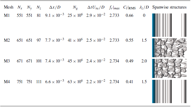
). A mesh independence study is shown in table 1 using four such meshes, referred to as M1, M2, M3 and M4. All these mesh configurations are used to calculate a particular flow case, case I, from table 2 that lies in the parametric space for mode Y (see also figure 2). All the cases are run for a non-dimensional simulation time of
 $t_{s}U_{\infty }/D\approx 200$
. Because of the higher forcing frequencies, a grid independence study for mode Y is expected to serve as a benchmark for all cases of table 2. The total number of points in
 $N_x$
and
 $N_y$
is varied in a similar fashion while the dominant frequency observed in the SPOD spectra,
 $f_r|_{\textit {max}}$
, the root-mean-square (r.m.s.) of the lift coefficient
 $C_l|_{\textit {RMS}}$
and the spanwise wavelength of the vortical structures
 $\lambda _z/D$
are tracked and reported in table 1. There are some differences in the r.m.s. lift coefficient for different mesh resolutions (
 $\Delta C_l|_{\mathit{RMS}} \approx 0.1$
), which might arise from errors involved in computing the pressure on the surface of the immersed body. However, the main spatio-temporal features of mode Y, including the frequency and spanwise wavenumber, are captured accurately in meshes M2 and M4, while they fluctuate for intermediate mesh resolutions, including cases not reported here. Thus, mesh M2 with total mesh points
 $N_g = 41 \times 10^6$
is used throughout this study as the spanwise wavelength and the spanwise structures are converged well while the benefits from even finer meshes appear marginal when compared with their very high computational costs.
Different mesh resolutions showing some important numerical and flow parameters. Here,
 $\Delta x/D$
is the streamwise spatial resolution,
 $N_g$
is the mesh size,
 $\Delta t U_{\infty }/D$
is the time resolution and
 $f_r|_{\textit {max}}$
is the frequency ratio at which the maximum energy is observed in the SPOD spectrum (see figure 6
 $a$
). Among flow parameters,
 $C_l|_{\mathrm{RMS}}$
is the r.m.s. value of lift coefficient and
 $\lambda _z/D$
is the spanwise wavelength of the vortical structures, which is visualised in the last column via a
 $Q$
-criterion of
 $Q=0.1$
in the wake.
 $\lambda _z/D$
reported here are averaged values calculated over the domain
 $x/D\in [0.5,3]$
and
 $y/D\in [0.5,1.5]$
.

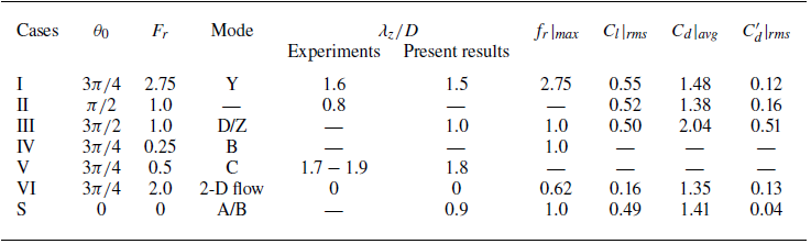
Summary of cases simulated in this study, their flow parameters and the observed modal structure (see also figure 2). Case II did not yield the ‘mode Z’ of the experiments while case S indicates the stationary cylinder case, used here as a reference. The spanwise wavelengths
 $\lambda _z/D$
of the present results are matched with the experiments of Bhattacharyya et al. (Reference Bhattacharyya, Khan, Verma, Kumar and Poddar2022) whenever possible, while the lift and drag coefficients are recorded for some. Case IV results for
 $\lambda _z/D$
are not reported for its poor spanwise coherence.
 $f_r|_{\textit {max}}$
records the dominant frequency from SPOD results for selected cases.

2.2. Spectral proper orthogonal decomposition
Quite a few techniques are now available to extract coherent structures from a turbulent flow field, but arguably the most prevalent is the proper orthogonal technique (POD), originally due to Lumley (Reference Mittal and Kumar1967). A frequency domain version of POD, recently popularised by Towne, Schmidt & Colonius (Reference Unal and Rockwell2018), called the SPOD, is used in this study. It extracts spatio-temporally orthogonal modes ranked by their modal energy, and if the flow is statistically stationary, these modes together would optimally represent the coherent spatio-temporal features of the azimuthally oscillating cylinder wake flow. Although the spatial form of the POD has been used in the past to analyse coherent structures in two-dimensional azimuthally oscillating cylinder flows (e.g. Bhumkar & Sengupta Reference Bhumkar and Sengupta2009), such modes are transparent to the temporal correlations of the underlying turbulent data and thus, the resulting coherent structures are not usually temporally coherent or monochromatic. Dynamic mode decomposition (DMD) is another approach that has also been recently used for transversely oscillating cylinders to decouple the oscillation modes from the Kármán vortex street modes (see Ping et al. Reference Poncet2021). The SPOD modes used here, in fact, represent an ensemble of optimally averaged DMD modes (see Towne et al. Reference Unal and Rockwell2018) which can thus reduce the noise in DMD modes in addition to ranking the modes based on their energy content.
The SPOD approach employs an eigenvalue decomposition of the cross-spectral-density tensor,
 $\boldsymbol{C}$
, to obtain the SPOD modes,
 $\boldsymbol{\psi }$
which are monochromatic, given by
 \begin{equation} \int _\varOmega \boldsymbol{C}(\boldsymbol{x}_1,\boldsymbol{x}_2,f_r)\boldsymbol{\psi }(\boldsymbol{x}_2, f_r)\mathrm{d}\boldsymbol{x}_2 = \lambda (f_r)\boldsymbol{\psi }(\boldsymbol{x}_1,f_r), \end{equation}
where
 $\varOmega$
represents the spatial domain,
 $\boldsymbol{x}_1$
and
 $\boldsymbol{x}_2$
are any two points belonging to
 $\varOmega$
and the eigenvalues,
 $\lambda (f_r)$
, represent the energy associated with the SPOD mode
 $\boldsymbol{\psi }(\boldsymbol{x},f_r)$
. To compute the SPOD modes numerically, we use the open-source code due to Towne et al. (Reference Unal and Rockwell2018). Since the coherent features of the flow are restricted to the wake region, we choose the domain,
 $\varOmega$
, for the SPOD to be the cuboid,
 $x\in [-5D,30D ], y\in [-5D,5D ], z\in [-4.5D,4.5D ]$
and use the velocity field data
 $\boldsymbol{u}/U_{\infty }$
on the mesh in this restricted domain to compute the cross-spectral-density matrix. To do so, ‘snapshots’ of the spatial flow field are obtained at time intervals of
 $\Delta T = 0.1$
(i.e. at a sampling frequency of
 $10$
) and the Welch method is adopted to estimate the power spectral density (PSD). In this study, a total of
 $N_t = 4000$
snapshots are collected while the Fourier transform of these spatio-temporal data is computed by dividing it into blocks of duration
 $T_B = 40$
, i.e. ensembles of size
 $N_e = 400$
(a spectral resolution of
 $\Delta f / f_0 = 0.125$
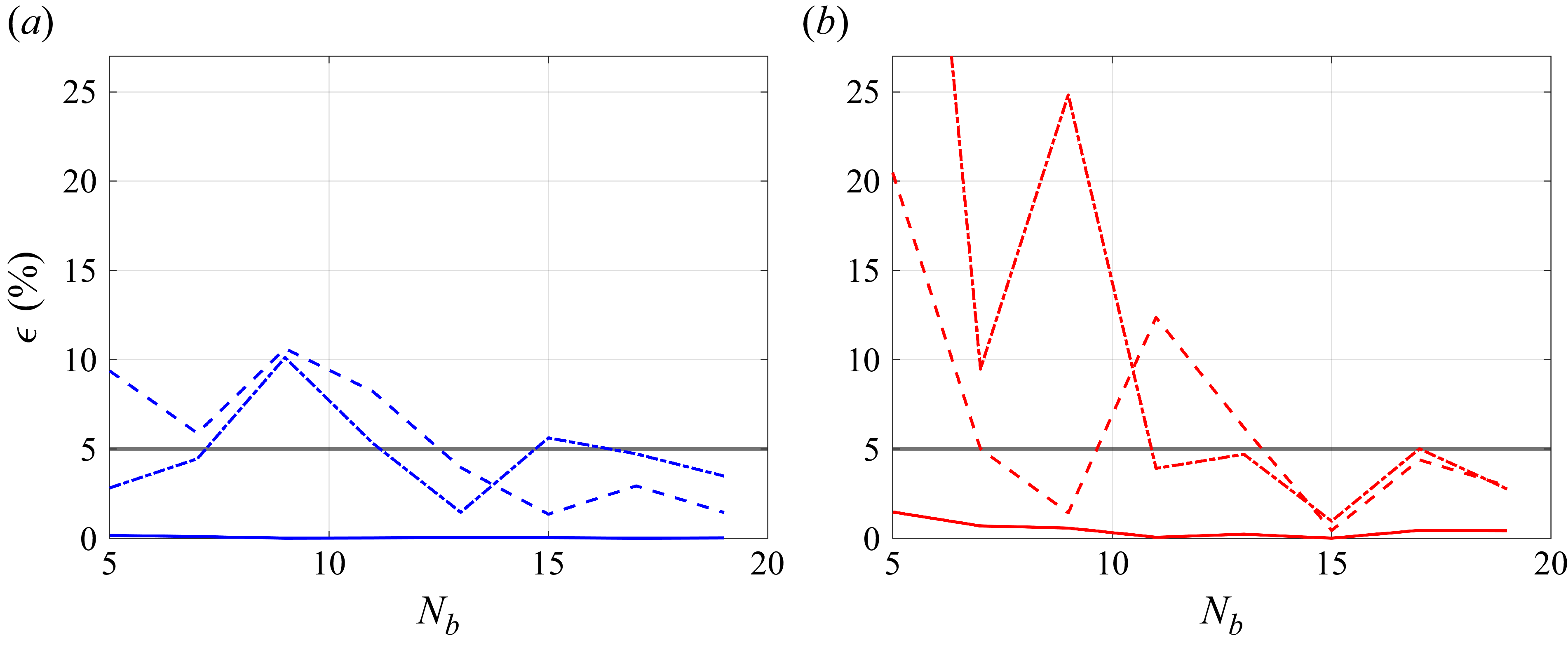
) with a 50 % temporal overlap. A Hamming window function is employed to reduce spectral leakage. The procedure thus yielded
 $N_b = 19$
ensembles. The SPOD analysis shows the energy (i.e.
 $|\lambda (f_r)|$
) to be concentrated in the first few dominant modes, while that for other modes the energy is found to be relatively insignificant for the cases studied here. A convergence study of the SPOD modes so calculated is discussed in Appendix A.2.
3. Results and discussion
In this section, we first discuss the results from the range of the azimuthal amplitude of oscillation
 $\theta _0$
and the frequency ratio
 $F_r$
over which computations were performed in this study. Since the experiments of Bhattacharyya et al. (Reference Bhattacharyya, Khan, Verma, Kumar and Poddar2022) have directly motivated our study, the first objective here is to identify via DNSs the different modal structures they reported, including their novel three-dimensional modes Y and D/Z. As in the experiments, these different modal regimes are first identified by noting the nature of the spanwise structures and their corresponding spanwise wavelengths. Figure 2 shows this parametric space, where, along with the cases investigated in this study, we mark the cases reported in Bhattacharyya et al. (Reference Bhattacharyya, Khan, Verma, Kumar and Poddar2022). The figure also indicates the basic nature of spanwise structures of these modes, visualised using the
 $Q$
-criterion (isosurface based on the second invariant of the velocity gradient tensor), for easy reference throughout this work. The current numerical cases are further summarised in table 2. In what follows in this section, § 3.1 discusses the identification of the three-dimensional modes Y and D/Z, while the other modes are briefly summarised in Appendix A.1. Section 3.2 describes an SPOD of these modes to investigate their spatio-temporal character in detail. This is followed by § 3.2.2, which examines whether these modes are stable configurations on their own or if these are minor variations to other flow configurations that are located nearby (e.g. the two-dimensional flow mode) in the parametric space (see figure 2). Finally, the effect of these modes on the lift and drag forces is discussed in§ 3.2.3, by focusing on their respective phase-averaged vortex-shedding sequence.
3.1. Identification and validation of the three-dimensional modes
3.1.1. Mode Y
Among the three-dimensional modes reported in Bhattacharyya et al. (Reference Bhattacharyya, Khan, Verma, Kumar and Poddar2022), mode Y is characterised by cellular or honeycomb-like spanwise vortex structures in the near wake with a strong spatial coherence up to a streamwise distance of
 $4D$
from the cylinder. This particular three-dimensional mode spontaneously arises within a rather narrow parametric range, which is completely surrounded by two-dimensional wake flow structures (see the shaded region in figure 2). In figure 3, a visual comparison between the current results and the experiments of Bhattacharyya et al. (Reference Bhattacharyya, Khan, Verma, Kumar and Poddar2022) is shown for case I (i.e.
 $\theta _0 = 3\pi /4$
and
 $F_r = 2.75$
, see also table 2). Figures 3(a) and 3(c) are based on the instantaneous spanwise vorticity magnitude and the
 $Q$
-criterion from the current DNS, respectively, while figures 3(b) and 3(d) are the hydrogen bubble flow visualisation images from Bhattacharyya et al. (Reference Bhattacharyya, Khan, Verma, Kumar and Poddar2022). The qualitative similarity between the two sets of images is striking, with the vortex core locations in the
 $x{-}y$
plane in figure 3
 $(a)$
matching with the experimental visualisations of figure 3
 $(b)$
. This array of counter-rotating vortices seems to be coherent up to
 $x \sim 4D$
, similar to the observations in the experiments, beyond which the cells become flatter and the far wake essentially becomes chaotic. The spanwise view shown in figure 3
 $(c)$
(present study) and figure 3
 $(d)$
(experiments) highlights the typical honeycomb pattern of this mode.
Visualisations of mode Y corresponding to case I (
 $\theta _0 = 3\pi /4$
and
 $F_r =2.75$
, see table 2), showing
 $(a)$
vorticity contours (
 $|\omega _z|$
) at
 $z/D=3$
and
 $(c)$
spanwise vortices visualised via the
 $Q$
-criterion (
 $Q=0.1$
) based on present simulations, compared with
 $(b)$
top and
 $(d)$
side views of the corresponding experimental images, respectively (Bhattacharyya et al. Reference Bhattacharyya, Khan, Verma, Kumar and Poddar2022). Additionally,
 $(e)$
shows
 $w/U_{\infty }$
variation at
 $(x,y)$
=
 $(1.6D,0.5D)$
(marked as a vertical dashed line in
 $c$
) and
 $(f)$
shows the PSD of the same, where the dominant wavelength is highlighted via a vertical dashed line.

A quantitative comparison between the experiments and simulations can be made by examining the spanwise wavelength,
 $\lambda _z/D$
, of these vortical structures. In the experiments, the wavelength was estimated directly from the digital images by extracting the pixel intensity profile along a line across the dominant spanwise structures and using a Fourier transform. In this study, this is achieved by considering the instantaneous
 $w$
-velocity profile in the
 $x$
-
 $z$
plane, which, likewise in the experiments, is measured along a straight line located at
 $x/D = 1.6$
and
 $y/D = 0.5$
(see figure 3
 $c$
) to obtain a profile as shown in figure 3
 $(e)$
. A Fourier transform of this signal yields the spanwise wavelength of the spatial structures as
 $\lambda _z/D \sim 1.5$
, which compares well with the experimentally reported value of 1.6 (see table 2). Although the experiments did not report the downstream location at which this wavelength was calculated, our simulated mode Y is seen to possess very good spatial coherence so that the calculated
 $\lambda _z/D$
is insensitive to the downstream location if
 $x/D \leq 4$
.
Visualisations of case II of table 2 (
 $\theta _0 = \pi /2$
and
 $F_r = 1$
), showing
 $(a)$
contours of
 $|\omega _z|$
at
 $z/D=0$
and
 $(b)$
spanwise vortices visualised via the
 $Q$
-criterion (
 $Q=0.1$
) based on the present simulations, the latter compared with
 $(c)$
spanwise view of corresponding experimental images (Bhattacharyya et al. Reference Bhattacharyya, Khan, Verma, Kumar and Poddar2022).

An interesting aspect of mode Y seems to be its rather sudden appearance in the mode map of figure 2. This has been discussed in Bhattacharyya et al. (Reference Bhattacharyya, Khan, Verma, Kumar and Poddar2022), where they were able to distinguish this mode, first at
 $\theta _0 = 135^{\circ }$
with
 $2.4 \lt F_r \lt 2.8$
and then again with the forcing ratio
 $F_r$
fixed at
 $2.75$
and
 $123^{\circ } \lt \theta _0 \lt 138^{\circ }$
. These experimental data points are marked in figure 2. In this study, an attempt is made to better trace the boundary of this mode on the parametric space by observing the clarity of the spanwise structures and their expected wavelength. This is shown as the shaded area in figure 2, which is also seen to approximately include the experimental data points. Of course, the present computations have extended the existence of mode Y to higher forcing frequencies (
 $F_r \approx 3.25$
) than was possible in the experiments. Further, with increased forcing, the mode gets confined over an increasingly narrow band of
 $\theta _0$
. Outside the shaded region, the wake remains two-dimensional. The relation between mode Y and the surrounding two-dimensional flow is further analysed in § 3.2.2. Although computations at other Reynolds numbers is not an objective of the present work, preliminary results of mode Y with the same parameters of case I but at higher
 ${\textit{Re}}$
indicate the presence of similar honeycomb-like structures even at
 ${\textit{Re}} = 500$
, but with a reduced spanwise spacing.
3.1.2. Mode D/Z
The other three-dimensional mode D/Z reported in Bhattacharyya et al. (Reference Bhattacharyya, Khan, Verma, Kumar and Poddar2022) appeared when the forcing frequency matched the shedding frequency of the stationary cylinder, i.e. when
 $F_r \approx 1$
. Although it seems to have been observed over a rather narrow band of
 $0.9 \lt F_r \lt 1.1$
, mode D/Z was most clear at
 $F_r = 1$
. On the other hand, keeping
 $F_r = 1$
fixed, mode D/Z appeared over a wide range of azimuthal amplitudes:
 $80^{\circ } \lt \theta _0 \lt 180^{\circ }$
. An attempt was made to numerically capture mode D/Z at the parameters of case II (
 $\theta _0 = \pi /2$
and
 $F_r = 1$
), where it was originally observed in the experiments. The results are compared in figure 4, where the spanwise variations seen in experiments in figure 4
 $(c)$
are missing in the simulations in figure 4
 $(b)$
, where the wake flow remains two-dimensional. This is not an artefact of the finite cylinder span as even on repeating the case II simulations with longer cylinder spans of
 $L_z = 18D$
and
 $27D$
, it still did not yield any spanwise three-dimensionalities. We note that although the three-dimensional characteristics are not observed here, the vortex cores shown in figure 4
 $(a)$
align well with experiments (figure 5
 $b$
).
Now, at
 $F_r = 1$
, both a Floquet stability analysis (see Lo Jacono et al. Reference Lo Jacono, Leontini, Thompson and Sheridan2010) and numerical computations (see Poncet Reference Pralits, Brandt and Giannetti2004) have reported the existence of three-dimensionalities only close to the cylinder. In fact, Poncet (Reference Pralits, Brandt and Giannetti2004) also reported three-dimensionalities to disappear at the parameters of case II, as seen here, although at a higher
 ${\textit{Re}}=400$
. Further, if
 $\theta _0$
is increased, the vortex columns become more compact and shift closer to the oscillating cylinder (Lo Jacono et al. Reference Lo Jacono, Leontini, Thompson and Sheridan2010), which can in turn yield three-dimensional mode D/Z structures that are now placed nearer to the cylinder and are perhaps less diffused (see Bhattacharyya et al. Reference Bhattacharyya, Khan, Verma, Kumar and Poddar2022). To verify this, a higher amplitude situation, case III (
 $\theta _0 = 3\pi /2$
and
 $F_r = 1$
, see table 2) is simulated, results of which are shown in figure 5. For comparison, visualisations from Bhattacharyya et al. (Reference Bhattacharyya, Khan, Verma, Kumar and Poddar2022) for case II are also included. The spanwise view of these vortices in figure 5
 $(c)$
now clearly shows the presence of a mode D/Z instability. Curiously, the
 $\theta _0$
when scaled by
 $2\pi$
, yields an amplitude of
 $0.75$
, which lies inside the parameter space where Lo Jacono et al. Reference Lo Jacono, Leontini, Thompson and Sheridan2010) reported the existence of their mode D (at
 $\theta _0 \gt 1.3\pi$
), visually identical to the present mode D/Z, being of the same double row vortex-shedding structure. In Bhattacharyya et al. (Reference Bhattacharyya, Khan, Verma, Kumar and Poddar2022), mode D/Z is attributed to the braid shear layer instabilities between the first and second shed vortices, so that it primarily grows between the second and third wake vortices. The present computations seem to indicate this (see figure 5
 $c$
) with the instabilities mostly disappearing beyond
 $x/D \gt 4$
, although the spanwise sinuous oscillation of the vortex core persists (see figure 5
 $c$
).
Visualisations of mode corresponding to case III (
 $\theta _0 = 3\pi /2$
and
 $F_r = 1$
, see table 2), showing
 $(a)$
contours of
 $|\omega _z|$
at
 $z/D=0$
and
 $(c)$
spanwise vortices visualised via the
 $Q$
-criterion (
 $Q=0.1$
) based on the present simulations, compared with
 $(b)$
top and
 $(d)$
side views of corresponding experimental images for case II (
 $\theta _0 = \pi /2$
and
 $F_r = 1$
), respectively (Bhattacharyya et al. Reference Bhattacharyya, Khan, Verma, Kumar and Poddar2022). Additionally,
 $(e)$
shows
 $w/U_{\infty }$
variation at
 $(x,y)$
=
 $(2D,-0.7D)$
(marked as vertical dashed line in
 $c$
) and
 $(f)$
shows the PSD of the same, with the dominant wavelength highlighted via a vertical dashed line.

Similar to the mode Y above, the spanwise periodicity for mode D/Z is measured by calculating the instantaneous
 $w$
-velocity profile along the straight line located at
 $x/D = 1$
and
 $y/D = 1$
(see figure 5
 $c$
), and plotted in figure 5
 $(e)$
. The Fourier transform yields a dominant spanwise wavelength of
 $\lambda _z/D \sim 1$
here (see figure 5
 $f$
), which is also tabulated in table 2. Compared with the
 $\lambda _z/D \approx 0.8$
of case II, as obtained in the experiments, our numerically computed value is higher (
 $\lambda _z/D = 1$
), which might be due to the differences in
 $\theta _0$
and the variations in the streamwise spacing between vortices. Although, the Floquet analysis of Lo Jacono et al. (Reference Lo Jacono, Leontini, Thompson and Sheridan2010), yielded a spanwise wavelength of
 $\lambda _z\approx 0.9$
which matches better with the computed value for case III, further confirming the apparent similarity between the modes Z and D, although the latter was obtained at a slightly different
 ${\textit{Re}}=300$
. At
 ${\textit{Re}}=500$
, for example, the characteristic spanwise vortex core oscillations of mode D/Z is not observed for the parameters of case III (not shown here). In figure 5
 $(f$
), a subharmonic peak at
 $\lambda _z/D = 0.5$
is also seen, suggesting that nonlinear interactions are appreciable under these conditions. Nevertheless, it must be noted that the spanwise oscillation amplitudes here are relatively low compared with mode Y.
Coherent spatio-temporal features for case I of table 2 (mode Y), showing
 $(a)$
the first SPOD eigenvalue (
 $|\lambda ^{(1)}(f_r)|$
) (black curve) and power spectrum of fluctuating spanwise velocity from a probe at
 $(x,y,z) = (D,0.5D,0)$
(grey curve) as a function of
 $f_r$
, while the contours of
 $w/U_\infty$
are shown for
 $(b,h)$
DNS results and the corresponding five leading SPOD eigenmodes at
 $(c,i)$
 $f_r = 0.62$
;
 $(d,j)$
 $f_r = 1.37$
;
 $(e,k)$
 $f_r = 2.75$
;
 $(f,l)$
 $f_r = 4.12$
; and
 $(g,m)$
 $f_r = 5.37$
, all shown as projections on the
 $z$
(left) and
 $y$
-planes (right), respectively. The horizontal line in any view traces the location of the viewing plane for the other view.

Contours of streamwise vorticity
 $\omega _x$
for the dominant SPOD mode, occurring at
 $f_r=2.75$
for case I, shown on (a)
 $y{-}z$
plane at
 $x/D=2$
and (b)
 $x{-}z$
plane at
 $y/D=0.5$
.

3.2. Dynamics of the three-dimensional modes
After numerically confirming the presence of the three-dimensional modes Y and D/Z in the wake of an azimuthally oscillating cylinder at
 ${\textit{Re}}=250$
, the present section focuses on their dynamics. In the experiments of Bhattacharyya et al. (Reference Bhattacharyya, Khan, Verma, Kumar and Poddar2022), limited investigations on the modal dynamics were attempted. Primary among them was the use of hot-wire measurements to analyse the spectral content of the wake along the spanwise direction at conditions when these modes were seen. For case II of table 2, these measurements confirmed a perfect lock-on phenomenon as there was always a strong peak at
 $f_r = 1$
for all the spanwise locations measured. On the other hand, for the Y mode (case I of table 2), these measurements indicated that there were more frequencies present in the wake beyond the forcing frequency of
 $2.75$
, thus suggesting a more complex character. In § 3.2.1, we perform a detailed spatio-temporal analysis of these modal structures via the SPOD technique discussed in § 2.2. Later, in § 3.2.2, we focus on how the Y and D/Z modes are dynamically connected to the two-dimensional modes by performing a correlation analysis. Finally, in § 3.2.3 we comment on how the measured lift and drag forces are altered with the onset of three-dimensionalities in the modes, which are expected to be important in practical applications.
3.2.1. Spatio-temporal characteristics
The SPOD results for case I, for which mode Y is observed (
 $\theta _0 = 3\pi /4$
and
 $F_r = 2.75$
, see table 2), are shown in figure 6. These computations follow the procedures described in § 2.2, with
 $\lambda (f_r)$
being the eigenvalue corresponding to the SPOD eigenmode
 $\boldsymbol{\psi }(\boldsymbol{x},f_r)$
. Figure 6
 $(a)$
shows the energy spectra of the most dominant SPOD mode
 $\lambda ^{(1)}(f_r)$
as a function of
 $f_r$
. Here, the frequency axis is limited to
 $0.1\le f_r\le 10$
to focus on the region containing maximum energy in the spectra (our full data have
 $f_r$
up to
 $25$
). Several spectral peaks are observed at specific
 $f_r$
values whose existence is qualitatively indicated in the study of Bhattacharyya et al. (Reference Bhattacharyya, Khan, Verma, Kumar and Poddar2022). The power spectrum of the fluctuating spanwise velocity measured using a probe at
 $(x/D,y/D,z/D) = (1, 0.5, 0)$
in the simulations is plotted alongside the SPOD spectrum for comparison, highlighting the similarities between the two.
We analyse the first five spectral peaks of the dominant SPOD mode in figures 6(c–g) and 6(i–m). Spectral peaks beyond the first five have energy content that is almost two orders of magnitude below the most dominant peak and are therefore not considered to be dynamically significant. For comparison, figures 6(b) and 6(h) show the instantaneous
 $w$
-velocity contours from the DNS at an arbitrary time. The SPOD modes are visualised at an arbitrary phase and, for clarity, as projections on the ‘top view’
 $z$
-plane at
 $z/D = 0$
(see figure 6
 $b{-}g$
) and the ‘span view’
 $y$
-plane at
 $y/D = 0.5$
(see figure 6
 $h{-}m$
). For reference, each of these planes is also marked as horizontal lines in the corresponding orthogonal plane in figure 6
 $(b{-}m)$
. The first five spectral peaks for case I are observed at
 $f_r = 0.62, 1.37, 2.75, 4.12$
and
 $5.37$
, as also marked in figure 6 against the appropriate rows of figures. The forcing frequency for this case is at
 $F_r=2.75$
, which naturally appears in figure 6
 $(a)$
as the spectral peak
 $f_r=2.75$
with the highest energy content. The lowest-frequency peak at
 $f_r = 0.62$
and shown in figures 6(c) and 6(i) appears to correspond to the far wake of the flow field (compare with figures 6(b) and 6(h), respectively). This particular spectral peak, solely defining the dynamics of the far wake, is not detected by the probes, which are placed close to the oscillating cylinder inside the near wake. The
 $y$
-plane
 $w$
-velocity DNS contours (see figure 6
 $h$
) clearly show the previously observed spanwise periodicity corresponding to the Y modes at
 $\lambda _z/D \sim 1.5$
(see table 2). Interestingly, this wavelength is not observed at the frequency of
 $f_r = 2.75$
(see figure 6
 $k$
) but instead at the corresponding subharmonic of the forcing frequency of
 $2.75$
at
 $f_r = 1.37$
(see figure 6
 $j$
) which also has comparable energy content as seen in figure 6
 $(a)$
. This suggests that the distinctive mode Y structures actually occur as a subharmonic of the forcing frequency. The subharmonic and the forcing frequency are, therefore, the two most important frequencies for this mode. Further, as can be observed from figure 6
 $(k)$
, at the frequency of
 $f_r=2.75$
, the spanwise periodicity is almost double that of mode Y. The same has been verified (not shown here) via a phase averaging of the DNS data at the given forcing frequency. This increased the periodicity of the spanwise structures in mode Y to twice that in DNSs and identical to what is observed with the corresponding SPOD mode at
 $f_r = 2.75$
. While the results are not unexpected, as SPOD structures are indeed phase-correlated organised structures, physically, it also indicates that the cells that originate on the cylinder surface switch their spanwise location during each cycle of cylinder oscillation (see supplementary movie 3). Figure 7 shows the streamwise vorticity contours corresponding to the most dominant SPOD mode (
 $f_r=2.75$
) on the two perpendicular planes containing the cylinder span. Clearly, the vorticity structures resemble the honeycomb-like patterns observed for the
 $w$
-velocity contours. In figure 6, all the spectral peaks starting from the second peak at
 $f_r=1.37$
correspond to spatio-temporal events at the near wake, next to the cylinder. At higher frequencies, the streamwise wavelengths reduce (i.e. along
 $x/D$
) and so does their spatial support (see figures 6
 $(f,l)$
and 6
 $(g,m)$
). Nevertheless, these higher spectral peaks occur approximately at the harmonics of the forcing frequency (at
 $f_r = 5.37$
) and its subharmonic (at
 $f_r = 4.12$
), giving further credence to the importance of frequencies
 $f_r = 1.37$
and
 $2.75$
toward the dynamics of mode Y of case I.
Coherent spatio-temporal features for case III of table 2 (mode D/Z) showing
 $(a)$
the first SPOD eigenvalue (
 $|\lambda ^{(1)}(f_r)|$
) (black curve) and power spectrum of fluctuating spanwise velocity from a probe at
 $(x,y,z) = (D,0.5D,0)$
(grey lines) as a function of
 $f_r$
, while the contours of
 $w/U_\infty$
are shown for
 $(b,h)$
DNS results and the corresponding five leading SPOD eigenmodes at
 $(c,i)$
 $f_r = 0.5$
;
 $(d,j)$
 $f_r = 1.0$
;
 $(e,k)$
 $f_r = 1.5$
;
 $(f,l)$
 $f_r = 2.0$
; and
 $(g,m)$
 $f_r = 3.0$
, all shown as projections on the
 $z$
(left) and
 $y$
-planes (right), respectively. The horizontal line in any view traces the location of the viewing plane for the other view.

Contours of streamwise vorticity
 $\omega _x$
for the dominant SPOD mode, occurring at
 $f_r=1.0$
for case III, shown on (a)
 $y{-}z$
plane at
 $x/D=2$
and (b)
 $x{-}z$
plane at
 $y/D=0.5$
.

Cross-correlation between cases I (mode Y) and III (mode D/Z) with case VI (forced two-dimensional flow) of table 2 are shown in
 $(a)$
as a split graph for the respective correlation contours. The red star in
 $(a)$
indicates
 $f_r = 0.5$
for which isosurfaces of Q at
 $5 \times 10^{-5}$
are shown for
 $(b)$
case III (mode D/Z);
 $(c)$
case VI (forced two-dimensional flow) and
 $(d)$
case I (mode Y) to demonstrate any visual similarity between them, if at all. The blue dashed lines in
 $(a)$
show the dominant frequencies of the SPOD spectra for these modes (see figures 6, 8 and 15), respectively.

Next, we focus on the most dominant SPOD mode for mode D/Z, which is extracted from case III of table 2. Like mode Y before, the corresponding modal pictures for mode D/Z are shown in figure 8. Here, the first five spectral peaks are identified at
 $f_r = 0.5, 1, 1.5, 2$
and
 $3$
, whose mode shapes are shown in figures 8
 $(c{-}g)$
and 8
 $(i-m)$
, for projections on the
 $z$
-plane and
 $y$
-plane, respectively. Similar to mode Y, the first spectral peak at the subharmonic of the forcing frequency at
 $f_r = 0.5$
is not detected by the probes, indicating its presence in the far wake. This is confirmed from figures 8(c) and 8(i) where this frequency appears to have significant spatial support only at the far downstream
 $x/D \gt 10$
. These far-wake features are also observed at all higher harmonics of this frequency, especially for
 $x/D \geq 20$
, albeit with decreasing streamwise wavelengths and reduced coherence. At the frequency of
 $f_r = 1$
, in addition to these far wake features, the SPOD mode corresponding to the forcing frequency also shows strong three-dimensional coherence in the near wake (see figures 8
d and 8
j). This is distinct from what is observed for mode Y, where the far wake seems to oscillate at a unique frequency (e.g.
 $f_r = 0.62$
for case I, see figure 6) while the near-wake fluctuations are composed of the forcing frequency, its subharmonic and harmonics. In contrast, for the mode D/Z here, the SPOD mode corresponding to the oscillating cylinder forcing frequency
 $f_r=1$
and its harmonics
 $f_r=2,3$
(see figures 8
j, 8
l and 8
 $m$
, respectively) shows the spanwise structures at
 $\lambda _z/D \sim 1$
, as observed in the DNS (see figure 8
 $h$
), thus largely defining the nature of mode D/Z. The streamwise vorticity contours at the dominant frequency (
 $f_r=1$
) are plotted in figure 9, which expectedly show the rib-like patterns observed in the corresponding DNS results (see figure 8
 $h$
).
3.2.2. Connection with other modes
The modal map of the oscillating cylinder plotted in figure 2 shows a region in the parametric space of a forced two-dimensional (2-D) flow state (case VI,
 $\theta _0 = 3\pi /4$
and
 $F_r = 2$
, see table 2 and figure 14 in Appendix A) in between the parameter spaces of the numerically obtained mode D/Z (case III,
 $\theta _0 = 3\pi /2$
and
 $F_r = 1$
) and mode Y (case I,
 $\theta _0 = 3\pi /4$
and
 $F_r = 2.75$
), respectively. Here, we investigate the connections between these newly discovered 3-D modes with this forced 2-D flow state using SPOD and correlation analysis. Other modes do not show significant correlations which are not reported here. For this purpose, the magnitude of the Pearson correlation coefficient,
 $R_{1,2}$
, between two SPOD modes
 $\boldsymbol{\psi _1}$
and
 $\boldsymbol{\psi _2}$
for a pair of frequencies
 $(f1, f2)$
is calculated via
 \begin{equation} R_{1,2}(f_1,f_2)=\frac {|{\boldsymbol{\psi _1}^{\ast }}(\boldsymbol{x},f_1)\boldsymbol{\psi _2}(\boldsymbol{x},f_2)|}{{|\boldsymbol{\psi _1}(\boldsymbol{x},f_1)||\boldsymbol{\psi _2}(\boldsymbol{x},f_2)|}}, \end{equation}
where
 $(\;)^\ast$
represents the conjugate transpose and
 $|\ast |$
represents the magnitude. Here, the full 3-D, complex, SPOD mode
 $\boldsymbol{\psi }(\boldsymbol{x},f_r)$
, as discussed in § 2.2, is used for the calculation of
 $R_{1,2}$
at any pair of frequencies
 $(f1,f2)$
, with them restricted between
 $0 \lt f_r \lt 5$
. Figure 10
 $(a)$
shows the contours for
 $R_{1,2}$
between both the modes Y and D/Z with the forced 2-D flow, superimposed into the same plot separated via a diagonal line, with the left and right halves corresponding to correlations between the cases of forced 2-D flow with modes Y and D/Z, respectively. The dotted lines in the plot represent the frequency at which peaks occur in the SPOD spectra for the corresponding modes with the horizontal lines corresponding to the peaks of the modes Y and D/Z (see figures 6(
 $a$
) and 8(
 $a$
), respectively), while the vertical lines show the SPOD peaks of the forced 2-D flow (see figure 15 of Appendix A). These lines serve as a useful guide in the frequency parametric space where cross-correlations are expected to have significant magnitude (
 $R_{1,2} \gtrsim 0.7$
), if there are similarities in coherent features. From the figure 10
 $(a)$
, it can be observed that both the 3-D modes are significantly correlated with the forced 2-D mode at the lower forcing frequencies, especially at
 $f_r \lt 1$
. Such strong cross-correlations are not unexpected since the vortex structures at the lower
 $f_r$
are the natural 2-D vortex-shedding modes, common for all the non-lock-on regions in figure 2 and irrespective of the nature of forcing. This can be inferred by comparing figures 6
 $(c,i)$
and 8
 $(c,i)$
for modes Y and D/Z, respectively, where the SPOD modes have strong energy content in the far wake for both modes. Mode Y shows a maximum correlation of
 $R_{1,2}=0.74$
with the 2-D flow case (at
 $f_r=0.625$
for both the 2-D flow and mode Y), while mode D/Z is higher, with
 $R_{1,2} = 0.92$
(at
 $f_r=0.625$
of 2-D flow and
 $f_r=0.5$
of mode D/Z). The higher correlations between mode D/Z and the 2-D flow are surprising considering that these two are farther apart in the parameter space (cases III and VI in table 2, see also figure 2) than mode Y. For a visual comparison, figures 10(b), 10(c) and 10(d) show the vortical structures from the cases III, VI and I of table 2, respectively, at the frequency of
 $f_r=0.5$
(also marked by a red in figure 10
 $a$
), since the maximum correlations between the 3-D modes with the 2-D flow is observed near this frequency. The vortex contours in these figures are derived from the
 $Q$
isosurfaces for the three cases which are extracted from the real part of the SPOD mode
 $\boldsymbol{\psi }(\boldsymbol{x},f_r)$
, consisting of the velocity components
 $(u, v, w)$
. As can be observed by comparing figures 10(b) and 10(c), the vortex core locations for the modes D/Z and the 2-D flow are strikingly similar, except that, for mode D/Z, some spanwise vortical perturbations in the vortex cores are also visible. Such visual similarity, coupled with the high cross-correlation values of mode D/Z (see figure 10
 $a$
) with forced 2-D flow and its saturated nature, suggests that mode D/Z is unlikely to be a new mode. This is also corroborated by the high correlations that exist near
 $f_r = 1$
. Thus, mode D/Z might likely be a consequence of the oscillation amplitude matching the vortex shedding, leading to a resonance phenomenon with the so-called mode D/Z representing an intermediate state as the 3-D mode B transitions to the forced 2-D flow mode.
The mode Y case also consists of vortex cores at the far wake (e.g. figure 3
 $c$
), located similarly to the other two cases, but is also superimposed by strong 3-D structures. Thus, the correlations are lower and negligible, especially at the frequencies corresponding to the forcing frequency,
 $f_r=2.75$
and its harmonics (see figure 10
 $a$
). Hence, compared with the forced 2-D flow, mode Y appears to be a 3-D mode with unique hydrodynamic signatures, very different from the former, even though it is in closer proximity to the 2-D flow in the parameter space. Further, note that, in figures 10(b), 10(c) and 10(d), vortex cores can be seen to gradually grow in size downstream due to the phenomenon of vortex merging. Here, smaller vortices in the near wake eventually combine to form large-scale vortices at the far wake, as a consequence of vortex synchronisations due to cylinder oscillations at the higher forcing frequencies of these cases. The same merging phenomenon is also visible in the instantaneous pictures of figures 6 and 8. Such a vortex merging phenomenon is not observed for the lower
 $F_r$
cases of table 2: cases IV and V (modes B and C, respectively, not shown here).
Variation of
 $(a)$
lift coefficient
 $C_l$
and
 $(b)$
drag coefficient
 $C_d$
over two oscillation cycles shown for
 (black), case I (mode Y);
 (magenta), case II;
 (blue), case III (mode D/Z);
 (red), case VI (forced 2-D flow) and
 (grey), case S (stationary cylinder) of table 2. The
 $\omega _z$
contours are shown for
 $(c)$
case III (mode D/Z);
 $(d)$
case II;
 $(e)$
case VI (forced 2-D flow);
 $(f)$
case I (mode Y) and
 $(g)$
case S (stationary cylinder). In
 $(c-g)$
solid and dashed arrows locate primary and secondary vortices, respectively.

3.2.3. Effects on lift and drag
One of the reasons for imparting azimuthal motions to a stationary cylinder is to modify the wake to remain two-dimensional, which in turn reduces the drag on the body. For example, Poncet (Reference Pralits, Brandt and Giannetti2004) reported a 12 % drop in the drag coefficient for the forced 2-D case when compared with a 3-D flow. The 3-D modes discovered by Bhattacharyya et al. (Reference Bhattacharyya, Khan, Verma, Kumar and Poddar2022) are thus expected to increase the drag (and lift) over the nearby 2-D modes, e.g. the forced 2-D flow from case VI of table 2. We investigate this in the present section. Note that the lift and drag coefficients calculated in this section are for the entire cylinder span and not at a specific cross-section.
Figures 11(a) and 11(b) compare the coefficients of lift (
 $C_l$
) and drag (
 $C_d$
) for the four different cases discussed in § 3.2.2 (cases I, II, III and VI of table 2) over two full oscillation cycles of the cylinder to account for variations due to subharmonics developed in the wake (see figures 6
a and 8
a). Figures 11(a) and 11(b) indicate no significant differences between the oscillations in time intervals
 $[0,T]$
and
 $[T,2T]$
, which is likely because the span-averaged coefficients remain unaffected by the spanwise translation of the coherent structures occurring between the two time intervals so that we may only focus on the first time interval. In addition, figures 11(a) and 11(b) also contain the variation for the stationary cylinder case (see case S of table 2), which serves as an important benchmark for our analysis in this section.
Figure 11
 $(c{-}g)$
show the phase-averaged spanwise vorticity (
 $\omega _z$
) contours on the
 $z$
-plane at
 $z/D=0$
for these five cases, including the stationary cylinder case S, focusing on the vortex shedding in the near wake of the oscillating cylinder. In each case, vorticity contours are plotted at five phases of the oscillation cycle on a single spanwise plane (
 $z/D = 0$
) in order to understand the vortex-shedding patterns and their corresponding effects on the cylinder lift and drag forces. In these snapshots, the primary and secondary vortex cores, if visible, are located with solid and dashed arrows, respectively, whose data are phase averaged over eight oscillation cycles.
Figure 11
 $(c)$
shows the shedding cycle for case III of table 2. This is the parameter space where mode D/Z is observed in the present computations. Here, a single pair of vortices is shed from the top and bottom surfaces of the cylinder during each oscillation cycle. Interestingly, the time snapshots show the primary shed vortices to have the same positive sense of vorticity at all times, wrapped around by a negative vorticity region. To the best of our knowledge, the occurrence of all primary vortices being composed of a core of one sign, surrounded by an annular region of opposite sign, has not been reported previously. Here, it seems to be due to the high oscillation amplitude (
 $\theta _0 = 3\pi /2$
) of the case, which might induce flow separation, coupled with the effect of the forcing frequency matching the natural shedding frequency (
 $F_r = 1$
). The corresponding
 $C_l$
curve (see the blue dotted curve of figure 11(
 $a$
)) shows multiple peaks, while the
 $C_d$
curve (blue dotted curve of figure 11(b)) follows a sinusoidal pattern with a frequency twice of the forcing frequency, as typically also seen in shedding from stationary cylinders (solid grey curves). The mean drag coefficient,
 $C_d|_{\mathrm{avg}}$
, and the amplitude of its fluctuating component,
 $C_d'$
, for case III are easily the highest (
 $C_{d}|_{\mathrm{avg}}=2.04$
, see table 2) among all the cases studied here, a consequence of the higher forcing amplitude, which causes the shed vortices to be displaced further laterally, yielding a wider wake and larger momentum deficit.
Figure 11
 $(d)$
shows the shedding cycle for case II of table 2. This corresponds to the conditions where ‘mode Z’ was reported by Bhattacharyya et al. (Reference Bhattacharyya, Khan, Verma, Kumar and Poddar2022), but where only a 2-D flow is observed in the current simulations. Similar to case III, a single pair of primary vortices are shed here too (compare with figure 11(c)), with the location of shed vortices being approximately similar (same forcing frequency), but the weaker vortex pairs now have opposite signs of
 $\omega _z$
, similar to the stationary cylinder shedding (see figure 11
g), and are packed much closer together laterally. Of course, the closer lateral spacing is due to the much lower azimuthal oscillation amplitude (
 $\theta _0 = \pi /2$
) in this case. The
 $C_d|_{\mathrm{avg}}$
and
 $C_d'$
values are also lower for case II (see red dash-dotted line in figure 11(b)) when compared with case III (more than
 $32\,\,\%$
lower), although the nature of the oscillation over the full cycle appears to be very similar. The
 $C_l$
variation for this case is similar to case III, except that it follows a smoother sinusoidal pattern without modulations at higher frequencies, again similar to the stationary cylinder case (solid grey curve).
Next, the forced 2-D flow’s (case VI of table 2) shedding pattern is shown in figure 11
 $(e)$
. Here, the appearance of a pair of vortices at the cylinder end with opposite signs immediately resemble case II of figure 11
 $(d)$
when accounting for the higher oscillation frequency (
 $F_r = 2$
), which has just increased the number of vortex cores within the same streamwise spacing, while a slightly higher oscillation amplitude (
 $\theta _0 = 3\pi /4$
) has increased the lateral spread. The same is also reflected in the
 $C_d$
variation over the oscillation cycle (dashed red line), which follows a pattern identical to case II. The
 $C_l$
curve in figure 11
 $(a)$
shows a significant modulation due to its higher shedding frequency (
 $F_r = 2$
), where on each end of the cylinder a shed vorticity region gets entrained by the previous shed vortex (see figure 11
 $e$
).
Figure 11
 $(f)$
shows the shedding cycle for case I of table 2 corresponding to the mode Y. From the shedding patterns, it is clear that case I has a unique shedding cycle where, instead of one, two vortices are shed from either side of the cylinder within an oscillation cycle. Note that these features are also observed in the instantaneous contours of both the present simulations and experiments (see figures 3
 $a$
and 3
 $b$
), implying that these are not due to the phase averaging employed. The spanwise oscillations due to these adjacent vortices, referred to here as the primary and secondary vortex cores, are eventually responsible for the honeycomb-like structure of this mode, as seen in figure 10
 $(d)$
and elsewhere. In spite of such complex shedding patterns, the corresponding
 $C_l$
variation is almost sinusoidal (solid black curve in figure 11(
 $a$
)) with the minor deviation likely from the shedding effects of the weaker secondary vortices. Similar effects are seen with its
 $C_d$
variation in figure 11
 $(b)$
as well.
On comparing the vorticity structures of the stationary cylinder case S (
 $F_r = 0$
), case II (
 $F_r = 1$
), case VI (
 $F_r = 2$
) and case I (
 $F_r = 2.75$
), it is obvious in figure 11
 $(c{-}g)$
that the particular oscillation frequency
 $F_r$
decides the streamwise spacing between the vortices, which has also been observed with 2-D oscillating cylinder simulations (see Choi et al. Reference Choi, Choi and Kang2002). The oscillation amplitude, on the other hand, appears to modify the order of vortices involved in the vortex merging process and hence the wake structure, as seen by comparing case II (
 $\theta _0 = \pi /2$
) and case III (
 $\theta _0 = 3\pi /2$
), which is also seen in 2-D simulations of Choi et al. (Reference Choi, Choi and Kang2002). The latter has a more pronounced effect on the cylinder drag.
On summarising figures 11(a) and 11(b) and table 2, case VI (forced 2-D flow), as expected, has the lowest
 $C_l|_{\mathrm{RMS}}$
and
 $C_d|_{\mathrm{avg}}$
among all the oscillating cases studied here. Case VI has better drag performance even compared with the stationary case (see table 2 and figure 11
 $b$
), however, it is worth noting that cylinder oscillations lead to a higher
 $C_d^{\prime }|_{\mathrm{RMS}}$
than case S, for all the cases studied. This means that, even though specific oscillations may reduce the mean drag value, these also lead to higher drag fluctuations. The only significant flow control advantage observed for case VI is its significant reduction in the lift oscillations, as indicated by its
 $C_l|_{\mathrm{RMS}}$
in figure 11
 $(a)$
(see also table 2). On the other hand, case III (mode D/Z in simulations) has the highest
 $C_d|_{\mathrm{avg}}$
and
 $C_d^{\prime }|_{\mathrm{RMS}}$
: a consequence of the high oscillation amplitude corresponding to the case. Case I (mode Y) has the highest
 $C_l|_{\mathrm{RMS}}$
of all the cases. Hence, on searching for improved drag performance by oscillating cylinder wakes, a 2-D wake indeed lowers the averaged drag (
 $C_d|_{\mathrm{avg}}$
of case VI, see table 2) at the expense of increased drag fluctuations (compare
 $C_d^{\prime }|_{\mathrm{RMS}}$
values of table 2). Although, the lift coefficient of the 2-D wake seems to be unambiguously lower (compare
 $C_l|_{\mathrm{RMS}}$
values of table 2). Finally, we note that the
 $C_l$
and
 $C_d$
oscillations for a stationary cylinder (case S) at the given
 ${\textit{Re}}=250$
has a degree of randomness due to intermittent switching of modes A, B and the vortex dislocations, which is not observed for the oscillating cases.
4. Conclusions
In this study, a DNS followed by an SPOD analysis has confirmed the recent experimental observations of Bhattacharyya et al. (Reference Bhattacharyya, Khan, Verma, Kumar and Poddar2022) on azimuthally oscillating cylinder wakes over a large parametric space and has provided further insights on the various modes that occur, their spatio-temporal characteristics and correlations with each other. The main focus of this study has been on the 3-D structures, modes Y and D/Z, from the experiments. The important conclusions are summarised in the following.
Among the new 3-D modes, the higher forcing frequency mode Y is indeed a unique 3-D spatio-temporally coherent structure in the oscillating cylinder wake. The spanwise features of the mode, when numerically simulated, matched very well topologically with the experimental observations, along with an accurate computation of its spanwise wavelength. The spatio-temporal structures reveal this mode to be composed of a distinct low-frequency coherent far wake that appears likely to be independent of its forcing frequency. However, the near wake is solely governed by the forcing frequency, its subharmonics and other harmonics. The far-wake structure shows fairly strong cross-correlation (
 $\gt 70\,\%$
) with a 2-D flow, which supports the inference that the far wake corresponds to natural shedding modes common to all non-lock-on regions. Elsewhere, correlations with the 2-D flow mode are minimal, thus establishing mode Y to be a distinct 3-D mode of the flow. Further, a rather compact region in the parametric space of azimuthal amplitude and forcing frequency clearly identifies this mode Y.
In contrast, the other 3-D mode D/Z does not seem to be a strongly distinct mode. The present simulations show that at least three times an higher amplitude of oscillation than that used in the experiments is required to isolate the mode unambiguously. Shedding vortices with strong coherence and weak spanwise oscillations are observed for this mode in SPOD at the forcing frequency and all its higher harmonics over the entire wake, both near and far. The SPOD modes at lower frequencies (
 $f_r \lt 1$
) also show significant cross-correlations with modes of the 2-D flow, including in the far wake, with a very high correlation (
 ${\gt} 90\,\%$
) with 2-D flow structures. These observations lead to the conclusion that mode D/Z is merely an intermediate state of the flow as the 3-D mode B transitions into a 2-D state, although in the present simulations mode D/Z is only observed at a relatively higher oscillation amplitude.
As expected, the 2-D flow (forced 2-D flow) has the lowest lift and drag compared with the other oscillating cylinder modes studied here, except for mode Y (case I), whose fluctuating
 $C_d$
values are comparable (see table 2). These values are even lower compared with the corresponding stationary cylinder case, although oscillations greatly increase the
 $C_d^{\prime }|_{\textit {RMS}}$
component. The forcing frequency of the oscillating cylinder is found to affect the number of vortices shed from the cylinder during a cycle. Importantly, at specific higher forcing frequencies, this creates the pattern of alternating primary and secondary vortices over a small spanwise distance, which for certain oscillation amplitudes yield the unique honeycomb-like pattern in wake observed for mode Y. The cylinder azimuthal oscillation amplitude alters the strength of the vortices and their lateral spread which has a strong role in increasing its overall drag.
Although the present study focused on a canonical and fundamental flow configuration, the results can be potentially used for improved drag reduction by avoiding the parameter space, e.g. where modes D/Z and Y occur, whilst mode Y may be exploited in situations where drag enhancement is sought. Similarly, mode Y could perhaps be used to improve mixing in low-speed laminar flows, which, however, requires further exploration, including an examination of its range of existence at different Reynolds numbers.
Supplementary movies
Supplementary movies are available at https://doi.org/10.1017/jfm.2026.11375.
Acknowledgements
For computing resources we acknowledge the use of ‘Param Sanganak’ and other High Performance Computing (HPC) clusters at the Indian Institute of Technology Kanpur for most of our simulations. We also thank Professor S. Kumar for introducing us to this research area and for the many useful discussions during the course of this study.
Funding
This research received no specific grant from any funding agency, commercial or not-for-profit sectors.
Declaration of interests
The authors report no conflicts of interest.
Appendix A
A.1. Summary of other oscillating cylinder modes
Here, we document cases from table 2 which are not reported elsewhere. These cases also serve to validate our study against the experiments of Bhattacharyya et al. (Reference Bhattacharyya, Khan, Verma, Kumar and Poddar2022).
A.1.1. Case IV (mode B)
This corresponds to case IV of table 2 (
 $F_r = 0.25$
and
 $\theta _0 = 3\pi /4$
) and isolates mode B, which is identical to the corresponding stationary cylinder mode B, dominant at
 ${\textit{Re}} = 250$
. A correlation study between the stationary cylinder mode (case S) and mode B (case IV) shows strong correlation up to
 $\approx 90\,\%$
(not shown here). For the oscillating cylinder, this mode is observed in a band of low oscillation frequencies (
 $F_r\lt 0.75$
), also reported in the experiments of Bhattacharyya et al. (Reference Bhattacharyya, Khan, Verma, Kumar and Poddar2022). These results are shown in figure 12, where both the vortex shedding and the spanwise 3-D vortex structures are shown (see figure 12
a and 12
b). The latter is compared with the available results from Bhattacharyya et al. (Reference Bhattacharyya, Khan, Verma, Kumar and Poddar2022) in figure 12
 $(c)$
, showing good qualitative match for these spanwise structures and their locations.
Visualisations of case IV of table 2 for mode B showing
 $(a)$
computed vorticity contours (
 $|\omega _z|$
) at
 $z/D=0$
;
 $(b)$
computed spanwise structures in
 $x{-}z$
plane visualised via isosurfaces of
 $Q$
(
 $Q=0.1$
) compared with
 $(c)$
spanwise view of corresponding experimental images from Bhattacharyya et al. (Reference Bhattacharyya, Khan, Verma, Kumar and Poddar2022).

Visualisations of case V of table 2 for mode C showing
 $(a)$
computed vorticity contours (
 $|\omega _z|$
) at
 $z/D=0$
;
 $(c)$
computed spanwise structures in
 $x{-}z$
plane visualised via isosurfaces of
 $Q$
(
 $Q=0.1$
) compared with
 $(b)$
top view and
 $(d)$
spanwise view, respectively, of corresponding experimental images from Bhattacharyya et al. (Reference Bhattacharyya, Khan, Verma, Kumar and Poddar2022).

Visualisations of case VI of table 2 for forced 2-D flow showing
 $(a)$
computed vorticity contours (
 $|\omega _z|$
) at
 $z/D=0$
;
 $(c)$
computed spanwise structures in
 $x{-}z$
plane visualised via isosurfaces of
 $Q$
(
 $Q=0.1$
) compared with
 $(b)$
top view and
 $(d)$
spanwise view, respectively, of corresponding experimental images from Bhattacharyya et al. (Reference Bhattacharyya, Khan, Verma, Kumar and Poddar2022).

Coherent spatio-temporal features for case VI of table 2 (2-D flow) showing
 $(a)$
the first SPOD eigenvalue (
 $|\lambda ^{(1)}(f_r)|$
) and power spectrum of fluctuating cross-stream velocity from a probe at
 $(x,y,z) = (D,0.5D,0)$
(grey lines) as a function of
 $f_r$
, while the contours of
 $w/U_{\infty }$
are show for
 $(b,f)$
DNS results and the corresponding three leading SPOD eigenmodes at
 $(c,g)$
 $f_r = 0.62$
;
 $(d,h)$
 $f_r = 1.25$
;
 $(e,i)$
 $f_r = 2.0$
, all shown as projections on the
 $z$
(left) and
 $y$
-planes (right), respectively. The horizontal line in any view traces the location of the viewing plane for the other view.

A.1.2. Case V (mode C)
This particular mode is observed near the lock-on and non-lock-on boundaries for the parameters of case V of table 2. As seen in figure 13, there appears to be a good qualitative match between the computed results (see figures 13
a and 13
c) and the corresponding experimental observations of Bhattacharyya et al. (Reference Bhattacharyya, Khan, Verma, Kumar and Poddar2022) (see figures 13
b and 13
d). Further, the experiments report a spanwise periodicity of
 $\lambda _z/D \sim 1.7$
, while in our simulations it is
 $\lambda _z/D \sim 1.8$
(see table 2), thus ensuring a good quantitative match too.
A.1.3. Case VI (forced 2-D flow)
This 2-D flow corresponding to case VI of table 2 has been already extensively referred to in §§ 3.2.2 and 3.2.3. In the oscillating cylinder experiments of Bhattacharyya et al. (Reference Bhattacharyya, Khan, Verma, Kumar and Poddar2022) it was observed that the flow becomes two-dimensional for
 $\theta _0\gt \pi /2$
and
 $F_r\gt 2$
. This is confirmed via our simulation results of figure 14 where the vortex core locations show a good match with the experimental results. The SPOD spectra and the dominant modes for this case are shown in the figure 15 whose results are used in § 3.2.2 to determine cross-correlations with the 3-D modes.
Convergence of the SPOD modes quantified via relative error
 $\epsilon$
as a function of the number of ensembles
 $N_b$
for
 $(a)$
case I (mode Y) and
 $(b)$
case III (mode D/Z) showing the , first; , second and , third most energetic modes. The horizontal grey line indicates
 $\epsilon = 5\,\%$
.

A.2. Convergence of SPOD modes
To establish the convergence of the SPOD modes reported here, a block length of duration
 $T_B = 40$
(i.e.
 $N_e = 400$
snapshots sampled at
 $\Delta T = 0.1$
) is selected since this block length captures all the dominant frequencies of the flow field. For convergence study, the number of ensembles is varied in steps of
 $\Delta N_b = 2$
starting from
 $N_b = 3$
up to the maximum of
 $N_b = 19$
that is possible from the collected time series data. The percentage error
 $\epsilon$
is then calculated via
 \begin{equation} \epsilon =\left |\frac {\lambda _{\omega |_{N_b}}-\lambda _{\omega |_{N_{b-2}}}}{\lambda _{\omega |_{N_{b-2}}}}\right |\times 100, \end{equation}
which is plotted in figure 16 for both case I (mode Y) and case III (mode D/Z) in figures 16
 $(a)$
and 16
 $(b)$
, respectively. In each case, errors for the first three most energetic modes are shown and all eventually decay to less than
 $5\,\%$
for both the cases. Hence, in this study, all SPOD data are processed from an ensemble of
 $N_b=19$
to keep the computational expenses reasonable.